particle physics 1
TRANSCRIPT

1
Lecture notes to the 1-st year master course
Particle Physics 1
Nikhef - Spring 2006
Marcel Merkemail: [email protected]

2

Contents
0 Introduction 7
1 Particles and Forces 15
1.1 The Yukawa Potential and the Pi meson . . . . . . . . . . . . . . . . . . 15
1.2 Strange Particles . . . . . . . . . . . . . . . . . . . . . . . . . . . . . . . 18
1.3 The Eightfold Way . . . . . . . . . . . . . . . . . . . . . . . . . . . . . . 21
1.4 The Quark Model . . . . . . . . . . . . . . . . . . . . . . . . . . . . . . . 23
1.4.1 Color . . . . . . . . . . . . . . . . . . . . . . . . . . . . . . . . . . 23
1.5 The Standard Model . . . . . . . . . . . . . . . . . . . . . . . . . . . . . 25
2 Wave Equations and Anti Particles 29
2.1 Non Relativistic Wave Equations . . . . . . . . . . . . . . . . . . . . . . 29
2.2 Relativistic Wave Equations . . . . . . . . . . . . . . . . . . . . . . . . . 30
2.3 Interpretation of negative energy solutions . . . . . . . . . . . . . . . . . 32
2.3.1 Dirac’s interpretation . . . . . . . . . . . . . . . . . . . . . . . . . 32
2.3.2 Pauli-Weisskopf Interpretation . . . . . . . . . . . . . . . . . . . . 33
2.3.3 Feynman-Stuckelberg Interpretation . . . . . . . . . . . . . . . . . 33
2.4 The Dirac Deltafunction . . . . . . . . . . . . . . . . . . . . . . . . . . . 36
3 The Electromagnetic Field 37
3.1 Maxwell Equations . . . . . . . . . . . . . . . . . . . . . . . . . . . . . . 37
3.2 Gauge Invariance . . . . . . . . . . . . . . . . . . . . . . . . . . . . . . . 39
3.3 The photon . . . . . . . . . . . . . . . . . . . . . . . . . . . . . . . . . . 40
3.4 The Bohm Aharanov Effect . . . . . . . . . . . . . . . . . . . . . . . . . 42
4 Perturbation Theory and Fermi’s Golden Rule 45
4.1 Non Relativistic Perturbation Theory . . . . . . . . . . . . . . . . . . . . 45
4.1.1 The Transition Probability . . . . . . . . . . . . . . . . . . . . . . 46
4.1.2 Normalisation of the Wave Function . . . . . . . . . . . . . . . . 50
4.1.3 The Flux Factor . . . . . . . . . . . . . . . . . . . . . . . . . . . 50
4.1.4 The Phase Space Factor . . . . . . . . . . . . . . . . . . . . . . . 51
4.1.5 Summary . . . . . . . . . . . . . . . . . . . . . . . . . . . . . . . 52
4.2 Extension to Relativistic Scattering . . . . . . . . . . . . . . . . . . . . . 53
3

4 Contents
5 Electromagnetic Scattering of Spinless Particles 555.1 Electrodynamics . . . . . . . . . . . . . . . . . . . . . . . . . . . . . . . 555.2 Scattering in an External Field . . . . . . . . . . . . . . . . . . . . . . . 585.3 Spinless π −K Scattering . . . . . . . . . . . . . . . . . . . . . . . . . . 605.4 Particles and Anti-Particles . . . . . . . . . . . . . . . . . . . . . . . . . 64
6 The Dirac Equation 676.1 Dirac Equation . . . . . . . . . . . . . . . . . . . . . . . . . . . . . . . . 676.2 Covariant form of the Dirac Equation . . . . . . . . . . . . . . . . . . . . 686.3 The Dirac Algebra . . . . . . . . . . . . . . . . . . . . . . . . . . . . . . 706.4 Current Density . . . . . . . . . . . . . . . . . . . . . . . . . . . . . . . . 70
6.4.1 Dirac Interpretation . . . . . . . . . . . . . . . . . . . . . . . . . 71
7 Solutions of the Dirac Equation 737.1 Solutions for plane waves with ~p = 0 . . . . . . . . . . . . . . . . . . . . 737.2 Solutions for moving particles ~p 6= 0 . . . . . . . . . . . . . . . . . . . . . 747.3 Particles and Anti-particles . . . . . . . . . . . . . . . . . . . . . . . . . 767.4 Normalisation . . . . . . . . . . . . . . . . . . . . . . . . . . . . . . . . . 767.5 The Completeness Relation . . . . . . . . . . . . . . . . . . . . . . . . . 777.6 Helicity . . . . . . . . . . . . . . . . . . . . . . . . . . . . . . . . . . . . 78
8 Spin 1/2 Electrodynamics 818.1 Feynman Rules for Fermion Scattering . . . . . . . . . . . . . . . . . . . 818.2 Electron - Muon Scattering . . . . . . . . . . . . . . . . . . . . . . . . . 838.3 Crossing: the process e+e− → µ+µ− . . . . . . . . . . . . . . . . . . . . . 89
9 The Weak Interaction 919.1 The 4-point interaction . . . . . . . . . . . . . . . . . . . . . . . . . . . . 929.2 The V − A interaction . . . . . . . . . . . . . . . . . . . . . . . . . . . . 959.3 The Propagator of the weak interaction . . . . . . . . . . . . . . . . . . . 959.4 Muon Decay . . . . . . . . . . . . . . . . . . . . . . . . . . . . . . . . . . 969.5 Quark mixing . . . . . . . . . . . . . . . . . . . . . . . . . . . . . . . . . 99
9.5.1 Cabibbo - GIM mechanism . . . . . . . . . . . . . . . . . . . . . . 1009.5.2 The Cabibbo - Kobayashi - Maskawa (CKM) matrix . . . . . . . 101
10 Local Gauge Invariance 10510.1 Introduction . . . . . . . . . . . . . . . . . . . . . . . . . . . . . . . . . . 10510.2 Lagrangian . . . . . . . . . . . . . . . . . . . . . . . . . . . . . . . . . . 10610.3 Where does the name “gauge theory” come from? . . . . . . . . . . . . . 10710.4 Phase Invariance in Quantum Mechanics . . . . . . . . . . . . . . . . . . 10810.5 Phase invariance for a Dirac Particle . . . . . . . . . . . . . . . . . . . . 10910.6 Interpretation . . . . . . . . . . . . . . . . . . . . . . . . . . . . . . . . . 11110.7 Yang Mills Theories . . . . . . . . . . . . . . . . . . . . . . . . . . . . . . 111
10.7.1 What have we done? . . . . . . . . . . . . . . . . . . . . . . . . . 11410.7.2 Assessment . . . . . . . . . . . . . . . . . . . . . . . . . . . . . . 115

Contents 5
11 Electroweak Theory 11711.1 The Charged Current . . . . . . . . . . . . . . . . . . . . . . . . . . . . . 11911.2 The Neutral Current . . . . . . . . . . . . . . . . . . . . . . . . . . . . . 120
11.2.1 Empirical Appraoch . . . . . . . . . . . . . . . . . . . . . . . . . 12011.2.2 Hypercharge vs Charge . . . . . . . . . . . . . . . . . . . . . . . . 12211.2.3 Assessment . . . . . . . . . . . . . . . . . . . . . . . . . . . . . . 123
11.3 The Mass of the W and Z bosons . . . . . . . . . . . . . . . . . . . . . . 12411.4 The Coupling Constants for Z → f f . . . . . . . . . . . . . . . . . . . . 124
12 The Process e−e+ → µ−µ+ 12712.1 The Cross Section of e−e+ → µ−µ+ . . . . . . . . . . . . . . . . . . . . . 12712.2 Decay Widths . . . . . . . . . . . . . . . . . . . . . . . . . . . . . . . . . 13412.3 Forward Backward Asymmetry . . . . . . . . . . . . . . . . . . . . . . . 13512.4 The Number of Light Neutrino Generations . . . . . . . . . . . . . . . . 136

6 Contents

Lecture 0
Introduction
The particle physics master course will be tought in two semesters: Particle Physics 1(PP1) and Particle Physics 2 (PP2). The PP1 course consists of 12 lectures and is basedmainly on the book of Halzen and Martin.
These notes are my personal notes made in preparation of the lectures. They canbe used by the students but should not be distributed. The original material is foundin the books used to prepare these lectures (see below).
The contents of particle physics 1 is the following:
• Lecture 1: Concepts
• Lecture 2 - 5: Electrodynamics of spinless particles
• Lecture 6 - 8: Electrodynamics of spin 1/2 particles
• Lecture 9: The Weak interaction
• Lecture 10 - 12: Electroweak scattering: The Standard Model
Each lecture of 2× 45 minutes is followed by a 1 hour problem solving session.
The particle physics 2 course is more topical and contains the following topics:
• Quantum Chromodynamics
• The Higgs Mechanism
• CP Violation
• Neutrino Physics
Examination
The examination consists of two parts: Homework (weight=1/3) and an Exam (weight=2/3).
7

8 Lecture 0. Introduction
Literature
The following literature is used in the preparation of this course (the comments reflectmy personal opinion):
Halzen & Martin: “Quarks & Leptons: an Introductory Course in Modern ParticlePhysics ”:Although it is somewhat out of date (1984), I consider it to be the best book in the field
for a master course. It is somewhat of a theoretical nature. Most of the course follows
this book.
Griffiths: “Introduction to Elementary Particle Physics”Used quite often in undergraduate courses in particle physics. The text is relatively
pleasant to read, but it has a less robust treatment and covers less material than H & M.
It is better for an undergraduate course.
Perkins: “Introduction to High energy Physics”, 3rd and 4th ed.The first three editions were a standard text for all experimental particle physics. It is
dated, but gives an excellent description of, in particular, the experiments. The fourth
edition is updated with more modern results, while some older material is omitted.
Burcham & Jobes: “Nuclear & Particle Physics”An extensive and more up to date text on nuclear physics and particle physics. It
contains more (modern) material than H & M. Formula’s are explained rather than
derived and more text is spent on concepts.
Das & Ferbel: “Introduction to Nuclear and Particle Physics”A book that is half on experimental techniques and half on theory. It is more suitable
for a bachelor level course and does not contain a treatment of scattering theory for
particles with spin.
Martin and Shaw: “Particle Physics ”A textbook that is somewhere inbetween Perkins and Das & Ferbel. In my opinion it
has the level inbetween bachelor and master.
Aitchison: “Relativistic Quantum Mechanics”A classical but old book (1972), rather theoretical, often referred to by H & M.
Particle Data Group: “Review of Particle Physics”This book appears every two years in two versions: the book and the booklet. Both of
them list all aspects of the known particles and forces. The book also contains concise,
but excellent short reviews of theories, experiments, accellerators, analysis techniques,
statistics etc. There is also a version on the web: http://pdg.lbl.gov
The Internet:In particular Wikipedia contains a lot of information. However, one should notethat Wikipedia does not contain original articles and they are certainly not re-viewed!

9
About Nikhef
Nikhef is the dutch institute for particle physics. The name Nikhef is used for twothings:
• Nikhef is a national research lab funded by the foundation FOM; the dutch foun-dation for fundamental research of matter.
• Nikhef is also a collaboration between the Nikhef institute and the particle physicsdepartements of the UvA (A’dam), the VU (A’dam), the UU (Utrecht) and theRU (Nijmegen) contribute. In this collaboration all dutch activities in particlephysics are coordinated.
In addition there are informal contacts between Nikhef and the FOM institute KVI(“Nuclear Physics”), the Universities of Twente, Leiden and Eindhoven.For more information go to the Nikhef web page: http://www.nikhef.nl
The research of Nikhef is now focusing on the preparation for the LHC experiments:Alice (“Quark gluon plasma”), Atlas (“Higgs”) and LHCb (“CP violation”). In prepa-ration of these experiments Nikhef is also active STAR (Brookhaven), D0 (Fermilab)and Babar (SLAC). Previous experiments that are ending their activities are: L3 andDelphi at LEP, and Zeus and Hermes at Desy.
Recently a new research field started in astroparticle physics. It includes Antares(“cosmic neutrino sources”), Pierre Auger (“high energy cosmic rays”), and Virgo &LISA (“gravitational waves”).
Nikhef houses a theory departement with research on quantum field theory andgravity, string theory and QCD (perturbative and lattice).
Driven by the massive computing challenge of the LHC, Nikhef is setting up a sci-entific computing departement (“The Grid”).
Nikhef program leaders/contacts:
Name office phone
Nikhef director Frank Linde H232 5001Theory departement: Eric Laenen H323 5127Atlas departement: Stan Bentvelsen H241 5150B-physics departement: Marcel Merk N243 5107Alice departement: Thomas Peitzmann N325 5050Astroparticle departement: Gerard v/d Steenhoven H349 2145Scientific Computing: Jeff Templon H158 2092

10 Lecture 0. Introduction
History of Particle Physics
The book of Griffiths starts with a nice historical overview of particle physics in theprevious century. Here’s a summary:
Atomic Models
1897 Thomson: Discovery of Electron. The atom contains electrons as “plums ina pudding”.
1911 Rutherford: The atom mainly consists of empty space with a hard and heavy,positively charged nucleus.
1913 Bohr: First quantum model of the atom in which electrons circled in stableorbits, quatized as: L = h · n
1932 Chadwick: Discovery of the neutron. The atomic nucleus contains bothprotons and neutrons. The role of the neutrons is associated with the bindingforce between the positively charged protons.
The Photon
1900 Planck: Description blackbody spectrum with quantized radiation. No inter-pretation.
1905 Einstein: Realization that electromagnetic radiation itself is fundamentallyquantized, explaining the photoelectric effect. His theory received scepticism.
1916 Millikan: Measurement of the photo electric effect agrees with Einstein’stheory.
1923 Compton: Scattering of photons on particles confirmed corpuscular characterof light: the Compton wavelength.
Mesons
1934 Yukawa: Nuclear binding potential described with the exchange of a quan-tized field: the pi-meson or pion.
1937 Anderson & Neddermeyer: Search for the pion in cosmic waves but he findsa weakly interacting particle: the muon. (Rabi: “Who ordered that?”)
1947 Powell: Finds both the pion and the muon in an analysis of cosmic radiationwith photo emulsions.
Anti matter
1927 Dirac interprets negative energy solutions of Klein Gordon equation as energylevels of holes in an infinite electron sea: “positron”.
1931 Anderson observes the positron.

11
1940-1950 Feynman and Stuckelberg interpret negative energy. solutions as the positiveenergy of the anti-particle: QED.
Neutrino’s
1930 Pauli and Fermi propose neutrino’s to be produced in β-decay (mν = 0).
1958 Cowan and Reines observe inverse beta decay.
1962 Lederman and Schwarz showed that ν 6= ν. Conservation of lepton number.
Strangeness
1947 Rochester and Butler observe V 0 events: K0 meson.
1950 Anderson observes V 0 events: Λ baryon.
The Eightfold Way
1961 Gell-Mann makes particle multiplets and predicts the Ω−.
1964 Ω− particle found.
The Quark Model
1964 Gell-Mann and Zweig postulate the existance of quarks
1968 Discovery of quarks in electron-proton collisions (SLAC).
1974 Discovery charm quark (J/ψ) in SLAC & Brookhaven.
1977 Discovery bottom quarks (Υ ) in Fermilab.
1979 Discovery of the gluon in 3-jet events (Desy).
1995 Discovery of top quark (Fermilab).
Broken Symmetry
1956 Lee and Yang postulate parity violation in weak interaction.
1957 Wu et. al. observe parity violation in beta decay.
1964 Christenson, Cronin, Fitch & Turlay observe CP violation in neutral K mesondecays.
The Standard Model
1978 Glashow, Weinberg, Salam formulate Standard Model for electroweak inter-actions
1983 W-boson has been found at CERN.
1984 Z-boson has been found at CERN.
1989-2000 LEP collider has verified Standard Model to high precision.
12 Lecture 0. Introduction

13
Natural Units
We will often make use of natural units. This means that we work in a system wherethe action is expressed in units of Planck’s constant:
h ≈ 1.055× 10⁻³⁴Js
and velocity is expressed in units of the light speed in vacuum:
c = 2.998× 10⁸m/s.
In other words we often use h = c = 1.This implies however that the results of calculations must be translated back to
measureable quantities in the end. Conversion factors are the following:
quantity conversion factor natural unit normal unitmass 1 kg = 5.61× 1026GeV GeV GeV/c2
length 1 m = 5.07× 10¹⁵GeV−1 GeV−1 hc/GeVtime 1 s = 1.52× 1024GeV−1 GeV−1 h/GeV
unit charge e =√4πα 1
√hc
Cross sections are expressed in barn, which is equal to 10−24cm2. Energy is expressedin GeV, or 109 eV, where 1 eV is the kinetic energy an electron obtains when it isaccelerated over a voltage of 1V.

14 Lecture 0. Introduction

Lecture 1
Particles and Forces
Introduction
After Chadwick had discovered the neutron in 1932, the elementary constituents ofmatter were the proton and the neutron inside the atomic nucleus, and the electron
circling around it. With these constituents the atomic elements could be described aswell as the chemistry with them. The answer to the question: “What is the worldmade of?” was indeed rather simple. The force responsible for interactions was theelectromagnetic force, which was carried by the photon.
There were already some signs that there was more to it:
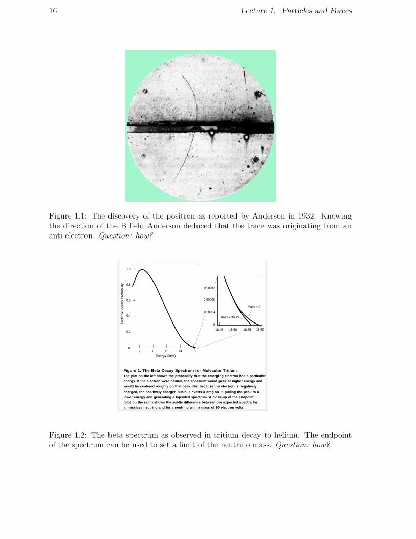
• Dirac had postulated in 1927 the existance of anti-matter as a consequence of hisrelativistic version of the Schrodinger equation in quantum mechanics. (We willcome back to the Dirac theory later on.) The anti-matter partner of the electron,the positron, was actually discovered in 1932 by Anderson (see Fig. 1.1).
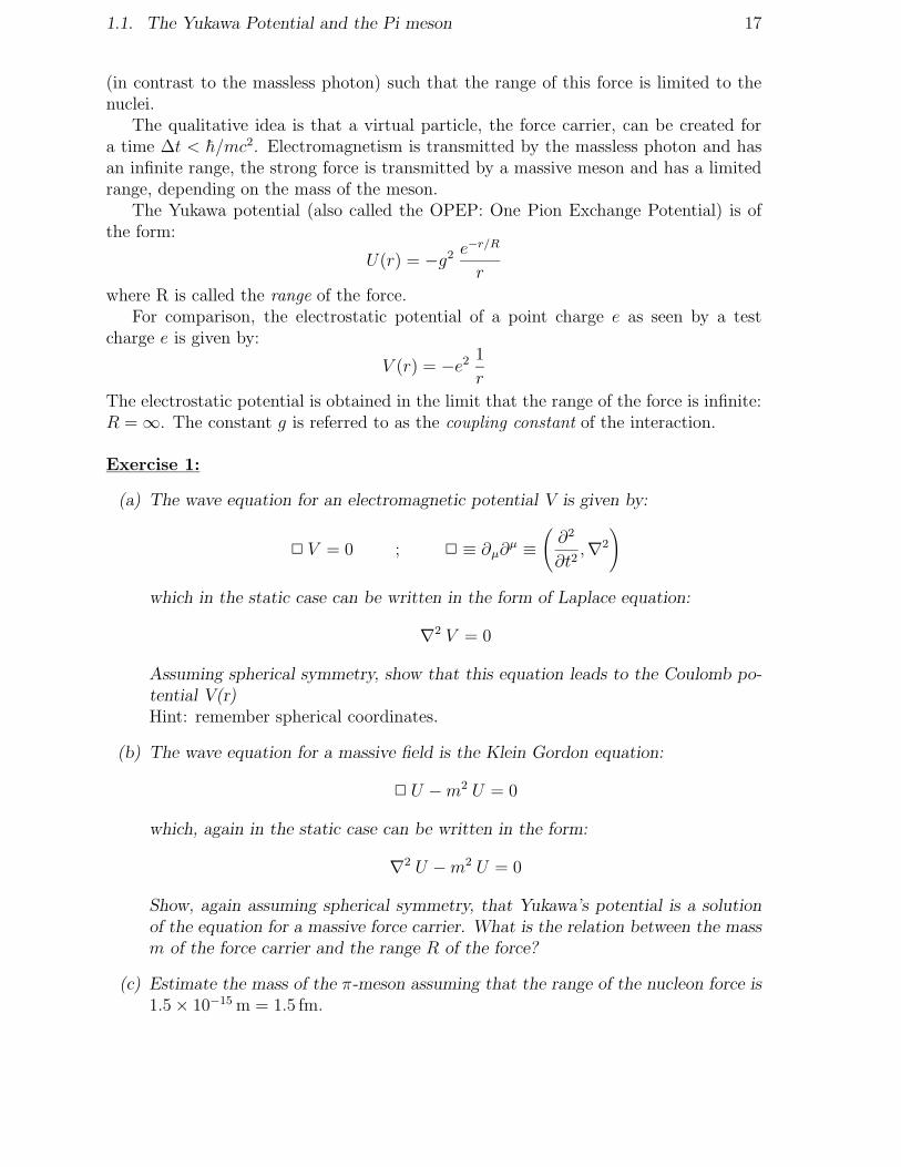
• Pauli had postulated the existance of an invisible particle that was produced innuclear beta decay: the neutrino. In a nuclear beta decay process:
NA → NB + e−
the energy of the emitted electron is determined by the mass difference of the nucleiNA and NB. It was observed that the kinetic energy of the electrons, however,showed a broad mass spectrum (see Fig. 1.2), of which the maximum was equalto the expected kinetic energy. It was as if an additional invisible particle of lowmass is produced in the same process: the (anti-) neutrino.
1.1 The Yukawa Potential and the Pi meson
The year 1935 is a turning point in particle physics. Yukawa studied the strong inter-action in atomic nuclei and proposed a new particle, a π-meson as the carrier of thenuclear force. His idea was that the nuclear force was carried by a massive particle
15
16 Lecture 1. Particles and Forces
Figure 1.1: The discovery of the positron as reported by Anderson in 1932. Knowingthe direction of the B field Anderson deduced that the trace was originating from ananti electron. Question: how?
0.8
0.6
0.4
0.2
1.0
02 6 10 14 18
Energy (keV)
0.00004
0
18.45 18.50 18.55 18.60
0.00012
0.00008
Mass = 0
Mass = 30 eV
Rel
ativ
e D
ecay
Pro
babi
lity
Figure 1. The Beta Decay Spectrum for Molecular Tritium The plot on the left shows the probability that the emerging electron has a particular
energy. If the electron were neutral, the spectrum would peak at higher energy and
would be centered roughly on that peak. But because the electron is negatively
charged, the positively charged nucleus exerts a drag on it, pulling the peak to a
lower energy and generating a lopsided spectrum. A close-up of the endpoint
(plot on the right) shows the subtle difference between the expected spectra for
a massless neutrino and for a neutrino with a mass of 30 electron volts.
Figure 1.2: The beta spectrum as observed in tritium decay to helium. The endpointof the spectrum can be used to set a limit of the neutrino mass. Question: how?
1.1. The Yukawa Potential and the Pi meson 17
(in contrast to the massless photon) such that the range of this force is limited to thenuclei.
The qualitative idea is that a virtual particle, the force carrier, can be created fora time ∆t < h/mc2. Electromagnetism is transmitted by the massless photon and hasan infinite range, the strong force is transmitted by a massive meson and has a limitedrange, depending on the mass of the meson.
The Yukawa potential (also called the OPEP: One Pion Exchange Potential) is ofthe form:
U(r) = −g2 e−r/R
r
where R is called the range of the force.For comparison, the electrostatic potential of a point charge e as seen by a test
charge e is given by:
V (r) = −e2 1r
The electrostatic potential is obtained in the limit that the range of the force is infinite:R =∞. The constant g is referred to as the coupling constant of the interaction.
Exercise 1:
(a) The wave equation for an electromagnetic potential V is given by:
2 V = 0 ; 2 ≡ ∂µ∂µ ≡
(
∂2
∂t2,∇2
)
which in the static case can be written in the form of Laplace equation:
∇2 V = 0
Assuming spherical symmetry, show that this equation leads to the Coulomb po-tential V(r)Hint: remember spherical coordinates.
(b) The wave equation for a massive field is the Klein Gordon equation:
2 U −m2 U = 0
which, again in the static case can be written in the form:
∇2 U −m2 U = 0
Show, again assuming spherical symmetry, that Yukawa’s potential is a solutionof the equation for a massive force carrier. What is the relation between the massm of the force carrier and the range R of the force?
(c) Estimate the mass of the π-meson assuming that the range of the nucleon force is1.5× 10−15m = 1.5 fm.

18 Lecture 1. Particles and Forces
Yukawa called this particle a meson since it is expected to have an intermediate massbetween the electron and the nucleon. In 1937 Anderson and Neddermeyer, as well asStreet and Stevenson, found that cosmic rays indeed consist of such a middle weightparticle. However,in the years after, it became clear that two things were not right:
(1) This particle did not interact strongly, which was very strange for a carrier of thestrong force.
(2) Its mass was somewhat too low.
In fact this particle turned out to be the muon, the heavier brother of the electron.In 1947 Powell (as well as Perkins) found the pion to be present in cosmic rays. They
took their photographic emulsions to mountain tops to study the contents of cosmic rays(see Fig. 1.3). (In a cosmic ray event a cosmic proton scatters with high energy on anatmospheric nucleon and produces many secondary particles.) Pions produced in theatmosphere decay long before they reach sea level, which is why they were not observedbefore.
1.2 Strange Particles
After the pion had been identified as Yukawa’s strong force carrier and the anti-electronwas observed to confirm Dirac’s theory, things seemed reasonably under control. Themuon was a bit of a mystery. It lead to a famous quote of Isidore Rabi at the conference:“Who ordered that?”
But in December 1947 things went all wrong after Rochester and Butler publishedso-called V 0 events in cloud chamber photographs. What happened was that chargedcosmic particles hit a lead target plate and as a result many different types of particleswere produced. They were classified as:
baryons: particles whose decay product ultimately includes a proton.
mesons: particles whose decay product ultimately include only leptons or photons.
Why were these events called strange? The mystery lies in the fact that certain (neutral)particles were produced (the “V 0’s”) with a large cross section ( ∼ 10−27cm2), while theydecay according to a process with a small cross section (∼ 10−40cm2). The explanationto this riddle was given by Abraham Pais in 1952 and is called associated production.This means that strange particles are always produced in pairs by the strong interaction.It was suggested that strange particle carries a strangeness quantum number. In thestrong interaction one then has the conservation rule ∆S = 0, such that a particle withS=+1 (e.g. a K meson) is simultaneously produced with a particle with S=-1 (e.g. aΛ baryon). These particles then individually decay through the weak interaction, whichdoes not conserve strangeness. An example of an associated production event is seen inFig. 1.4.

1.2. Strange Particles 19
Figure 1.3: A pion entering from the left decays into a muon and an invisible neutrino.

20 Lecture 1. Particles and Forces
Figure 1.4: A bubble chamber picture of associated production.

1.3. The Eightfold Way 21
In the years 1950 - 1960 many elementary particles were discovered and one startedto speak of the particle zoo. A quote: “The finder of a new particle used to be awardedthe Nobel prize, but such a discovery now ought to be punished by a $10.000 fine.”
1.3 The Eightfold Way
In the early 60’s Murray Gell-Mann (at the same time also Yuvan Ne’eman) observedpatterns of symmetry in the discovered mesons and baryons. He plotted the spin 1/2baryons in a so-called octet (the “eightfold way” after the eighfold way to Nirvana inBuddhism). There is a similarity between Mendeleev’s periodic table of elements andthe supermultiplets of particles of Gell Mann. Both pointed out a deeper structure ofmatter. The eightfold way of the lightest baryons and mesons is displayed in Fig. 1.5and Fig. 1.6. In these graphs the Strangeness quantum number is plotted vertically.
Q=+1
n
Σ Σ Σ
Ξ
p
Ξ
Λ
+
+0
− 0
−
Q=−1 Q=0
S=0
S=−1
S=−2
Figure 1.5: Octet of lightest baryons with spin=1/2.
S=−1
+−
Q=−1 Q=0 Q=1
K
Π ΠΠη
0
K0
−Κ0Κ−
+S=1
S=0
Figure 1.6: Octet with lightest mesons of spin=0
Also heavier hadrons could be given a place inmultiplets. The baryons with spin=3/2were seen to form a decuplet, see Fig. 1.7. The particle at the bottom (at S=-3) had notbeen observed. Not only was it found later on, but also its predicted mass was found tobe correct! The discovery of the Ω− particle is shown in Fig. 1.8.

22 Lecture 1. Particles and Forces
~1680 MeV
Σ Σ
∆∆ ∆ ∆−∗ ∗+
Σ∗0
− 0 + ++
Ξ Ξ∗ ∗− 0
Ω−
Q=−1
Q=0
Q=+1
Q=+2
S=0
S=−1
S=−2
S=−3
mass
~1230 MeV
~1380 MeV
~1530 MeV
Figure 1.7: Decuplet of baryons with spin=3/2. The Ω− was not yet observed whenthis model was introduced. It’s mass was predicted.
Figure 1.8: Discovery of the omega particle.

1.4. The Quark Model 23
1.4 The Quark Model
The observed structure of hadrons in multiplets hinted at an underlying structure. Gell-Mann and Zweig postulated indeed that hadrons consist of more fundamental partons:the quarks. Initially three quarks and their anti-particle were assumed to exist (see Fig.1.9). A baryon consists of 3 quarks: (q, q, q), while a meson consists of a quark and anantiquark: (q, q). Mesons can be their own anti-particle, baryons cannot.
uS=0
S=−1 Q=+2/3
Q=−1/3
s
d S=+1 s
d
Q=+1/3Q=−2/3
S=0u
Figure 1.9: The fundamental quarks: u,d,s.
Exercise 2:Assign the quark contents of the baryon decuplet and the meson octet.
How does this explain that baryons and mesons appear in the form of octets, decu-plets, nonets etc.? For example a baryon, consisting of 3 quarks with 3 flavours (u,d,s)could in principle lead to 3x3x3=27 combinations. The answer lies in the fact thatthe wave function of fermions is subject to a symmetry under exchange of fermions.The total wave function must be anti-symmetric with respect to the interchange of twofermions.
ψ (baryon) = ψ (space) · φ (spin) · χ (flavour) · ζ (color)These symmetry aspects are reflected in group theory where one encounters expressionsas: 3⊗ 3⊗ 3 = 10⊕ 8⊕ 8⊕ 1 and 3⊗ 3 = 8⊕ 1.
For more information on the static quark model read chapter 5 in the book of Perkinsor chapter 10 in the book of Burcham & Jobes.
1.4.1 Color
As indicated in the wave function above, a quark has another internal degree of freedom.In addition to electric charge a quark has a different charge, of which there are 3 types.This charge is referred to as the color quantum number, labelled as r, g, b. Evidencefor the existence of color comes from the ratio of the cross section:
R ≡ σ(e+e− → hadrons)
σ(e+e− → µ+µ−)= NC
∑
i
Q2i
where the sum runs over the quark types that can be produced at the available energy.The plot in Fig. 1.10 shows this ratio, from which the result NC = 3 is obtained.

24 Lecture 1. Particles and Forces
10-1
1
10
10 2
10 3
1 10 102
R ω
ρ
φ
ρ′
J/ψ ψ(2S)
Υ
Z
√
s [GeV]Figure 1.10: The R ratio.
Exercise 3: The Quark Model
(a) Quarks are fermions with spin 1/2. Show that the spin of a meson (2 quarks) canbe either a triplet of spin 1 or a singlet of spin 0.Hint: Remember the Clebsch Gordon coefficients in adding quantum numbers.In group theory this is often represented as the product of two doublets leads tothe sum of a triplet and a singlet: 2⊗ 2 = 3⊕ 1 or, in terms of quantum numbers:1/2⊗ 1/2 = 1⊕ 0.
(b) Show that for baryon spin states we can write: 1/2⊗ 1/2⊗ 1/2 = 3/2⊕ 1/2⊕ 1/2or equivalently 2⊗ 2⊗ 2 = 4⊕ 2⊕ 2
(c) Let us restrict ourselves to two quark flavours: u and d. We introduce a newquantum number, called isospin in complete analogy with spin, and we refer tothe u quark as the isospin +1/2 component and the d quark to the isospin -1/2component (or u= isospin “up” and d=isospin “down”). What are the possibleisospin values for the resulting baryon?
(d) The ∆++ particle is in the lowest angular momentum state (L = 0) and hasspin J3 = 3/2 and isospin I3 = 3/2. The overall wavefunction (L⇒space-part,S⇒spin-part, I⇒isospin-part) must be anti-symmetric under exchange of any ofthe quarks. The symmetry of the space, spin and isospin part has a consequencefor the required symmetry of the Color part of the wave function. Write downthe color part of the wave-function taking into account that the particle is colorneutral.
(e) In the case that we include the s quark the flavour part of the wave functionbecomes: 3⊗ 3⊗ 3 = 10⊕ 8⊕ 8⊕ 1.In the case that we include all 6 quarks it becomes: 6⊗ 6⊗ 6. However, this isnot a good symmetry. Why not?

1.5. The Standard Model 25
1.5 The Standard Model
The fundamental constituents of matter and the force carriers in the Standard Modelcan be represented as follows:
The fundamental particles:charge Quarks
23
u (up) c (charm) t (top)1.5–4MeV 1.15–1.35GeV (174.3± 5.1)GeV
−13
d (down) s (strange) b (bottom)4–8MeV 80–130MeV 4.1–4.4GeV
charge Leptons
0 νe (e neutrino) νµ (µ neutrino) ντ (τ neutrino)< 3 eV < 0.19MeV < 18.2MeV
−1 e (electron) µ (muon) τ (tau)0.511MeV 106MeV 1.78GeV
The forces, their mediating bosons and their relative strength:Force Boson Relative strengthStrong g (8 gluons) αs ∼ O(1)
Electromagnetic γ (photon) α ∼ O(10−2)Weak Z0,W± (weak bosons) αW ∼ O(10−6)
Some definitions:
hadron (greak: strong) particle that feels the strong interactionlepton (greak: light, weak) particle that feels only weak interactionbaryon (greak: heavy) particle consisting of three quarksmeson (greak: middle) particle consisting of a quark and an anti-quarkpentaquark a hypothetical particle consisting of 4 quarks and an anti-quarkfermion half-integer spin particleboson integer spin particlegauge-boson force carrier as predicted from local gauge invariance
In the Standard Model forces originate from a mechanism called local gauge invari-ance, which wil be discussed later on in the course. The strong force (or color force) ismediated by gluons, the weak force by intermediate vector bosons, and the electromag-netic force by photons. The fundamental diagrams are represented below.
There is an important difference between the electromagnetic force on one hand, andthe weak and strong force on the other hand. The photon does not carry charge and,

26 Lecture 1. Particles and Forces
a:γ
e+
e−
µ+
µ−
b: W
e−
νe
νµ
µ−
c:g
q
q
q
q
Figure 1.11: Feynman diagrams of fundamental lowest order perturbation theory pro-cesses in a: electromagnetic, b: weak and c: strong interaction.
therefore, does not interact with itself. The gluons, however, carry color and do interactamongst each other. Also, the weak vector bosons carry weak isospin and undergo aself coupling.
The strength of an interaction is determined by the coupling constant as well as themass of the vector boson. Contrary to its name the couplings are not constant, butvary as a function of energy. At a momentum transfer of 1015 GeV the couplings ofelectromagnetic, weak and strong interaction all have the same value. In the quest ofunification it is often assumed that the three forces unify to a grand unification force atthis energy.
Due to the self coupling of the force carriers the running of the coupling constantsof the weak and strong interaction are opposite to that of electromagnetism. Electro-magnetism becomes weaker at low momentum (i.e. at large distance), the weak and thestrong force become stronger at low momentum or large distance. The strong interac-tion coupling even diverges at momenta less than a few 100 MeV (the perturbative QCDdescription breaks down). This leads to confinement: the existence of colored objects(i.e. objects with net strong charge) is forbidden.
Finally, the Standard Model includes a, not yet observed, scalar Higgs boson, whichprovides mass to the vector bosons and fermions in the Brout-Englert-Higgs mechanism.

1.5. The Standard Model 27
Figure 1.12: Running of the coupling constants and possible unification point.
Open Questions
• Does the Higgs in fact exist?
• Why are the masses of the particles what they are?
• Why are there 3 generations of fermions?
• Are quarks and leptons truly fundamental?
• Why is the charge of the electron exactly opposite to that of the proton. Or: whyis the total charge of leptons and quarks exactly equal to 0?
• Is a neutrino its own anti-particle?
• Can all forces be described in a single theory (unification)?
• Why is there no anti matter in the universe?
• What is the source of dark matter?
• What is the source of dark energy?

28 Lecture 1. Particles and Forces

Lecture 2
Wave Equations and Anti Particles
Introduction
In the course we develop a quantum mechanical framework to describe electromagneticscattering, in short Quantum Electrodynamics (QED). The way we build it up is thatwe first derive a framework for non-relativistic scattering of spinless particles, whichwe then extend to the relativistic case. Also we will start with the wave equations forparticles without spin, and address the spin 1/2 particles later on in the lectures (“theDirac equation’).
What is a spinless particle? There are two ways that you can think of it: either ascharged mesons (e.g. pions or kaons) for which the strong interaction has been “switchedoff” or for electrons or muons for which the fact that they are spin-1/2 particles isignored. In short: it not a very realistic case.
2.1 Non Relativistic Wave Equations
If we start with the non relativistic relation between kinetic energy and momentum
E =~p2
2m
and make the quantum mechanical substitution:
E → i∂
∂tand ~p→ −i~∇
then we end up with Schrodinger’s equation:
i∂
∂tψ =
−12m
∇2ψ
In electrodynamics we have the continuity equation (“Gauss law”) which relates acurrent to a change of charge:
~∇ ·~j = −∂ρ∂t
29

30 Lecture 2. Wave Equations and Anti Particles
where j = the current density and ρ = the charge density.This is a rather general law stat can be stated in words as: “The change of charge
in a given volume equals the current through the surrounding surface.”Can we make use of the continuity equation in quantum mechnics? Let us mul-
tiply the Schrodinger equation from the left by ψ∗ and do the same for the complexconjugates:
ψ∗ i∂ψ
∂t= ψ∗
(−12m
)
∇2ψ
ψ − i∂ψ∗
∂t= ψ
(−12m
)
∇2ψ∗
−∂
∂t(ψ∗ ψ)︸ ︷︷ ︸
ρ
= −~∇ ·[i
2m
(
ψ ~∇ψ∗ − ψ∗ ~∇ψ)]
︸ ︷︷ ︸
~j
In the result we can recognize again the continuity equation if we interpret the densityand current as indicated.
Example: Consider a solution to the Schrodinger equation for a free particle:
ψ = N ei(~p~x−Et) ( show it is a solution )
then:
ρ = ψ∗ ψ = |N |2
~j =i
2m
(
ψ ~∇ψ∗ − ψ∗ ~∇ψ)
=|N |2m
~p
Exercise 4:Derive the expressions for ρ and ~j explicitly.
2.2 Relativistic Wave Equations
If we start with the relativistic equation:
E2 = p2 +m2
and again make the substitution:
E → i∂
∂tand ~p→ −i~∇
then we end up with the Klein Gordon equation for a wavefunction φ:
− ∂2
∂t2φ = −∇2φ+m2 φ

2.2. Relativistic Wave Equations 31
or in 4-vector notation:(
2 +m2)
φ(x) = 0
or :(
∂µ∂µ +m2
)
φ(x) = 0
A solution is again provided by plane waves:
φ(x) = N e−ipµxµ
with eigenvalues E2 = ~p2 +m2
In the same way as before we can define a current density by multiplying the K.G.equation for φ from the left with φ∗ and doing the same to the complex conjugateequation:
−iφ∗(
−∂2φ
∂t2
)
= −iφ∗(
−∇2φ+m2 φ)
iφ
(
−∂2φ∗
∂t2
)
= iφ(
−∇2φ∗ +m2φ∗)
+∂
∂ti
(
φ∗∂φ
∂t− φ
∂φ
∂t
)
︸ ︷︷ ︸
ρ
= ~∇ ·[
i(
φ∗ ~∇φ− φ ~∇φ∗)]
︸ ︷︷ ︸
~j
where we can recognize again the continuity equation. In 4-vector notation it becomes:
jµ =(
ρ,~j)
= i [φ∗ (∂µφ)− (∂µφ∗)φ]
∂µjµ = 0
Let us substitute the plane wave solutions φ = N e−ipx then:
ρ = 2 |N |2 E~j = 2 |N |2 ~p
or : → jµ = 2 |N |2 pµ
Exercise 5:Derive the expressions for ρ and ~j explicitly.
But now we really have an interpretation problem! There are two solutions: E = ±√~p2 +m2.
The solution with E < 0 is difficult to interpret as it means ρ < 0.
Exercise 6:The relativitic energy-momentum relation can be written as:
E =√
p2 +m2 (2.1)
This is linear in E = ∂/∂t, but we don’t know what to do with the square root of themomentum operator. However, for small p we can expand the expression in powers ofp. Do this up and including to order p2 and write down the resulting wave equation.Determine the probability density and the current density.

32 Lecture 2. Wave Equations and Anti Particles
−m
E
+m
E
+m
−m
Figure 2.1: Dirac’s interpretation of negative energy solutions: “holes”
2.3 Interpretation of negative energy solutions
2.3.1 Dirac’s interpretation
In 1927 Dirac offered a new interpretation of the negative energy states. He introduceda new wave equation which in fact was linear in time and space, which will be discussedlater on in the course. It turned out to automatically describe particles with spin 1/2.At this point in the course we consider spinless particles. Stated otherwise: the wavefunction ψ or φ is a scalar quantity as there is no individual spin “up” or spin “down”component.
According to the Pauli exclusion principle, Dirac knew that there can not be twoidentical particles in the same quantum state. Dirac’s picture of the vacuum and of aparticle are schematically represented in Fig. 2.1.
The plot shows all the avaliable energy levels of an electron. It’s lowest absoluteenergy level is given by |E| = m. Dirac imagined the vacuum to contain an infinitenumber of states with negative energy which are all occupied. Since an electron isa spin-1/2 particle each state can only contain one spin “up” electron and one spin-”down” electron. All the negative energy levels are filled. Such a vacuum (“sea”) is notdetectable since the electrons in it cannot interact, i.e. go to another state.
If energy is added to the system, an electron can be kicked out of the sea. It nowgets a positive energy with E > m. This means this electron becomes visible as it cannow interact. At the same time a “hole” in the sea has appeared. This whole can beinterpreted as a positive charge at that position. Dirac’s hope was that he could describethe proton in such a way.

2.3. Interpretation of negative energy solutions 33
2.3.2 Pauli-Weisskopf Interpretation
Pauli and Weiskopf proposed a simpler scheme in 1934 in which they re-interpreted theopposite sign solutions of the Klein Gordon equation as the opposite charges:ρ = electric charge density~j = electric current densityand the − and + solutions indicate the electron and positron. The positron then hadof course the mass as the electron. The positron was discovered in 1934 by Anderson.
2.3.3 Feynman-Stuckelberg Interpretation
The current density for a particle with charge −e and momentum (E, ~p) is:
jµ(−e) = −2e |N |2 pµ = −2e |N |2 (E, ~p)
The current density for a particle with charge +e and momentum (E, ~p) is:
jµ(+e) = +2e |N |2 pµ = −2e |N |2 (−E,−~p)
This means that the positive energy solution for a positron is the negative energysolution for an electron.
Note that indeed the wave function Neipx = Neipµxµ
is invariant under: pµ → −pµand xµ → −xµ. So the wave functions which describe particles also describe anti-particles. The negative energy solutions give particles travelling backwards in time.They are the same as the positive energy solutions of anti-particles travelling forwardin time. This is indicated in Fig. 2.2.
e e
E>0 E<0
+ −
t
Figure 2.2: A positron travelling forward in time is an electron travelling backwards intime.
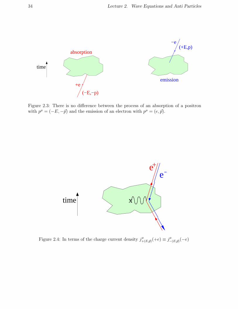
As a consequence of the Feynman-Stuckelberg interpretation the process of an ab-sorption of a positron with energy −E is the same as the emission of an electron withenergy E (see Fig.2.3). In the calculations with Feynman diagrams we have made theconvention that all scattering processes are calculated in terms of particles and not an-tiparticles. As an example, the process of an incoming positron scattering off a potentialwill be calculated as that of an electron travelling back in time (see Fig. 2.4).
Let us consider the scattering of an electron in a potential. The probability of aprocess is calculated in perturbation theory in terms of basic scattering processes (i.e.
34 Lecture 2. Wave Equations and Anti Particles
(+E,p)
emission
absorption
−e
+e
time
(−E,−p)
Figure 2.3: There is no difference between the process of an absorption of a positronwith pµ = (−E,−~p) and the emission of an electron with pµ = (e, ~p).
+
time x
ee−
Figure 2.4: In terms of the charge current density jµ+(E,~p)(+e) ≡ jµ−(E,~p)(−e)

2.3. Interpretation of negative energy solutions 35
Feynman diagrams). In Fig. 2.5 the first and second order scattering of the electron isillustrated. To first order a single photon carries the interaction between the electron andthe potential. When the calculation is extended to second order the electron interactstwice with the field. It is interesting to note that this scattering can occur in twotime orderings as indicated in the figure. Note that the observable path of the electronbefore and after the scattering process is identical in the two processes. Because of ouranti-particle interpretation, the second picture is also possible. It can be viewed in twoways:
• The electron scatters at time t2 runs back in time and scatters at t1.
• First at time t1 “spontaneously” an e−e+ pair is created from the vacuum. Later-on, at time t2, the produced positron annihilates with the incoming electron, whilethe produced electron emerges from the scattering process.
In quantum mechanics both time ordered processes (the left and the right picture)must be included in the calculation of the cross section. We realize that the vacuumhas become a complex environment since particle pairs can spontaneously emerge fromit and dissolve into it!
2
x
e−time
e−
x
x
e− e−
−e
x
xtt12
tt1
Figure 2.5: First and second order scattering.
36 Lecture 2. Wave Equations and Anti Particles
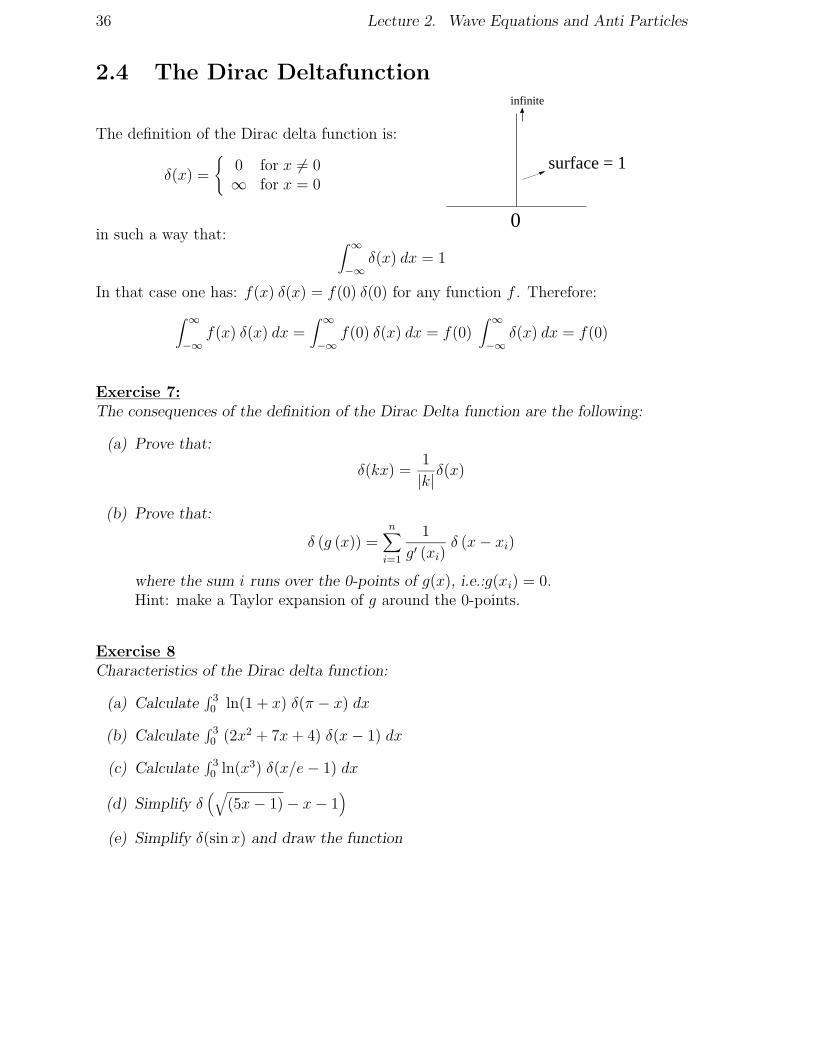
2.4 The Dirac Deltafunction
The definition of the Dirac delta function is:
δ(x) =
0 for x 6= 0∞ for x = 0
0
surface = 1
infinite
in such a way that:∫ ∞
−∞δ(x) dx = 1
In that case one has: f(x) δ(x) = f(0) δ(0) for any function f . Therefore:
∫ ∞
−∞f(x) δ(x) dx =
∫ ∞
−∞f(0) δ(x) dx = f(0)
∫ ∞
−∞δ(x) dx = f(0)
Exercise 7:The consequences of the definition of the Dirac Delta function are the following:
(a) Prove that:
δ(kx) =1
|k|δ(x)
(b) Prove that:
δ (g (x)) =n∑
i=1
1
g′ (xi)δ (x− xi)
where the sum i runs over the 0-points of g(x), i.e.:g(xi) = 0.Hint: make a Taylor expansion of g around the 0-points.
Exercise 8Characteristics of the Dirac delta function:
(a) Calculate∫ 30 ln(1 + x) δ(π − x) dx
(b) Calculate∫ 30 (2x2 + 7x+ 4) δ(x− 1) dx
(c) Calculate∫ 30 ln(x3) δ(x/e− 1) dx
(d) Simplify δ(√
(5x− 1)− x− 1)
(e) Simplify δ(sinx) and draw the function

Lecture 3
The Electromagnetic Field
3.1 Maxwell Equations
As we eventually want to calculate processes in QED, let us look at the electromagneticfield and the photon. The Maxwell equations in vacuum are:
(1) ~∇ · ~E = ρ Gauss law
(2) ~∇ · ~B = 0 No magnetic poles
(3) ~∇× ~E +∂ ~B
∂t= 0 Faraday′s law of induction
(4) ~∇× ~B − ∂ ~E
∂t= ~j Relate B field to a current
From the first and the fourth equation we can indeed derive the continuity equation:
~∇ ·~j = −∂ρ∂t
In scattering with particles we want to work relativistic, so it would be suitable ifwe could formulate Maxwell equartions in a covariant way; i.e. in a manifestly Lorentzinvariant way.
To do this we introduce a mathematical tool: the potential Aµ =(
V, ~A)
. We note
at this point that the fields ~E, ~B are physical, while the potential is not. Rememberthat the following identities are valid for any vector field ~A and scalar field V :
~∇×(
~∇V)
= 0 ( rotation of gradient is 0 )
~∇ ·(
~∇× ~A)
= 0 ( divergence of a rotation is 0 )
We choose the potential in such a way that two Maxwell equations are automaticallyfullfilled:
1. ~B = ~∇× ~AThen, automatically it follows that: ~∇ · ~B = 0.
37
38 Lecture 3. The Electromagnetic Field
2. ~E = −∂ ~A∂t− ~∇V
Then, automatically it follows that: ~∇× ~E = −∂(~∇× ~A)∂t
− 0 = −∂ ~B∂t.
So, by a suitable defition of how the potential Aµ is related to the physical fields,automatically Maxwell equations (2) and (3) are fullfilled.
Exercise 9:Derive the expressions for ρ and ~j explicitly.
(a) Show that Maxwell’s equations can be written as:
∂µ∂µAν − ∂ν∂µA
µ = jν
Hint: Note that ~∇×(
~∇× ~A)
= −∇2 ~A+ ~∇(
~∇ · ~A)
(b) It can be made even more compact by introducing the tensor: F µν ≡ ∂µAν−∂νAµ.Show that with this definition Maxwell’s equations reduce to:
∂µFµν = jν
Intermezzo: 4-vector notation
Assume that we have a contravariant vector:
Aµ =(
A0, A1, A2, A3)
=(
A0, ~A)
then the covariant vector is obtained as:
Aν = (A0, A1, A2, A3) = gµνAµ =
(
A0,−A1,−A2 − A3)
=(
A0,− ~A)
since we use the metric sensor:
gµν = gµν =
1 0 0 00 −1 0 00 0 −1 00 0 0 −1
There is one exception to this: ∂µ ≡ ∂∂xµ
. For the derivative 4-vector we then find:
∂µ =
(
∂
∂t, ~∇)
∂µ =
(
∂
∂t,−~∇
)
which is opposite to the contravariant and covariant behaviour of a usual 4-vector Aµ
defined above.
3.2. Gauge Invariance 39
3.2 Gauge Invariance
Since we have introduced the potential Aµ as a mathematical tool rather than as aphysical field we can choose any Aµ potential as long as the ~E and ~B fields don’t change.After re-examining the equations that define A we realize that there is a freedom to makeso-caled gauge transformations which do not affect the physical fields ~E and ~B:
Aµ → Aµ′ = Aµ + ∂µλ or
Aµ → Aµ′ = Aµ + ∂µλ for any λ
In terms of the Voltage V and vectors potential ~A we have:
V ′ = V +∂λ
∂t~A′ = ~A− ~∇λ
Exercise 10:Show explicitly that in such gauge transformations the ~E and ~B fields do not change:
~B′ = ~∇× ~A′ = ... = ~B
~E ′ = −∂~A′
∂t− ~∇V ′ = ... = ~E
The laws of physics are gauge invariant. This implies that we can choose any gaugeto calculate physics quantities. It is most elegant if we can perform all calculations ina way that is manifestly gauge invariant. However, sometimes we choose a particulargauge in order to make the expressions in calculations simpler.
A gauge choice that is often made is called the Lorentz condition, in which we chooseAµ according to:
∂µAµ = 0
Exercise 11:Show that it is always possible to define a Aµ field according to the Lorentz gauge. Todo this assume that for a given Aµ field one has: ∂µA
µ 6= 0. Give then the equation forthe gauge field λ by which the A field must be transformed to obtain the Lorentz gauge.
In the Lorentz gauge the Maxwell equations simplify further:
∂µ∂µAν − ∂ν∂µA
µ = jν now becomes :
∂µ∂µAν = jν
40 Lecture 3. The Electromagnetic Field
However, Aµ still has some freedom since we have fixed: ∂µ (∂µλ), but we have not
yet fixed ∂µλ! In other words a gauge transformation of the form:
Aµ → A′µ = Aµ + ∂µλ with : 2λ = ∂µ∂µλ = 0
is still allowed within the Lorentz gauge ∂µAµ = 0. However, we can in addition impose
the Coulomb condition:
A0 = 0 or equivalently : ~∇ · ~A = 0
At the same time we realize, however, that this is not elegant as we give the “0-th component” or “time-component” of the 4-vector a special treatment. Therefore thechoice of this gauge is not Lorentz invariant. This means that one has to chose a differentgauge condition if one goes from one reference frame to a different reference frame. Thisis allowed since the choice of the gauge is irrelevant for the physics observables, but itsometimes considered “not elegant”.
3.3 The photon
Let us turn to the wave function of the photon. We start with Maxwell’s equation andconsider the case in vacuum:
2Aµ = jµ → vacuum : jµ = 0 → 2Aµ = 0
Immediately we recognize that this is the Klein Gordon equation of a quantum mechan-ical particle with mass m = 0: (2 +m2)φ(x) = 0 (see previous Lecture). This particleis the photon.
The plane wave solutions of the massless K.-G. equation are:
Aµ (x) = Nεµ (p) e−ipx with : p2 = pµpµ = 0
We are describing vector field Aµ since the field has a Lorentz index µ. The vectorεµ(p) is the polarization vector: it has 4 degrees of freedom. Does this mean that thephoton has 4 polarizations?
Let us take a look at the gauge conditions and we see that there are some restrictions:
• Lorentz condition:
∂µAµ = 0 ⇒ pµ ε
µ = 0
This reduces the number of independent components to three. For the gauge fieldthis implies 2λ = 0 and we see that we can choose the gauge field as:
λ = iae−ipx
∂µλ = apµe−ipx
3.3. The photon 41
where a is a constant. Thus the gauge transformation looks like
Aµ → A′µ = N(
εµe−ipx + apµe
−ipx)
or, in terms of the polarization vector:
εµ → ε′µ = εµ + apµ
Therefore, different polarization vectors which differ by a multiple of pµ describethe same physical photon.
• Coulomb condition:
We choose the zero-th component of the gauge field such that: ε0 = 0. Then theLorentz condition reduces to:
A0 = 0~∇ · ~A = 0
⇒
ε0 = 0~ε · ~p = 0
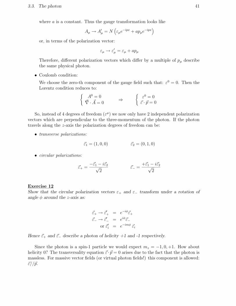
So, instead of 4 degrees of freedom (εµ) we now only have 2 independent polarizationvectors which are perpendicular to the three-momentum of the photon. If the photontravels along the z-axis the polarization degrees of freedom can be:
• transverse polarizations:
~ε1 = (1, 0, 0) ~ε2 = (0, 1, 0)
• circular polarizations:
~ε+ =−~ε1 − i~ε2√
2~ε− =
+~ε1 − i~ε2√2
Exercise 12Show that the circular polarization vectors ε+ and ε− transform under a rotation ofangle φ around the z-axis as:
~ε+ → ~ε′+ = e−iφ~ε+
~ε− → ~ε′− = eiφ~ε−
or ~ε′i = e−imφ ~εi
Hence ~ε+ and ~ε− describe a photon of helicity +1 and -1 respectively.
Since the photon is a spin-1 particle we would expect mz = −1, 0,+1. How abouthelicity 0? The transversality equation ~ε · ~p = 0 arises due to the fact that the photon ismassless. For massive vector fields (or virtual photon fields!) this component is allowed:~ε//~p.
42 Lecture 3. The Electromagnetic Field
3.4 The Bohm Aharanov Effect
Later on in the course we will see that the presence of a vector field ~A affects the phaseof a wave function of the particle. The phase factor is affected by the presence of thefield in the following way:
ψ′ = eiqhα(~r,t)ψ
where q is the charge of the particle, h is Plancks constant, and α is given by:
α(~r, t) =∫
rd~r′ · A(~r′, t)
Let us now go back to the famous two-slit experiment of Feynman in which heconsiders the interference between two possible electron trajectories. From quantummechanics we know that the intensity at a detection plate positioned behind the twoslits shows an interference pattern depending on the relative phases of the wave functionsψ1 and ψ2 that travel different paths. For a beautiful description of this effect see chapter1 of the “Feynman Lectures on Physics” volume 3. The idea is schematically depictedin Fig. 3.1.
2
slits
detector
Intensity
coilsource ψ
1
ψ
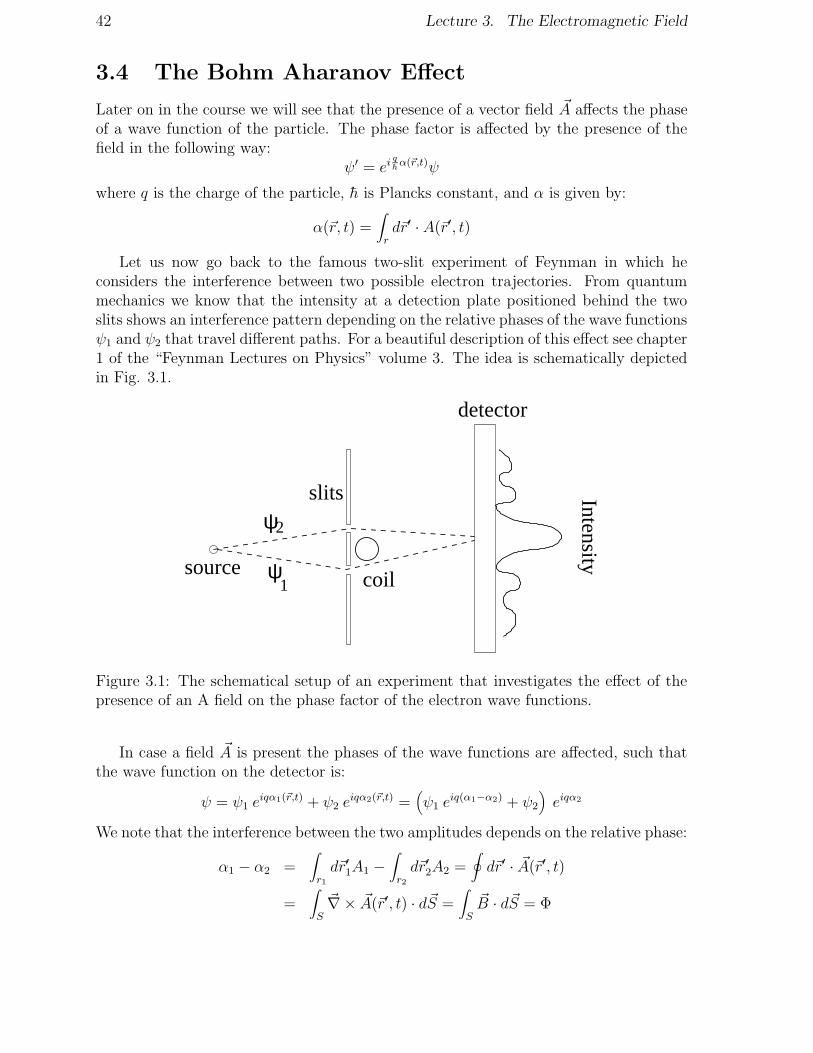
Figure 3.1: The schematical setup of an experiment that investigates the effect of thepresence of an A field on the phase factor of the electron wave functions.
In case a field ~A is present the phases of the wave functions are affected, such thatthe wave function on the detector is:
ψ = ψ1 eiqα1(~r,t) + ψ2 e
iqα2(~r,t) =(
ψ1 eiq(α1−α2) + ψ2
)
eiqα2
We note that the interference between the two amplitudes depends on the relative phase:
α1 − α2 =∫
r1d~r′1A1 −
∫
r2d~r′2A2 =
∮
d~r′ · ~A(~r′, t)
=∫
S
~∇× ~A(~r′, t) · d~S =∫
S
~B · d~S = Φ

3.4. The Bohm Aharanov Effect 43
where we have used Stokes theorem to relate the integral around a closed loop to themagnetic flux through the surface. In this way the presence of a magnetic field canaffect, (i.e. shift) the interference pattern on the screen.
Let us now consider the case that a very long and thin solenoid is positioned in thesetup of the two-slit experiment. Inside the solenoid the B-field is homogeneous andoutside it is B = 0 (or sufficiently small), see Fig. 3.2. However, from electrodynamics
we recall the ~A field is not zero outside the coil. There is a lot of ~A circulation aroundthe thin coil. The electrons in the experiment pass through this ~A field which quantummechanically affects the phase of their wave function and therefor also the interferencepattern on the detector. On the other hand, there is no B field in the region, soclassically there is no effect. Experimentally it has been verified (in a technically difficultexperiment) that the interference pattern will indeed shift.
A
B
Figure 3.2: Magnetic field and vector potential of a long solenoid.
Discussion:
We have introduced the vector potential as a mathematical tool to write Maxwellsequations in a Lorentz covariant form. In this formulation we noticed that the A-fieldhas some arbitraryness due to gauge invariance. Quantummechanically we observe,however, that the A field is not just a mathematical tool, but gives a more fundamentaldescription of “forces”. The aspect of gauge invariance seems an unwanted (“not nice”)aspect now, but later on it will turn out to be a fundamental concept in our descriptionof interactions.
44 Lecture 3. The Electromagnetic Field
Exercise 13The delta function
(a) Show thatd3p
(2π)32E(3.1)
is Lorentz invariant (d3p = dpxdpydpz). Do this by showing that
∫
M(~p)d3p
E=∫
M(p) 2d4p δ(p2 −m2). (3.2)
The 4-vector p is (E, px, py, pz), and M(p) is a Lorentzinvariant function of p.
(b) The delta-function can have many forms. One of them is:
δ(x) = limα→∞
1
π
sin2 αx
αx2(3.3)
Make this plausible by sketching the function sin2(αx)/(παx2) for two relevantvalues of α.
Lecture 4
Perturbation Theory and Fermi’sGolden Rule
4.1 Non Relativistic Perturbation Theory
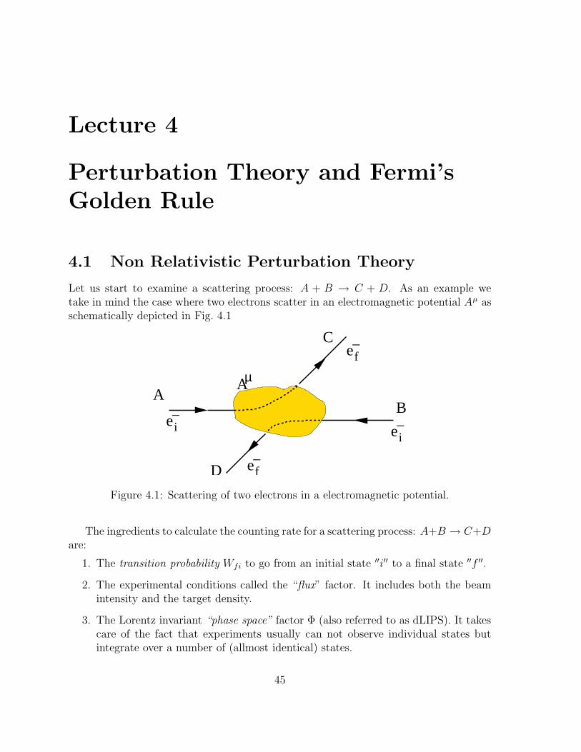
Let us start to examine a scattering process: A + B → C + D. As an example wetake in mind the case where two electrons scatter in an electromagnetic potential Aµ asschematically depicted in Fig. 4.1
µ
B
e
C
e− −
e
e
−
−
A
D
ii
f
f
A
Figure 4.1: Scattering of two electrons in a electromagnetic potential.
The ingredients to calculate the counting rate for a scattering process: A+B → C+Dare:
1. The transition probability Wfi to go from an initial state ′′i′′ to a final state ′′f ′′.
2. The experimental conditions called the “flux” factor. It includes both the beamintensity and the target density.
3. The Lorentz invariant “phase space” factor Φ (also referred to as dLIPS). It takescare of the fact that experiments usually can not observe individual states butintegrate over a number of (allmost identical) states.
45

46 Lecture 4. Perturbation Theory and Fermi’s Golden Rule
The formula for the calculation of a (differential) cross section is:
dσ =Wfi
FluxΦ
Note that the “real” physics, (i.e. the Feynman diagrams) is included in the transitionprobability Wfi. The flux and the phase space factors are the necessary “bookkeeping”needed to compare the physics theory with a realistic experiment. (The calculation ofthe phase space can in fact be rather involved.)
4.1.1 The Transition Probability
In order to calculate the transition probability we use the framework of non-relativisticperturbation theory. In the end we will see how we can use the result in a Lorentzcovariant way and apply it to relativistic scattering.
Consider the scattering of a particle in a potential as depicted in Fig. 4.2 Assumethat before the interaction takes place, as well as after, the system is described by thenon-relativistic Schrodinger equation:
i∂ψ
∂t= H0 ψ
where H0 is the undisturbed Hamiltonian, which does not have a time dependence.Solutions of this equation can be written in the as:
ψm = φm(~x) e−iEmt
with eigenvalues Em.The φm form a complete set orthogonal eigenfunctions of: H0φm = Emφm, so:
∫
φ∗m(~x) φn(~x) d3x = δmn
t=0
H
V(x,t)ψi
ψf
0
0Ht=T/2t=−T/2
Figure 4.2: Scattering of a particle in a potential.

4.1. Non Relativistic Perturbation Theory 47
Assume that at t = 0 a perturbation occurs such that the system is described by:
i∂ψ
∂t= (H0 + V (~x, t)) ψ (4.1)
The solutions ψ can generally be written as:
ψ =∞∑
n=0
an(t) φn(~x) e−iEnt (4.2)
where an(t) is the coefficient to find the system in state “n”.To determine these coefficients an(t) substitute 4.2 in 4.1:
i∞∑
n=0
dan(t)
dtφn(~x) e
−iEnt + i∞∑
n=0
(−i) En an(t) φn(~x) e−iEnt =
∞∑
n=0
En an(t) φn(~x) e−iEnt +
∞∑
n=0
V (~x, t) an(t) φn(~x) e−iEnt
and the two terms proportional to En cancel.Multiply the resulting equation from the left with: ψ∗f = φ∗f (~x) e
iEf t and integrateover volume d3x to obtain:
i∞∑
n=0
dan(t)
dt
∫
d3x φ∗f (~x) φn(~x)︸ ︷︷ ︸
δfn
e−i(En−Ef)t =
∞∑
n=0
an(t)∫
d3x φ∗f (~x) V (~x, t) φn(~x) e−i(En−Ef)t
Next we use the orthonormality relation:
∫
d3x φ∗m(~x) φn(~x) = δmn
so that we find:
daf (t)
dt= −i
∞∑
n=0
an(t)∫
d3x φ∗f (x) V (~x, t) φn(~x) e−i(En−Ef)t
We will assume two simplifications:
• We prepare the incoming wave in a single state: The incoming wave is: ψi =φi(~x) e
−iEit. In other words: ai(−∞) = 1 and an(−∞) = 0 for (n 6= i).
• We will assume that the inital condition is true during the time that the pertur-bation happens! This implies that we work with a weak interaction. In fact this is
the lowest order in perturbation theory in which we replace∞∑
n=0
by just one term:
n = i. It means that af (t) << 1 is assumed at all times.

48 Lecture 4. Perturbation Theory and Fermi’s Golden Rule
The we get:
daf (t)
dt= −i
∫
d3x φ∗f (~x) V (~x, t) φi(~x) e−i(Ei−Ef)t
Our aim is to determine af (t):
af (t′) =
∫ t′
−T/2
daf (t)
dtdt = −i
∫ t′
−T/2dt∫
d3x[
φf (~x) e−iEf t
]∗V (~x, t)
[
φi(~x) e−iEit
]
We define the transition amplitude Tfi as the amplitude to go from state i final state fat the end of the interaction:
Tfi ≡ af (T/2) = −i∫ T/2
−T/2dt∫
d3x φ∗f (~x, t) V (~x, t) φi(~x, t)
Finally we take the limit: T → ∞. Then we can write the expression in 4-vectornotation:
Tfi = −i∫
d4x φ∗f (x) V (x) φi(x)
Note:The expression for Tfi has a manifest Lorentzinvariant form. It is true for each Lorentzframe. Although we started with Schrodinger’s equation (i.e. non-relativistic) we willalways use it: also for relativistic frames.
1-st and 2-nd order perturbation
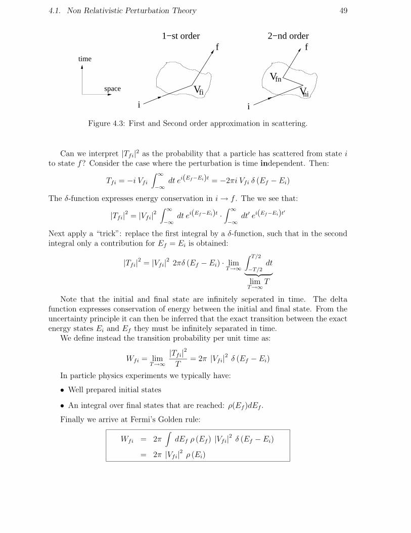
What is the meaning of the initial conditions: ai(t) = 1, an(t) = 0 ? It implies that thepotential can only make one quantum perturbation from the initial state i to the finalstate f . For example the perturbation: i→ n→ f is not included in this approximation(it is a 2nd order perturbation).
If we want to improve the calculation to second order in perturbation theory wereplace the approximation an(t) = 0 by the first order result:
daf (t)
dt= −i Vfi e−i(Ef−Ei)t
+ (−i)2
∑
n6=iVni
∫ t
−T/2dt′ e−i(En−Ei)t
′
Vfn e−i(Ef−En)t
where we have assumed that the perturbation is time independent and introduced thenotation:
Vfi ≡∫
d3xφ∗f (~x) V (~x) φi(~x)
See the book of Halzen and Martin how to work out the second order calculation. Agraphical illustration of the first and second order perturbation is given in Fig. 4.3.
4.1. Non Relativistic Perturbation Theory 49
V
fi
fn
nispace
time
i
f
i
f1−st order 2−nd order
V V
Figure 4.3: First and Second order approximation in scattering.
Can we interpret |Tfi|2 as the probability that a particle has scattered from state ito state f? Consider the case where the perturbation is time independent. Then:
Tfi = −i Vfi∫ ∞
−∞dt ei(Ef−Ei)t = −2πi Vfi δ (Ef − Ei)
The δ-function expresses energy conservation in i→ f . The we see that:
|Tfi|2 = |Vfi|2∫ ∞
−∞dt ei(Ef−Ei)t ·
∫ ∞
−∞dt′ ei(Ef−Ei)t′
Next apply a “trick”: replace the first integral by a δ-function, such that in the secondintegral only a contribution for Ef = Ei is obtained:
|Tfi|2 = |Vfi|2 2πδ (Ef − Ei) · limT→∞
∫ T/2
−T/2dt
︸ ︷︷ ︸
limT→∞
T
Note that the initial and final state are infinitely seperated in time. The deltafunction expresses conservation of energy between the initial and final state. From theuncertainty principle it can then be inferred that the exact transition between the exactenergy states Ei and Ef they must be infinitely separated in time.
We define instead the transition probability per unit time as:
Wfi = limT→∞
|Tfi|2T
= 2π |Vfi|2 δ (Ef − Ei)
In particle physics experiments we typically have:
• Well prepared initial states
• An integral over final states that are reached: ρ(Ef )dEf .
Finally we arrive at Fermi’s Golden rule:
Wfi = 2π∫
dEf ρ (Ef ) |Vfi|2 δ (Ef − Ei)
= 2π |Vfi|2 ρ (Ei)

50 Lecture 4. Perturbation Theory and Fermi’s Golden Rule
4.1.2 Normalisation of the Wave Function
Let us assume that we are working with solutions of the Klein-Gordon ‘equation:
φ = N e−ipx
We normalise the wave function such that the probability to find a particle in a givenvolume V is 1:
∫
Vφ∗ φ dV = 1 ⇒ N =
1√V
The probability density for a Klein Gordon wave is given by (see Lecture 2):
ρ = 2 |N |2 E ⇒ ρ =2E
V
In words: in a given volume V there are 2E particles. The volume V is arbitrary andin the end it must drop out of any calculation of a scattering process in the end.
4.1.3 The Flux Factor
The flux factor or the initial flux is the amount of particles that pass each other perunit area and per unit time. This is easiest to consider in the lab frame. Consider thecase that a beam of particles (A) is shot on a target (B), see Fig. 4.4
beam
target
A B
Figure 4.4: A beam incident on a target.
The number of beam particles that pass through unit area per unit time is given by|~vA| nA. The number of target particles per unit volume is nB. The density of particlesn is given by n = ρ = 2E
Vsuch that:
Flux = |~vA| na nb = |~vA|2EA
V
2EB
V
4.1. Non Relativistic Perturbation Theory 51
Exercise 14In order to provide a general, Lorentz invariant expression for the flux factor replace ~vAby ~vA − ~vB and show using: ~vA = ~PA/EA and ~vB = ~PB/EB, that:
Flux = 4√
(pA · pB)2 −m2Am
2B / V
2
4.1.4 The Phase Space Factor
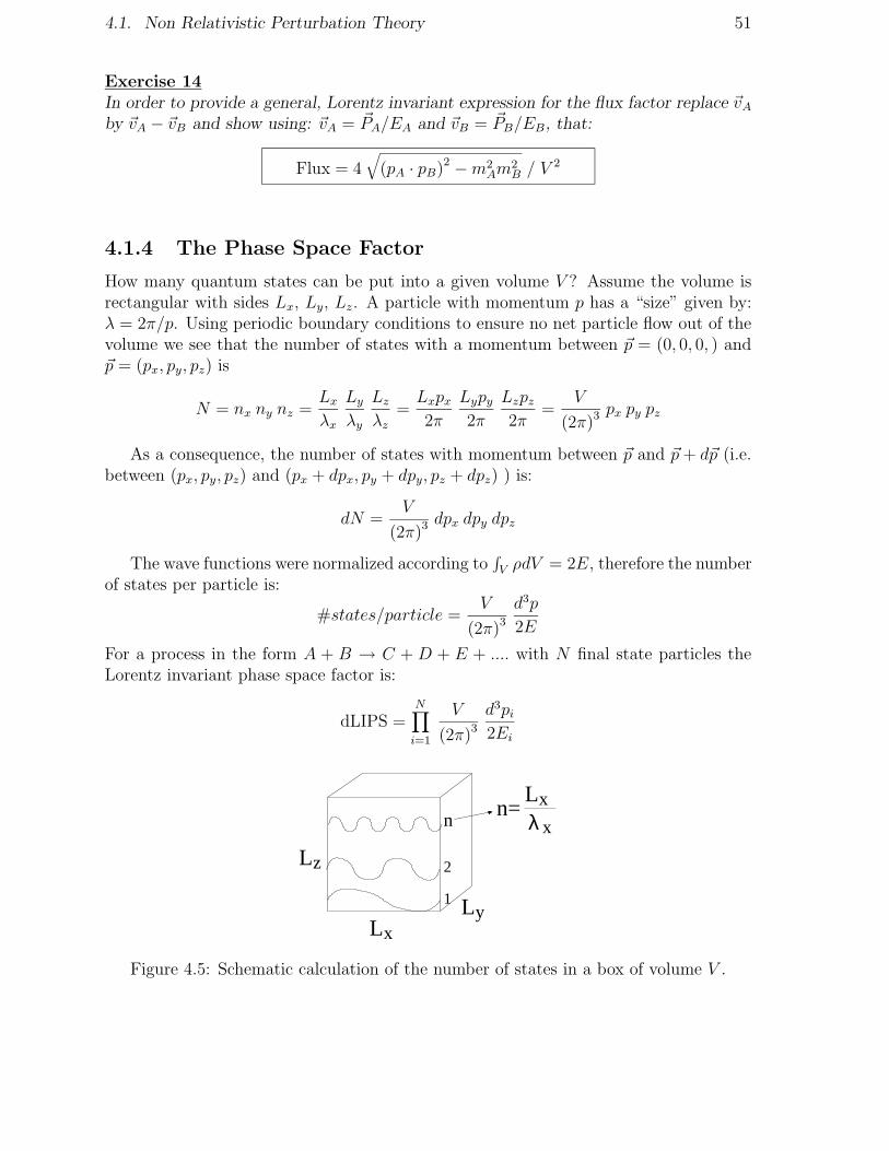
How many quantum states can be put into a given volume V ? Assume the volume isrectangular with sides Lx, Ly, Lz. A particle with momentum p has a “size” given by:λ = 2π/p. Using periodic boundary conditions to ensure no net particle flow out of thevolume we see that the number of states with a momentum between ~p = (0, 0, 0, ) and~p = (px, py, pz) is
N = nx ny nz =Lxλx
Lyλy
Lzλz
=Lxpx2π
Lypy2π
Lzpz2π
=V
(2π)3px py pz
As a consequence, the number of states with momentum between ~p and ~p+ d~p (i.e.between (px, py, pz) and (px + dpx, py + dpy, pz + dpz) ) is:
dN =V
(2π)3dpx dpy dpz
The wave functions were normalized according to∫
V ρdV = 2E, therefore the numberof states per particle is:
#states/particle =V
(2π)3d3p
2E
For a process in the form A + B → C + D + E + .... with N final state particles theLorentz invariant phase space factor is:
dLIPS =N∏
i=1
V
(2π)3d3pi2Ei
n
LxL
L
y
z
1
2
Lxλ x
n=
Figure 4.5: Schematic calculation of the number of states in a box of volume V .
52 Lecture 4. Perturbation Theory and Fermi’s Golden Rule
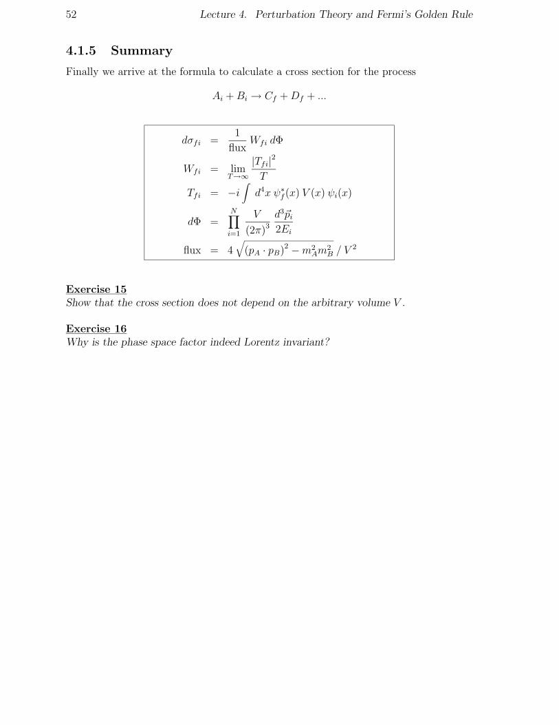
4.1.5 Summary
Finally we arrive at the formula to calculate a cross section for the process
Ai +Bi → Cf +Df + ...
dσfi =1
fluxWfi dΦ
Wfi = limT→∞
|Tfi|2T
Tfi = −i∫
d4x ψ∗f (x) V (x) ψi(x)
dΦ =N∏
i=1
V
(2π)3d3~pi2Ei
flux = 4√
(pA · pB)2 −m2Am
2B / V
2
Exercise 15Show that the cross section does not depend on the arbitrary volume V .
Exercise 16Why is the phase space factor indeed Lorentz invariant?

4.2. Extension to Relativistic Scattering 53
4.2 Extension to Relativistic Scattering
The transition amplitude of the scattering process A + B → C +D, for incoming andoutgoing plane waves φ = Ne−ipx takes the form:
Tfi = −i NANBNCND (2π)4 δ(pA + pB − pC − pD)M
whereM is the so-called Matrix element and the delta function takes care of the energyand momentum conservation in the process.
To find the transition probability we square this expression:
|Tfi|2 = |NANBNCND|2∫
d4x e−i(pA+pB−pC−pD)x ×∫
d4x′ e−i(pA+pB−pC−pD)x′
= |NANBNCND|2 (2π)4 δ4(pA + pB − pC − pD)× limT,V→∞
∫
TVd4x
= |NANBNCND|2 (2π)4 δ4(pA + pB − pC − pD)× limT,V→∞
TV
This gives for the transition probability per unit time and volume:
Wfi = limT,V→∞
|Tfi|2TV
= |NANBNCND|2 |M|2 (2π)4 δ (pA + pB − pC − pD)
Indeed we see that the delta funtion provides conservation of energy and momentum.
The cross section is again given by1:
dσ =Wfi
FluxΦ2
The phase space factor is:
Φ2 =V d3pC
(2π)3 · 2EC
V d3pD(2π)3 · 2ED
and the Flux factor is:
Flux = 4√
(pA · pB)2 −m2A m
2B / V
2
Taking it all together with N = 1√V :
dσ =1
V 4|M|2 (2π)4δ4 (pA + pB − pC − pD)·
V 2
4√
(pA · pB)2 −m2Am
2B
· V d3pC
(2π)3 2EC
V d3pD
(2π)3 2ED
In this formula the arbitrary volume factors V cancel again.
1Usually we will write this as:
dσ =|M|2Flux
dΦ
and absorb the delta function in the phase space factor.

54 Lecture 4. Perturbation Theory and Fermi’s Golden Rule
We finally have for the cross section of A+B → C +D:
dσ =(2π)4 δ4 (pA + pB − pC − pD)
4√
(pA · pB)2 −m2Am
2B
· |M|2 · d3pC
(2π)3 2EC
d3pD
(2π)3 2ED
Similarly the formula for decay A→ C +D is:
dΓ =(2π)4 δ4 (pA − pC − pD)
2EA
· |M|2 · d3pC
(2π)3 2EC
d3pD
(2π)3 2ED
Exercise 17Calculate the two particle phase space in the interaction A+B → C +D.
(a) Start with the expression:
Φ2 =∫
(2π)4 δ4 (pA + pB − pC − pD)d3 ~pC
(2π)3 2EC
d3 ~pD
(2π)3 2ED
Do the integral over d3pD using the δ function and show that we can write:
Φ2 =∫ 1
(2π)2p2f dpf dΩ
4ECED
δ (EA + EB − EC − ED)
where we have made use spherical coordinates (i.e.: d3pC = |pC |2dpC dΩ) and ofpf ≡ |pC |, .
(b) In the C.M. system we can write:√s ≡ W = EA+EB. Show that the expression
becomes:
Φ2 =∫ 1
(2π)2pf4
(1
EC + ED
)
dW dΩ δ (W − EC − ED)
So that we finally get:
Φ2 =1
4π2pf4√sdΩ
(c) Show that the flux factor in the center of mass is:
F = 4pi√s
and hence that the differential cross section for a 2 → 2 process in the center ofmass frame is given by:
dσ
dΩ
∣∣∣∣∣cm
=1
64π2s
pfpi|M|2
Lecture 5
Electromagnetic Scattering ofSpinless Particles
Introduction
In this lecture we discuss electromagnetic scattering of spinles particles. First we de-scribe an example of a charged particle scattering in an external electric field. Secondwe derive the cross section for two particles that scatter in each-others field. We endthe lecture with a prescription how to treat antiparticles.
5.1 Electrodynamics
How do we introduce electrodynamics in the wave equation of a system? The freeLagrangian of a free particle is:
L = T − V =1
2m~v2
In the presence of an electromagnetic field the equation of movement is:
~F =d~p
dt= q
(
~E + ~v × ~B)
The Lagrangian that leads to the desired equation of motion is (see e.g. Jackson):
L =1
2m~v2 + q~v · ~A(~r, t)
︸ ︷︷ ︸
T
− qΦ(~r, t)︸ ︷︷ ︸
V
This means that we replace the kinematic energy and momentum by the canonicalenergy and momentum: E → E + qΦ and ~p =→ ~p+ q ~A1. In 4-vec notation:
pµ → pµ + qAµ
This is called minimal substitution contains the essential physics of electrodynamics.
1Note that: ∂L∂v= mv + qA
55

56 Lecture 5. Electromagnetic Scattering of Spinless Particles
Exercise 18A charged particle moves in a uniform static magnetic field ~B.
(a) Show that for a uniform magnetic field, we may take:
V = 0, ~A =1
2~B × ~r
If we choose the z-axis in the direction of ~B we have in cylindrical coordinates(r, φ, z):
V = 0, Ar = 0, Aφ =1
2Br, Az = 0
Hint: In cylindrical coordinates the cross product is defined as:
~∇× ~A =
(1
r
∂Az
∂φ− ∂Aφ
∂z,∂Az
∂z− ∂Az
∂r,1
r
[∂ (rAφ)
∂r− ∂Ar
∂φ
])
(b) Write down the Lagrangian in cylindrical coordinates
(c) Write out the Lagrangian equations:
d
dt
(
∂L∂qα
)
=∂L∂qα
in the cylindrical coordinates.
(d) Show that the equation of motion in terms of the coordinate φ yields (assumer=constant):
φ = 0 or φ = −qBm
i.e. that it is in agreement with the law:
~F =d~p
dt= q
(
~E + ~v × ~B)
In quantum mechanics we make the replacement pµ → i∂µ, such that we have now:
∂µ → ∂µ − iqAµ
This is the heart of quantum electrodynamics. As we will see later in the lectures thissubstitution is mandatory in order make the the theory quantum electrodynamics locallygauge invariant!
Start with the free particle Klein-Gordon equation:
(
∂µ∂µ +m2
)
φ = 0

5.1. Electrodynamics 57
and substitute ∂µ → ∂µ − ieAµ:
(∂µ − ieAµ) (∂µ − ieAµ) φ+m2φ = 0
which is of the form: (
∂µ∂µ +m2 + V (x)
)
φ = 0
from which we derive for the perturbation potential:
V (x) = −ie (∂µAµ + Aµ∂µ)− e2A2
Since e2 is small (α = e2/4π = 1/137) we can neglect the second order term: e2A2 ≈ 0.
φ
H
V(x,t)i
f
0
0H
φ
Figure 5.1: Scattering potential
From the previous lecture we take the general expression for the transition amplitude:
Tfi = −i∫
d4x φ∗f (x) V (x) φi(x)
= −i∫
d4x φ∗f (x) (−ie) (Aµ∂µ + ∂µA
µ) φi(x)
Use now partial integration to calculate:
∫
d4x φ∗f ∂µ (Aµ φi) =
[
φ∗f Aµ φi
]∞
−∞︸ ︷︷ ︸
=0
−∫
∂µ
(
φ∗f)
Aµ φi d4x
note that at t = −∞ and at t = +∞: Aµ = 0.
We then get:
Tfi = −i∫
−ie[
φ∗f (x) (∂µφi(x))−(
∂µφ∗f (x)
)
φi(x)]
︸ ︷︷ ︸
jfiµ
Aµ d4x
We had the definition of a Klein-Gordon current density:
jµ = −ie [φ∗ (∂µφ)− (∂µφ∗)φ]
58 Lecture 5. Electromagnetic Scattering of Spinless Particles
In complete analogy we now define the “transition current density” to go from initialstate i to final state f :
jfiµ = −ie[
φ∗f (∂µφi)−(
∂µφ∗f
)
φi]
so that we arrive at:
Tfi = −i∫
jfiµ Aµ d4x
This is the expression for the transition amplitude for going from free particle solution ito free particle solution f in the presence of a perturbation caused by an electromagneticfield.
If we substitute the free particle solutions of the unperturbed Klein-Gordon equationin initial and final states we find for the transition current of spinless particles:
φi = Ni e−ipix ; φ∗f = N∗
f eipfx
jfiµ = −eNiN∗f
(
piµ + pfµ)
ei(pf−pi)x
5.2 Scattering in an External Field
Consider the case that the external field is a static field of a point charge Z located inthe origin:
Aµ =(
V, ~A)
=(
V,~0)
with V (x) =Ze
|~x|The transition amplitude is:
Tfi = −i∫
jµfi Aµ d4x
= −i∫
(−e)NiN∗f
(
pµi + pµf)
Aµ ei(pf−pi)x d4x
Insert that Aµ =(
V,~0)
and thus: pµ Aµ = E V :
Tfi = i∫
eNiN∗f (Ei + Ef ) V (x) ei(pf−pi)x d4x
Split the integral in a part over time and in a part over space and note that V (~x) is not
time dependent. Use also again:∫
ei(Ef−Ei)tdt = 2π δ (Ef − Ei) to find that:
Tfi = ieNiN∗f (Ei + Ef ) 2π δ (Ef − Ei)
∫ Ze
|~x| e−i(~pf−~pi)~x d3x
Now we make use of the Fourier transform:
1
|~q|2 =∫
d3x ei~q~x1
4π|~x|
5.2. Scattering in an External Field 59
Using this with ~q ≡ (~pf − ~pi) we obtain:
Tfi = ieNiN∗f (Ei + Ef ) 2π δ (Ef − Ei)
4πZe
|~pf − ~pi|2
The next step is to calculate the transition probability:
Wfi = limT→∞
|Tfi|2T
= limT→∞
1
T
∣∣∣NiN
∗f
∣∣∣ [2π δ (Ef − Ei)]
2
(
4πZe2 (Ei + Ef )
|~pf − ~pi|2)2
We apply again our “trick”:
limT→∞
[2π δ (Ef − Ei)]2 = 2π δ (Ef − Ei) · lim
T→∞
∫ T/2
−T/2dt ei(Ef−Ei)t
= 2π δ (Ef − Ei) · limT→∞
∫ T/2
−T/2ei0tdt
︸ ︷︷ ︸
T
= limT→∞
2π δ (Ef − Ei) · T
Putting this back into Wfi we obtain:
Wfi = limT→∞
1
T· T |NiNf |2 2π δ (Ef − Ei)
(
4πZe2 (Ei + Ef )
|~pf − ~pi|2)2
The cross section is given by:
dσ =Wfi
FluxdLips
with :
Flux2 = ~v2Ei
V=~piEi
2Ei
V=
2~piV
dLips =V
(2π)3d3pf2Ef
Normalization : N =1√V
→∫
Vφ∗φdV = 1
In addition from energy and momentum conservation we write E = Ei = Ef andp = |~pf | = |~pi|
Putting everything together:
dσ =1
V 22π δ (Ef − Ei) ·
(
4πZe2 (Ei + Ef )
|~pf − ~pi|2)2
· V
2 |~pi|V
(2π)3d3pf2Ef

60 Lecture 5. Electromagnetic Scattering of Spinless Particles
Note that the arbitrary volume V drops from the expression!Use now d3pf = p2f dpf dΩ and |pf | = |pi| = p to get:
dσ =1
(2π)2δ (Ef − Ei)
(
4πZe2 (Ei + Ef )
|~pf − ~pi|2)2 p2f dpf dΩ
2|~pi| 2Ef
= δ (Ef − Ei)
4Ze2 (Ei + Ef )
2p2 (1− cos θ)︸ ︷︷ ︸
4p2 sin2 θ/2
2
p dp dΩ
4E
now use p dp = E dE such that:
p dp dΩ
4Eδ (Ef − Ei) =
dE δ (Ef − Ei) dΩ
4=dΩ
4
We arrive at the expression for the differential cross section:
dσ =
(
Ze2E
2p2 sin2 θ/2
)2
dΩ
or:
dσ
dΩ=
Z2E2e4
4p4 sin4 θ/2=
Z2E2α2
4p4 sin4 θ/2
In the classical (i.e. non-relativistic) limit we can take E → m and Ekin = p2
2msuch
that:dσ
dΩ=
Z2m2α2
16m2E2 sin4 θ/2=
Z2α2
16E2 sin2 θ/2
the well known Rutherford scattering formula.
5.3 Spinless π −K Scattering
Let us proceed to the case of QED scattering of a π− particle on a K− particle. Weignore the fact that pions and kaons also are subject to the strong interaction (e.g. wecould consider scattering at large distances).
Aµ γ
A : π−
B : K−
C : π−
D : K−
We know from the previous calculation how aparticle scatters in an external field. In this casethe field is not external as the particles scatterin each others field. How do we deal with it?

5.3. Spinless π −K Scattering 61
Ansatz:Consider first only the pion. It scatters in the field of the kaon. How do we find the fieldgenerated by the kaon? This field is again caused by the transition current jµBD of thescattering kaon. The field is then found by solving Maxwell’s equations for this current(adopting the Lorentz gauge condition):
∂ν∂νAµ = jµBD = −eNBN
∗D (pµB + pµD) e
i(pD−pB)x
(see the previous section.)Since ∂ν∂
νe−iqx = −q2 e−iqx we can verify that
Aµ =e
q2NBN
∗D (pµB + pµD) e
i(pD−pB)x = − 1
q2jµBD
where we have used that q = (pD− pB) = −(pC − pA) is the 4-vector momentum that istransmitted from the pion particle to the kaon particle via the Aµ field, i.e. the photon.
In this case the transition amplitude becomes:
Tfi = −i∫
jµAC Aµ d4x = −i
∫
jµAC−1q2jBDµ d4x = −i
∫
jµAC−gµνq2
jνBD d4x
Note:
1. The expression is symmetric in the two currents. It does not matter whether wescatter the pion in the field of the kaon or the kaon in the field of the pion.
2. There is only scattering if q2 6= 0. This is interesting as for a “normal” photonone has q2 = m2 = 0. It implies that we deal with virtual photons; i.e. photonsthat are “off mass-shell”.
Writing out the expression we find:
Tfi = −ie2∫
(NAN∗C) (pµA + pµC) e
i(pC−pA)x · 1q2· (NBN
∗D) (pµB + pµD) e
i(pB−pD)x
Next, do the integrals over x in order to obtain the energy-momentum conservationδ-functions:
Tfi = −ie2 (NAN∗C) (pµA + pµC)
1
q2(NBN
∗D)
(
pBµ + pDµ)
(2π)4 δ4 (pA + pB − pC − pD)
Usually this is written in terms of the matrix element M as:
Tfi = −i NANBN∗CN
∗D (2π)4 δ4 (pA + pB − pC − pD) · M
with : M = ie (pA + pC)µ
︸ ︷︷ ︸
vertex factor
· −igµνq2
︸ ︷︷ ︸
propagator
· ie (pB + pD)ν
︸ ︷︷ ︸
vertex factor

62 Lecture 5. Electromagnetic Scattering of Spinless Particles
−igµνq2
A
B
C
D
ie(pA + pC)µ
ie(pB + pD)µ
The matrix element M contains:
a vertex factor: for each vertex we introduce thefactor: iepµ, where:· e is the intrinsic coupling strength of the par-ticle to the e.m. field.· pµ is the sum of the 4-momenta before and af-ter the scattering (remember the particle/anti-particle convention).
a propagator: for each internal line we introduce afactor −igµν
q2, where:
· q is the 4-momentum of the exchanged photonquantum.
Using Fermi’s golden rule we can proceed to calculate the relativistic transitionprobability:
Wfi = limT,V→∞
|Tfi|2TV
= limT,V→∞
1
TV|NANBN
∗CN
∗D|2 |M|2
∣∣∣(2π)4δ4 (pA + pB − pC − pD)
∣∣∣
2
Again we use the “trick” :
δ(p) = limT,V→∞
1
(2π)4
∫ +T/2
−T/2dt
∫ +V/2
−V/2d3x eipx
such that
limT,V→∞
1
TV|δ4(p)|2 = 1
TVTV δ(p)
We get for the transition amplitude:
Wfi = |NANBNCND|2 |M| (2π)4 δ4 ((pA + pB − pC − pD)
For the scattering process: A+B → C +D the cross section is obtained from:
dσ =Wfi
FluxdLips
Flux = 4√
(pA · pB)2 −m2Am
2B/V
2
dLips =V
(2π)3d3pC2EC
V
(2π)3d3pD2ED
The volume V cancels again and we obtain:
dσ =(2π)4 δ4 (pA + pB − pC − pD)
4√
(pA · pB)2 −m2Am
2B
|M|2 d3pC
(2π)3 2EC
d3pD
(2π)3 2ED

5.3. Spinless π −K Scattering 63
which leads to the differential cross section for 2→ 2 electromagnetic scattering is (seeexercise 17)’:
dσ
dΩ=
1
64π21
s
∣∣∣∣∣
~pf~pi
∣∣∣∣∣|M|2
We will work it out for the relativistic case that: E = p, i.e. m ≈ 0.
pµA = (p, p, 0, 0)
pµB = (p,−p, 0, 0)pµC = (p, p cos θ, p sin θ, 0)
pµD = (p,−p cos θ,−p sin θ, 0)qµ = (pD − pB)
µ = (0, p(1− cos θ),−p sin θ, 0)
pC
pB
Ap
pD
q2θ
We calculate the matrix element and the differential cross section using:
(pA + pC)µ = (2p, p(1 + cos θ), p sin θ, 0)
(pB + pD)µ = (2p,−p(1 + cos θ),−p sin θ, 0)
to get:
(pA + pC)µ gµν (pB + pD)
ν = p2 (6 + 2 cos θ)
q2 = −2p2 (1− cos θ)
We then find for the matrix element:
−iM = e (pA + pC)µ gµνq2
e (pB + pD)µ
= e2p2 (6 + 2 cos θ)
2p2 (1− cos θ)= e2
(
3 + cos θ
1− cos θ
)
and then:
|M|2 =(
e2)2(
3 + cos θ
1− cos θ
)2
Finally we obtain from:dσ
dΩ=
1
64π21
s
p
p|M|2
the cross section (α = e2/4π):
dσ
dΩ=
1
64π21
s
(
e2)2(
3 + cos θ
1− cos θ
)2
=α2
4s
(
3 + cos θ
1− cos θ
)2
This is the QED cross section for spinless scattering.

64 Lecture 5. Electromagnetic Scattering of Spinless Particles
5.4 Particles and Anti-Particles
We have seen that the negative energy state of a particle can be interpreted as thepositive energy state of its anti-particle. How does this effect energy conservation thatwe encounter in the δ-functions? We have seen that the Matrix element has the formof:
M∝∫
φ∗f (x) V (x) φi(x) dx
Let us examine four cases:
• Scattering of an electron and a photon:
k
pi
pf
M ∝∫
e−ipix e−ikx(
e−ipfx)∗
dx
=∫
e−i(pi+k−pf)x dx
= (2π)4 δ (Ei + ω − Ef ) δ3(
~pi + ~k − ~pf)
⇒ Energy and momentum conservation areguaranteed by the δ-function.
• Scattering of a positron and a photon:
k
−pi
−pf
Replace the anti-particles always by particles byreversing (E, ~p→ −E,−~p) such that now:incoming state = −pf , outgoing state = −pi:
M ∝∫
e−i(−pf )x e−ikx(
e−i(−pi)x)∗
dx
=∫
e−i(pi−pf+k)x dx
= (2π)4 δ (Ei + ω − Ef ) δ3(
~pi + ~k − ~pf)
• Electron positron pair production:
k
p−
-p+
M ∝∫
e−i(−p++k)x(
e−ip−x)∗
dx
=∫
e−i(k−p+−p−)x dx
= (2π)4 δ (k − p− − p+)
• Electron positron annihilation:
-p+
p−
k M ∝∫
e−i(p−)x(
e−i(k−p+)x)∗
dx
=∫
e−i(p−+p+−k)x
= (2π)4 δ (p− + p+ − k)
5.4. Particles and Anti-Particles 65
Exercise 19Decay rate of π0 → γγ:
(a) Write down the expression for the total decay rate Γ for the decay: A→ C +D
(b) Assume that particle A is a π0 particle with a mass of 140 MeV and that particlesC and D are photons. Draw the Feynman diagram for this decay assuming thepion is a uu state.
(c) For the Matrix element we have: M ∼ fπ e2, where for the decay constant we
insert fπ = mπ.
(i) Where does the factor e2 come from?
(ii) What do you think is the meaning of the factor fπ? Describe it qualitatively.
(d) (i) Calculate the decay rate expressed in GeV.
(ii) Convert the rate into seconds using the conversion table of the introductionlecture.
(iii) How does the value compare to the Particle Data Group (PDG) value?

66 Lecture 5. Electromagnetic Scattering of Spinless Particles

Lecture 6
The Dirac Equation
Introduction
It is sometimes said that Schrodinger had first discovered the Klein-Gordon equationbefore the equation carrying his own name, but that he had rejected it because it wasquadratic in ∂
∂t. In Lecture 2 we have seen how indeed the Klein-Gordon equation leads
to the interpretation of negative probabilities: ρ = 2|N |2E, where the energy can be:E = ±
√~p2 +m2.
To avoid this problem Dirac in 1928 tried to make a relativistic correct equation thatwas linear in ∂
∂t. He wanted to combine the merits of a linear combination (no negative
probabilites) with the relativistic correctness of the K.G. equation. Since he wanted the
equation to be linear in ∂∂t, Lorentz covariance requires it to be also linear in ~∇.
What Dirac found, to his own great surprise, was an equation that describes particleswith spin 1
2, i.e. the fundamental fermions. At the same time he predicted the existence
of anti-matter. This was not taken serious untill 1932, when Anderson found the anti-electron: the positron.
6.1 Dirac Equation
Write the Hamiltonian in a general form1:
Hψ = (~α · ~p+ βm) ψ (6.1)
with coefficients α1, α2, α3, β. These must be chosen such that after squaring one finds:
H2ψ =(
~p2 +m2)
ψ
Let us try eq 6.1 and see what happens:
H2ψ = (αipi + βm)2 ψ with : i = 1, 2, 3
=
α2i︸︷︷︸
=1
p2i + (αiαj + αjαi)︸ ︷︷ ︸
=0 i>j
pipj + (αiβ + βαi)︸ ︷︷ ︸
=0
pim+ β2︸︷︷︸
=1
m
ψ
1Here ~α · ~p = αxpx + αypy + αzpz
67
68 Lecture 6. The Dirac Equation
So we have the following requirements:
• α21 = α22 = α23 = β2 = 1
• α1, α2, α3, β anti-commute with each other.
Note that Dirac discovered this just a few years after the beginning of the formulation of
quantum mechanics and commuting operators. He was highly interested in the mathematical
behaviour of the operators.
Immediatly we conclude that ~α, β cannot be ordinary numbers, but that they mustbe matrices. They now operate on a wave function which has become a column vector(called a spinor). This was not believed when Dirac first published his theory.
The lowest dimensional matrices that have the desired behaviour are 4× 4 matrices(see the book of Aitchison (1972) chapter 8; section 1). The choice of the (~α, β) ishowever not unique. Here we choose the Dirac-Pauli representations:
~α =
(
0 ~σ~σ 0
)
; β =
(
I 00 −I
)
where ~σ are the Pauli matrices:
σ1 =
(
0 11 0
)
; σ2 =
(
0 −ii 0
)
; σ3 =
(
1 00 −1
)
Note that the physics is independent of the representation. It only depends on theanti-commuting behaviour of the operators. Another representation is the Weyl repre-sentation:
~α =
(
−~σ 00 ~σ
)
; β =
(
0 II 0
)
Exercise 20Show that the ~α and β matrices in both the Dirac-Pauli as well as in the Weyl repre-sentation have the required anti-commutation behaviour.
One can show using the fact that the energy must be real (see Aitchison) that theαi and β matrices are Hermitian:
α†i = αi ; β† = β
6.2 Covariant form of the Dirac Equation
We hadHψ = (~α · ~p+ βm) ψ

6.2. Covariant form of the Dirac Equation 69
Now we replace: H → i ∂∂t, ~p→ −i~∇ to find:
i∂
∂tψ =
(
−i~α · ~∇+ βm)
ψ
Multiply this equation from the left side by β (note that β2 = 1):
iβ∂
∂tψ = −iβ~α · ~∇+mψ
iβ∂
∂tψ + iβ~α · ~∇ψ −mψ = 0
(
iβ∂
∂tψ + iβα1
∂
∂x+ iβα2
∂
∂y+ iβα3
∂
∂z
)
ψ −mψ = 0
in which we see a nice symmetric structure arising. We write the equation in a covariantnotation:
(iγµ∂µ −m) ψ = 0
with : γµ = (β, β~α) ≡ Dirac γ−matrices
In fact the Dirac eq. are really 4 coupled differential equations:
for eachj=1,2,3,4
:4∑
k=1
3∑
µ=0
i (γµ)jk ∂µ −mδjk
(ψk) = 0
or :
i
. . . .
. . . .
. . . .
. . . .︸ ︷︷ ︸
γµ
· ∂µ −
1 0 0 00 1 0 00 0 1 00 0 0 1
·m
ψ1ψ2ψ3ψ4
=
0000
or even more specific:
[(
11 00 −11
)
i∂
∂t+
(
0 σ1−σ1 0
)
i∂
∂x+
(
0 σ2−σ2 0
)
i∂
∂y+
(
0 σ3−σ3 0
)
i∂
∂z−(
11 00 11
)
m
]
ψ1ψ2ψ3ψ4
=
0000
Take note of the use of the Dirac (or spinor) indices (k = 1, 2, 3, 4) simultaneously withthe Lorentz indices (µ = 0, 1, 2, 3).
On the other hand, there is an alternative and very short notation: an electron isdescribed by:
(iγµ∂µ −m)ψ = 0 ⇒ (i 6∂ −m)ψ = 0
while the equation:i 6∂ ψ = 0
contains everything you want to know about a neutrino (assuming m = 0).

70 Lecture 6. The Dirac Equation
6.3 The Dirac Algebra
From the definitions of ~α and β we can derinve the following relation:
γµγν + γνγµ ≡ γµ, γν = 2gµν
Thus: (
γ0)2
= 11 ;(
γ1)2
=(
γ2)2
=(
γ2)2
= −11Also we have the Hermitean conjugates:
γ0†
= γ0 ; β† = β
γi†
=(
βαi)†
= αi†β† = αiβ = −γi
Then the relation
γk, γ0
= 0 implies:
γkγ0 = −γ0γk = γ0γk†
thus : γ0γkγ0 = γ02γk†= γk
†
In general:
㵆 = γ0γµγ0
In words this means that we can undo a hermitean conjugate 㵆γ0 by moving a γ0
“through it”: 㵆γ0 = γ0γµ
Furthermore we can define:
γ5 = iγ0γ1γ2γ3 =
(
0 1111 0
)
with the characteristics:
γ5†= γ5
(
γ5)2
= 11
γ5, γµ
= 0
6.4 Current Density
Similarly to the case of the Schrodinger and the Klein-Gordon equations we can derivea continuity equation to determine the current density jµ: Write the Dirac equation as:
iγ0∂ψ
∂t+ iγk
∂ψ
∂xk−mψ = 0 k = 1, 2, 3
We work now with matrices, so instead of complex conjugates we use Hermitean conju-gates:
−i∂ψ†
∂tγ0 − i
∂ψ†
∂xk
(
−γk)
−mψ† = 0

6.4. Current Density 71
But now we have a problem! The additional − sign in(
−γk)
disturbs the Lorentzinvariant form of the equation. This means we cannot use this equation.We can restore Lorentz covariance by multiplying the equation form the right by γ0.Or, in other words, we can define the adjoint spinor as: ψ = ψ†γ0.
Dirac spinor :
ψ1ψ2ψ3ψ4
Adjoint Dirac spinor :(
ψ1, ψ2, ψ3, ψ4)
The adjoint Dirac equation the becomes:
−i∂ψ∂tγ0 − i
∂ψ
∂xkγk −mψ = 0 k = 1, 2, 3
Now we multiply the Dirac equation from the left by ψ and we mulitply the adjointDirac equation from the right by ψ:
(
i∂µψγµ +mψ
)
ψ = 0
ψ (i∂µγµψ −mψ) = 0
+
ψ (∂µγµψ) +
(
∂µψγµ)
ψ = 0
We recognize again the continuity equation:
∂µjµ = 0 with : jµ =
(
ψγµψ)
6.4.1 Dirac Interpretation
Consider
j0 = ψγ0ψ = ψ†γ0γ0ψ = ψ†ψ =4∑
i=1
|ψi|2 > 0
Therefore the probability density is always greater then 0! This is the historical moti-vation of Dirac’s work.
However, we had seen in the Pauli-Weiskopf interpretation that jµ =(
ρ,~j)
was thecharge current density. In that case:
jµ = −eψγµψis the electric 4-vector current density (just as we used it before). The − sign meansthat the electron is considered to be the particle and the positron the anti-particle.
If we use the ansatz: ψ = u(p)e−ipx for the spinor ψ then we get for the interactioncurrent density 4-vector:
jµfi = −eu†fγ0γµuiei(pf−pi)x
= −eufγµuie−iqx
jµfi = −e ( uf )
γµ
ui
· e−iqx
72 Lecture 6. The Dirac Equation
Exercise 21: Traces and products of γ matricesFor the γ matrices we have:
γµγν + γνγµ = 2 gµν
Use this relation to show that:
(a) 6a 6b+ 6b 6a = 2 (a · b)
(b) i) γµγµ = 4
ii) γµ 6a γµ = −2 6aiii) γµ 6a 6b γµ = 4 (a · b)iv) γµ 6a 6b 6c γµ = −2 6c 6b 6a
(c) i) Tr 11 = 4
ii) Tr (odd number of γµ’s) = 0
iii) Tr (6a 6b ) = 4 (a · b)iv) Tr (6a 6b 6c 6d ) = 4 [ (a · b)(c · d)− (a · c)(b · d) + (a · d)(b · c) ]
(d) i) Tr γ5 = Tr i γ0γ1γ2γ3 = 0
ii) Tr γ5 6a 6b = 0
iii) Tr γ5 6a 6b 6c 6d = 4 i εαβγδ aαbβcγdδ
where εαβγδ = +1(−1) for an even (odd) permutation of 0,1,2,3; and 0 if twoindices are the same.

Lecture 7
Solutions of the Dirac Equation
7.1 Solutions for plane waves with ~p = 0
We look for free particle solutions of:
(iγµ∂µ −m) ψ = 0
Exercise 22Each of the four components of the Dirac equation satisfies the Klein Gordon equation:(∂µ∂
µ +m2)ψi = 0.Show this explicitly by operating on the Dirac equation from the left with: γν∂ν .Hint: Use the anticommutation relation of the γ-matrices.
Ansatz:This suggests to try the plane wave solutions:
ψ(x) = u(p) e−ipx
Since ψ(x) is a 4-component spinor, also u(p) is a 4-component spinor. After substitutionwe find, what is called the Dirac equation in the momentum representation:
(γµpµ −m) u(p) = 0
or : (6p −m) u(p) = 0
Remember that the Dirac equation is a linear set of equations (use here the Pauli-Diracrepresentation):
[ (
11 00 −11
)
E −(
0 σi−σi 0
)
pi −(
11 00 11
)
m
] (
uAuB
)
= 0
In fact we can recognize two coupled equations:
(~σ · ~p) uB = (E −m)uA(~σ · ~p) uA = (E +m)uB
73

74 Lecture 7. Solutions of the Dirac Equation
where uA and uB are now each two component spinors.Let us first look at solutions for a particle at rest: ~p = 0:
(~σ · ~p) uB = (E −m)uA(~σ · ~p) uA = (E +m)uB
⇒
E uA = m uAE uB = −m uB
For these equations there are 4 independent solutions, the eigenvectors:
u(1) =
1000
, u(2) =
0100
, u(3) =
0010
, u(4) =
0001
with eigenvalues: E = m, m, −m, −m, respectively.u(1), u(2) are the positive energy solutions of e−.u(3), u(4) are the negative energy solutions of e− and thus the positive energy solutionsof e+.
We define:
v(1)(p) = u(4)(−p)v(2)(p) = −u(3)(−p)
7.2 Solutions for moving particles ~p 6= 0
Again look at:
(~σ · ~p) uB = (E −m)uA(~σ · ~p) uA = (E +m)uB
Choose now for the two E > 0 solutions:
u(1)A =
(
10
)
, u(2)A =
(
01
)
Then it follows:
u(1)B =
~σ · ~pE +m
u(1)A =
~σ · ~pE +m
(
10
)
u(2)B =
~σ · ~pE +m
u(2)A =
~σ · ~pE +m
(
01
)
So, the two independent solutions are:
u(1) =
(
u(1)A
u(1)B
)
, u(2) =
(
u(2)A
u(2)B
)
Analogously: choose for the two E < 0 solutions:
u(3)B =
(
10
)
, u(4)B =
(
01
)

7.2. Solutions for moving particles ~p 6= 0 75
then it follows:
u(3)A =
~σ · ~pE −m
u(3)B = − ~σ · ~p
|E|+m
(
10
)
u(4)A =
~σ · ~pE −m
u(4)B = − ~σ · ~p
|E|+m
(
01
)
So, the two independent solutions are now:
u(3) =
(
u(3)A
u(3)B
)
, u(4) =
(
u(4)A
u(4)B
)
To gain insight, let us write them out in more detail.Use the explicit representation:
~σ · ~p =(
0 11 0
)
px +
(
0 −ii 0
)
py +
(
1 00 −1
)
pz
we find:
(~σ · ~p) u(1)A =
(
pz px − ipypx + ipy −pz
) (
10
)
=
(
pzpx + ipy
)
and similar for u(2)A , u
(3)B , u
(4)B .
Then we find the solutions:
electron spinors : u(1) = N
10pz
E+mpx+ipyE+m
, u(2) = N
01
px−ipyE+m−pzE+m
positron spinors : v(1) = N
px−ipy|E|+m−pz|E|+m01
, v(2) = N
−pz|E|+m
−(px+ipy)|E|+m−10
and we can verify that the u(1) - u(4) solutions are indeed orthogonal.
Exercise 23Show explicitly that the Dirac equations describes relativistic particles. To do thissubstitute the expression:
uB =~σ · ~pE +m
uA into uA =~σ · ~pE −m
uB
Hint: Work out the product (~σ · ~p)2 in components.

76 Lecture 7. Solutions of the Dirac Equation
7.3 Particles and Anti-particles
The spinors u(p) of matter waves are solutions of the Dirac equation:
(6p −m) u(p) = 0 ⇒ solutions with p0 = E > 0
For the antiparticles (the solutions v(p)) we have substituted v(p) = u(−p). Rememberthat we interpret an antiparticle as a particle travelling back in time. Let us make thesame substitution in the Dirac equation (for negative p0 !):
(− 6p −m) u(−p) = 0 ⇒ replaced p→ −pThen we find for solutions with the new p0 (=E>0) the Dirac equation for anti-particles:
(6p +m) v(p) = 0
7.4 Normalisation
We choose again (similar to the Klein-Gordon case) a normalisation of the wave functionsuch that there are 2E particles in a unit volume:
∫
VρdV =
∫
ψγ0ψ dV =∫
ψ†γ0γ0ψdV =∫
ψ†ψdV
Substitute now the plane wave solution: ψ = u(p) e−ipx:∫
ρdV =∫
u†(p) eipx u(p) e−ipx dV = u†(p)u(p)∫
VdV
Choose the unit volume and normalise to 2E:∫
VdV = 1 ; u†(p)u(p) = 2E
where for u we must substitute: u1(p), u2(p), v1(p), v2(p). Using orthogonality of thesolutions we get the relations:
u(r)†u(s) = 2E δrs r, s = 1, 2
v(r)†v(s) = 2E δrs r, s = 1, 2
Explicit calculation gives:
u(1)†u(1) = N2
(
1, 0,pz
E +m,px − ipyE +m
)
10pz
E+mpx+ipyE+m
= 2E
..... ⇒ N2
(E +m)2
(E +m)2 + p2x + p2y + p2z
︸ ︷︷ ︸
E2−m2
= 2E
..... ⇒ N2
(E +m)2(2E (E +m)) = 2E
⇒ N =√E +m
Analogously for u(2), v(1), v(2).

7.5. The Completeness Relation 77
7.5 The Completeness Relation
Let’s look again at the Hermitian conjugate Dirac equation for the adjoint spinors u, v:
Dirac : (6p −m)u = 0
Look at : [(γµpµ −m) u = 0]† ⇒ u†(
㵆pµ −m)
= 0
Multiply this from the right side by γ0:
u†γµ†γ0pµ − u†γ0m = 0
Use now: 㵆 = γ0γµγ0 to find:
u†γ0︸ ︷︷ ︸
u
γµ γ0γ0︸ ︷︷ ︸
1
pµ − u†γ0︸ ︷︷ ︸
u
m = 0
then : uγµpµ − um = 0
The conjugate Dirac equation is therefore:
u (6p −m) = 0
Also in exactly the same way:
(6p +m) v = 0 ⇒ v (6p +m) = 0
We can now (see exercise 24) derive the completeness relations:
∑
s=1,2
u(s)(p) u(s)(p) = (6p +m)
∑
s=1,2
v(s)(p) v(s)(p) = (6p −m)
Note: u u is not an inproduct but we havehere 4x4 matrix relations:
.
.
.
.
·(....) =
γµ
·pµ+
11
·m
These relations will be used later on in the calculation of the Feynman diagrams (seenext Lecture).
Exercise 24:De spinors u, v, u and v are solutions of respectively:
( 6p−m) u = 0
( 6p+m) v = 0
u (6p−m) = 0
v (6p+m) = 0
78 Lecture 7. Solutions of the Dirac Equation
(a) Use the orthogonality relations:
u(r)† u(s) = 2E δrs
v(r)† v(s) = 2E δrs
to show that:
u(s) u(s) = 2m
v(s) v(s) = −2m
(b) Show that: (~σ · ~p)2 = |~p|2
(c) Derive the completeness relations:
∑
s=1,2
u(s)(p) u(s)(p) = 6p+m
∑
s=1,2
v(s)(p) v(s)(p) = 6p−m
7.6 Helicity
The Dirac spinors for a given momentum p have a two-fold degeneracy. This impliesthat there must be an additional observable that commutes with H and p and the eigen-values of which distinguish between the degenerate states.Could the extra quantum number be spin? So, eg.: u(1) = spin “up”, and u(2) =spin “down”?No! Because spin does not commute with H (see exercise 25).
Exercise 25: (Exercise 7.8 Griffiths, see also Exercise 5.4 of H & M)The purpose of this problem is to demonstrate that particles described by the Diracequation carry “intrinsic” angular momentum (~S) in addition to their orbital angular
momentum (~L). We will see that ~L and ~S are not conserved individually but that theirsum is.
(a) Compare the Dirac equation
(γµpµ −m)ψ = 0 ,
with Schrodinger’s equationHψ = Eψ ,
and derive an expression for the Hamiltonian H from this (see previous lecture).
(b) The orbital angular momentum is ~L = ~r × ~p. Show that [pi, xi] = −iδij and use
this to show that ~L does not commute with H:[
H, ~L]
= −iγ0 (~γ × ~p) .
7.6. Helicity 79
(c) Show that ~S, given by:
~S =1
2~Σ =
1
2
(
~σ 00 ~σ
)
also does not commute with H:[
H, ~S]
= iγ0 (~γ × ~p) .
We see from (b) and (c) that the sum of the commutators is equal to 0, and
therefore ~J = ~L+ ~S is conserved.
The fact that spin is not a good quantum number can also be realised upon inspec-tion of the solutions u:
u(1) =
10pz
E+mpx+ipyE+m
So solutions can have: px 6= 0 & py 6= 0 & pz 6= 0.
The spin operator is defined as:
~Σ =
(
~σ 00 ~σ
)
If it commutes we expect:~Σ · u(1) = s · u(1) ?
This is not possible as can be seen by requiring the equation to be true for any px, py,pz:
(
~σ 00 ~σ
)
(
10
)
(
pz/ (E +m)(px + ipy) / (E +m)
)
?=
s
(
10
)
(
pz/ (E +m)(px + ipy) / (E +m)
)
for any px, py, pz.However, if we define the helicity λ as:
λ =1
2~Σ · p ≡ 1
2
(
~σ · p 00 ~σ · p
)
We could interpret the helicity as the “spin component in the direction of movement”(Or: we choose px = py = 0 and consider σz in the equation above). In this case theorbital angular momentum is zero by definition and and J = S is conserved.
One can verify that indeed λ commutes with the Hamiltonian H = ~α · ~p+ βm:[
H, ~Σ · p]
= ... = 0
80 Lecture 7. Solutions of the Dirac Equation
Choose ~p = ((0, 0, p). For the spin component in the direction of movement we havethe eigenvalues:
1
2(~σ · p) uA =
1
2σ3uA = ±1
2uA
1
2(~σ · p) uB =
1
2σ3uB = ±1
2uA
Positive helicity = spin and momentum parallelNegative helicity = spin and momentum anti-parallel
Exercise 26: (Exercise 5.5 of H & M)
(a) Use the equations(~σ · ~p)uA = (E +m)uB (7.1)
to show that, for a non-relativistic electron with velocity β, uA is een factor 12β
larger then uB. In a non-relativistic description ψA and ψB are often called re-spectively the “large” and “small” components of the electron wavefunction.
(b) Show that the Dirac equation for an electron with charge −e in the non-relativisticlimit in an electromagnetic field Aµ = (A0,A) reduces to the Schrodinger-Pauliequation
(1
2m
(
~p+ e ~A)2
+e
2m~σ ·B − eA0
)
ψA − ENRψA , (7.2)
where the magnetic field ~B = ~∇× ~A, and the non-relativistic energy ENR = E−m.Assume that |eA0| << m.Do this by substituting pµ + eAµ for pµ in eq 7.1 and solve the equations for ψA.Use:
~p× ~A+ ~A× ~p = −i~∇× ~A ,
where ~p = −i~∇.The term with eA0 in 7.2 is a constant potential energy that is of no furtherimportance. The term with ~B arises due to the fact that ~p and ~A don’t commute.In this term we recognise the magnetic field:
−~µ · ~B = −g e
2m~S · ~B .
Here g is the gyromagnetic ratio, i.e. the ratio between the magnetic momentof a particle and its spin. Classicaly we have g = 1, but according to the Direcequation (~S = 1
2~σ) one finds g = 2. The current value of (g− 2)/2 is according to
the Particle Data Book
(g − 2)/2 = 0.001159652193± 0.000000000010
This number, and its precision, make QED the most accurate theory in physics.The deviation from g = 2 is caused by high order corrections in perturbationtheory.

Lecture 8
Spin 1/2 Electrodynamics
8.1 Feynman Rules for Fermion Scattering
With the spinor solutions of the Dirac equation we finally have the tools to calculatecross section for fermions (spin-1/2 particles). Analogously to the case of spin 0 particles(K.G.-waves) we determine the solutions of the Dirac equations in the presence of aperturbation potential. So we work with the free spin-1/2 solutions ψ = u(p) e−ipx thatsatisfy the free Dirac equation: (γµp
µ −m)ψ = 0.In order to introduce an electromagnetic perturbation we make again the substitu-
tion: pµ → pµ + eAµ. The Dirac equation then becomes:
(γµpµ −m)ψ + eγµA
µψ = 0 (8.1)
Again, we would like to have a kind of Schrodinger equation, ie. an equation of the type:
(H0 + V )ψ = Eψ
In order to get to this form, we multiply eq 8.1 from the left by γ0:
→(
γ0γµpµ − γ0m
)
ψ + eγ0γµAµψ = 0
→(
E − γ0γkpk − γ0m)
ψ = −eγ0γµAµψ
→ Eψ =(
γ0γkpk + γ0m)
︸ ︷︷ ︸
H0=~α·~p+βm
ψ − eγ0γµAµ
︸ ︷︷ ︸
V
ψ
For such a theory we can write, in analogy to spinless scattering:
Tfi = −i∫
ψ†f (x) V (x) ψi(x) d4x
Note, that the difference with the case of the KG solutions in spinless scattering is thatwe had:
Tfi = −i∫
ψ∗f (x) V (x) ψi(x) d4x
where we now have Hermite conjugates instead of complex conjugates.
81
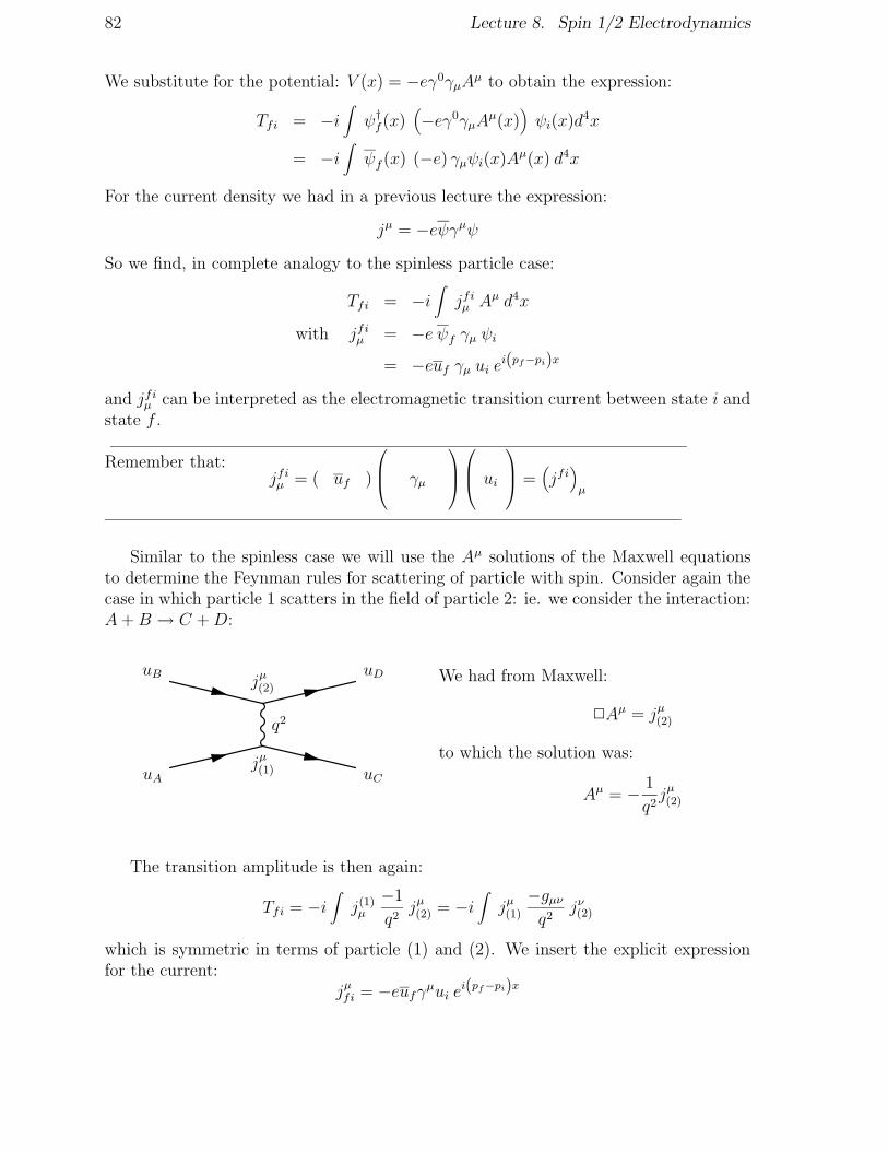
82 Lecture 8. Spin 1/2 Electrodynamics
We substitute for the potential: V (x) = −eγ0γµAµ to obtain the expression:
Tfi = −i∫
ψ†f (x)(
−eγ0γµAµ(x))
ψi(x)d4x
= −i∫
ψf (x) (−e) γµψi(x)Aµ(x) d4x
For the current density we had in a previous lecture the expression:
jµ = −eψγµψ
So we find, in complete analogy to the spinless particle case:
Tfi = −i∫
jfiµ Aµ d4x
with jfiµ = −e ψf γµ ψi= −euf γµ ui ei(pf−pi)x
and jfiµ can be interpreted as the electromagnetic transition current between state i andstate f .
Remember that:jfiµ = ( uf )
γµ
ui
=
(
jfi)
µ
Similar to the spinless case we will use the Aµ solutions of the Maxwell equationsto determine the Feynman rules for scattering of particle with spin. Consider again thecase in which particle 1 scatters in the field of particle 2: ie. we consider the interaction:A+B → C +D:
q2
uA
uB
uC
uD
jµ(1)
jµ(2)We had from Maxwell:
2Aµ = jµ(2)
to which the solution was:
Aµ = − 1
q2jµ(2)
The transition amplitude is then again:
Tfi = −i∫
j(1)µ
−1q2
jµ(2) = −i∫
jµ(1)−gµνq2
jν(2)
which is symmetric in terms of particle (1) and (2). We insert the explicit expressionfor the current:
jµfi = −eufγµui ei(pf−pi)x

8.2. Electron - Muon Scattering 83
to obtain:
Tfi = −i∫
−euCγµuA ei(pC−pA)x ·−gµνq2
· −euDγνuB ei(pD−pB)x
So that we arrive at the “Feynman Rules”:
Tfi = −i (2π)4 δ4 (pD + pC − pB − pA) · M
−iM = ie (uCγµuA)
︸ ︷︷ ︸
vertex
· −igµνq2
︸ ︷︷ ︸
propagator
· ie (uDγνuB)︸ ︷︷ ︸
vertex
without spin: with spin:
1 1ie (pf + pi)
µ ui ufieγµ
Figure 8.1: Vertex factors for left: spinless particles, right: spin 1/2 particles.
8.2 Electron - Muon Scattering
We proceed to use the Feynman rules to calculate the cross section of the process:e−µ− → e−µ−. We want to calculate the unpolarized cross section:
• The incoming particles are not polarized. This implies that we average over spinsin the initial state.
• The polarization of the final state particles is not measured. This implies that wesum over the spins in the final state.
The spin summation and averaging means that we replace the matrix element by:
|M|2 → |M|2 = 1
(2sA + 1) (2sB + 1)
∑
Spin
|M|2
where 2sA + 1 is the number of spin states of particle A and 2sB + 1 for particle B. Sothe product (2sA + 1) (2sB + 1) is the number of spin states in the initial state.
−iM = −igµνq2
e− : uA
µ− : uB
e− : uC
µ− : uD
ieuCγµuA
ieuDγνuB
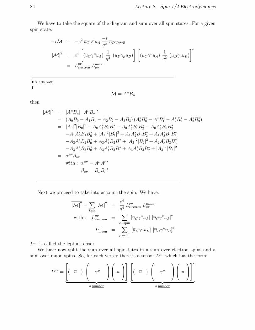
84 Lecture 8. Spin 1/2 Electrodynamics
We have to take the square of the diagram and sum over all spin states. For a givenspin state:
−iM = −e2 uCγµuA−iq2
uDγµuB
|M|2 = e4[
(uCγµuA)
1
q2(uDγµuB)
] [
(uCγνuA)
1
q2(uDγνuB)
]∗
= Lµνelectron Lmuonµν
Intermezzo:If
M = AµBµ
then
|M|2 = [AµBµ] [AνBν ]
∗
= (A0B0 − A1B1 − A2B2 − A3B3) (A∗0B
∗0 − A∗1B
∗1 − A∗2B
∗2 − A∗3B
∗3)
= |A0|2|B0|2 − A0A∗1B0B
∗1 − A0A
∗2B0B
∗2 − A0A
∗3B0B
∗3
−A1A∗0B1B
∗0 + |A1|2|B1|2 + A1A
∗2B1B
∗2 + A1A
∗3B1B
∗3
−A2A∗0B2B
∗0 + A2A
∗1B2B
∗1 + |A2|2|B2|2 + A2A
∗3B2B
∗3
−A3A∗0B3B
∗0 + A3A
∗1B3B
∗1 + A3A
∗2B3B
∗2 + |A3|2|B3|2
= αµνβµν
with : αµν = AµAν∗
βµν = BµBν∗
Next we proceed to take into account the spin. We have:
|M|2 =∑
Spin
|M|2 =e4
q4Lµνelectron L
muonµν
with : Lµνelectron =∑
e−spin[uCγ
µuA] [uCγνuA]
∗
Lµνmuon =∑
µ−spin[uDγ
µuB] [uDγνuB]
∗
Lµν is called the lepton tensor.We have now split the sum over all spinstates in a sum over electron spins and a
sum over muon spins. So, for each vertex there is a tensor Lµν which has the form:
Lµν =
( u )
γµ
u
︸ ︷︷ ︸
a number
( u )
γν
u
∗
︸ ︷︷ ︸
a number
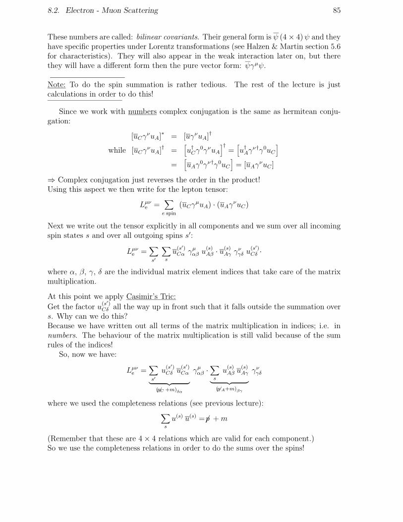
8.2. Electron - Muon Scattering 85
These numbers are called: bilinear covariants. Their general form is ψ (4× 4)ψ and theyhave specific properties under Lorentz transformations (see Halzen & Martin section 5.6for characteristics). They will also appear in the weak interaction later on, but therethey will have a different form then the pure vector form: ψγµψ.
Note: To do the spin summation is rather tedious. The rest of the lecture is justcalculations in order to do this!
Since we work with numbers complex conjugation is the same as hermitean conju-gation:
[uCγνuA]
∗ = [uγνuA]†
while [uCγνuA]
† =[
u†Cγ0γνuA
]†=[
u†Aγν†γ0uC
]
=[
uAγ0γν†γ0uC
]
= [uAγνuC ]
⇒ Complex conjugation just reverses the order in the product!Using this aspect we then write for the lepton tensor:
Lµνe =∑
e spin
(uCγµuA) · (uAγνuC)
Next we write out the tensor explicitly in all components and we sum over all incomingspin states s and over all outgoing spins s′:
Lµνe =∑
s′
∑
s
u(s′)Cα γ
µαβ u
(s)Aβ · u
(s)Aγ γ
νγδ u
(s′)Cδ ·
where α, β, γ, δ are the individual matrix element indices that take care of the matrixmultiplication.
At this point we apply Casimir’s Tric:
Get the factor u(s′)Cδ all the way up in front such that it falls outside the summation over
s. Why can we do this?Because we have written out all terms of the matrix multiplication in indices; i.e. innumbers. The behaviour of the matrix multiplication is still valid because of the sumrules of the indices!
So, now we have:
Lµνe =∑
s′
u(s′)Cδ u
(s′)Cα
︸ ︷︷ ︸
(6pC +m)δα
γµαβ ·∑
s
u(s)Aβ u
(s)Aγ
︸ ︷︷ ︸
(6p A+m)βγ
γνγδ
where we used the completeness relations (see previous lecture):∑
s
u(s) u(s) =6p +m
(Remember that these are 4× 4 relations which are valid for each component.)So we use the completeness relations in order to do the sums over the spins!
86 Lecture 8. Spin 1/2 Electrodynamics
The result is:Lµνe = (6p C +m)δα γ
µαβ (6p A +m)βγ γ
νγδ
Here is the next trick: look at the indices α, β, γ, δ; they are components of 4×4matrices. Perform the sum over the indices α, β, γ and say that the result is: A. Thenwe find that Lµνe ∝ Aδδ and we have to do the remaining sum over δ, which means thatwe take the trace of the matrix. In other words, the fact that we sum over all indicesmeans:
Lµνe = Tr [( 6p C +m) γµ (6p A +m) γν ]
Where are we at this point?We look at the reaction e−µ− → e−µ− and we have:
|M|2 =1
(2sA + 1) (2sB + 1)
∑
Spin
|M|2
=1
(2sA + 1) (2sB + 1)
e4
q4Lµνe Lmµν
with : Lµνe = Tr [(6p C +m) γµ (6p A +m) γν ]
Lmµν = Tr [(6p D +m) γµ (6p B +m) γν ]
In order to evaluate these expressions we make use of trace identities.
Intermezzo: Trace theorems
• In general:
– Tr (A+B) = Tr(A) + Tr(B)
– Tr (ABC) = Tr (CAB) = Tr (BCA)
• For γ-matrices: from the definition: γµγν + γνγµ = 2gµν it follows:
– Tr (odd number of γµ’s = 0). ⇒ only 0 on the diagonal.
– Tr (γµγν) = 4 gµν . ⇒ note that this is a matrix of traces!
– Tr (6a 6b ) = 4 a · b– Tr (6a 6b 6c 6d ) = 4 [ (a · b) (c · d)− (a · c) (b · d) + (a · d) (b · c) ]
We are calculating:
Lµνe = Tr [(6p C +m) γµ (6p A +m) γν ] .....write it out.....
= Tr [ 6p Cγµ 6p Aγ
ν ]︸ ︷︷ ︸
case 2
+Tr [mγµmγν ]︸ ︷︷ ︸
case 1
+Tr [6p Cγµmγν ]
︸ ︷︷ ︸
3γ′s⇒0
+Tr [mγµ 6p Aγν ]
︸ ︷︷ ︸
3γ′s⇒0

8.2. Electron - Muon Scattering 87
Case 1: Tr [mγµmγν ] = m2Tr [γµγν ] = 4m2gµν
Case 2: Tr [ 6p Cγµ 6p Aγ
ν ] =?Use the rule for Tr (6a 6b 6c 6d ) with a = pC and c = pA, but what are b and d?⇒ b must be chosen such that γα · b = γµ. ⇒ b = gαµ.⇒ d must be chosen such that γβ · d = γν . ⇒ d = gβν .Therefore:
Tr [6p Cγµ 6p Aγ
ν ]
= 4[(
pCαgαµ) (
pAβgβν)
− (pαCpAα)(
gαµgβνgµν)
+ (pCαgαν)
(
pAβgβµ)]
= 4 [pµCpνA + pνCp
µA − (pC · pA) gµν ]
Finally we find for the tensors:
Lµνe = 4[
pµCpνA + pνCp
µA −
(
pC · pA −m2e
)
gµν]
Lmµν = 4[
pDµpBν + pDνpBµ −(
pD · pB −m2m
)
gµν]
To recapitulate, the matrix element for e−µ− → e−µ−:
|M|2 = 1
(2sA + 1) (2sB + 1)· e
4
q4· Lµνe Lmµν
and will just fill in the results of the tensors we just calculated:
Lµνe Lmµν = 4[
pµCpνA + pνCp
µA −
(
pC · pA −m2e
)
gµν]
· 4[
pDµpBν + pDνpBµ −(
pD · pB −m2m
)
gµν]
= 16 ·(pC · pD) (pA · pB) + (pC · pB) (pA · pD)− (pC · pA) (pD · pB) + (pC · pA)m2
m
(pC · pB) (pA · pD) + (pC · pD) (pA · pB)− (pC · pA) (pD · pB) + (pC · pA)m2m
− (pC · pA) (pD · pB)− (pC · pA) (pD · pB) + (pC · pA) (pD · pB) · 4− (pC · pA)m2m · 4
+m2e (pD · pB) +m2
e (pD · pB)− 4m2e (pD · pB) + 4m2
em2m
= 32 ·[
(pA · pB) (pC · pD) + (pA · pD) (pC · pB)−m2e (pD · pB)−m2
m (pA · pC) + 2m2em
2m
]
We then obtain:
|M|2 =1
2· 12· e
4
q4· Lµνe Lmµν
= 8e4
q4
[
(pC · pD) (pA · pB) + (pC · pB) (pA · pD)−m2e (pD · pB)−m2
m (pA · pC) + 2m2em
2m
]
Let us consider the ultrarelativistic limit; ie. we ignore the masses of the particleswith respect to their momentum. Also we use the Mandelstam variables:
s ≡ (pA + pB)2 = p2A + p2B + 2 (pA · pB) ' 2 (pA · pB)
t ≡ (pD − pB)2 ≡ q2 ' −2 (pD · pB)
u ≡ (pA − pD)2 ' −2 (pA · pD)
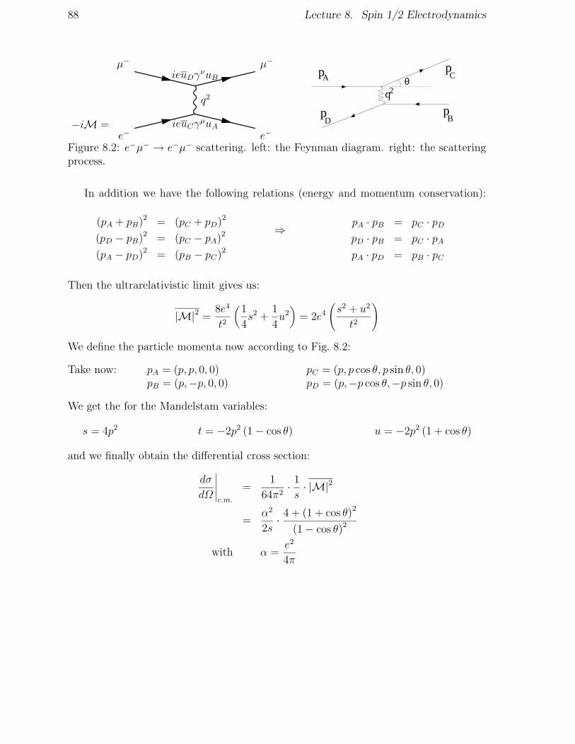
88 Lecture 8. Spin 1/2 Electrodynamics
−iM =
q2
e−
µ−
e−
µ−
ieuCγµuA
ieuDγνuB
pC
pB
Ap
pD
q2θ
Figure 8.2: e−µ− → e−µ− scattering. left: the Feynman diagram. right: the scatteringprocess.
In addition we have the following relations (energy and momentum conservation):
(pA + pB)2 = (pC + pD)
2
(pD − pB)2 = (pC − pA)
2
(pA − pD)2 = (pB − pC)
2
⇒ pA · pB = pC · pDpD · pB = pC · pApA · pD = pB · pC
Then the ultrarelativistic limit gives us:
|M|2 = 8e4
t2
(1
4s2 +
1
4u2)
= 2e4(
s2 + u2
t2
)
We define the particle momenta now according to Fig. 8.2:
Take now: pA = (p, p, 0, 0) pC = (p, p cos θ, p sin θ, 0)pB = (p,−p, 0, 0) pD = (p,−p cos θ,−p sin θ, 0)
We get the for the Mandelstam variables:
s = 4p2 t = −2p2 (1− cos θ) u = −2p2 (1 + cos θ)
and we finally obtain the differential cross section:
dσ
dΩ
∣∣∣∣∣c.m.
=1
64π2· 1s· |M|2
=α2
2s· 4 + (1 + cos θ)2
(1− cos θ)2
with α =e2
4π

8.3. Crossing: the process e+e− → µ+µ− 89
8.3 Crossing: the process e+e− → µ+µ−
We will use the “crossing” principle to obtain |M|2(e+e−→µ+µ−) from the result of |M|2(e−µ−→e−µ−)
B
An anti−particle is a particle wherep is replaced by −p. The diagram in terms of particles is:
e e
µ µ
− −
− −−
e
e
µ
µ
µ
e
e
µ
− −
+ +
−e µe µ+ +−µ−e−µ−e−
p
p’ p’
p’ p’
Ap
B
pC
Dp
A
B
C
D
p’ p’
−p’−p’
A
B
C
D
P
P
P
P
Replace:
A
B
C
D
P’
−P’
−P’
P’
A
D
C
Figure 8.3: The principle of crossing. Use the anti-particle interpretation of a particlewith the 4-momentum reversed in order to related the Matrix element of the “crossed”reaction to the original one.
So we replace in the previously obtained result:
s = 2 (pA · pB) → −2 (p′A · p′D) = u′
t = −2 (pA · pC) → 2 (p′A · p′B) = s′
u = −2 (pA · pD) → −2 (p′A · p′C) = t′
So that we have:
|M|2e−µ−→e−µ− = 2e4s2 + u2
t2
|M|2e−e+→µ−µ+ = 2e4u′2 + t′2
s′2
“t-channel”: q2 = t
“s-channel”:q2 = s
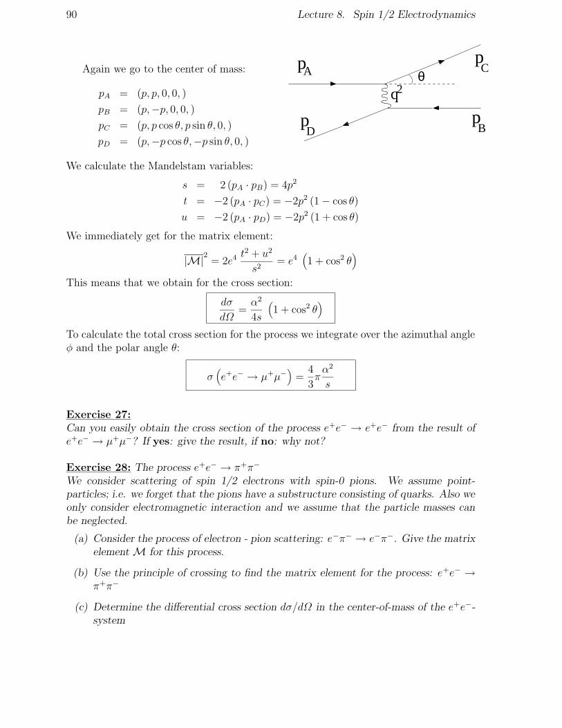
90 Lecture 8. Spin 1/2 Electrodynamics
Again we go to the center of mass:
pA = (p, p, 0, 0, )
pB = (p,−p, 0, 0, )pC = (p, p cos θ, p sin θ, 0, )
pD = (p,−p cos θ,−p sin θ, 0, )
pC
pB
Ap
pD
q2θ
We calculate the Mandelstam variables:
s = 2 (pA · pB) = 4p2
t = −2 (pA · pC) = −2p2 (1− cos θ)
u = −2 (pA · pD) = −2p2 (1 + cos θ)
We immediately get for the matrix element:
|M|2 = 2e4t2 + u2
s2= e4
(
1 + cos2 θ)
This means that we obtain for the cross section:
dσ
dΩ=α2
4s
(
1 + cos2 θ)
To calculate the total cross section for the process we integrate over the azimuthal angleφ and the polar angle θ:
σ(
e+e− → µ+µ−)
=4
3πα2
s
Exercise 27:Can you easily obtain the cross section of the process e+e− → e+e− from the result ofe+e− → µ+µ−? If yes: give the result, if no: why not?
Exercise 28: The process e+e− → π+π−
We consider scattering of spin 1/2 electrons with spin-0 pions. We assume point-particles; i.e. we forget that the pions have a substructure consisting of quarks. Also weonly consider electromagnetic interaction and we assume that the particle masses canbe neglected.
(a) Consider the process of electron - pion scattering: e−π− → e−π−. Give the matrixelement M for this process.
(b) Use the principle of crossing to find the matrix element for the process: e+e− →π+π−
(c) Determine the differential cross section dσ/dΩ in the center-of-mass of the e+e−-system

Lecture 9
The Weak Interaction
In 1896 Henri Becquerel observed that Uranium affected photographic plates. He wasstudying the effect of fluorescence, which he thought was caused by the X-rays thatwere discovered by Wilhelm Rontgen. To test his hypothesis he wanted to observe thatthis fluorescence radiation also affected photographic plates. He discovered by accidentthat the Uranium salt he used also affected the photographic plate when they were notexposed to sunlight. Thus he discovered natural radioactivity.
We know now that the weak interaction in nature is based on the decay: n→ p+ e− + νeand has a lifetime of τ = 886s.
np+
e−
νe
Compare the lifetimes of the following decays:
weak : π− → µ−νµ τ = 2.6 · 10−8 secµ− → e−νeνµ τ = 2.2 · 10−6 sec
with : e.m. : π0 → γγ τ = 8.4 · 10−17 secstrong : ρ→ ππ τ = 4.4 · 10−23 sec (Γ = 150 MeV)
and realise that the lifetime of a process is inversely proportional to the strength of theinteraction. Note in addition that:
1. All fermions “feel” the weak interaction. However, when present the electromag-netic and strong interactions dominate.
2. Neutrino’s feel only the weak interaction. This is the reason why they are so hardto detect.
91

92 Lecture 9. The Weak Interaction
9.1 The 4-point interaction
Based on the model of electromagnetic interactions Fermi inventd in 1932 the so-called4-point interaction model, introducing the Fermi constant as the strength of the inter-action: GF ≈ 1.166 · 10−5Gev−2
νe
n
e−
p+ The “Feynman diagram” of the 4-point in-teraction “neutrino scattering on a neutron”has the following matrix element:
M = GF (upγµun) (ueγµuν)
This is to be compared to the electromagnetic diagram for electron proton scattering:
q2
e−
p+
e−
p+Here the matrix element was:
M =4πα
q2(upγ
µup) (ueγµue)
1. e2 = 4πα is replaced by GF
2. 1/q2 is removed
We take note of the following facts of the weak interaction:
1. The hadronic current jhµ has ∆Q = 1, the leptonic current has ∆Q = −1. Werefer to this as: charged currents, since there is a net charge transferred from thehadron current to the lepton current. We will see later that neutral weak currentsturn out to exist as well.
2. There is a coupling constant GF , which now plays a similar role as α in QED.
3. There is no propagator; ie. a “4-point interaction”.
4. The currents have what is called a “vector character” similar as in QED. Thismeans that the currents are of the form ψγµψ.
The vector character of the interaction was in fact just a guess that turned out successfulto describe many aspects of β-decay. There was no reason for this choice apart fromsimilarity of QED. In QED the reason that the interaction has a vector behaviour is thefact that the force mediator, the foton, is a spin-1, or vector particle.
In the most general case the matrix element of the 4-point interaction can be writtenas:
M = GF
(
ψp (4× 4) ψn) (
ψe (4× 4) ψν)
where (4× 4) are combinations of γ-matrices. Lorentz invariance of the interaction putsrestrictions on the form of the bilinear covariants of any possible interaction.

9.1. The 4-point interaction 93
For any possible theory (or “force”) the bilinear covariants can be of the followingtype:
current # components # γ-matrices spin
Scalar ψψ 1 0 0Vector ψγµψ 4 1 1Tensor ψσµνψ 6 2 2Axial vector ψγ5γµψ 4 3 1Pseudo scalar ψγ5ψ 1 4 0
Table 9.1: Possible forms of the bilinear covariants. σµν ≡ i2(γµγν − γνγµ). Note that
the total number of components is 16.
In the most general case the 4-point weak interaction can be written as:
M = GF
S,P,V,A,T∑
i,j
Cij (up Oi un) (ue Oj uν)
where Oi, Oj are operators of the form S, V , T , A, P .It can be shown with Dirac theory (see eg. Perkins: “Introduction to High EnergyPhysics”, 3rd edition, appendix D) that:S, P , T interactions in n→ peνe imply: helicity e = helicity νe,V , A, interactions in n→ peνe imply: helicity e = -helicity νe.
In 1958 Goldhaber et. al. measured experimentally that the weak interaction is ofthe type: V , A, (ie. it is not S, P , T ). See Perkins ed 3, §7.5 for a full description ofthe experiment. The basic idea is the following.Consider the electron capture reaction: 152Eu + e− →152 Sm∗(J = 1) + ν
1/2
+ e− + =+1/2νλ
+ e− + λ =ν −1/2
Eu152 + e− 152Sm* + ν
B)
A)1/21/2 1
11/2
By studying the consecutive decay 152Sm∗ →152 Sm + γ it was observed that onlycase B actually occurred. In other words: neutrino’s have helicity -1/2. From this itwas concluded that in the weak interaction only the V , A currents are involved and notS, P , T !
Let us take a look at the partity operator which inverts space: ie. t → t ; ~r → −~r.The parity Lorentz transformation is:
Λµν =
1−1
−1−1

94 Lecture 9. The Weak Interaction
Which is the “Dirac” operator that gives: ψ′(x′) = Sψ(x) (and also S−1γµS = Λµνγν)?
Assume that the wave function ψ (~r, t) is a solution of the Dirac equation:
(
γ0∂
∂t+ γk
∂
∂xk−m
)
ψ (~r, t) = 0
then, after a parity transformation (note that: γ0 → γ0 and γk → −γk) we find:
(
γ0∂
∂t− γk
∂
∂xk−m
)
ψ (−~r, t) = 0
So, ψ (−~r, t) is not a solution of the Dirac equation due to the additional - sign! Letus multiply the Dirac equation of the parity transformed spinor from the left by γ0, tofind:
γ0
(
γ0∂
∂t− γk
∂
∂xk−m
)
ψ (−~r, t) = 0
⇒(
γ0∂
∂tγ0 + γk
∂
∂xkγ0 −mγ0
)
ψ (−~r, t) = 0
⇒(
γ0∂
∂t+ γk
∂
∂xk−m
)
γ0ψ (−~r, t) = 0
We conclude that if ψ (~r, t) is a solution of the Dirac equation, then γ0ψ (−~r, t) is alsoa solution (in the mirror world).In other words: under the parity operation (S = γ0): ψ (~r, t)→ γ0ψ (−~r, t).
What does this imply for the currents in the interactions? Under the Parity operatorwe get:
S : ψψ → ψγ0γ0ψ = ψψ Scalar
P : ψγ5ψ → ψγ0γ5γ0ψ = −ψγ5ψ Pseudo Scalar
V : ψγµψ → ψγ0γµγ0ψ =
ψγ0ψ−ψγkψ Vector
A : ψγ5γµψ → ψγ5γ0γµγ0ψ =
−ψγ0ψψγkψ
Axial Vector.
We had concluded earlier that the weak matrix element in neutron decay is of theform:
M = GF
V,A∑
i,j
Cij (upOiup) (ueOjuν)
But: if there is a contribution from vector as well as from axial vector then we musthave parity violation!

9.2. The V − A interaction 95
9.2 The V − A interaction
It turns out that the only change that is needed in the pure vector coupling of Fermi is:
(ue γµ uν)→
(
ue γµ 1
2
(
1− γ5)
uν
)
This is the famous V −A interaction where the vector coupling and the axial vector cou-pling are equally strong present. The consequence is that there is maximal violationof parity in the weak interaction.
For neutron decays there is a complication to test the V − A structure since theneutron and the proton are not point particles. The observed matrix element for neutrondecays is:
M =GF√2
(
upγµ(
CV − CAγ5)
un) (
ueγµ(
1− γ5)
uν)
It has the follwing values for the vector andaxial vector couplings:CV = 1.000± 0.003, CA = 1.260± 0.002However, the fundamental weak interactionbetween the quarks and the leptons are pureV − A.
e
n p+
ν
9.3 The Propagator of the weak interaction
The Fermi theory has a 4-point interaction: there is no propagator involved to transmitthe interaction from the lepton current to the hadron current. However, we know nowthat forces are carried by bosons:
• the electromagnetic interaction is carried by the massless photon which gives riseto a → 1
q2propagator
• the weak interaction is carried by the massive W , Z bosons, for which we havethe propagators: 1
M2W−q2 and 1
M2Z−q2 .
Let us consider an interaction at low energy; ie. the case that M 2W >> q2. In that case
the propagator reduces to 1M2
W
.
gW
g
strength: ∼ GF√2
∼ g2
8M2W
We interpret the coupling constant g of the weak interaction exactly like e in QED.

96 Lecture 9. The Weak Interaction
How “weak” is the weak interaction?In QED we have: α = e2
4π= 1
137
In the weak interaction it turns out: αw = g2
4π= 1
29
The interaction is weak because the mass MW is high! The intrinsic coupling constantis not small in comparison to QED. As a consequence it will turn out that at highenergies: q2 ∼M2
W the weak interaction is comparable in strength to the electromagneticinteraction.
9.4 Muon Decay
Similar to the process e+e− → µ+µ− in QED, the muon decay process µ− → e−νeνµ isthe standard example of a weak interaction process.
µ
ννe
eµ−(p)
(k’)
(k)
−(p’)
Wµ(p)−
νµ (k)
e−(p’)
νe(−k’)
Figure 9.1: Muon decay: left: Labelling of the momenta, right: Feynman diagram. Notethat for the spinor of the outgoing antiparticle we use: uνe(−k′) = vνe(k
′).
Using the Feynman rules we can write for the matrix element:
M =g√2
u(k)
︸ ︷︷ ︸
outgoing µν
γµ1
2
(
1− γ5)
u(p)︸ ︷︷ ︸
incoming µ
1
M2W
︸ ︷︷ ︸
propagator
g√2
u(p′)︸ ︷︷ ︸
outgoing e
γµ1
2
(
1− γ5)
v(k′)︸ ︷︷ ︸
outgoing νe
Next we square the matrix element and sum over the spin states, exactly similarto the case of e+e− → µ+µ−. Then we use again the tric of Casimir as well as thecompleteness relations to convert the sum over spins into a trace. The result is:
|M| = 1
2
∑
Spin
|M|2 = 1
2
(
g2
8M2W
)2
· Tr
γµ(
1− γ5)
(6p ′ +me) γν(
1− γ5)
6k ′
· Tr
γµ(
1− γ5)
6k γν(
1− γ5)
(6p +mµ)
Now we use some more trace theorems (see below) and also GF√2= g2
8M2W
to find the result:
|M| = 64G2F (k · p′) (k′ · p)
Intermezzo: Trace theorems used (see also Halzen & Martin p 261):
Tr (γµ 6a γν 6b ) · Tr (γµ 6c γν 6d ) = 32 [(a · c) (b · d) + (a · d) (b · c)]

9.4. Muon Decay 97
Tr(
γµ 6a γνγ5 6b)
· Tr(
γµ 6c γνγ5 6d)
= 32 [(a · c) (b · d)− (a · d) (b · c)]Tr(
γµ(
1− γ5)
6a γν(
1− γ5)
6b)
· Tr(
γµ(
1− γ5)
6c γν(
1− γ5)
6d)
= 256 (a · c) (b · d)
The decay width we can find by applying Fermi’s golden rule:
dΓ =1
2E|M| dQ
where : dQ =d3p′
(2π)3 2E· d3k
(2π)3 2ω· d3k′
(2π)3 2ω′· (2π)4 δ4 (p− p′ − k′ − k)
with :E = muon energy
E ′ = electron energy
ω′ = electron neutrino energy
ω = muon neutrino energy
First we evaluate the expression for the matrix element. We have the relation(p = (mµ, 0, 0, 0)):
p = p′ + k + k′ so : (k + p′) = (p− k′)
We can also see the following relations to hold:
(k + p′)2
= k2︸︷︷︸
=0
+ p′2︸︷︷︸
m2e≈0
+2 (k · p′)
(p− k′)2
= p2︸︷︷︸
m2µ≡m2
+ k′2︸︷︷︸
=0
−2 (p · k′)︸ ︷︷ ︸
mω′
Therefor we have the relation: 2 (k · p′) = m2−2mω′, which we use to rewrite the matrixelement as:
|M| = 64G2F (k · p′) (k′ · p) = 32G2
F
(
m2 − 2mω′)
mω′
We had the expression for the decay time:
dΓ =1
2E|M| dQ =
16G2F
m
(
(m2 − 2mω′)
mω′ dQ
(E is replaced by m since the decaying muon is in rest). For the total decay width wemust integrate over the phase space:
Γ =∫ 1
2E|M| dQ =
16G2F
m
∫ (
(m2 − 2mω′)
mω′ dQ

98 Lecture 9. The Weak Interaction
We note that the integrand only depends on the neutrino energy ω ′. So, let us firstperform the integral in dQ over the other energies and momenta:
∫
otherdQ =
1
8 (2π)5
∫
δ (m− E ′ − ω′ − ω) δ3(
~p′ + ~k′ + ~k) d3~p′
E ′d3~k′
ω′d3~k
ω
=1
8 (2π)5
∫
δ (m− E ′ − ω′ − ω)d3~p′ d3~k′
E ′ω′ω
since the δ-function gives 1 for the integral over ~k.We also have the relation:
ω = |k| = |~p′ + ~k′| =√E ′2 + ω′2 + 2E ′ω′ cos θ
where θ is the angle between the electron and the electron neutrino. We choose thez-axis along ~k′, the direction of the electron neutrino. From the equation for ω wederive:
dω =−2E ′ω′ sin θ
2√E ′2 + ω′2 + 2E ′ω′ cos θ
︸ ︷︷ ︸
ω
dθ ⇔ dθ =−ω dωE ′ω′ sin θ
Next we integrate over d3~p′ = E ′2 sin θ dE ′ dθ dφ with dθ as above:
dQ =1
8 (2π)5
∫
δ (m− E ′ − ω′ − ω)E ′2 sin θ
E ′dE ′ dθ dφ
d3~k′
ω′1
ω
=1
8 (2π)52π
∫
δ (m− E ′ − ω′ − ω) dE ′ dωd3~k′
ω′2
(using the relation: E ′ sin θ dθ = − ωω′dω).
Since we integrate over ω, the δ-function will cancel:
dQ =1
8 (2π)4
∫
dE ′d3~k′
ω′2
such that the full expression for Γ becomes:
Γ =2G2
F
(2π)4
∫ (
m2 − 2mω′)
ω′ dE ′d3~k′
ω′2
Next we do the integral over k′ as far as possible with:
∫
d3~k′ =∫
ω′2 sin θ′ dω′ dθ′ dφ′ = 4π∫
ω′2 dω
so that we get:
Γ =G2Fm
(2π)3
∫
(m− 2ω′) ω′ dω′ dE ′
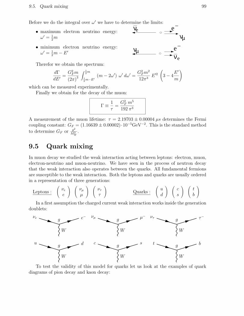
9.5. Quark mixing 99
Before we do the integral over ω′ we have to determine the limits:
• maximum electron neutrino energy:ω′ = 1
2m
• minimum electron neutrino energy:ω′ = 1
2m− E ′
e
ν e−
e−
ν
νν
e
µ
µ
Therefor we obtain the spectrum:
dΓ
dE ′=G2Fm
(2π)3
∫ 12m
12m−E′
(m− 2ω′) ω′ dω′ =G2Fm
2
12π3E ′2
(
3− 4E ′
m
)
which can be measured experimentally.Finally we obtain for the decay of the muon:
Γ ≡ 1
τ=G2F m
5
192 π3
A measurement of the muon lifetime: τ = 2.19703 ± 0.00004 µs determines the Fermicoupling constant: GF = (1.16639± 0.00002) ·10−5GeV−2. This is the standard method
to determine GF or g2
M2W
.
9.5 Quark mixing
In muon decay we studied the weak interaction acting between leptons: electron, muon,electron-neutrino and muon-neutrino. We have seen in the process of neutron decaythat the weak interaction also operates between the quarks. All fundamental fermionsare susceptible to the weak interaction. Both the leptons and quarks are usually orderedin a representation of three generations:
Leptons :
(
νee
) (
νµµ
) (
νττ
)
Quarks :
(
ud
) (
cs
) (
tb
)
In a first assumption the charged current weak interaction works inside the generationdoublets:
W
νe e−g
W
νµ µ−g
W
ντ τ−g
W
u dg
W
c sg
W
t bg
To test the validity of this model for quarks let us look at the examples of quarkdiagrams of pion decay and kaon decay:

100 Lecture 9. The Weak Interaction
1. pion decay
π− → µ−νµΓπ− ∝ g4
M2W
∝ G2F
Wπ−
u
d
g g µ−
νµ
2. kaon decay
K− → µ−νµThis decay does occur!
??−u
g µ−
νµWs
K
9.5.1 Cabibbo - GIM mechanism
We have to modify the model by the replacements:
d → d′ = d cos θc + s sin θc
s → s′ = −d sin θc + s cos θc
or, in matrix representation:
(
d′
s′
)
=
(
cos θc sin θc− sin θc cos θc
)(
ds
)
where θc is the Cabibbo mixing angle.
In terms of the diagrams the replacement implies:
W
u dg
⇒W
u d′g
=W
u dg cos θc
+W
u sg sin θc
Both the u, d coupling and the u, s coupling exist. In this case the diagrams of piondecay and kaon decay are modified:
1. Pion decay
π− → µ−νµΓπ− ∝ G2
F cos2 θcπ−
u
d
g µ−
νµW
θgcos
2. Kaon decay
K− → µ−νµΓK− ∝ G2
F sin2 θc s
−u
g µ−
νµW
θK
gsin
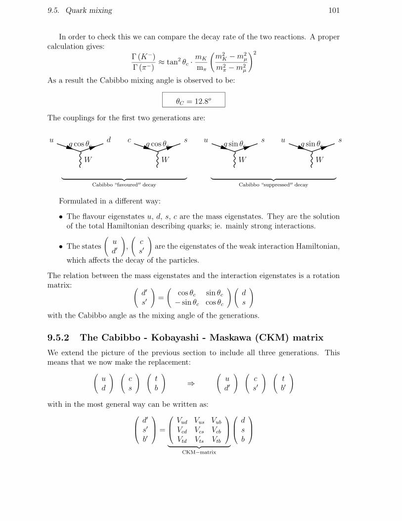
9.5. Quark mixing 101
In order to check this we can compare the decay rate of the two reactions. A propercalculation gives:
Γ (K−)
Γ (π−)≈ tan2 θc ·
mK
mπ
(
m2K −m2
µ
m2π −m2
µ
)2
As a result the Cabibbo mixing angle is observed to be:
θC = 12.8o
The couplings for the first two generations are:
W
u dg cos θc
W
c sg cos θc
W
u sg sin θc
W
u sg sin θc
︸ ︷︷ ︸
Cabibbo “favoured′′ decay
︸ ︷︷ ︸
Cabibbo “suppressed′′ decay
Formulated in a different way:
• The flavour eigenstates u, d, s, c are the mass eigenstates. They are the solutionof the total Hamiltonian describing quarks; ie. mainly strong interactions.
• The states
(
ud′
)
,
(
cs′
)
are the eigenstates of the weak interaction Hamiltonian,
which affects the decay of the particles.
The relation between the mass eigenstates and the interaction eigenstates is a rotationmatrix: (
d′
s′
)
=
(
cos θc sin θc− sin θc cos θc
)(
ds
)
with the Cabibbo angle as the mixing angle of the generations.
9.5.2 The Cabibbo - Kobayashi - Maskawa (CKM) matrix
We extend the picture of the previous section to include all three generations. Thismeans that we now make the replacement:
(
ud
) (
cs
) (
tb
)
⇒(
ud′
) (
cs′
) (
tb′
)
with in the most general way can be written as:
d′
s′
b′
=
Vud Vus VubVcd Vcs VcbVtd Vts Vtb
︸ ︷︷ ︸
CKM−matrix
dsb
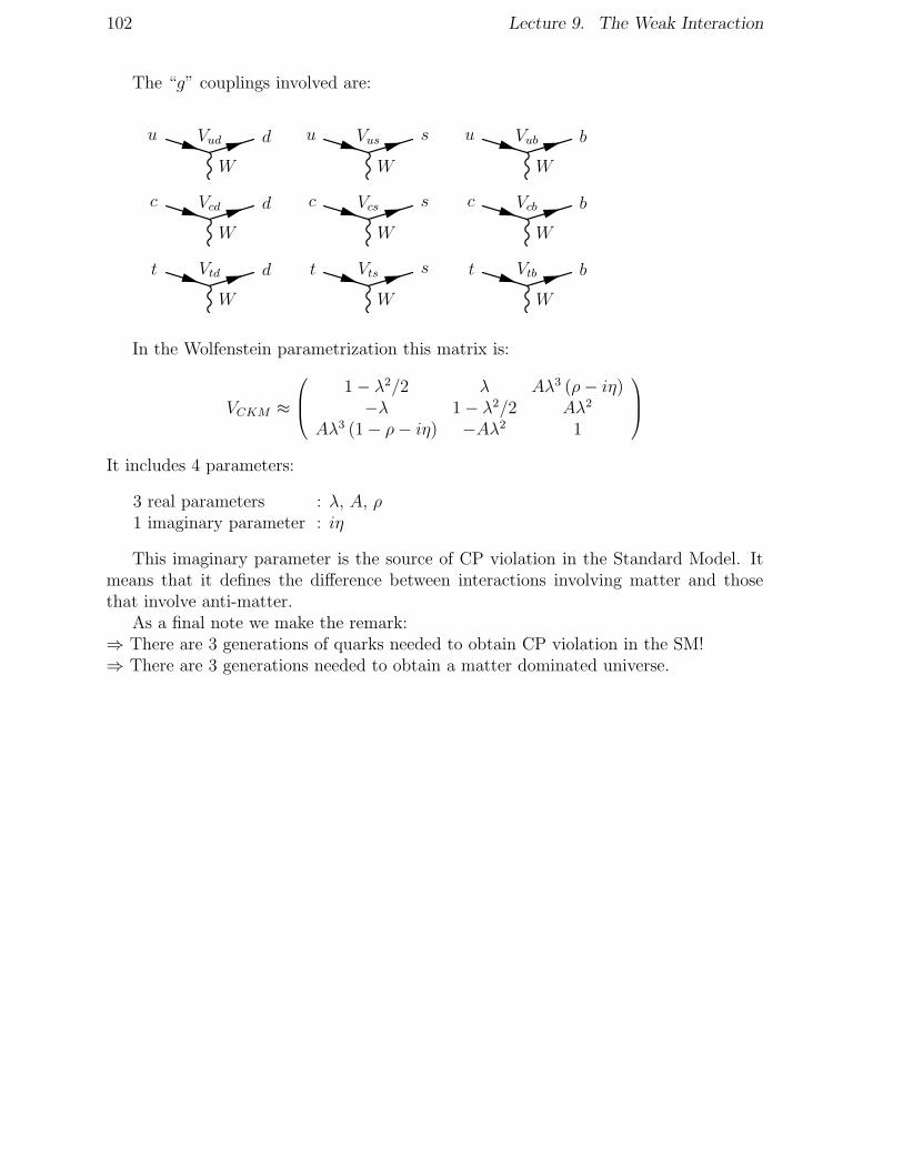
102 Lecture 9. The Weak Interaction
The “g” couplings involved are:
W
u dVud
W
u sVus
W
u bVub
W
c dVcd
W
c sVcs
W
c bVcb
W
t dVtd
W
t sVts
W
t bVtb
In the Wolfenstein parametrization this matrix is:
VCKM ≈
1− λ2/2 λ Aλ3 (ρ− iη)−λ 1− λ2/2 Aλ2
Aλ3 (1− ρ− iη) −Aλ2 1
It includes 4 parameters:
3 real parameters : λ, A, ρ1 imaginary parameter : iη
This imaginary parameter is the source of CP violation in the Standard Model. Itmeans that it defines the difference between interactions involving matter and thosethat involve anti-matter.
As a final note we make the remark:⇒ There are 3 generations of quarks needed to obtain CP violation in the SM!⇒ There are 3 generations needed to obtain a matter dominated universe.
9.5. Quark mixing 103
Exercise 29: Pion DecayUsually at this point the student is asked to calculate pion decay, which requires againquite some calculations. The ambitious student is encourage to try and do it (using somehelp from the literature). However, the exercise below requires little or no calculationbut instead insight in the formalism.
(a) Draw the Feynman diagram for the decay of a pion to a muon and an anti-neutrino:π− → µ−νµ.
Due to the fact that the quarks in the pion are not free particles we cannot just applythe Dirac formalism for free particle waves. However, we know that the interaction istransmitted by a W− and therefor the coupling must be of the type: V or A. (Also,the matrix element must be a Lorentz scalar.) It turns out the decay amplitude has theform:
M =GF√2
(qµfπ)(
u(p)γµ(
1− γ5)
v(k))
where pµ and kµ are the 4-momenta of the muon and the neutrino respectively, and q isthe 4-momentum carried by the W boson. fπ is called the decay constant.
(b) Can the pion also decay to an electron and an electron-neutrino? Write down theMatrix element for this decay.Would you expect the decay width of the decay to electrons to be larger, smaller,or similar to the decay width to the muon and muon-neutrino?Base your argument on the available phase space in each of the two cases.
The decay width to a muon and muon-neutrino is found to be:
Γ =G2F
8πf 2π mπ m
2µ
(
m2π −m2
µ
m2π
)2
The measured lifetime of the pion is τπ = 2.6 · 10−8s which means that fπ ≈ mπ. Aninteresting observation is to compare the decay width to the muon and to the electron:
Γ(π− → e−νe)
Γ(π− → µ−νµ)=
(
me
mµ
)2 (m2
π −m2e
m2π −m2
µ
)2
≈ 1.2 · 10−4 !!
(c) Can you give a reason why the decay rate into an electron and an electron-neutrinois strongly suppressed in comparison to the decay to a muon and a muon-neutrino.Consider the spin of the pion, the handedness of the W coupling and the helicityof the leptons involved.

104 Lecture 9. The Weak Interaction

Lecture 10
Local Gauge Invariance
In the next three lectures the Standard Model of electroweak interactions will be intro-duced. We will do this via the principle of gauge invariance. The idea of gauge invarianceforms now such a firm basis of the description of forces that I feel it is suitable to bediscussed in these lectures. As these lectures are not part of a theoretical master coursewe will follow a utilitarian and hopefully intuitive approach. Certainly we will try tofocus, as we did before, on the concepts rather then on formal derivations.A good book on this topic is:Chris Quigg, “Gauge Theories of the Strong, Weak, and Electromagnetic Interactions”,in the series of “Frontiers in Physics”, Benjamin Cummings.
10.1 Introduction
The reason why we chose the Lagrangian approach in field theory is that it is particularlysuitable to discuss symmetry or invariance principles and conservation laws that they arerelated to. Symmetry principles play a fundamental role in particle physics. In generalone can distinguish1 in general 4 groups of symmetries. There is a theorem stating thata symmetry is always related to a quantity that is fundamentally unobservable. Someof these unobservables are mentioned below:
• permutation symmetries: Bose Einstein statistics for integer spin particles andFermi Dirac statistics for half integer spin particles. The unobservable is theidentity of a particle.
• continuous space-time symmetries: translation, rotation, acceleration, etc. The re-lated unobservables are respectively: absolute position in space, absolute directionand the equivalence between gravity and accelleration.
• discrete symmetries: space inversion, time inversion, charge inversion. The unob-servables are absolute left/right handedness, the direction of time and an absolutedefinition of the sign of charge. A famous example in this respect is to try and
1T.D. Lee: “Particle Physics and Introduction to Field Theory”
105

106 Lecture 10. Local Gauge Invariance
make an absolute definition of matter and anti-matter. Is this possible? Thisquestion will be addressed in the particle physics II course.
• unitary symmetries or internal symmetries: gauge invariances. These are the sym-metries discussed in these lectures. As an example of an unobservable quantitywe can mention the absolute phase of a quantum mechanical wave function.
We believe that all elementary interactions of the quarks and leptons can be under-stood as consequences of gauge symmetry priciples. The idea of local gauge invarianttheory will be discussed in the first lecture and will be further applied in the unifiedelectroweak theory in the second lecture. In the third lecture we will calculate theelectroweak process e+e− → γ, Z → µ+µ−, using the techniques we developed before.
10.2 Lagrangian
In classical mechanics the Lagrangian may be regarded as the fundamental object, lead-ing to the equations of motions of objects. From the Lagrangian, one can construct “theaction” and follow Hamilton’s principle of least action to find the physical path:
δS = δ∫ t2
t1dt L (q, q) = 0
where q, q are the generalized coordinate and velocity.
Exercise 30:Prove that satisfaction of Hamilton’s principle is guaranteed by the Euler Lagrangeequations:
∂L
∂q=
d
dt
(
∂L
∂q
)
The classical theory does not treat space and time symmetrically as the Lagrangianmight depend on the parameter t. This causes a problem if we want to make a relativis-ticaly covariant theory.
In a field theory the Lagrangian in terms of generalized coordinates is replaced L(q, q)by a Lagrangian density in terms of fields φ (x) and their gradients:
L (φ (x) , ∂µφ (x)) where L ≡∫
d3x L (φ, ∂µφ)
The fields may be regarded as a separate generalized coordinate at each value of itsargument: the space-time coordinate x. In fact, the field theory is the limit of a systemof n degrees of freedom where n tends to infinity.
In this case the principle of least action becomes:
δ∫ t2
t1d4x L (φ, ∂µφ) = 0
10.3. Where does the name “gauge theory” come from? 107
where t1, t2 are the endpoints of the path.This is guaranteed by the Euler Lagrange equantion:
∂L∂φ (x)
= ∂µ∂L
∂ (∂µφ (x))
which in turn lead to the equation of motion for the fields.Note: If the Lagrangian is a Lorentz scalar, then the theory is automatically relativistic
covariant.
What we will do next is to try and construct the Lagrangian for electromagnetic andweak interaction based on the idea of gauge invariance (or gauge symmetries).
Exercise 31: Lagrangians versus equations of motion
(a) Show that the Euler Lagrange equations of the Lagrangian
L = LfreeKG =1
2(∂µφ) (∂
µφ)− 1
2m2φ2
of a real scalar field φ leads to the Klein-Gordon equation.
For a complex scalar field one can show that the Lagrangian becomes:
L = |∂µφ|2 −m2 |φ|2
(b) Show that the Euler Lagrange equations of the Lagrangian
L = LfreeDirac = iψγµ∂µψ −mψψ
leads to the Dirac equation:
(iγµ∂µ −m)ψ(x) = 0
and its adjoint. To do this, consider ψ and ψ as independent fields.
10.3 Where does the name “gauge theory” come
from?
The idea of gauge invariance as a dynamical principle is due to Hermann Weyl. Hecalled it “eichinvarianz” (“gauge” = “calibration”). Hermann Weyl2 was trying to finda geometrical basis for both gravitation and electromagnetism. Although his effort wasunsuccesfull the terminology survived. His idea is summarized here.
Consider a change in a function f(x) between point xµ and point xµ + dxµ. If thespace has a uniform scale we expect simply:
f(x+ dx) = f(x) + ∂µf(x)dxµ
2H. Weyl, Z. Phys. 56, 330 (1929)

108 Lecture 10. Local Gauge Invariance
But if in addition the scale, or the unit of measure, for f changes by a factor (1 + Sµdxµ)between x and x+ dx, then the value of f becomes:
f(x+ dx) = (f(x) + ∂µf(x)dxµ) (1 + Sνdxν)
= f(x) + (∂µf(x) + f(x)Sµ) dxµ +O(dx)2
So, to first order, the increment is:
∆f = (∂µ + Sµ) f dxµ
In other words Weyl introduced a modified differential operator by the replacement:∂µ → ∂µ + Sµ.
One can see this in analogy in electrodynamics in the replacement of the momen-tum by the canonical momentum parameter: pµ → pµ − eAµ in the Lagrangian, or inQuantum Mechanics: ∂µ → ∂µ + ieAµ , as was discussed in the earlier lectures. In thiscase the “scale” is Sµ = ieAµ. If we now require that the laws of physics are invariantunder a change:
(1 + Sµdxµ)→ (1 + ieAµdxµ) ≈ exp (ieAµdxµ)
then we see that the change of scale gets the form of a change of a phase. When he lateron studied the invariance under phase transformations, he kept using the terminologyof “gauge invariance”.
10.4 Phase Invariance in Quantum Mechanics
The expectation value of a quantum mechanical observable is typically of the form:
〈O〉 =∫
ψ∗Oψ
If we now make the replacement ψ(x)→ eiαψ(x) the expectation value of the observableremains the same. We say that we cannot measure the absolute phase of the wavefunction. (We can only measure relative phases between wavefunctions in interferenceexperiments, see eg. the CP violation observables in PP2.)
But, are we allowed to choose a different phase convention on, say, the moon andon earth, for a wave function ψ(x)? In other words, we want to introduce the conceptof local gauge invariance. This means that the physics observable stays invariant underthe replacement:
ψ(x)→ ψ′(x) = eiα(x)ψ(x)
The problem that we face is that the Lagrangian density L (ψ(x), ∂µψ(x)) dependson both on the fields ψ(x) and on the derivatives ∂µψ(x). The derivative term yields:
∂µψ(x)→ ∂µψ′(x) = eiα(x) (∂µψ(x) + i∂µα(x)ψ(x))

10.5. Phase invariance for a Dirac Particle 109
The second term spoils the fact that the transformation is simply an overall (unobserv-able) phase factor. It spoils the phase invariance of the theory. But, if we replace thederivative ∂µ by the gauge-covariant derivative:
∂µ → Dµ ≡ ∂µ + ieAµ
and we require that the field Aµ at the same time transforms as:
Aµ(x)→ A′µ(x) = Aµ(x)−1
e∂µα(x)
then we see that we get an overall phase factor for the covariant derivative term:
Dµψ(x)→ Dµψ′(x) = eiα(x)
(
∂µψ(x) + i∂µα(x)ψ(x) + ieAµ(x)ψ(x)− ie1
e∂µα(x)ψ(x)
)
= eiα(x)Dµψ(x)
As a consequence, quantities like ψ∗Dµψ will now be invariant under local gaugetransformations.
10.5 Phase invariance for a Dirac Particle
We are going to replace in the Dirac Lagrangian:
∂µ → Dµ ≡ ∂µ + iqAµ(x)
What happens to the Lagrangian?
L = ψ (iγµDµ −m) ψ
= ψ (iγµ∂µ −m)ψ − qAµψγµψ
= Lfree − Lint
with:Lint = JµAµ and Jµ = qψγµψ
which is the familiar current we discussed in previous lectures.
Exercise 32: Gauge invariance
(a) (i) Consider the Lagrangian for a complex scalar field:
L = |∂µφ|2 −m2 |φ|2 .
Make a transformation of these fields:
φ(x)→ eiqαφ(x) ; φ∗(x)→ e−iqαφ∗(x) .
Show that the Lagrangian does not change.

110 Lecture 10. Local Gauge Invariance
(ii) Do the same for the Dirac Lagrangian while considering the simultaneoustransformations:
ψ(x)→ eiqαψ(x) ; ψ(x)→ e−iqαψ(x)
(b) (i) Start with the Lagrange density for a complex Klein-Gordon field
L = (∂µφ∗) (∂µφ)−m2φ∗φ
and show that a local field transformation:
φ(x)→ eiqα(x)φ(x) ; φ∗(x)→ e−iqα(x)φ∗(x)
does not leave the Lagrangian invariant.
(ii) Replace now in the Lagrangian: ∂µ → Dµ = ∂µ + iqAµ and show that theLagrangian now does remain invariant, provided that the additional fieldtransforms with the gauge transformation as:
Aµ(x)→ Aµ(x) = Aµ(x)− ∂µα(x) .
(c) (i) Start with the Lagrange density for a Dirac field
L = iψγµ∂µψ −mψψ
and show that a local field transformation:
ψ(x)→ eiqα(x)ψ(x) ; ψ(x)→ e−iqα(x)ψ(x)
also does not leave the Lagrangian invariant.
(ii) Again make the replacement: ∂µ → Dµ = ∂µ + iqAµ where again the gaugefield transforms as:
Aµ(x)→ Aµ(x) = Aµ(x)− ∂µα(x) .
and show that the physics now does remain invariant.
In fact, the full QED Lagrangian includes also the so-called kinetic term of the field(the free fotons):
LQED = Lfree − JµAµ −1
4FµνF
µν
with F µν = ∂νAµ − ∂µAν , where the A fields are given by solutions of the Maxwellequations (see lecture 3):
∂µFµν = Jν .

10.6. Interpretation 111
10.6 Interpretation
What does it all mean?We started from a free field Lagrangian which describes Dirac particles. Then we re-quired that the fields have a U(1) symmetry which couples to the charge q. In otherwords: the physics does not change if we multiply by a unitary phase factor:
ψ(x)→ ψ′(x) = eiqα(x)ψ(x)
However, in order to obtain this symmetry we must then introduce a gauge field, thephoton, which couples to the charge q:
Dµ = ∂µ + iqAµ(x)
and which transforms simultaneously as:
A′µ(x) = Aµ(x)− ∂µα(x)
This symmetry is called gauge invariance under U(1) transformations.While ensuring the gauge invariance we have obtained the QED Lagrangian that
describes the interactions between electrons and photons!Note:If the photon would have a mass, the corresponding term in the Lagrangian would be:
Lγ =1
2m2AµAµ
This term obviously violates local gauge invariance, since:
AµAµ → (Aµ − ∂µα) (Aµ − ∂µα) 6= AµAµ
Conclusion: the photon must be massless. Later on in the course it will be discussedhow masses of vector bosons can be generated in the Higgs mechanism.
10.7 Yang Mills Theories
The concept of non abelian gauge theories is introduced here in a somewhat historicalcontext as this helps to also understand the origin of the term weak iso-spin and therelation to (strong-) isospin.
Let us look at an example of the isospin system, i.e. the proton and the neutron. Letus also for the moment forget about the electric charge (we switch off electromagnetismand look only at the dominating strong interaction) and write the free Lagrangian fornucleons as:
L = p (iγµ∂µ −m) p+ n (iγµ∂µ −m) n
or, in terms of a composite spinor ψ =
(
pn
)
:

112 Lecture 10. Local Gauge Invariance
L = ψ (iγµ I ∂µ − I m) ψ with I =
(
1 00 1
)
If we now, instead of a phase factor as in QED, make a global rotation in isospinspace:
ψ → ψ′ = exp
(
i~τ · ~α2
)
ψ
where ~τ = (τ1, τ2, τ3) are the usual Pauli Matrices 3 and ~α = (α1, α2, α3) is an arbitrarythree vector. We have introduced a SU(2) phase transformation of special unitary 2x2transformations (i.e. unitary 2x2 transformations with det=+1).
What does it mean? We state that, if we forget about their electric charge, theproton and neutron are indistinguishable, similar to the case of two wavefunctions witha different phase). It is just convention which one we call the proton and which one theneutron. The Lagrangian does not change under such a global SU(2) phase rotation.
However, as this is a global gauge transformation, it implies that once we make adefinition at given point in space-time, this convention must be respected anywhere inspace-time. This restriction seemed unnatural to Yang and Mills in a local field theory.
Can we also make a local SU(2) gauge transformation theory? So, let us try to definea theory where we chose the isospin direction differently for any space-time point.
To simplify the notation we define the gauge transformation as follows:
ψ(x)→ ψ′(x) = G(x)ψ(x)
with G(x) = exp(i
2~τ · ~α(x)
)
But we have again, as in the case of QED, the problem with the transformation ofthe derivative:
∂µψ(x)→ G (∂µψ) + (∂µ G) ψ
(just write it out yourself).So, also here, we must introduce a new gauge field to keep the Lagrangian invariant:
L = ψ (iγµ Dµ − Im) ψ with ψ =
(
pn
)
and I =
(
1 00 1
)
where we introduce the new covariant derivative:
I∂µ → Dµ = I∂µ + igBµ
where g is a new coupling constant that replaces the charge e in electromagnetism. Theobject Bµ is now a (2x2) matrix:
Bµ =1
2~τ ·~bµ =
1
2tabaµ =
1
2
(
b3 b1 − ib2b1 + ib2 −b3
)
3a representation is: τ1 =
(0 11 0
)
, τ2 =
(0 −i
i 0
)
, τ3 =
(1 00 −1
)
,

10.7. Yang Mills Theories 113
~bµ = (b1, b2, b3) are now three gauge fields. We need now 3 fields rather then 1, one foreach of the generators of the symmetry group of SU(2): τ1, τ2, τ3.
We want get again a behaviour:
Dµψ → D′µψ′ = G (Dµψ)
because in that case the Lagrangian ψ (iγµDµ −m)ψ is invariant for local gauge trans-formations. If we write out the covariant derivative term we get:
D′µψ′ =
(
∂µ + igB′µ)
ψ′
= G (∂µψ) + (∂µG)ψ + igB′µ (Gψ)
If we compare this to the desired result:
D′µψ′ = G (∂µψ + igBµ)ψ
= G (∂µψ) + igG (Bµψ)
then we see that the desired behaviour is obtained if the gauge field transforms simul-taneously as:
igB′µ (Gψ) = igG (Bµψ)− (∂µG)ψ
which must then be true for all values of the nucleon field ψ. Multiplying this operatorequation from the right by G−1 we get:
B′µ = GBµG−1 +
i
g(∂µG)G−1
Although this looks rather complicated we can again try to interpret this by comparingto the case of electromagnetism, where Gem = eiqα(x).Then:
A′µ = GemAµG−1em +
i
q(∂µGem)G
−1em
= Aµ − ∂µα
which is exactly what we had before.
Exercise 33:Consider an infinitesimal gauge transformation:
G = 1 +i
2~τ · ~α |αi| << 1
Use the general transformation rule for B ′µ and use Bµ = 12~τ ·~bµ to demonstrate that
the fields transform as:~b′µ = ~bµ − ~α×~bµ −
1
g∂µ~α
(use: the Pauli-matrix identity: (~τ · ~a)(~τ ·~b) = ~a ·~b+ i~τ · (~a×~b)).

114 Lecture 10. Local Gauge Invariance
So for isospin symmetry the baµ fields transform as an isospin rotation and a gradientterm. The gradient term was already present in QED. The rotation term is new. Itarises due to the non-commutativity of the 2x2 isospin rotations. If we write out thegauge field transformation formula in components:
b′lµ = blµ − εjkl α
j bk − 1
g∂µα
l
we can see that there is a coupling between the different components of the field. Thisis called self-coupling of the field. The effect of this becomes clear if one also considersthe kinetic term of the isospin gauge field (analogous to the QED case):
LSU(2) = ψ (iγµDµ −m) ψ − 1
4~Fµν ~F
µν
Introducing the field strength tensor:
Fµν =1
2~Fµν · ~τ =
1
2F aµντ
a
the Lagrangian is usually written as (using the Pauli identity tr(τ aτ b) = 2δab):
LSU(2) = ψ (iγµDµ −m) ψ − 1
2tr (FµνF
µν)
with individual components of the field strength tensor:
F lµν = ∂νb
lµ − ∂µb
lν + g εjkl b
jµ b
kν
The consequence of the last term is that the Lagrangian term FµνFµν contains contri-
butions with 2, 3 and 4 factors of the b-field. These couplings are respectively referredto as bilinear, trilinear and quadrilinear couplings. In QED there’s only the bilinearphoton propagator term. In the isospin theory there are self interections by a 3-gaugeboson vertex and a 4 gauge boson vertex.
10.7.1 What have we done?
We modified the Lagrangian describing isospin 1/2 doublets ψ =
(
pn
)
:
LfreeSU(2) = ψ (iγµ∂µ −m) ψ
We made the replacement ∂µ → Dµ = ∂µ + igBµ with Bµ = 12~τ ·~bµ, to obtain:
LSU(2) = ψ (iγµDµ −m) ψ
= LfreeSU(2) −g
2~bµ · ψγµ~τψ
= LfreeSU(2) − LinteractionSU(2)
= LfreeSU(2) −~bµ · ~Jµ

10.7. Yang Mills Theories 115
where ~Jµ = g2ψγµ~τψ is the isospin current.
Let us compare it once more to the case of QED:
LU(1) = LfreeU(1) − Aµ · Jµ
with the electromagnetic current Jµ = qψγµψWe have neglected here the kinetic terms of the fields:
LSU(2) = ψ (iγµDµ −m) ψ − 1
2trFµνF
µν
which contains self-coupling terms of the fields.
10.7.2 Assessment
We see a symmetry in the
(
pn
)
system: the isospin rotations.
• If we require local gauge invariance of such transformations we need to introduce~bµ gauge fields.
• But what are they? ~bµ must be three massless vector bosons that couple tothe proton and neutron. It cannot be the π−, π0, π+ since they are pseudoscalarparticles rather then vector bosons. It turns out this theory does not describe thestrong interactions. We know now that the strong force is mediated by masslessgluons. In fact gluons have 3 colour degrees of freedom, such that they can bedescribed by 3x3 unitary gauge transformations (SU(3)), for which there are 8generators. The strong interaction will be discussed later on in the particle physicscourse. Next lecture we will instead look at the weak interaction and introducethe concept of weak iso-spin.
• Also, we have started to say that the symmetry in the p, n system is only presentif we neglect electromagnetic interactions, since obviously from the charge we canabsolutely define the proton and the neutron state in the doublet. In such a casewhere the symmetry is only approximate, we speak of a broken symmetry ratherthen of an exact symmetry.

116 Lecture 10. Local Gauge Invariance

Lecture 11
Electroweak Theory
In the previous lecture we have seen how imposing a local gauge symmetry requires amodification of the free Lagrangian such that a theory with interactions is obtained. Westudied:
• local U(1) gauge invariance:
ψ (iγµDµ −m) ψ = ψ (iγµ∂µ −m) − qψγµψ︸ ︷︷ ︸
Jµ
Aµ
• local SU(2) gauge invariance:
ψ (iγµDµ −m) ψ = ψ (iγµ∂µ −m) − g
2ψγµ~τψ
︸ ︷︷ ︸
~Jµ
~bµ
For the U(1) symmetry we can identify the Aµ field as the photon and the Feynmanrules for QED, as we discussed them in previous lectures, follow automatically. For theSU(2) case we hoped that we could describe the strong nuclear interactions, but thisfailed.
Let us now, instead of the strong isospin doublet ψ =
(
pn
)
introduce the following
doublets:
ψL =
(
νLeL
)
and ψL =
(
uLdL
)
and we speak instead of “weak isospin” doublets. Note that the fermion fields have anL index (for “left-handed”). These left handed states are defined as:
νL =1
2(1− γ5) ν uL =
1
2(1− γ5) u
eL =1
2(1− γ5) e dL =
1
2(1− γ5) d
with the familiar projection operators:
ψL =1
2(1− γ5) ψ and ψR =
1
2(1 + γ5) ψ
117

118 Lecture 11. Electroweak Theory
(Remember: for massless particles” ψL = ψ−helicity and ψR = ψ+helicity.)
The origin of the weak interaction lies in the fact that we now impose a local gaugesymmetry in weak isospin rotations of left handed fermion fields. This means that ifwe “switch off” charge we cannot distinguish between a νL and a eL or a uL and adL state. The fact that we only impose this on left handed states implies that theweak interaction is completely left-right asymmetric. (Intuitively this is very difficultto accept: why would there be a symmetry for the left-handed states only?!). This iscalled maximal violation of parity.
It will turn out that the three vector fields (b1, b2, b3 from the previous lecture) canlater be associated with the carriers of the weak interaction, the W+,W−, Z bosons.However, these bosons are not massless. An explicit mass term (LM = Kbµb
µ) wouldin fact break the gauge invariance of the theory. Their masses can be generated in amechanism that is called spontaneous symmetry breaking and involves a new hypothet-ical particle: the Higgs boson. The main idea of the symmetry breaking mechanism isthat the Lagrangian retains the full gauge symmetry, but that the ground state, i.e. thevacuum, is no longer at a symmetric position. The realization of the vacuum selects apreferred direction in isospin space, and thus breaks the symmetry. Future lectures willdiscuss this aspect in more detail.
To construct the weak SU(2)L theory we start again with the free Dirac Lagrangianand we impose SU(2) symmetry (but now on the weak isospin doublets):
Lfree = ψL (iγµ∂µ −m) ψL
Again we introduce the covariant derivative:
∂µ → Dµ = ∂µ + igBµ with Bµ =1
2~τ ·~bµ
then:
Lfree → Lfree −~bµ · Jµweak
with the weak current:
Jµweak =g
2ψLγ
µ~τψL
This is just a copy from what we have seen in the strong isospin example.
The model for the weak interactions now contains 3 massless gauge bosons (b1, b2, b3).However, in nature we have seen that the weak interaction is propagated by 3 massivebosons W+,W−, Z0.
From the Higgs mechanism it turns out that the physical fields associated with b1µand b2µ are the charged W bosons:
W±µ ≡
b1µ ∓ ib2µ√2
11.1. The Charged Current 119
11.1 The Charged Current
We will use the definition of theW -fields to re-write the first two terms in the Lagrangianof the weak current:
L = Lfree + Lintweak
with Lintweak = −~bµ · ~Jµweak = −b1µJ1µ − b2µJ2µ − b3µJ
3µ
The charged current terms are:
LCC = −b1µJ1µ − b2µJ2µ
with:J1µ =
g
2ψL γ
µ τ1 ψL ; J2µ =g
2ψL γ
µ τ2 ψL
Exercise 34:
Show that the re-definition W±µ =
b1µ∓ib2µ√2
leads to:
LCC = −W+µ J
+µ −W−µ J
−µ
with: J+µ =g√2ψL γ
µ τ+ ψL ; J−µ =g√2ψL γ
µ τ− ψL
and with: τ+ =
(
0 10 0
)
and τ− =
(
0 01 0
)
So, for the physical fields W+ and W− the leptonic currents are:
J+µ =g√2νL γ
µ eL ; J−µ =g√2eL γ
µ νL
or written out with the left-handed projection operators:
J+µ =g√2ν1
2
(
1 + γ5)
γµ1
2
(
1− γ5)
e .
Note that we have the identity:(
1 + γ5)
γµ(
1− γ5)
= γµ + γ5γµ − γµγ5 − γ5γµγ5
= γµ − 2γµγ5 +(
γ5)2γµ
= 2γµ(
1− γ5)
such that we get for the leptonic charge raising current (W+):
J+µ = g
2√2ν γµ (1− γ5) e

120 Lecture 11. Electroweak Theory
and for the leptonic charge lowering current (W−):
J−µ = g
2√2e γµ (1− γ5) ν .
Remembering that a vector interaction has an operator γµ in the current and an axialvector interaction a term γµγ5, we recognize in the charged weak interaction the famous“V-A” interaction.
The same is true for the quark-currents and we can recognize the following currentsin the weak interaction:
Charge raising:
W+
e−
νe
W+
d
u
Charge lowering:
W−
e−
νe
W−
d
u
11.2 The Neutral Current
11.2.1 Empirical Appraoch
The Lagrangian for weak and electromagnetic interactions is:
LEW = Lfree − Lweak − LEMLweak = W+
µ J+µ +W−
µ J−µ + b3µJ
µ3
LEM = aµJµEM
Let us again look at the interactions for leptons ν, e, then:
Jµ3 =g
2ψL γ
µ τ 3 ψL =g
2νL γ
µ νL −g
2eL γ
µ eL
(
we used : τ3 =
(
1 00 −1
))
JµEM = q e γµ e = q (eL γµ eL) + q (eR γ
µ eR)
Exercise 35:Show explicitly that:
ψ γµ ψ = ψL γµ ψL + ψR γ
µ ψR
making use of ψ = ψL + ψR and the projection operators 12(1− γ5) and
12(1 + γ5)
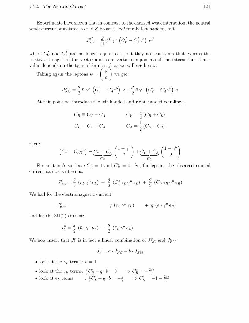
11.2. The Neutral Current 121
Experiments have shown that in contrast to the charged weak interaction, the neutralweak current associated to the Z-boson is not purely left-handed, but:
JµfNC =g
2ψf γµ
(
CfV − Cf
Aγ5)
ψf
where CfV and Cf
A are no longer equal to 1, but they are constants that express therelative strength of the vector and axial vector components of the interaction. Theirvalue depends on the type of fermion f , as we will see below.
Taking again the leptons ψ =
(
νe
)
we get:
JµNC =g
2ν γµ
(
CνV − Cν
Aγ5)
ν +g
2e γµ
(
CeV − Ce
Aγ5)
e
At this point we introduce the left-handed and right-handed couplings:
CR ≡ CV − CA CV =1
2(CR + CL)
CL ≡ CV + CA CA =1
2(CL − CR)
then:(
CV − CAγ5)
= CV − CA︸ ︷︷ ︸
CR
(
1 + γ5
2
)
+ CV + CA︸ ︷︷ ︸
CL
(
1− γ5
2
)
For neutrino’s we have CνL = 1 and Cν
R = 0. So, for leptons the observed neutralcurrent can be written as:
JµNC =g
2(νL γ
µ νL) +g
2(Ce
L eL γµ eL) +
g
2(Ce
R eR γµ eR)
We had for the electromagnetic current:
JµEM = q (eL γµ eL) + q (eR γ
µ eR)
and for the SU(2) current:
Jµ3 =g
2(νL γ
µ νL) −g
2(eL γ
µ eL)
We now insert that Jµ3 is in fact a linear combination of JµNC and JµEM :
Jµ3 = a · JµNC + b · JµEM
• look at the νL terms: a = 1
• look at the eR terms: g2CeR + q · b = 0 ⇒ Ce
R = −2qbg
• look at eL terms : g2CeL + q · b = − g
2⇒ Ce
L = −1− 2qbg
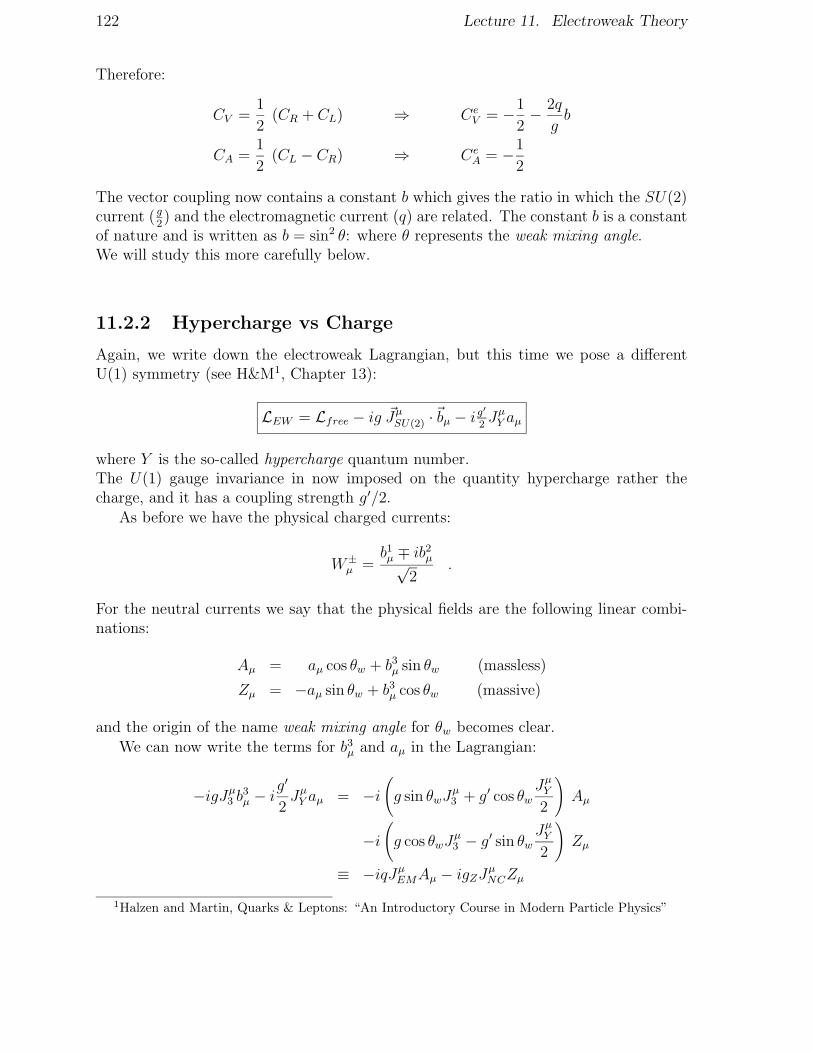
122 Lecture 11. Electroweak Theory
Therefore:
CV =1
2(CR + CL) ⇒ Ce
V = −1
2− 2q
gb
CA =1
2(CL − CR) ⇒ Ce
A = −1
2
The vector coupling now contains a constant b which gives the ratio in which the SU(2)current ( g
2) and the electromagnetic current (q) are related. The constant b is a constant
of nature and is written as b = sin2 θ: where θ represents the weak mixing angle.We will study this more carefully below.
11.2.2 Hypercharge vs Charge
Again, we write down the electroweak Lagrangian, but this time we pose a differentU(1) symmetry (see H&M1, Chapter 13):
LEW = Lfree − ig ~JµSU(2) ·~bµ − i g′
2JµY aµ
where Y is the so-called hypercharge quantum number.The U(1) gauge invariance in now imposed on the quantity hypercharge rather thecharge, and it has a coupling strength g′/2.
As before we have the physical charged currents:
W±µ =
b1µ ∓ ib2µ√2
.
For the neutral currents we say that the physical fields are the following linear combi-nations:
Aµ = aµ cos θw + b3µ sin θw (massless)
Zµ = −aµ sin θw + b3µ cos θw (massive)
and the origin of the name weak mixing angle for θw becomes clear.We can now write the terms for b3µ and aµ in the Lagrangian:
−igJµ3 b3µ − ig′
2JµY aµ = −i
(
g sin θwJµ3 + g′ cos θw
JµY2
)
Aµ
−i(
g cos θwJµ3 − g′ sin θw
JµY2
)
Zµ
≡ −iqJµEMAµ − igZJµNCZµ
1Halzen and Martin, Quarks & Leptons: “An Introductory Course in Modern Particle Physics”

11.2. The Neutral Current 123
The weak hypercharge is introuced in complete analogy with the strong hypercharge,for which we have the famous Gellmann - Nishijima relation: Q = I3 +
12YS. In the
electroweak theory we use: Q = T3 +12Y which means:
JµEM = Jµ3 + 12JµY
then, indeed, for the Aµ field we have:
−ig sin θw(
Jµ3 +g′ cos θwg sin θw
· 12JµY
)
= −ieJµEM ,
provided the following relation holds:
g sin θw = g′ cos θw = e .
The weak mixing angle is defined as the ratio of the coupling constants of the SU(2)Lgroup and the U(1)Y group:
tan θw =g′
g.
For the Z-currents we then find:
−i(
g cos θwJµ3 −
g′
2sin θw · 2 (JµEM − Jµ3 )
)
Zµ
= ...
= −i e
cos θw sin θw
(
Jµ3 − sin2 θwJµEM
)
Zµ
So we see that:JµNC = Jµ3 − sin2 θw J
µEM
which is in agreement with what we had obtained earlier:
Jµ3 = a · JµNC + b · JµEM with a = 1 and b = sin2 θw
11.2.3 Assessment
We introduce a symmetry group SU(2) ⊗ U(1)Y and describe electroweak interactionswith:
−i(
g ~JµL ·~bµ +g′
2JµY · aµ
)
The coupling constants g and g′ are free parameters (we can also take e and sin2 θw).The electromagnetic and weak currents are then given by:
JµEM = Jµ3 +1
2JµY
JµNC = Jµ3 − sin2 θwJµEM = cos2 θwJ
µ3 − sin2 θw
JµY2

124 Lecture 11. Electroweak Theory
and the interaction term in the Lagrangian becomes:
−i(
eJµEM · Aµ +e
cos θw sin θwJµNC · Zµ
)
in terms of the physical fields Aµ and Zµ.
11.3 The Mass of the W and Z bosons
In the electroweak model as introduced here, the gauge fields must be massless, since ex-plicit mass terms (∼ φµφ
µ) are not gauge invariant. In the Standard Model the mass ofall particles are generated in the mechanism of spontaneous symmetry breaking, intro-ducing the Higgs particle (see later lectures.) Here we just give an empirical argumentto predict the mass of the W and Z particles.
1. Mass terms are of the following form:
M2φ = 〈φ |H|φ〉 for any field φ
2. From the comparison with the Fermi 4-point interaction we find:
GF√2=
g2
8M2W
⇒ M2W =
√2g2
8GF
=
√2
8GF
e2
sin2 θ
Thus, we get the following predictions:
MW =
√√√√
√2
8GF
e
sin θw= 81 GeV
MZ = MW (gz/g) =MW/cos θ = 91 GeV
11.4 The Coupling Constants for Z → f f
For the neutral Z-current interaction we have in general:
−igZ JµNC Zµ = −i g
cos θw
(
Jµ3 − sin2 θwJµEM
)
Zµ
= −i g
cos θwψfγ
µ[1
2
(
1− γ5)
T3 − sin2 θwQ]
︸ ︷︷ ︸
12(C
fV−Cf
Aγ5)
ψf · Zµ
which we can represent with the following vertex:
Z0
f
f−i g
cos θwγµ
1
2
(
CfV − Cf
Aγ5)
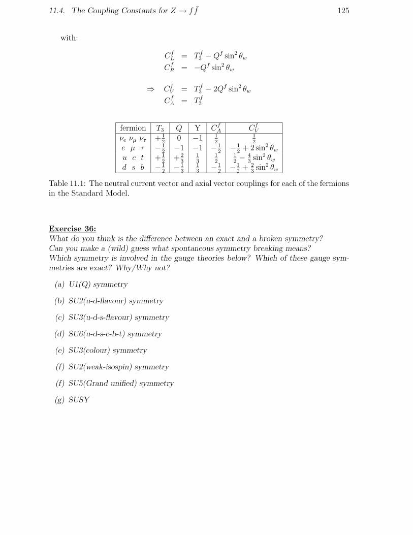
11.4. The Coupling Constants for Z → f f 125
with:
CfL = T f
3 −Qf sin2 θw
CfR = −Qf sin2 θw
⇒ CfV = T f
3 − 2Qf sin2 θw
CfA = T f
3
fermion T3 Q Y CfA Cf
V
νe νµ ντ +12
0 −1 12
12
e µ τ −12−1 −1 −1
2−12+ 2 sin2 θw
u c t +12
+23
13
12
12− 4
3sin2 θw
d s b −12−13
13
−12−12+ 2
3sin2 θw
Table 11.1: The neutral current vector and axial vector couplings for each of the fermionsin the Standard Model.
Exercise 36:What do you think is the difference between an exact and a broken symmetry?Can you make a (wild) guess what spontaneous symmetry breaking means?Which symmetry is involved in the gauge theories below? Which of these gauge sym-metries are exact? Why/Why not?
(a) U1(Q) symmetry
(b) SU2(u-d-flavour) symmetry
(c) SU3(u-d-s-flavour) symmetry
(d) SU6(u-d-s-c-b-t) symmetry
(e) SU3(colour) symmetry
(f) SU2(weak-isospin) symmetry
(f) SU5(Grand unified) symmetry
(g) SUSY
126 Lecture 11. Electroweak Theory

Lecture 12
The Process e−e+ → µ−µ+
12.1 The Cross Section of e−e+ → µ−µ+
Equipped with the Feynman rules of the electroweak theory we proceed to calculatethe cross section of the electroweak process: e−e+ → γ, Z → µ−µ+ . We assume thefollowing kinematics:
−θ
µ
µ
ee
+
−
+
Figure 12.1: Kinematics of the process e−e+ → µ−µ+.
There are two Feynman diagrams that contribute to the process:
Mγ : γ
e+
e−
µ+
µ−
MZ :Z
e+
e−
µ+
µ−
Figure 12.2: Feynman diagrams contributing to e−e+ → µ−µ+
In complete analogy with the calculation of the QED process e+e− → e+e− we obtainthe cross section using Fermi’s Golden rule:
dσ =|M|2
FdQ
With the phase factor dQ flux factor F :
dQ =1
4π2pf4√sdΩ
127

128 Lecture 12. The Process e−e+ → µ−µ+
F = 4pi√s
σ(
e−e+ → µ−µ+)
=1
64π2· 1s· |M|2
The Matrix element now includes:
Mγ = −e2 (mγµm) · gµνq2· (eγνe)
MZ = − g2
4 cos2 θw
[
mγµ(
CmV − Cm
A γ5)
m]
· gµν − qµqν/M2Z
q2 −M2Z
·[
eγν(
CeV − Ce
Aγ5)
e]
The propagator for massive vector bosons (Z-boson) is discussed in Halzen & Martin§6.11 and §6.12. The wave equation of a massless spin-1 particle is:
22Aµ = 0 ⇒ i
−gµνq2
(
22 +M2
)
Zµ = 0 ⇒ i−gµν + qµqν/M
2
q2 −M2
We can simplify the propagator of the Z if we ignore the lepton masses. In practicethis means that we work in the limit of high-energy scattering. In that case the Diracequation becomes:
(i∂µγµ −m)ψe = 0 ⇒ (γµPµ,e)ψe = 0
Since Pe =12q we also have:
1
2(γµqµ)ψe = 0 ⇒ qµ · qν/M2
z = 0
Thus the propagator simplifies:
gµν − qµqν/M2Z
q2 −M2Z
→ gµνq2 −M2
Z
Thus we have for the Z-exchange matrix element the expression:
MZ =−g2
4 cos2 θw
1
q2 −M2Z
·[
m γµ(
CmV − Cm
A γ5)
m] [
e γµ(
CeV − Ce
Aγ5)
e]
.
To calculate the cross section by summing overMγ andMZ is now straightforward buta rather lengthy procedure: applying Casimir’s trick, trace theorems, etc. Let us heretry to follow a different approach.
We rewrite the MZ matrix element in terms of right-handed and left-handed cou-plings, using the definitions: CR = CV − CA ; CL = CV + CA. As before we have:
(
CV − CAγ5)
= (CV − CA) ·1
2
(
1 + γ5)
+ (CV + CA) ·1
2
(
1− γ5)
.

12.1. The Cross Section of e−e+ → µ−µ+ 129
Thus:(
CV − CAγ5)
ψ = CRψR + CLψL .
Let us now look back at the QED process:
Mγ =−e2s
(mγµm) (eγµe)
with (see previous lecture):
(mγµm) = (mLγµmL) + (mRγ
µmR)
(eγµe) = (eLγµeL) + (eRγµeR)
The fact that there are no terms connecting L-handed to R-handed (mRγµmL) actually
implies that we have helicity conservation for high energies (i.e. neglecting ∼ m/Eterms) at the vertices:
R R L L
or:L
R
R
L
Figure 12.3: Helicity conservation. left: A right-handed incoming electron scatters intoa right-handed outgoing electron and vice versa in a vector or axial vector interaction .right: In the crossed reaction the energy and momentum of one electron is reversed: i.e.in the e+e− pair production a right-handed electron and a left-handed positron (or viceversa) are produced. This is the consequence of a spin=1 force carrier. (In all diagramstime increases from left to right.)
As a consequence we can decompose the unpolarized QED scattering process as asum of 4 cross section contributions:
dσ
dΩ
unpolarized
=1
2 dσ
dΩ
(
e−Le+R → µ−Lµ
+R
)
+dσ
dΩ
(
e−Le+R → µ−Rµ
+L
)
dσ
dΩ
(
e−Re+L → µ−Lµ
+R
)
+dσ
dΩ
(
e−Re+L → µ−Rµ
+L
)
where we average over the incoming spins and sum over the final state spins.
Let us look in more detail at the helicity dependence (H&M §6.6):

130 Lecture 12. The Process e−e+ → µ−µ+
Final state:
z−axis
z’−axis
θ
µ
µ
+
−
e+ e −
Initial state:
In the initial state the e− ande+ have opposite helicity (as theyproduce a spin 1 γ).
The same is true for the final stateµ− and µ+.
So, in the center of mass frame, scattering proceeds from an initial state with JZ =+1 or −1 along axis z into a final state with J ′Z = +1 or −1 along axis z′. Since theinteraction proceeds via a photon with spin J = 1 the amplitude for scattering over anangle θ is then given by the rotation matrices1.
djm′m(θ) ≡⟨
jm′|e−iθJy |jm⟩
where the y-axis is perpendicular to the interaction plane.
In the example we have j = 1 and m,m′ = ±1
d11 1(θ) = d1−1−1(θ) =1
2(1 + cos θ)
d11−1(θ) = d1−1 1(θ) =1
2(1− cos θ)
From this we can see that:
dσ
dΩ
(
e−Le+R → µ−Lµ
+R
)
=α2
4s(1 + cos θ)2 =
dσ
dΩ
(
e−Re+L → µ−Rµ
+L
)
dσ
dΩ
(
e−Le+R → µ−Rµ
+L
)
=α2
4s(1− cos θ)2 =
dσ
dΩ
(
e−Re+L → µ−Lµ
+R
)
Indeed the unpolarised cross section is obtained as the spin-averaged sum over theallowed helicity combinations: 1
4· [(1) + (2) + (3) + (4)] =
dσ
dΩ
unpol
=α2
8s
[
(1 + cos θ)2 + (1− cos θ)2]
=α2
4s
(
1 + cos2 θ)
.
1See H&M§2.2:e−iθJ2 |j m〉 =
∑
m′
djmm′(θ) |j m′〉
and also appendix H in Burcham & Jobes

12.1. The Cross Section of e−e+ → µ−µ+ 131
Now we go back to the γ, Z scattering. We have the individual contributions of thehelicity states, so let us compare the expressions for the matrix-elementsMγ andMZ :
Mγ = −e2
s[ (mLγ
µmL) + (mRγµmR) ] · [ (eLγµeL) + (eRγµeR) ]
MZ = − g2
4 cos2 θw
1
s−M2Z
[ CmL (mLγ
µmL) + CmR (mRγ
µmR) ] · [ CeL (eLγµeL) + Ce
R (eRγµeR) ]
Since the helicity processes do not interfere, we can see (Exercise 37 (a)) that:
dσ
dΩ γ,Z
(
e−Le+R → µ−Lµ
+R
)
=α2
4s(1 + cos θ)2 · |1 + r Cm
L CeL|2
dσ
dΩ γ,Z
(
e−Le+R → µ−Rµ
+L
)
=α2
4s(1− cos θ)2 · |1 + r Cm
RCeL|2
with:
r =g2
e21
4 cos2 θw
s
s−M2z
=
√2GFM
2Z
e2s
s−M2Z
.
where we used that:
GF√2=
g2
8M2W
=g2
8M2Z cos2 θw
.
Similar expressions hold for the other two helicity configurations.
We note that there is a strange behaviour in the expression of the cross section ofthe Z-propagator. When
√s → MZ the cross section becomes ∞. In reality this does
not happen (that would be unitarity violation) due to the fact that the Z-particle itselfdecays and has an intrinsic decay width ΓZ . This means that the cross section has aBreit Wigner resonance shape. We are not going to derive it, but refer to the literature:Perkins2.
The argument followed by H&M §2.10 goes as follows: The wave function for anon-stable massive particle state is:
|ψ (t)|2 = |ψ (0)|2 e−Γt with Γ the lifetime.
ψ (t) ∼ e−iMt e−Γ2t withM the mass.
2Perkins: Introduction to high energy Physics 3rd ed. §4.8.

132 Lecture 12. The Process e−e+ → µ−µ+
As function of the energy the state isdescribed by the Fourier transform:
χ(E) =∫
ψ(t)eiEtdt ∼ 1
E −M + (iΓ/2).
Such that experimentally we would observe:
|χ (E)|2 = A
(E −M)2 + (Γ/2)2,
the so-called Breit-Wigner resonance shape.
Breit Wigner
A=10M=20Γ=2.5
E
0
1
2
3
4
5
6
0 5 10 15 20 25 30 35 40
In the propagator for the z-boson we replace:
1
s−M2Z
→ 1
s−(
MZ − iΓZ2
)2 =1
s−(
M2Z − Γ2z
4
)
+ iMZΓZ
We observe two changes:
1. The maximum of the distribution shifts from M 2Z →M2
Z −Γ2Z
4.
2. The expression will be finite because of the term ∝MZΓZ
For our expressions in the process e−e+ → γ, Z → µ−µ+ it means that we only replace:
r =
√2GFM
2Z
e2· s
s−M2Z
by r =
√2GFM
2Z
e2· s
s−(
MZ − iΓZ2
)2
The total unpolarized cross section finally becomes the average over the four L, Rhelicity combinations. Inserting “lepton universality” Ce
L = CµL ; Ce
R = CµR and therefore
also: CeV = Cµ
V ; CeA = Cµ
A , the expression becomes (by writing it out):
dσ
dΩ=
α2
4s
[
A0
(
1 + cos2 θ)
+ A1 (cos θ)]
with A0 = 1 + 2Re(r) C2V + |r|2
(
C2V + C2
A
)2
A1 = 4Re(r) C2A + 8|r|2C2
VC2A
In the Standard Model we have: CA = −12and CV = −1
2+ 2 sin2 θ .
The general expression for e−e+ → γ, Z → µ−µ+ is (assuming seperate couplings forinitial and final state):
A0 = 1 + 2Re(r) CeVC
fV + |r|2
(
CeV2 + Ce
A2) (
CfV
2+ Cf
A
2)
A1 = 4Re(r) CeAC
fA + 8|r|2 Ce
VCeVC
fAC
fA
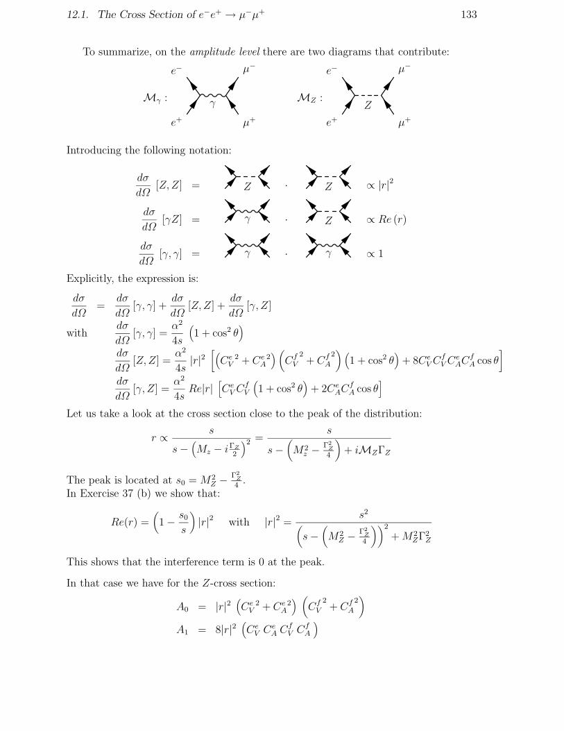
12.1. The Cross Section of e−e+ → µ−µ+ 133
To summarize, on the amplitude level there are two diagrams that contribute:
Mγ : γ
e+
e−
µ+
µ−
MZ :Z
e+
e−
µ+
µ−
Introducing the following notation:
dσ
dΩ[Z,Z] = Z · Z ∝ |r|2
dσ
dΩ[γZ] = γ · Z ∝ Re (r)
dσ
dΩ[γ, γ] = γ · γ ∝ 1
Explicitly, the expression is:
dσ
dΩ=
dσ
dΩ[γ, γ] +
dσ
dΩ[Z,Z] +
dσ
dΩ[γ, Z]
withdσ
dΩ[γ, γ] =
α2
4s
(
1 + cos2 θ)
dσ
dΩ[Z,Z] =
α2
4s|r|2
[(
CeV2 + Ce
A2)(
CfV
2+ Cf
A
2)(
1 + cos2 θ)
+ 8CeVC
fVC
eAC
fA cos θ
]
dσ
dΩ[γ, Z] =
α2
4sRe|r|
[
CeVC
fV
(
1 + cos2 θ)
+ 2CeAC
fA cos θ
]
Let us take a look at the cross section close to the peak of the distribution:
r ∝ s
s−(
Mz − iΓZ2
)2 =s
s−(
M2z −
Γ2Z
4
)
+ iMZΓZ
The peak is located at s0 =M2Z −
Γ2Z
4.
In Exercise 37 (b) we show that:
Re(r) =(
1− s0s
)
|r|2 with |r|2 = s2(
s−(
M2Z −
Γ2Z
4
))2
+M2ZΓ
2Z
This shows that the interference term is 0 at the peak.
In that case we have for the Z-cross section:
A0 = |r|2(
CeV2 + Ce
A2) (
CfV
2+ Cf
A
2)
A1 = 8|r|2(
CeV C
eA C
fV C
fA
)

134 Lecture 12. The Process e−e+ → µ−µ+
The total cross section (integrated over dΩ) is then:
σ(s) =G2FM
4Z
(
s−(
M2Z −
Γ2Z
4
))2
+M2ZΓ
2Z
· s6π
(
CeV2 + Ce
A2) (
CfV
2+ Cf
A
2)
.
Ecm [GeV]σ ha
d [n
b]
σ from fitQED unfolded
measurements, error barsincreased by factor 10
ALEPHDELPHIL3OPAL
σ0
ΓZ
MZ
10
20
30
40
86 88 90 92 94
Figure 12.4: left: The Z-lineshape as a function of√s. right: The Lineshape parameters
for the lowest order calculations and including higher order corrections.
12.2 Decay Widths
We can also calculate the decay width:
Γ(
Z → ff)
f
f
which is according Fermi’s golden rule:
Γ(
Z → ff)
=1
16π
1
MZ
∣∣∣M
∣∣∣
2
=g2
48π
Mz
cos2 θw
(
CfV
2+ Cf
A
2)
=GF
6√2
M3Z
π
(
CfV
2+ Cf
A
2)
Using this expression for Γe ≡ Γ(Z → e+e−) and Γf ≡ Γ(Z → ff) we can re-write:
σ(s) =12π
M2Z
· s(
s−(
M2Z −
Γ2Z
4
))2
+M2ZΓ
2Z
· ΓeΓf .

12.3. Forward Backward Asymmetry 135
Close to the peak we then find:
σpeak ≈12π
M2Z
ΓeΓfΓ2Z
=12π
M2Z
BR(Z → ee) ·BR(Z → ff)
Let us now finally consider the case when f = q (a quark). Due to the fact thatquarks can be produced in 3 color-states the decay width is:
Γ(Z → qq) =GF
6√2
M3Z
π
(
CfV
2+ Cf
A
2)
·NC
with the colorfactor NC = 3. The ratio between the hadronic and leptonic width:Rl = Γhad/Γlep can be defined. This ratio can be used to test the consistency of thestandard model by comparing the calculated value with the observed one.
12.3 Forward Backward Asymmetry
The forward-backward asymmetry can be defined using the polar angle distribution:
dσ
d cos θ∝ 1 + cos2 θ +
8
3Afb cos θ
This defines the forward-backward asymmetry with:
A0,fFB =
3
4AeAf where Af =
2CfVC
fA
C2V + C2
A
The precise measurements of the forward-backward asymmetry can be used to de-termine the couplings CV and CA.
0.01
0.014
0.018
0.022
20.6 20.7 20.8 20.9
Rl
A0,
l
fb
68% CL
l+l−
e+e−
µ+µ−
τ+τ−
αs
mt
mH
combined in plots with SLD resultsFigure 12.5: left: Test of lepton-universality. The leptonic Afb vs. Rl. The contoursshow the measurements while the arrows show the dependency on Standard Modelparameters. right: Determination of the vector and axial vector couplings.

136 Lecture 12. The Process e−e+ → µ−µ+
12.4 The Number of Light Neutrino Generations
Since the total decay width of the Z must be equal to the sum of all partial widths thefollowing relation holds:
ΓZ = Γee + Γµµ + Γττ + 3Γuu + 3Γdd + 3Γss + 3Γcc + 3Γbb +Nν · Γνν
From a scan of the Z-cross section as function of the center of mass energy we find:
ΓZ ≈ 2490 MeV
Γee ≈ Γµµ ≈ Γττ = 84 MeV CV ≈ 0 CA = −1
2
Γνν = 167 MeV CV =1
2CA =
1
2
Γuu ≈ Γcc = 276 MeV CV ≈ 0.19 CA =1
2
Γdd ≈ Γss ≈ Γbb = 360 MeV CV ≈ −0.35 CA = −1
2
(Of course Γtt = 0 since the top quark is heavier than the Z.)
Nν =ΓZ − 3Γl − Γhad
Γνν= 2.984± 0.008 .
Figure 12.6: The Z-lineshape for resp. Nν = 2, 3, 4.

12.4. The Number of Light Neutrino Generations 137
Figure 12.7: Standard Model fit of the predicted value of the Higgs boson.

138 Lecture 12. The Process e−e+ → µ−µ+
Exercise 37:
(a) Show how the unpolarised cross section formula for the process e+e− → Z, γ → µ+µ−
can be obtained from the expression of the helicity cross sections in the lecture:
dσ
dΩ
(
e−L/Re+R/L → µ−L/Rµ
+R/L
)
=α2
4s(1± cos θ)2
∣∣∣1 + r Ce
L/RCµL/R
∣∣∣
2
(b) Show, using the expression of r from the lecture, that close to the peak of theZ-lineshape the expression
Re(r) =(
1− s0s
)
|r|2
with s0 =M2z − Γ2z/4 holds.
(c) Show also that at the peak:
σpeak ≈12π
M2z
ΓeΓµΓZ
(d) Calculate the relative contribution of the Z-exchange and the γ exchange to thecross section at the Z peak.Use sin2 θW = 0.23, Mz = 91GeV and ΓZ = 2.5GeV .
(e) The actual line shape of the Z-boson is not a pure Breit Wigner, but it is asym-metrical: at the high
√s side of the peak the cross section is higher then expected
from the formula derived in the lectures.Can you think of a reason why this would be the case?
(f) The number of light neutrino generations is determined from the “invisible width”of the Z-boson as follows:
Nν =ΓZ − 3Γl − Γhad
Γν
Can you think of another way to determine the decay rate of Z → νν directly?Do you think this method is more precise or less precise?