r -

NASA Technical Memorandum 103288

Particle Displacement Trackingfor PIV

Mark P. Wernet

Lewis Research Center

Cleveland, Ohio

September 1990

(NAS A-TM-].032_8)

" TRACKING FOR PlY

PARTICLE _ISPLACEMENT

(NASA) 25 p CSCL 14B

G3/35

NqI-IOZTI

https://ntrs.nasa.gov/search.jsp?R=19910000958 2020-06-06T23:39:07+00:00Z

_._, "--" _-_--- _T=:= _¸ _='=_-'_ _=_ _=i

_= 9

f

PARTICLE DISPLACEMENT TRACKING FOR PIV

Mark P. Wernet

National Aeronautics and Space AdministrationLewis Research Center

Cleveland, OH 44135

Abstract

A new PIV data acquisition and analysis system, which is an order of magnitude

faster than any previously proposed system has been constructed and tested. The new

Particle Displacement Tracking (PDT) system is an all electronic technique employing a

video camera and a large memory buffer frame-grabber board. Using a simple encoding

scheme, a time sequence of single exposure images are time coded into a single image and

then processed to track particle displacements and determine velocity vectors. Application

of the PDT technique to a counter-rotating vortex flow produced over 1100 velocity

vectors in 110 seconds when processed on an 80386 PC.

Particle Imaging Velocimetry (PIV) is a very useful tool in the study of transient

fluid flow phenomena. Many classes of engineering problems satisfy the in-plane velocity

requirements of the technique. The processing techniques for reducing PIV data have

traditionally been tedious and time consuming. Hence, much effort continues to be

devoted to developing more refined and expedient data reduction techniques. In this work

a new approach to PIV data reduction is presented which uses a simple space domain

particle tracking algorithm.

J

In PIV, pulsed light sheets are used to record the in-plane positions of particles

entrained in the flow at two instances in time. i Low particle concentrations are used to

ensure that individual particle images are clearly resolved. 2 Subsequent processing of the

photographically recorded particle images yields a 2-D velocity vector map across an

extended planar cross section of the flow. A common data reduction technique is the beam

readout technique. 3-4 Other techniques involve digitizing small sections of the photograph

and performing numerically intensive computations or employ image processors to detect

velocity vectors. 5-8 All of the photographic recording PIV techniques offer high precision

estimates of the velocity, but require extremely long processing times even on specialized

array processors. Chemical processing of the exposed plates is a cumbersome and tedious

process. The photographic plates must also be stored and catalogued.

%

Other PIV work has focused on developing all electronic acquisition and processing

systems. Electronic recording and processing offers the advantages of no chemical

processing steps, and no large volumes of photographic plates to catalog, store, or break.

The most attractive features are system integration and simplicity. In a electronic PIV

system, all of the data acquisition and processing can be performed on a single computer.

No media conversion is required. The comparatively low resolution of video cameras to

that of photographic film limits the spatial resolution of electronic PIV recording

techniques. However, if small (50,,50 mm) cross sections of the flow are imaged, the spatial

resolution of video cameras is acceptable.

All of the electronic PIV work has been concerned with resolving individual particle

images and/or particle streaks. In some of the previous electronic PIV work, particle

streaks were digitally recorded and later image processed to estimate the streak lengths. 7

Combinations of streaks and dots have also been employed to determine the velocity vector

direction. 8 Other electronic PIV systems use multiple exposures (> 2) on a single image,

2

and then rely on the operator to visually recognize particle displacement records. 9 The

recognized particle image sets are marked using an image processor cursor and stored in the

computer.

The Particle Displacement Tracking (PDT) technique uses a time sequence of single

exposure images to determine direction information and to track particles. Time sequences

of particle images to estimate velocity have been previously proposed and analyzed in

computer simulations. 10-11 However, cross---correlation and FFT techniques were used to

obtain velocity magnitude, which are both computationally intensive operations. The

cross-correlation technique yields the velocity vector direction information in conjunction

with the vector magnitude. In the FFT approach, the sequence of single exposure particle

image frames are linearly superimposed to generate a single multiple exposure record,

which is then Fast Fourier Transformed to estimate the velocity vector magnitude. The

sequence of single exposure images is used as a phase reference, so that the direction

information can be inferred.

The PDT technique has evolved from a previous work on a 'Vector Scanning' space

domain processing technique. 1_ In this previous work, a sequence of single exposure images

were used to estimate velocity vectors. A particle displacement pattern was selected, and

then scanned through the entire image. The only difference between the PDT technique

and the previous work is the algorithm used to detect the occurrence of velocity vectors.

The PDT system is an order of magnitude faster than the previous vector scanning

technique.

The Vector Scanning and PDT techniques are the only fully automatic electronic

PIV systems yet devised. In all other PIV systems, some operator intervention or

supervision is required either at data recording or during data reduction. In the Particle

3

DisplacementTracking (PDT) system, no operator intervention is required in the data

reduction process as long as good quality, high contrast PIV images are recorded. If the

contrast is not optimal, then the appropriate threshold level to eliminate the background

level is the only operator intervention required.

The PDT technique uses a simple algorithm which utilizes the time sequence of

particle image fields to determine both the velocity vector magnitude and direction,

without numerically intensive operations. All computations can be performed on a PC.

The PDT technique is demonstrated on a counter-rotating convection vortex flow. Over

1100 velocity vectors were detected in a 50,, 100 mm field of view and completely processed

on an 80386 PC in 110 seconds.

Particle Displacement Tracking

The Particle Displacement Tracking (PDT) technique is applicable only to low

velocity PIV fluid flow systems. In the PDT system, a cw laser source is used to generate

a light sheet, and a video array camera/frame---grabber board records the particle image

data. The frame-grabber board is used to acquire five video fields equally spaced in time

from the RS-170 video source. The choice of five fidds minimizes the error rate in

subsequent processing.l_ The time interval, AT, between recorded fields is 1/60 second at

the minimum, and essentially unlimited at the maximum time interval, which corresponds

to the minimum velocities. The actual value of AT is selected according to the fluid

velocities of interest. The particle seeding number density is selected so that the individual

particle images are clearly imaged. The recorded particle images do not overlap.

The five video fields are then individually processed to determine the centroid

location of each particle image on each video field in the sequence. The particle image

4

,J

centroids are estimated to within • ½ pixel.12 Although the particle positions are actually

estimated to sub-pixel accuracy, at this point in the PDT development the need for high

precision particle position estimates is not required. A simple boundary following

algorithm with centroid estimation is used to estimate the particle locations. The details

of the centroid processing are discussed in reference 12. The single pixel particle centroid

estimates from all of the particle images recorded in the five field sequence are combined

into a single 640x480x8 bit square pixel image. The time history of each particle image is

encoded in the amplitude of the pixei marking the position of the particle centroid. The

pixel amplitudes are coded according to the time order in the five field sequence. All of the

particle centroids from video field #1 are encoded into the composite image as pixels with

amplitudes 2 I. Similarly, particle centroids from video field #2 are encoded with

amplitude 2 _. By amplitude coding the pixel locations of the particle centroids, a single

image is generated which contains the time history displacements of all the particles

recorded in the five field sequence over a total time interval of 4AT. Figure 1 shows two

particle image displacement records encoded into a 100xl00 pixel image. The amplitudes

of the pixels marking the centroid positions increase from 21 at T--0, and 2 5 at T=4AT.

Amplitude coding unambiguously defines the particle's direction of travel. The amplitude

coding also decreases the probability of mistakenly identifying a particle image from a

different particle as being part of another particle displacement record. Another advantage

of using single exposure particle images fields is the elimination of particle image overlap,

which typically restricts the lower limit of velocities which can be measured. By

individually processing the particle image fields, particle images with large diameters

relative to their displacement between exposures are easily tolerated. The only constraint

on the minimum velocity is that the particle must travel at least one pixel between

exposures.

The time history image serves as the input to the PDT algorithm. The PDT

algorithm begins by scanning the time history image and storing the locations of all pixels

with amplitude 2 l, which corresponds to all particle positions at the initial field in the

sequence. The particle positions at T=0 serve as the starting point for the displacement

tracking. By determining the displacement of the particle from its initial position, the

velocity information of the flow is inferred.

For each initial particle position, a circular search region is defined around the 2 l

amplitude pixel. Inside the search region, the coordinates of all pixels with amplitudes

equal to 2 2 are scanned and stored. The 2 _ amplitude coded pixels correspond to the

particle positions at T=IAT, or exposure #2. The detected 2 2 amplitude pixels within the

search region are now each successively analyzed. The distance and angle between each 2 _

amplitude pixel and the search region center 21 amplitude pixel is computed and used to

project where the 2 s, 2 4, and 2 s amplitude pixels are located which correspond to the 21 and

2 _ amplitude pixel particles; see figure 2. If the projected pixel locations for the 3 rd, 4 th,

and 5th particle images contain the corresponding amplitudes (2 3, 2 4, 2 5) then a complete

particle displacement record has been detected. The velocity vector associated with this

particle is computed from the distance between the initial and final particle locations (21

and 2 5 amplitude pixels), and the sum of the four inter--exposure intervals (4AT). The

detected particle pixel amplitudes are then set to zero. If the projected particle locations

detect the incorrect pixel amplitude or zero amplitude, then the 2 2 amplitude pixel within

the search region is not the actual second image of the 21 amplitude pixel at the center of

the search region. Each 2 2 amplitude pixel within the search region is examined until a

complete particle displacement pattern is detected or all of the 2 2 amplitude pixels are

exhausted. If no match is found, the algorithm continues on to the next initial particle

position 21 amplitude pixel. In summary, for each 21 amplitude pixel, a circular search

region is defined about that particle. All 2 2 amplitude pixels within the search region are

assumed to be the position of the initial particle at the second exposure, and thus used to

predict the successive locations of the particle at time sequence exposures 3, 4, and 5. No

preknowledge about the flow system is required. The PDT system assumes that 22

amplitude pixels in the neighborhood of the initial 21 amplitude pixel are the most probable

particle displacements between video fields #1 and #2 in the five field sequence. The

maximum allowable particle displacement between exposures has previously been

determined to be 10 pixels for sharply turning flows. 12 Ten pixel displacements between

exposures minimizes the deviation of the particle path from a linear trajectory. Therefore,

the search region size is defined to be a circle of radius 10 pixels; see figure 2.

The positioning error on the discrete grid must be accommodated in the PDT

processing. As previously mentioned, the boundary processing technique provides particle

centroid estimates to within • ½ pixel on the 640,`480 pixel time history image. For each

projected particle position (for exposures 3, 4, 5) a 3,,3 pixel search region is defined. The

3,,3 search regions are centered on the projected positions; see figure 2. The expanded

regions allow for the positioning error of * ½ pixel. However, when a complete particle

displacement pattern is detected, the exact location of the amplitude coded pixel within the

3x3 region is determined and used to determine the velocity vector magnitude. The

velocity vector angle is computed from the position of the 21 and 25 amplitude pixels.

There are two sources of error in the PDT estimated velocities: 1) the particle

positioning error; and 2) the time interval error. The time interval error is minimal, since

the frame---grabber board is genlocked to the RS-170 video signal from the video camera.

The major source of error is from the particle centroid estimates. The total relative error

in the measured velocity is given by: 12

(i)

where U is the estimated mean velocity magnitude, X is the total particle displacement

from the first to last exposures, T is the sum of the four time intervals 4AT, a× is the rms

error in the total particle displacement, and aT is the timing error. For the • ½ pixel

positioning error, the rms error in the total displacement is simply 1/¢2 pixels. A nominal

estimate for the time interval error is one video scan line per acquired field, or roughly

5x65psec. Hence, for a 40 pixel total displacement and a total time interval of 2 seconds,

the relative error in the estimated velocity is:

(2)

or

= 0.018

which is dominated by the positioning error. For the worst case corresponding to only a 4

pixel total displacement, the relative error in the estimated velocity magnitude is a factor

of 10 larger, or adU = 0.18.

The error in the estimated velocity vector angle is similar to the magnitude error.

The angular error is given by: Is

if0= ARCTAN[_r _](3)

where X and a× are the particle displacement and rms error in the particle displacement,

respectively. Using the same displacement of 40 pixels, the angular error is:

o'o= ARCTAN [_--]

0"0= 1.0 °

(4)

The worst case for the angle estimates is for the smallest displacements. The minimum

displacement of 4 pixels yields an error of o'0 "- 10.0 °.

A unique feature of the PDT technique is afforded by the use of a large memory

buffer frame-grabber board which can digitize individual fields at 1/60 second intervals

and store 25 sequentially acquired video fields. The 25 fields are grouped in successive sets

of 5 fields and processed by the PDT technique described above. The five groups of 5

successive fields produce five 2-D velocity vector maps. Particles are tracked across all

five groups, for all 25 fields. Hence, the composite 2-D velocity vector map will track

particles for all five sampling intervals. Particles tracked for all 25 fields will be

represented by a string of velocity vectors oriented head to tail, which indicates the

particle path over the total measurement time of 24AT. Alternatively, the five 2-1)

velocity vector data sets can be successively displayed quickly on a computer screen to

elucidate the flowing fluid pattern. Flowing fluid five frame movies of a time stationary

flow system have been constructed; unfortunately, they cannot be displayed in this paper.

,aaip_m_e

The flow system used in this validation of the PDT technique is a prototype

configuration of a future space shuttle mission called the Surface Tension Driven

Convection Experiment (STDCE). The purpose of the experiment is to study the behavior

of heated free surface fluid flows in the absence of gravity. In the STDCE configuration

discussed here, a lcm diameter tubular heater is inserted into a cylindrical reservoir filled

with silicone oil and seeded with 200/_n pliolite particles. The silicone oil is index matched

to the plexiglas reservoir. The reservoir width to height dimensions are 2:1, the width

being 10cm. A 5 mW HeNe laser is used to provide a lmm thick light sheet, which

illuminates a radial cross section of the reservoir from the top; see figure 3. In operation,

the tubular heater drives a toroidal convection cell flow, whose cross section appears as two

counter rotating convection vortices. A Silicon Intensified Target (SIT) camera, oriented

at 90_ to the plane of the light sheet, is used to supply RS---170 video signals of the particle

images. The exposure time of the SIT camera is 1/60 second.

An EPIX 4---MEG video frame-grabber board digitizes and stores the PIV images.

The frame-grabber board is equipped with a 12.5MHz A/D oscillator so that interlaced

640x480 square pixel frames are digitized. The frame---grabber board can be configured to

digitize individual fields or frames. In field mode the minimum sampling time is 1/60

second. When acquiring video fields, 27 fields can be acquired and stored in the 4

Megabyte on-board memory buffer. However, by using just fields, the vertical resolution

is halved, producing a 640 pixel x 240 line image. The 240 lines are the even or odd fields

from the RS-170 interlaced video signal. The reduced vertical resolution decreases the

accuracy of the particle centroid estimates in the vertical direction, compared to the

horizontal direction. The reduced vertical sampling is not a significant effect if the particle

images encompass several pixels across their diameters.

The data acquisition software allows the selection of the inter-field acquisition time

interval in multiples of 1/60 second. For low velocity flows many video fields are allowed

to elapse between successively acquired images. For faster flows, adjacent fields can be

10

acquired resulting in the minimum AT of 1/60 second. When acquiring adjacent fields, a

gated camera is required to obtain sharp particle images, otherwise particle streaks will be

recorded instead. For a 100xl00 mm field of view, the image scale is roughly 175/_rn/pixel.

At the minimum inter-exposure interval of 1/60 second, the maximum measurable velocity

is roughly 100 ram/second.

The data acquisition and PDT processing are all performed on a 25MHz 80386

computer with a Weitek 3167 coprocessor. All of the PDT processing routines are written

in Fortran 77 and compiled with a 32 bit Weitek supported compiler. Video images are

stored on the hard disk and later transferred to removable cartridge disks for archiving.

Results and Discussion

A VttS video tape was made of the counter rotating convection vortex flow. Two

25 field data sets were digitized from the video tape. Each set of 25 fields were used to

generate five sets of time evolved velocity vector maps. The first data sequence was

obtained using a AT of 60 fields or 1 second intervals between successively acquired fields.

The second data sequence was acquired with a AT of 30 fields, or 1/2 second intervals.

Using two data sequences will effectively double the dynamic range in the measured

velocity magnitudes. The PDT technique limits the maximum particle displacement

between acquired fields to 10 pixels, thus the dynamic range is 10:1 for a single sequence.

By digitizing two sequences with a AT ratio of 2:1, the dynamic range of the combined

2-D velocity vector maps will be doubled, or 20:1.

A sample image field obtained from the PDT system is shown in figure 4. Only the

region within the fluid reservoir is shown, which corresponds to a digitized image size of

580 pixels ,, 143 lines. The scale of the digitized image is 172 #m/pixel. The recorded

11

particle images were approximately <10 pixels in diameter, and their recorded intensities

spanned essentially all of the 0-255 dynamic range. The tubular heater used to drive the

flow was not placed exactly in the center. The amount of decentration is not obvious in

figure 4, but will be evident in the 2-D velocity vector maps.

The acquired data sequences were boundary processed to determine the particle

image centroids. A threshold level of 10 grey levels was used for all of the boundary

processing. 12 For data sequence #1 the total boundary processing for all 25 fields was 45

seconds and approximately 320 particle centroids were detected on each field in the

sequence. For data sequence #2, the total boundary processing time was 45 seconds with

roughly 265 particles detected per video field. Next, the PDT processing was performed on

the 10 time history encoded files generated from the boundary processing stage. The total

PDT processing time was 16 seconds for all 10 images, or roughly 1.6 seconds per time

history file. Hence, for a single five field image sequence, the total boundary

processing/PDT processing time is roughly 11 seconds per data set. In the current

discussion, each data sequence of 25 fields contained five data sets. For data sequence #1,

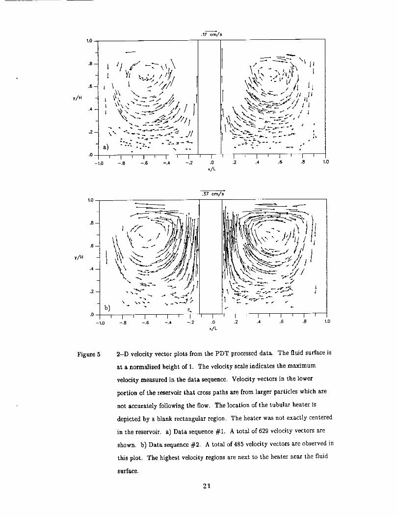
a total of 629 velocity vectors were found; see figure 5a. For data sequence #2,485

velocity vector were detected; see figure 5b. The velocity magnitude scales in both figures

5a and 5b are identical. In both 2-D velocity vector maps, sets of velocity vectors tail to

head are observed. These are the velocity vectors from particles which were tracked over

all 25 fields. The continuous tracking of particles can be used to make movies of the

evolving flow as described above.

In the counter rotating flow, the velocity is lowest in the lower outside edges of the

reservoir. The highest velocities occur next to the tubular heater near the fluid surface.

Data sequence #1, with AT=I second, shows more of the slow velocity vectors in the

outside corners of the reservoir, and few velocity vectors next to the heater near the fluid

12

v

surface. Data sequence #2, with AT=l/2 second, contains fewer slow velocity vectors in

the outside corners of the reservoir, but does show the higher velocities next to the heater

near the fluid surface. The two data sets are combined in figure 6. A good sampling of

both the high and low velocity vector magnitudes are contained in the combined data set.

Figure 6 contains a total of 1114 velocity vectors. The minimum and maximum measured

velocities were 0.17 Jr 0.03 mm/s and 3.8 • 0.06 mm/s, respectively. The error in the

measured velocity vectors is proportional to the reciprocal of the total displacement. 12 The

measured dynamic range in velocity magnitude for the combined data sequences was 22:1.

The dynamic range is higher than expected due to the use of the 3_3 pixel search regions

about the projected particle positions. The 3x3 pixel regions allow for 11 pixel

displacements. There are a few falsely identified velocity vectors in figures 5a and 5b. The

false identifications have occurred in regions of small displacement and high particle

concentration. Some of the velocity vectors in the lower portion of the cell point

downwards. These are not necessarily all false vectors, but are large particles which are

settling out of the fluid. The falsely identified velocity vectors can be eliminated using

smoothing techniques.

The randomly sampled data obtained using the PDT processing technique can be

replotted on a regular grid using a simple interpolation technique. The 11 nearest

neighbors to the grid point are used in a least squares estimate of the grid point velocity

magnitude and direction. A 2-D, 32=32 interpolated grid of velocity vectors from the

combination of data sequences #1 and #2 is shown in figure 7. The interpolated data

clearly show the features of the counter-rotating vortex flow. The flow field is very

symmetric about the tubular heater. The maximum velocities are observed along the fluid

surface adjacent to the heater. The contribution from any falsely identified velocity

vectors is diluted by the interpolation technique, yielding a good overall representation of

the fluid pattern.

13

The PDT techniquehasbeenshownto be a fully automated electronic PIV data

acquisition and analysis system. Video cameras have been shown to provide reasonably

accurate velocity vector estimates. By using a large memory buffer frame-grabber board,

25 field image sequences are acquired and five frame movies can be generated.

Alternatively, all five 2-D velocity vector maps can be combined into a single 2-D velocity

vector map. All of the data acquisition and processing were performed on an 80386 PC.

No array processors or other processing equipment was required. The total processing time

was 11 seconds per data set. Ten data sets were processed and combined to produce a 2-D

velocity vector map containing 1114 velocity vectors. Work is continuing on the PDT

technique to make high velocity (>10m/s) measurements just as fast and simple as

demonstrated herein. Also, the accuracy of the velocity estimates can be improved by

encoding the sub-pixel particle positions in the amplitude coding.

The author wishes to thank A. D. Pline for the use of the STDCE experimental

setup, and L. J. Goldman for valuable discussions.

14

1) Meynart, R.;'Instantaneous velocity field measurements in unsteady gas flow by

speckle velocimetry", AppI. Opt. 22, 535---540 (1983).

2) R. J. Adrian, C. S. Yao,"Pulsed Laser Technique Application to Liquid And Gaseous

Flows And The ScatteringPower of Seed Materials", Appl. Opt. 24, 44-52 (1985).

3) L. Lourenco, A. Krothapalli,"Particle Image Displacement Velocimetry

Measurements of a Three--Dimensional Jet", Phys. Fluids 31, 1835-1837 (1988).

4) R. J. Adrian, C. S. Yao,'Development of Pulsed Laser Velocimetry (PLV) for

Measurement of Fluid Flow", in Proceedings, Eighth Biennial Symposium on

Turbulence, X. B. Reed, Jr., J. L. Kakin, and G. K. Patterson, Eds., 170-186 (U.

Missouri Rolla 1983).

s) L. P. Goss, M. E. Post, D. D. Trump, B. Sarka, C. D. MacArthur, G. E.

Dunning, Jr.,"A Novel Technique for Blade--to-Blade Velocity Measurements in a

Turbine Cascade", 25 th Joint Propulsion Conference, AIAA---89-2691, (1989).

6) Y. C. Cho, B. G. McLachlan,"Personal Computer Based Image Processing Applied to

Fluid Mechanics Research", SPIE Applications of Digital Image Processing 829,

253--257 (1987).

7) K. A. Marko, L. Rimai,"Video Recording and Quantitative Analysis of Seed Particle

Track Images in Unsteady Flows", Appl. Opt. 24, 3666-3672 (1985).

15

s) B. Khalighi, Y. H. Lee,"Particle Tracking Velocimetry: An Automatic Image

Processing Algorithm", Appl. Opt. 28, 4328---4332 (1989).

9) C. Batur, M. J. Braun,"Measuring Flow With Machine Vision", INTECH, 34-38

(May 1989).

10) B.R. Frieden, C. K. Zoltani,"Fast Tracking Algorithm for Multiframe Particle

Image Velocimetry Data", Appl. Opt. 28, 652--655 (1989).

11) Y.C. Cho,"Digital Image Velocimetry", Appl. Opt. 28, 740-748 (1989).

12) M.P. Wernet, R. V. Edwards,"A New Space Domain Processing Technique for

Pulsed Laser Velocimetry", Appl. Opt. 29, 3399-3417 (1990).

16

Figure 1 Two amplitude coded particle displacement patterns are shown in a 100_ 100

pixel grid. Particle positions from the video fields are determined to within a

single pixel. The time order of a detected particle is coded in the pixel

amplitude. Particles from field #1 are given amplitude 2 _,particles from

field #2 are assigned amplitude 2 _, and so on for all five fields.

17

Figure 2 The PDT technique determines velocity vectors by defining a circular search

region around each 21 amplitude pixel. All 2_ amplitude pixels within the

search region are detected. The distance and angle from the 2 _amplitude

pixel and all detected 2 2 amplitude pixels is used to project where the

subsequent 3 rd, 4th, and 5th exposure particle images will occur. The

projected 3_3 pixel search regions are indicated in the figure.

18

LIGHT SHEET

CW-LASER

_--- CYLINDRICAL LENS

RESERVOIR----,_

TUBULAR HEATER

FRAME-GRABBER

5-FIELDTIME SEQUENCE

I

"",- _T ---,,-'-

Figure 3 Schematic view of the light sheet illumination, fluid flow reservoir, and data

acquisition and processing system. The tubular heater in the reservoir drives

the flow. The frame-grabber board digitizes a sequence of video fields

separated by AT, which is defined in integral multiples of 1/60 second.

19

Figure 4 A sample video field acquired from the flow system. The particle images are

10 pixels and less in diameter. The image includes only the bounding edges

of the fluid reservoir. The dark band in the center region of the reservoir

marks the location of the tubular heater.

2O

1.0

.8

.6

y/H

.4

.0

a)I

-1.0

,/ --__i? _ -. ,,_.\i Y_,...;,;zlY/

\\. _ 7 i.il/l .

.-W-'s/i l.. _J_x4/// I

I I I I I i I

-.8 -.6 -.4 -.2

.17 cm/s

I

.0

xlL

i I I 1 i 1 t I i

.2 .4 .6 .8 1.0

1.0

.6

.. ...-.---_,-I

b) " " _...0 i 1 i I i I i I

.37 cmls

Rtt,\ sI _ "_,"_ _"-_."'-- _ _... _/_i,

i I I I i 1 i I I I i

- 1.0 -.8 -.6 -.4 -.2 .0 .2 .4 .6 .8 1.0

x/L

Figure 5 2-D velocity vector plots from the PDT processed data. The fluid surface is

at a normalized height of 1. The velocity scale indicates the maximum

velocity measured in the data sequence. Velocity vectors in the lower

portion of the reservoir that cross paths are from larger particles which are

not accurately following the flow. The location of the tubular heater is

depicted by a blank rectangular region. The heater was not exactly centered

in the reservoir, a) Data sequence #1. A total of 629 velocity vectors are

shown, b) Data sequence #2. A total of 485 velocity vectors are observed in

this plot. The highest velocity regions are next to the heater near the fluid

surface.

21

-1.0 -.8 -.6 -.4 -.2 .0 .2 .4 .6 .B 1.0x/L

Figure 6 Combined data sequences #1 and #2. A large dynamic range of velocities

have been recorded. Many sets of tail to head velocity vectors are observed,

indicating particles which were tracked over the entire sampling period.

y/H

1.0

.8-

.4

.0

_ _ it. ttil,

i

7

J

.37 cm/s"

i 1 t I I 1 t 1 I I 1 i I t I i I I- 1.0 -.8 -.6 -.4 -.2 .0 .2 .4 .6 .8

×/L

1.0

Figure 7 Interpolated 2"D velocity vector plot. The combined data from sequences

#1 and #2 have been interpolated over a 32x32 grid. The interpolated data

dearly show the counter rotating flow pattern.

22

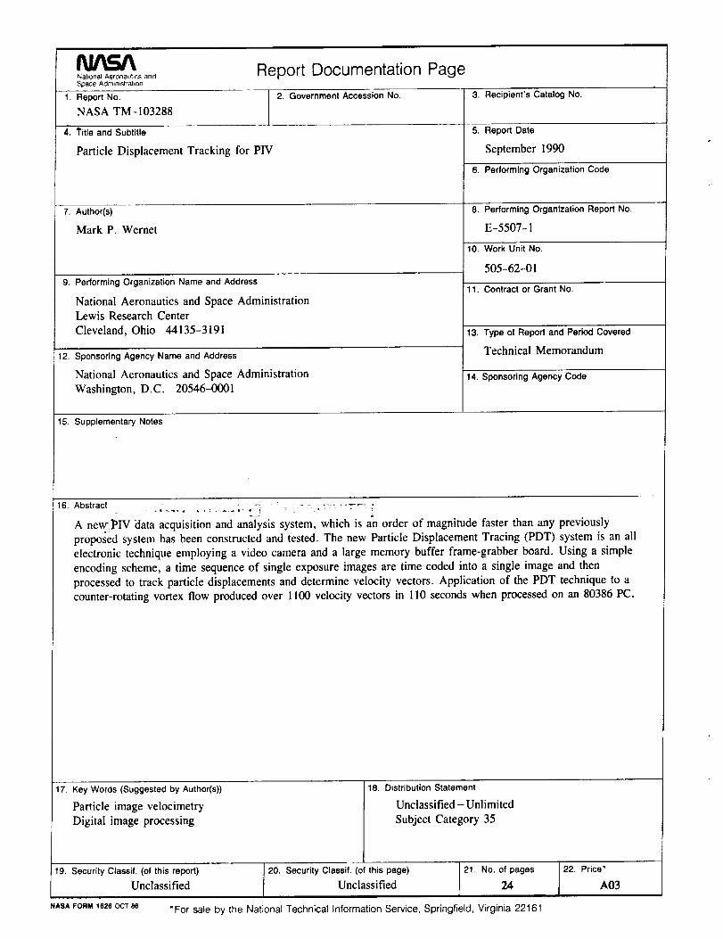
Report Documentation PageNalional Aeronautics andSpace Administralion

1. Report No.

NASA TM-103288

'41 Title and Subtitle

Particle Displacement Tracking for PIV

7. Author(s)

Mark P. Wernet

2. Government Accession No.

9. Performing Organization Name and Address

National Aeronautics and Space AdministrationLewis Research Center

Cleveland, Ohio 44135-3191

12. Sponsoring Agency Name and Address

National Aeronautics and Space Administration

Washington, D.C. 20546-0001

3. Recipient's Catalog No.

5. ReportDate

September 1990

6. Performing Organization Code

8. Performing Organization Report No.

E-5507-1

10. Work Unit No.

505-62-01

11. Contract or Grant No.

13. Type of Report and Period Covered

Technical Memorandum

14. Sponsoring Agency Code

15. Supplementary Notes

16. Abstract : ...... "....... _-_ _

A new-_PIV_data acquisition and analysis system, which is an order of magnitude faster than any previously

proposed system has been constructed and tested. The new Particle Displacement Tracing (PDT) system is an all

electronic technique employing a video camera and a large memory buffer frame-grabber board. Using a simple

encoding scheme, a time sequence of single exposure images are time coded into a single image and then

processed to track particle displacements and determine velocity vectors. Application of the PDT technique to a

counter-rotating vortex flow produced over 1100 velocity vectors in 110 seconds when processed on an 80386 PC.

17. Key Words (Suggested by Author(s))

Particle image velocimetry

Digital image processing

t9. Security Classif. (of this report)

Unclassified

18. Distribution Statement

Unclassified - Unlimited

Subject Category 35

20. Security Classif. (oi this page)

Unclassified

21. No, of pages 22. Price*

24 A03

NASAFORM1626OCT86 *For sale by the National Technical Information Service, Springfield, Virginia 22161