participation in imf programs and income...
TRANSCRIPT
Draft; not for quotation
Participation in IMF Programs and Income Inequality
Patrick Conway Department of Economics University of North Carolina Chapel Hill, NC 27517 15 January 2007
Abstract In this paper, I present an empirical analysis of the determinants of income distribution in 108 developing countries over the period 1988 to 1998. The data are the developing-country subset of those used by Milanovic (2005), augmented by information on the cumulative prior participation of the country in IMF programs over the preceding 10 years. Just as in Li et al. (1998), I conclude that the majority of variation in income inequality is cross-cross country in nature: this component of income inequality will depend primarily upon the development characteristics of the countries, and not on participation in IMF programs. I also find, however, that cumulative past participation in IMF programs has a positive effect on the share of income held by the lowest quintile of the population in those countries for which observations are available at different times. This effect is robust to the inclusion of other developmental indicators. Key words: IMF programs, income inequality, Kuznets U hypothesis JEL classifications: F33, O15
Thanks to Jim Boughton for encouraging this line of research, and to Branko Milanovic for making the data used in this paper available.
The IMF and Income Inequality - 2
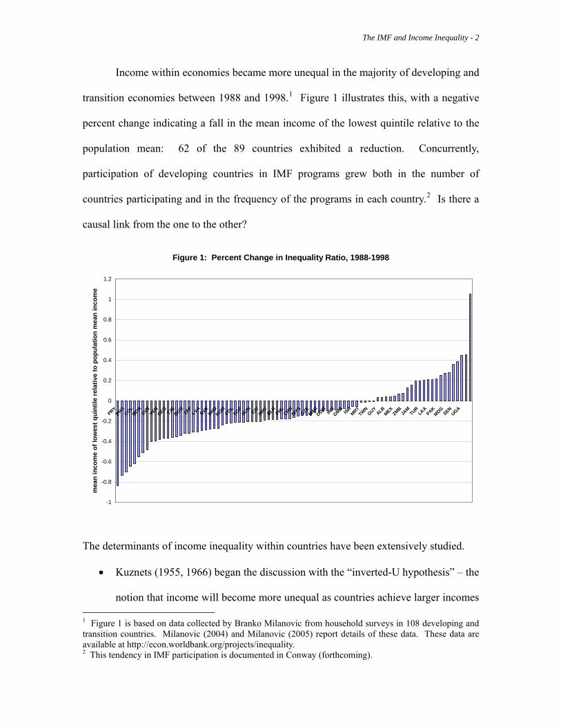
Income within economies became more unequal in the majority of developing and
transition economies between 1988 and 1998.1 Figure 1 illustrates this, with a negative
percent change indicating a fall in the mean income of the lowest quintile relative to the
population mean: 62 of the 89 countries exhibited a reduction. Concurrently,
participation of developing countries in IMF programs grew both in the number of
countries participating and in the frequency of the programs in each country.2 Is there a
causal link from the one to the other?
Figure 1: Percent Change in Inequality Ratio, 1988-1998
-1
-0.8
-0.6
-0.4
-0.2
0
0.2
0.4
0.6
0.8
1
1.2
PRYPNG
COLMDA
SVNVEN
GEOTJK BGR
ZAFLVA
SVKHND
ROMPOL
SGPHUN CIV
HRVBLR
PHLCHN
MYSCZE
MARDOM IN
DGMB ISR
MRTTWN
GUYALB
MEXZMB
JAM
TURLKA
PAKMDG
SENUGA
mea
n in
com
e of
low
est q
uint
ile re
lativ
e to
pop
ulat
ion
mea
n in
com
e
The determinants of income inequality within countries have been extensively studied.
• Kuznets (1955, 1966) began the discussion with the “inverted-U hypothesis” – the
notion that income will become more unequal as countries achieve larger incomes 1 Figure 1 is based on data collected by Branko Milanovic from household surveys in 108 developing and transition countries. Milanovic (2004) and Milanovic (2005) report details of these data. These data are available at http://econ.worldbank.org/projects/inequality. 2 This tendency in IMF participation is documented in Conway (forthcoming).

The IMF and Income Inequality - 3
per capita up to a watershed level of income per capita, and then will become
more equal with further development. The evidence for this hypothesis has
typically been cross-country in nature: ranking the countries j in ascending order
by income per capita, the inequality measure for small income per capita will
worsen as income per capita increases until a turning point, and then will grow
larger on average for countries with still higher per capita income.
• Li et al. (1998) finds in an unbalanced panel of Gini coefficients of middle- and
low-income countries that the cross-country differences in income inequality
represent about 92 percent in the variation of the Gini while within-country
differences were responsible for only 1.4 percent. 3 They identified political
liberty and developed financial markets as two potential contributors to income
equality, and found in estimation that more-developed financial markets were
significantly associated with increased income equality.
• Deininger and Squire (1998) use panel data to demonstrate that the Kuznets curve
does not hold intertemporally for a given country. There is evidence in the cross-
sectional data of such a relationship. Those in the lowest quintiles of the income
distribution see significant increases in relative income from growth-promoting
policies.
• Ravallion (2001) discovers an independent effect of openness on income
inequality: greater openness is associated with increased inequality among the
least developed countries. Dollar and Kraay (2002), by contrast, conclude that
openness has similar effects at the top and the bottom of the income distribution,
3 The remainder was due to definitional differences in Gini computation across countries.
The IMF and Income Inequality - 4
with mean incomes in all deciles rising. Milanovic (2005) summarizes the results
of these and other studies of the interaction of openness and inequality by noting
that results support both interpretations. His own analysis supports the conclusion
that openness, ceteris paribus, leads to increased income inequality.
The contribution of participation in IMF programs to income inequality will be
quite complex. The stylized fact that income inequality is relatively unchanging over
time suggests that IMF programs may not have measurably large effects on income
inequality. The finding that participation in IMF programs will retard economic growth
at first but stimulate it in the longer run, first noted by Khan and Knight (1981) and
corroborated by Conway (1994), suggests that the program’s positive contributions to
income equality may only be observed in the longer term. By contrast, the conditionality
associated with IMF programs can constrain state welfare spending (for example, income
support payments and subsidies) and thus lower the relative income and expenditure of
those in the lowest deciles of the population.4
Garuda (2000) studied the impact of IMF programs on income distribution (Gini
coefficients and the share of total income held by the poorest quintile) through a cross-
country estimation strategy. He used the propensity-score method to ensure a matching
of participating and non-participating countries, and found that for those countries
predicted ex ante to be most likely to participate in an IMF program the impact of
participation is to increase income inequality. Interestingly, however, this negative effect
of the IMF program is reversed when countries less likely ex ante to participate in IMF
programs are considered. Garuda interprets the likelihood of participation to be related to
4 Rudra (2002) notes that while welfare spending in the OECD countries rose (from 12 to 16 percent) in the period 1972-1995, welfare spending in less-developed countries fell (from 3.2 to 2.5 percent) from 1972 to 1995.

The IMF and Income Inequality - 5
the degree of existing external and internal imbalance: the greater the likelihood, the
worse the imbalance. Those countries participating in IMF programs because of severe
imbalances are the ones whose income inequality worsens, while those participating with
relatively mild imbalances are the ones whose income inequality is reduced.
In this paper, I present an empirical analysis of the determinants of income
distribution in 108 developing countries over the period 1988 to 1998. The data are the
developing-country subset of those used by Milanovic (2005), augmented by information
on the cumulative prior participation of the country in IMF programs over the preceding
10 years.5 Just as in Li et al. (1998), I conclude that the majority of variation in income
inequality is cross-cross country in nature: this component of income inequality will
depend primarily upon the development characteristics of the countries, and not on
participation in IMF programs. I also find, however, that cumulative past participation
in IMF programs has a positive effect on the share of income held by the lowest quintile
of the population in those countries for which observations are available at different times.
This effect is robust to the inclusion of other developmental indicators.
II. Definitions, methodology and data.
In this paper I will examine the mean income of the lowest quintile of the
population relative to the population mean as the measure of income inequality: as the
ratio rises, inequality is reduced.6
5 For the transition economies, the cumulative prior participation variable is defined for the preceding five years to ensure coverage. 6 The data include measures of all quintiles, not just the lowest, and so the analysis of the paper could be extended in the future to describe the evolution of the entire income distribution.

The IMF and Income Inequality - 6
The mean income of quintile i in country j in time t (mijt) can be defined by the
mean income of country j at time t (mjt) and an inequality ratio (Iijt).
mijt = mjt Iijt (1)
or (mijt/mjt) = Iijt
By construction, Iijt is non-decreasing with decile: Ikjt ≥ Iijt for k ≥ i. Assumption of a
Pareto distribution of incomes provides greater structure to the specification. With
minimum country-j income of Xjt and inequality parameter kj > 1, the mean incomes for
quintile i and the inequality ratio Iijt can be rewritten:
mijt = (kj/(kj-1))Xjt *5*[(1-αi-1)(kj-1)/kj - (1-αi)(kj-1)/kj]
mjt = (kj/(kj-1))Xjt
Iijt = Iij = 5*[(1-αi-1)(kj-1)/kj - (1-αi)(kj-1)/kj] (2)
Where αi represents the upper bound of quintile i: for the lowest quintile, α1 = .20, α0 = 0,
and the expression becomes
I1jt = I1j = 5*[1 - (.80)(kj-1)/kj] (3)
In this specification the inequality ratio for the lowest quintile is independent of time but
does depend upon the inequality parameter kj. As kj rises, the value of I1j converges to
unity (and the distribution of income becomes more equal). More generally, kj will be a
The IMF and Income Inequality - 7
function of time as well. My goal in the following sections is to identify those significant
determinants of kjt, and then consider whether IMF participation contributes significantly
in addition to those.
The data used in this paper have been assembled by Branko Milanovic of the
World Bank from household surveys at the national level and used in Milanovic (2005).
Once developed countries are excluded, there are 108 developing and transition countries
for which at least one income-distributional observation is available. Milanovic reports
the ratios of mean income by decile to mean income for the country as a whole for the
years 1988, 1993 and 1998 when available. Of the 108 countries, there are 19 with
observations in only one of the years, 28 with observations in two of the years, and 61
with observations in all three years. In addition to these, Milanovic reports information
on other potential explanatory variables: in this paper I will use mean per capita income
(ymjt) in purchasing-power-parity terms, the index of democratic institutions (Djt), the
openness ratio (Ojt), the ratio of M2 to nominal GDP as an indicator of financial
deepening (Mjt), the ratio of government expenditure to GDP (Gjt) and the real interest
rate (Rjt). For each of these last five variables, I create the “period t” value by averaging
the observations for the previous five years (in other words, the values from t-5 to t-1). I
calculate a measure of cumulative prior participation in IMF programs (Pjt) from the
quarterly series used in Conway (2007), including participation in Stand-by, EFF,
Structural Adjustment, Enhanced Structural Adjustment and Poverty Reduction and
Growth Facilities. The period-t measure for this variable is the percentage of the time t-
10 to t-1 (in years) that the country was participating in IMF programs.7
7 For transition economies, I calculate cumulative participation over the previous five years.
The IMF and Income Inequality - 8
III. Cross-sectional income inequality in developing and transition countries.
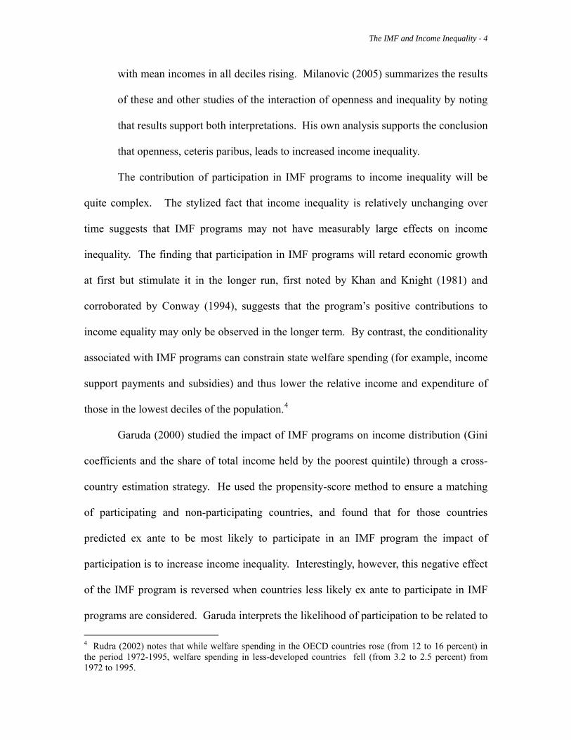
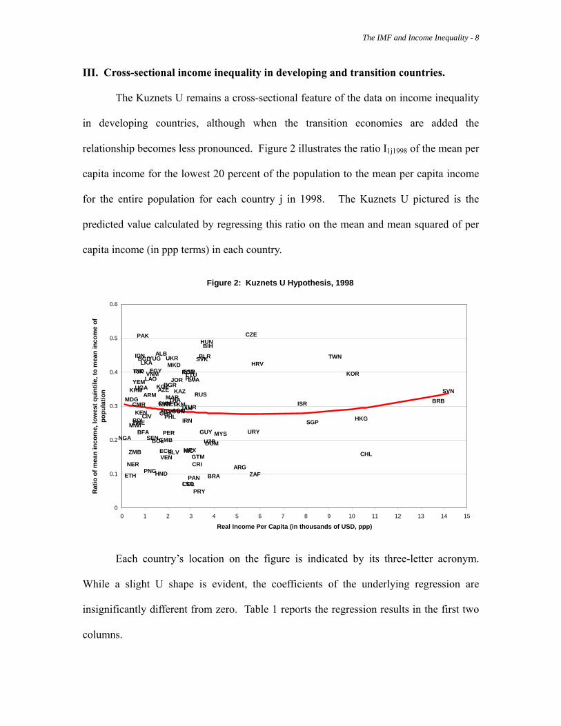
The Kuznets U remains a cross-sectional feature of the data on income inequality
in developing countries, although when the transition economies are added the
relationship becomes less pronounced. Figure 2 illustrates the ratio I1j1998 of the mean per
capita income for the lowest 20 percent of the population to the mean per capita income
for the entire population for each country j in 1998. The Kuznets U pictured is the
predicted value calculated by regressing this ratio on the mean and mean squared of per
capita income (in ppp terms) in each country.
Figure 2: Kuznets U Hypothesis, 1998
SVNBRB
CHL
HKG
KOR
TWN
SGP
ISR
HRV
ZAF
URY
CZE
ARG
MYS
BRA
DOMUZB
BIHHUN
GUY
BLRSVK
RUS
PRY
GTMCRI
PAN
LVAPOLLTU
TUR
MEXNIC
ESTROM
COLLSO
IRN
JAM
KAZ
TKMTUNAGO
JOR
THA
MKD
SLV
MAR
UKR
GEO
PHL
BGR
PER
MDA
VEN
GMB
GHA
ECU
MRTCHN
AZEKGZ
HND
ALB
BOL
EGY
YUG
SEN
VNMLAO
PNG
ARM
CIV
LKABGD
BFA
PAK
UGA
KEN
IDN
IND
YEM
CMR
ZWE
TJK
BDI
KHM
MWI
ZMB
NER
MDG
ETH
NGA
0
0.1
0.2
0.3
0.4
0.5
0.6
0 1 2 3 4 5 6 7 8 9 10 11 12 13 14 15
Real Income Per Capita (in thousands of USD, ppp)
Rat
io o
f mea
n in
com
e, lo
wes
t qui
ntile
, to
mea
n in
com
e of
po
pula
tion
Each country’s location on the figure is indicated by its three-letter acronym.
While a slight U shape is evident, the coefficients of the underlying regression are
insignificantly different from zero. Table 1 reports the regression results in the first two
columns.

The IMF and Income Inequality - 9
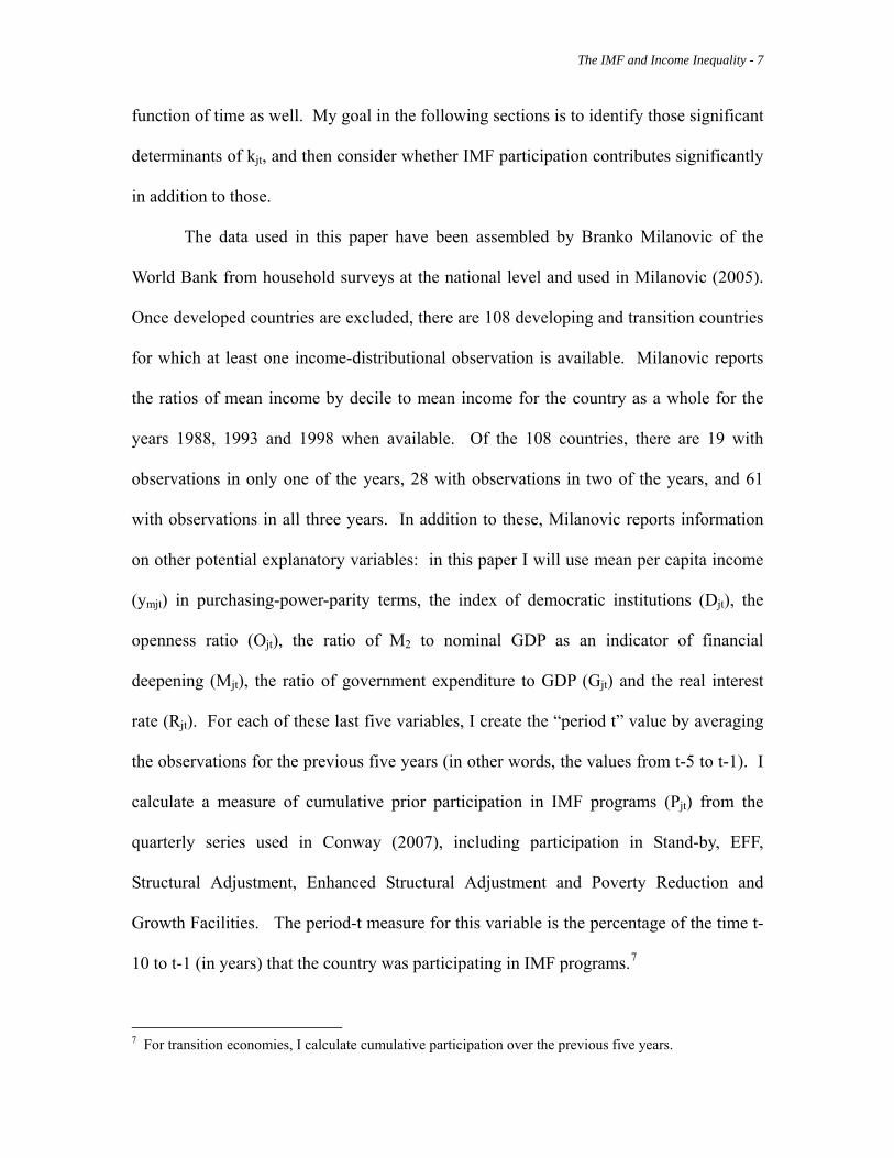
The transition economies tend to lessen the significance of this cross-sectional
relationship: they tend to have intermediate real income per capita and relatively high
mean income ratios. When the transition economies are excluded in 1998 there are 67
countries remaining; for those, the Kuznets U is significantly evident in the data. The
third and four columns in Table 1 report the results of that regression, while Figure 3
illustrates the derived Kuznets curve.
Figure 3: Kuznets' U Hypothesis, 1998, for developing countries alone
BRB
CHL
HKG
KOR
TWN
SGP
ISR
ZAF
URY
ARG
MYS
BRA
DOM
GUY
PRY
GTMCRI
PAN
MEXNIC
COLLSO
IRN
JAMTUNAGO
JOR
THA
SLV
MAR
PHL
PER
VEN
GMB
GHA
ECU
MRTCHN
HND
BOL
EGY
SEN
VNMLAO
PNG
CIV
LKABGD
BFA
PAK
UGA
KEN
IDN
IND
YEM
CMR
ZWEBDI
KHM
MWI
ZMB
NER
MDG
ETH
NGA
0
0.1
0.2
0.3
0.4
0.5
0.6
0 1 2 3 4 5 6 7 8 9 10 11 12 13 14
Mean PPP Income (in thousands of USD)
Rat
io o
f mea
n in
com
e of
low
est q
uint
ile to
mea
n in
com
e
While the Kuznets U hypothesis is the most famous of explanations for the
evolution of income inequality, the introduction noted a number of other potential
explanations: openness, financial deepening, democratic institutions, and the impact of
participation in IMF programs. While these have valid theoretical roots, they are in
practice quite different to distinguish among. There are two major difficulties in testing
these hypotheses in econometric work. The first difficulty is the high correlation among
The IMF and Income Inequality - 10
advances in these various dimensions. Table 2 illustrates the significant correlations (in
bold numbers) among measures for the alternative explanations considered by Milanovic
(2005). Four of the six, in particular, are significantly correlated with the measure of
mean income used in estimating the Kuznets U. The second difficulty is the less-than-
complete coverage for some of the empirical measures. There are 258 country/year
observations of income share of the lowest quintile in the data set, and complete coverage
is only possible with ymjt and Pjt. The openness indicator is only available for 86 percent
of the sample, and the financial-deepening indicator is only available for 60 percent of
the sample. Real interest rates and government expenditures indicators are available for
less than half, and when both are included only 1/3 of the sample can be used.
This is unfortunate, for the censoring involved with data availability is not
innocuous. Table 3 reports the means of the ymjt, Pjt and I1jt variables by availability of
explanatory variable. Those missing in each case will have participated less on average
in IMF programs than those for which we have data. Those missing in each case also
tend to have more equal income distributions than those for which data are available.
The countries with Demojt missing have larger mean income than those for which data
are available.
There will thus be a trade-off to keep in mind when adding these explanatory
variables with incomplete coverage – more complete hypothesis testing, but for a
censored sample.
It is unfortunately beyond the scope of this paper to decipher the common causes
of the movements in the explanatory variables.8 I will assume that the other explanatory
8 Rodrik et al. (2004) provides a nice econometric decomposition of the contributions of integration and institutional development to economic growth and concludes that “institutions rule”.
The IMF and Income Inequality - 11
variables have a potentially non-linear component determined by their level of
development, and that the real income per capita is a valid instrument for the level of
development. I use cross-country regressions in this sample to identify the component of
the variables due to shifts in level of development, and consider the residual from that
regression to be the non-development-component of the explanatory variable. 9 For
example, if the estimated equation is specified as:
Ojt = a + b* ymjt + c* (ymjt)2 + εOjt (4)
εOjt is then the openness indicator used in the regressions. Similar indicators are derived
for cumulative prior participation in IMF programs (εPjt), democratic institutions (εDjt)
and financial deepening (εMjt)
Table 4 reports the results of Kuznets regressions building upon Table 1 with the
addition of explanatory indicators as regressors. The first pair of regressions in Table 4 is
identical to those of Table 1: the left-hand side reports the results for all developing and
transition countries, while the right-hand side reports the results for developing countries
alone. When the indicator of cumulative prior IMF participation is added, the sign in
both sets of regressions is negative – increased prior IMF participation leads on average
to increased inequality. This effect is significant for the complete sample, but
insignificant for the developing countries alone.
When both IMF participation and country openness indicators are added, εOjt has
an insignificant coefficient in both sets of regressions – and 14 percent of the
observations (all from transition countries) are excluded. This has an important effect on 9 Those regressions are reported in the appendix Table A1.

The IMF and Income Inequality - 12
the Kuznets U coefficients, with the significant inverted-U shape of the preceding
regressions replaced with the expected (though insignificant) U shape. The impact of
IMF participation remains significant in the full sample, although smaller in magnitude
than in the preceding regression.
When the indicator for democratic institutions is added, the full sample shrinks
further to only 80 percent of the original size. The εDjt increases income inequality in
both samples by a comparable and significant amount. IMF participation and openness
are both insignificant in this sample. When financial deepening is added, the sample
shrinks still further -- to 56 percent of the original size. εMjt enters with positive sign and
significant coefficient: the greater financial depth of a developing or transition country,
the greater the equality of income. The coefficient on εDjt becomes insignificant, while
for the developing-country sample the openness indicator comes in with negative and
significant coefficient.
Correlation coefficients among the adjusted variables are reported in Table 5, and
these indicate the source of shifting significance and coefficient magnitude as regressors
are added.10 Even after removing the joint dependence on the level of development,
these explanatory variables remain highly correlated. Participation in IMF programs is
significantly and positively correlated with the degree of democratic institutions, and
significantly and negatively correlated with the degree of financial deepening. The more
democratic countries also tend to be significantly shallower financially than the less-
democratic countries in the sample.
10 When the correlation matrix is created for 1998 alone, the pattern and magnitude of correlation coefficients is quite similar. This indicates that the pattern observed here is due to cross-country variation rather than time-series variation.
The IMF and Income Inequality - 13
While we may not be able to state a priori the causal relationships between
institutional depth, financial depth and openness, we can postulate that participation in
IMF programs does not make a significant contribution to the pattern of income
inequality across developing countries at any point in time, and does not in transition plus
developing countries once other factors (financial depth, democratic institutions) are
introduced. In fact, if we expect participation in an IMF program to have an effect on
income distribution, we anticipate that its effect will be observed over time. I turn to that
possibility in the next section.
IV. Measuring the intertemporal impact of participation in IMF programs on
income inequality.
The derivation of the inequality ratio in equation (3) suggests that deviations in
this ratio will be largely due to cross-country differences in kj. That derivation of the
inequality ratio has no intertemporal component at all – a country j will remain with
constant I1jt in every t. In reality, the inequality coefficients are not constant. Figure 4
illustrates the empirical frequency of the percentage change in I1jt from the value five
years previously.11 While near-zero change is the modal outcome overall, there are
substantial numbers of observations with large percentage changes in this ratio. In this
section I investigate whether these changes can be attributed to participation in IMF
programs on average.
11 The graph points measure the number of observations falling in the range from 10 percentage points below to the point listed on the graph. For example, the observations at 0 represent all observations with values between -10 and 0.

The IMF and Income Inequality - 14
The dependent variable in this section is λ20jt = ΔI20jt/I20jt-1: the change in inequality ratio
in country j from period t-1 (five years previously) to period t. Considering percentage
changes should remove the development-level effects, and will also eliminate one
observation per country considered. Table 6 reports the results of Kuznets-like
regressions on λ20jt.
Figure 4: Distribution of changes in Inequality Ratio over Five Years
-5
0
5
10
15
20
25
30
35
-70 -60 -50 -40 -30 -20 -10 0 10 20 30 40 50 60 70 80 90 100
Percent change
Num
ber o
f obs
erva
tions
Total Sample 1993 1998
The initial panel in Table 6 reports the result of a regression of the percentage
change in the inequality ratio on the lagged mean and lagged mean squared of per capita
real income.12 The Kuznets U is evident in the percentage change as well; i.e., the
percentage change in the mean income of the lowest quintile relative to overall mean
income is initially declining as countries become more developed and then rises for the
most-developed countries in the sample. This pattern is evident in all specifications 12 For example: if the dependent variable is λ20k98, then it measures the percentage change from 1993 to 1998 in mean income of the lowest quintile in country k divided by the mean income for country k. The right-hand side variables are the real per capita income in 1993 in country k and that variable squared.
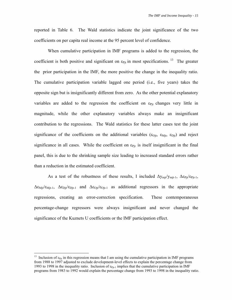
The IMF and Income Inequality - 15
reported in Table 6. The Wald statistics indicate the joint significance of the two
coefficients on per capita real income at the 95 percent level of confidence.
When cumulative participation in IMF programs is added to the regression, the
coefficient is both positive and significant on εPjt in most specifications. 13 The greater
the prior participation in the IMF, the more positive the change in the inequality ratio.
The cumulative participation variable lagged one period (i.e., five years) takes the
opposite sign but is insignificantly different from zero. As the other potential explanatory
variables are added to the regression the coefficient on εPjt changes very little in
magnitude, while the other explanatory variables always make an insignificant
contribution to the regressions. The Wald statistics for these latter cases test the joint
significance of the coefficients on the additional variables (εOjt, εMjt, εDjt) and reject
significance in all cases. While the coefficient on εPjt is itself insignificant in the final
panel, this is due to the shrinking sample size leading to increased standard errors rather
than a reduction in the estimated coefficient.
As a test of the robustness of these results, I included Δymjt/ymjt-1, ΔεPjt/εPjt-1,
ΔεMjt/εMjt-1, ΔεDjt/εDjt-1 and ΔεOjt/εOjt-1 as additional regressors in the appropriate
regressions, creating an error-correction specification. These contemporaneous
percentage-change regressors were always insignificant and never changed the
significance of the Kuznets U coefficients or the IMF participation effect.
13 Inclusion of εPjt in this regression means that I am using the cumulative participation in IMF programs from 1988 to 1997 adjusted to exclude development-level effects to explain the percentage change from 1993 to 1998 in the inequality ratio. Inclusion of εPjt-1 implies that the cumulative participation in IMF programs from 1983 to 1992 would explain the percentage change from 1993 to 1998 in the inequality ratio.

The IMF and Income Inequality - 16
V. Conclusions and extensions.
We can restate the initial hypothesis as follows: once other factors determining
income inequality are controlled for, is there an independent and significant effect of
participation in IMF programs on income inequality? Based on the evidence provided
here, I conclude that it will be difficult to attribute any of the cross-country differences in
income inequality to participation in IMF programs. However, there is a significant and
pro-equality effect of participation in IMF programs evident in the intertemporal
dimension of the data.
The problem in identifying the cross-country effects begins with the difficulty in
assigning causality among the potentially important variables, but does not end there.
Cross-country regressions like these are based upon the implicit assumption that the
process generating income inequality from the independent variables is identical across
countries. There are also, as Milanovic (2004) documents, significant differences across
countries in administration of household surveys and in calculation of income quantiles.
In the end, these results should be taken as suggestive; the rejection of the hypothesis that
participation in IMF programs is responsible for cross-country differences in income
inequality seems warranted, but will require more detailed work to be made definitive.
The significant impact of IMF programs on the time path of income inequality is
evident in these data, but it is important to recognize that for each country there are at
most two observations of differenced data. This is not a feature that allows confidence in
describing the time path of adjustments in income inequality due to participation in IMF
programs, Rather, I establish that on average the participation in IMF programs is
significantly associated with an adjustment toward greater income equality.

The IMF and Income Inequality - 17
This does not invalidate the complaint that IMF programs tend to reduce
government expenditure on goods targeted to the poor: those complaints may well be
true, since government expenditures of this type will in many cases not enter the
calculations of inequality based upon household surveys. This concern will be a useful
direction for further research.
This research design is predicated on the absence of sub-groups of countries with
strongly different experiences; if they exist, these sub-groups should be addressed
explicitly. I have begun this in the current paper by redoing the analysis with transition
economies excluded. Such an exclusion is natural, since the most important income-
distributional event during the data period was the end of the Soviet Union and the
relatively more unequal income distributions that followed. Given that the successor
states of the Soviet Union had both (a) strongly worsened income equality after
independence and (b) no prior participation in IMF programs, the positive effect of
participation on income equality could well be an artifact of that event. Redoing the
analysis for only the developing countries demonstrates that this was not a defining factor
in the results reported here, but more attention to such sub-groups will be useful in future
research.
Garuda (2000) serves as the benchmark for work relating IMF programs to
income inequality, but due to the difference in research design the results here are not
directly comparable. I can suggest one qualification to Garuda’s conclusions, and one
direction in which this paper should be extended. First, the qualification: Garuda’s result
that those more in need of IMF programs are more likely to lose from them is probably
an artifact of the cross-country dimension of income inequality. Here, the propensity to

The IMF and Income Inequality - 18
participate will be strongly correlated with developmental indicators, and the sorting
going on in that paper could simply be the sorting picked up by my developmental
regressors. Second, the extension: the participation variable Pjt in this paper could be
enhanced by considering the prior likelihood of participation. Once the analysis is
confined to the intertemporal dimension – one that Garuda (2000) did not consider – the
possibility remains that Garuda’s conclusions will be re-affirmed here.

The IMF and Income Inequality - 19
Table 1: Regression results, Kuznets U hypothesis All developing and transition
economies Excluding transition economies
Coefficient Std. Error Coefficient Std. Error Full Sample: Intercept 0.277 * 0.018 0.304 * 0.016 ym98 0.020 * 0.009 -0.027 * 0.009 (ym98)2 -0.0014 * 0.0007 0.0025 * 0.001 R2 0.02 0.05 F value 2.52 5.19 * Critical F(2,N-2) 3.02 3.03 N 258 186 1998: Intercept 0.304 * 0.028 0.317 * 0.027 ym98 -0.010 0.014 -0.043 * 0.015 (ym98)2 0.0009 0.001 0.004 * 0.001 R2 0.01 0.13 F value 0.45 4.80 * Critical F(2,N-2) 3.11 3.14 N 93 66 1993: Intercept 0.292 * 0.025 0.295 * 0.025 ym93 -0.002 0.013 -0.021 0.013 (ym93)2 0.0004 0.001 0.002 0.001 R2 0.004 0.02 F value 0.17 0.55 Critical F(2,N-2) 3.11 3.14 N 93 70 1988: Intercept 0.209 * 0.043 0.293 * 0.036 ym88 0.091 * 0.023 -0.011 0.022 (ym88)2 -0.007 * 0.002 0.002 0.002 R2 0.18 0.02 F value 7.83 * 0.51 Critical F(2,N-2) 3.13 3.18 N 72 47 * indicates significance at 95 degree level of confidence.

The IMF and Income Inequality - 20
Table 2: Pearson Correlations among independent variables ymjt Openjt M2jt/Yjt DFIjt/Yjt Demojt Govjt/Yjt Rintrjt
ymjt
Openjt 0.40 (223)
M2jt/Yjt 0.41 (153)
0.49 (152)
DFIjt/Yjt 0.14 (215)
0.56 (209)
-0.01 (147)
Demojt 0.33 (233)
0.03 (206)
-0.10 (147)
0.13 (201)
Govjt/Yjt 0.17 (111)
0.23 (110)
0.22 (109)
0.11 (108)
0.06 (109)
Rintrjt 0.10 (122)
-0.06 (122)
0.05 (122)
0.03 (120)
0.06 (117)
-0.00 (85)
CPjt -0.29 (258)
-0.20 (223)
-0.39 (153)
-0.03 (215)
0.12 (233)
-0.14 (111)
0.10 (122)
Numbers in parentheses are the number of observations used in calculating correlation. Statistics in bold are significantly different from zero at 95 percent level of confidence. Table 3: Means of Variables of Interest for Missing and non-missing Observations Number
missing I20jt CPjt ymjt
Missing Not missing
Missing Not missing
Missing Not missing
Openjt 35 0.48 0.29 0.02 0.36 2.86 2.75 Demojt 25 0.36 0.31 0.06 0.34 4.38 2.59 Govjt/Yjt 147 0.34 0.29 0.25 0.39 2.56 3.04 Rintrjt 136 0.35 0.27 0.20 0.43 2.56 3.00 M2jt/Yjt 105 0.35 0.29 0.18 0.39 2.50 2.95 Source: author’s calculation.

The IMF and Income Inequality - 21
Table 4: Independent Impact of Explanatory Variables All developing and transition
economies Excluding transition economies
Coefficient Std. Error Coefficient Std. Error Full Sample: Intercept 0.277 * 0.018 0.302 * 0.017 ymt 0.020 * 0.009 -0.027 * 0.009 (ymt)2 -0.0015 * 0.0008 0.0025 * 0.001 R2 0.02 0.05 F value 2.52 5.19 * Critical F(2,N-2) 3.02 3.03 N 258 183
Adding IMF participation: Intercept 0.277 * 0.018 0.302 * 0.027 ymt 0.020 * 0.009 -0.027 * 0.015 (ymt)2 -0.0014 * 0.0007 0.0025* 0.001 εPjt -0.114 * 0.028 -0.019 0.026 R2 0.08 0.06 F value 7.45 3.61 * Critical F(2,N-2) 3.02 3.03 N 258 183
Adding IMF participation and Openness: Intercept 0.299 * 0.017 0.302 * 0.016 ymt -0.006 0.009 -0.027 * 0.009 (ymt)2 0.0007 0.0007 0.0025 * 0.001 εPjt -0.055 * 0.027 -0.022 0.027 εOjt -0.026 0.016 -0.020 0.015 R2 0.03 0.07 F value 1.87 3.18 * Critical F(2,N-2) 3.02 3.03 N 223 183
(continued on following page)

The IMF and Income Inequality - 22
Table 4 continued: Adding IMF Participation, Openness and Democratic Institutions: Intercept 0.298 * 0.017 0.307 * 0.017 ymt -0.005 0.009 -0.032 * 0.009 (ymt)2 -0.0005 0.001 0.003 * 0.002 εPjt -0.045 0.028 -0.015 0.027 εOjt -0.024 0.017 -0.021 0.016 εDjt -0.007 * 0.002 -0.007 * 0.002 R2 0.06 0.12 F value 2.70 * 4.62 * Critical F(2,N-2) N 206 171
Adding IMF Participation, Openness, Democratic Institutions and Financial Deepening: Intercept 0.303 * 0.023 0.327 * 0.019 ymt -0.008 0.012 -0.049 * 0.010 (ymt)2 0.001 0.001 0.004 * 0.001 εPjt -0.026 0.036 0.035 0.031 εOjt -0.048 0.030 -0.099 * 0.026 εDjt -0.005 0.003 -0.003 0.002 εMjt 0.072 * 0.035 0.121 * 0.033 R2 0.09 0.28 F value 2.35 7.16 * Critical F(2,N-2) N 146 119 Source: author’s calculations. GMM estimation
Table 5: Pearson Correlations among adjusted variables εPjt εOjt εDjt εMjt
εPjt 1.00 (258)
εOjt -0.07 (223)
1.00 (223)
εDjt 0.24 (233)
-0.11 (206)
1.00 (233)
εMjt -0.28 (153)
0.38 (152)
-0.23 (147)
1.00 (153)
Numbers in parentheses are the number of observations used in calculating correlation. Statistics in bold are significantly different from zero at 95 percent level of confidence.

The IMF and Income Inequality - 23
Table 6: Intertemporal Impact of Explanatory Variables on λ20jt
All developing and transition economies
Excluding transition economies
Coefficient Std. Error Coefficient Std. Error Full Sample: Intercept 0.090 0.049 0.056 0.057 ymt-1 -0.084 * 0.022 -0.057 0.033 (ymt-1)2 0.007 * 0.002 0.005 0.003 R2 0.07 0.03 Wald 18.8 * 10.41 * N 150 102
Adding IMF participation: Intercept 0.043 0.050 0.016 0.058 ymt-1 -0.076 * 0.022 -0.051 * 0.023 (ymt-1)2 0.007 * 0.002 0.005 * 0.002 εPjt 0.298 * 0.102 0.270 * 0.135 εPjt-1 -0.118 0.101 -0.128 0.123 R2 0.12 0.07 Wald 9.24 * 4.01 N 150 102
Adding IMF participation and Openness: Intercept 0.008 0.055 0.015 0.058 ymt-1 -0.049 * 0.024 -0.051 * 0.024 (ymt-1)2 0.005 * 0.002 0.005 * 0.002 εPjt 0.260 * 0.114 0.271 * 0.134 εPjt-1 -0.113 0.106 -0.129 0.124 εOjt 0.100 0.108 0.007 0.137 εOjt-1 -0.107 0.101 -0.007 0.128 R2 0.07 0.07 Wald 1.20 0.00 N 117 102
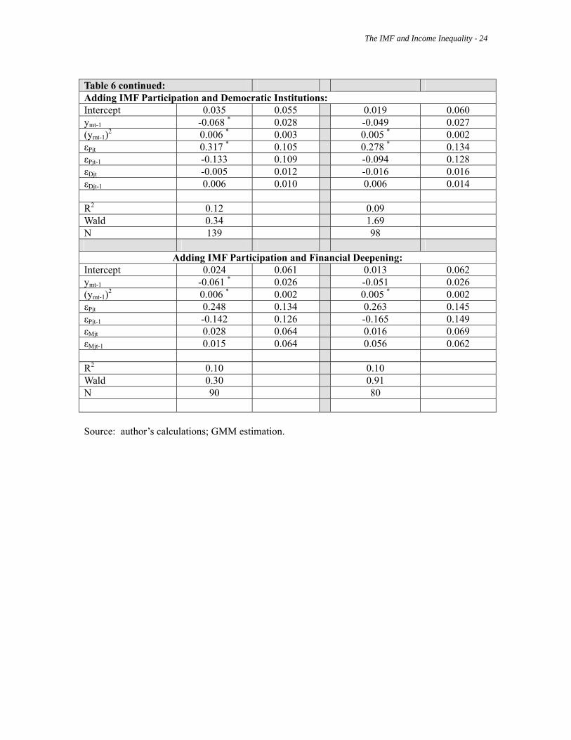
The IMF and Income Inequality - 24
Table 6 continued: Adding IMF Participation and Democratic Institutions: Intercept 0.035 0.055 0.019 0.060 ymt-1 -0.068 * 0.028 -0.049 0.027 (ymt-1)2 0.006 * 0.003 0.005 * 0.002 εPjt 0.317 * 0.105 0.278 * 0.134 εPjt-1 -0.133 0.109 -0.094 0.128 εDjt -0.005 0.012 -0.016 0.016 εDjt-1 0.006 0.010 0.006 0.014 R2 0.12 0.09 Wald 0.34 1.69 N 139 98
Adding IMF Participation and Financial Deepening: Intercept 0.024 0.061 0.013 0.062 ymt-1 -0.061 * 0.026 -0.051 0.026 (ymt-1)2 0.006 * 0.002 0.005 * 0.002 εPjt 0.248 0.134 0.263 0.145 εPjt-1 -0.142 0.126 -0.165 0.149 εMjt 0.028 0.064 0.016 0.069 εMjt-1 0.015 0.064 0.056 0.062 R2 0.10 0.10 Wald 0.30 0.91 N 90 80 Source: author’s calculations; GMM estimation.
The IMF and Income Inequality - 25
Bibliography Conway, P.: “IMF Lending Programs: Participation and Impact”, Journal of
Development Economics 45, 1994, pp. 365-391. Conway, P.: “The Revolving Door: Duration and Recidivism in IMF Programs”, Review
of Economics and Statistics, 2007 (forthcoming). Deininger, K. and L. Squire: “New Ways of Looking at Old Issues: Inequality and
Growth”, Journal of Development Economics 57, 1998, pp. 259-287. Dollar, D. and A. Kraay: “Growth is Good for the Poor”, Journal of Economic Growth
7/3, 2002, pp. 195-225. Garuda, G.: AThe Distributional Effect of IMF Programs: A Cross-Country Analysis@,
World Development 28/6, 2000, pp. 1031-1051. Khan, M. and M. Knight: “Stabilization Programs in Developing Countries: A Formal
Framework”, IMF Staff Papers 28, 1981, pp. 1-53. Kuznets, S.: “Economic Growth and Income Inequality”, American Economic Review
45, 1955, pp. 1-28. Kuznets, S.: Modern Economic Growth. New Haven, CT: Yale University Press, 1966. Li, H., L. Squire and H. Zou: “Explaining International and Intertemporal Variations in
Income Inequality”, Economic Journal 108, 1998, pp. 26-43. Milanovic, B.: Worlds Apart: Global and International Inequality 1950-2000. Princeton,
NJ: Princeton University Press, 2004. Milanovic, B.: “Can We Discern the Effect of Globalization on Income Distribution?
Evidence from Household Surveys”, World Bank Economic Review 19/1, 2005, pp. 21-44.
Ravallion, M.: “Growth, Inequality and Poverty: Looking Beyond Averages”, World
Development 29/11, 2001, pp. 1803-1815. Rodrik, D., A. Subramanian and F. Trebbi: “Institutions Rule: The Primacy of
Institutions over Geography and Integration in Economic Development”, Journal of Economic Growth 9/2, June 2004.
Rudra, N.: “Globalization and the Decline of the Welfare State in Less Developed
Countries”, International Organization 56/2, 2002.