participating simulation modules -...

1

Description of broadband ground

motion simulation methods

Paul Somerville, URS

Participating Simulation Modules

GREENS FUNCTION BASED MODULES

• SDSU – Olsen/Mai – operational • UCSB – Archuleta et al – operational • URS – Graves/Pitarka – operational

• Irikura – asperity source model – to be implemented • Zeng/Anderson – to be implemented NON-GREENS FUNCTION BASED MODULES • Point source stochastic model – Boore - to be implemented • Finite-fault stochastic model – Atkinson - to be implemented

GMPE • Empirical GMPE with event terms - to be implemented

2

Simulation Methods Described:

1. URS 2. UCSB 3. SDSU 4. Irikura 5. Zeng/Anderson

1.  URS Hybrid Approach to Broadband Ground Motion Simulations

(Graves and Pitarka, 2004)

3

For f < 1 Hz: •  Kinematic representation of heterogeneous rupture on a

finite fault –  Slip amplitude and rake, rupture time, slip function

•  1D FK or 3D FDM approach for Green’s function

For f > 1 Hz: •  Extension of Boore (1983) with limited kinematic

representation of heterogeneous fault rupture –  Slip amplitude, rupture time, conic averaged radiation pattern,

Stochastic phase •  Simplified Green’s functions for 1D velocity structure

–  Geometrical spreading, impedance effects Both frequency ranges have the nonlinear site amplification based

on Vs30 (Campbell and Bozorgnia, 2008)

Scenario Earthquake

•  Begin with uniform slip having mild taper at edges.

•  Use Mai and Beroza (2002) spatial correlation functions (Mw dependent, K-2 falloff) with random phasing to specify entire wavenumber spectrum.

Kinematic Rupture Generator – Unified scaling rules for rise time, rupture speed and corner frequency – Depth scaling for shallow (< 5 km) moment release: rise time (increase) and rupture speed (decrease)

4

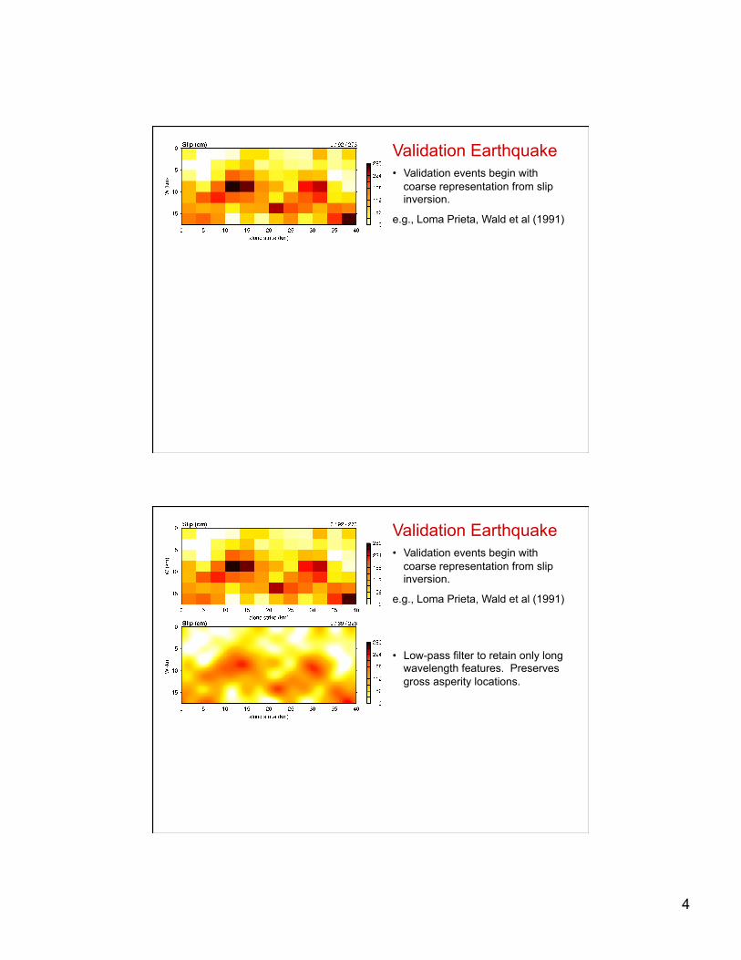
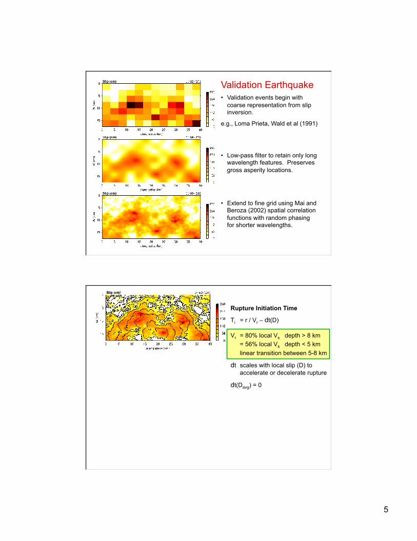
Validation Earthquake •  Validation events begin with

coarse representation from slip inversion.

e.g., Loma Prieta, Wald et al (1991)




•  Low-pass filter to retain only long wavelength features. Preserves gross asperity locations.

5

•  Low-pass filter to retain only long wavelength features. Preserves gross asperity locations.




•  Extend to fine grid using Mai and Beroza (2002) spatial correlation functions with random phasing for shorter wavelengths.

Rupture Initiation Time

Ti = r / Vr – dt(D)

Vr = 80% local Vs depth > 8 km = 56% local Vs depth < 5 km linear transition between 5-8 km

dt scales with local slip (D) to accelerate or decelerate rupture

dt(Davg) = 0

6

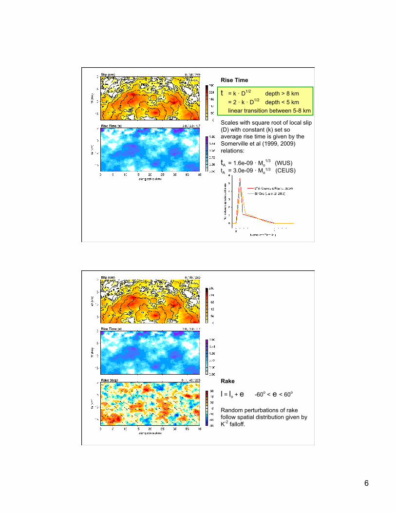
Rise Time

t = k · D1/2 depth > 8 km = 2 · k · D1/2 depth < 5 km linear transition between 5-8 km

Scales with square root of local slip (D) with constant (k) set so average rise time is given by the Somerville et al (1999, 2009) relations:

tA = 1.6e-09 · Mo1/3 (WUS)

tA = 3.0e-09 · Mo1/3 (CEUS)

Rake

l = lo + e -60o < e < 60o

Random perturbations of rake follow spatial distribution given by K-2 falloff.

7

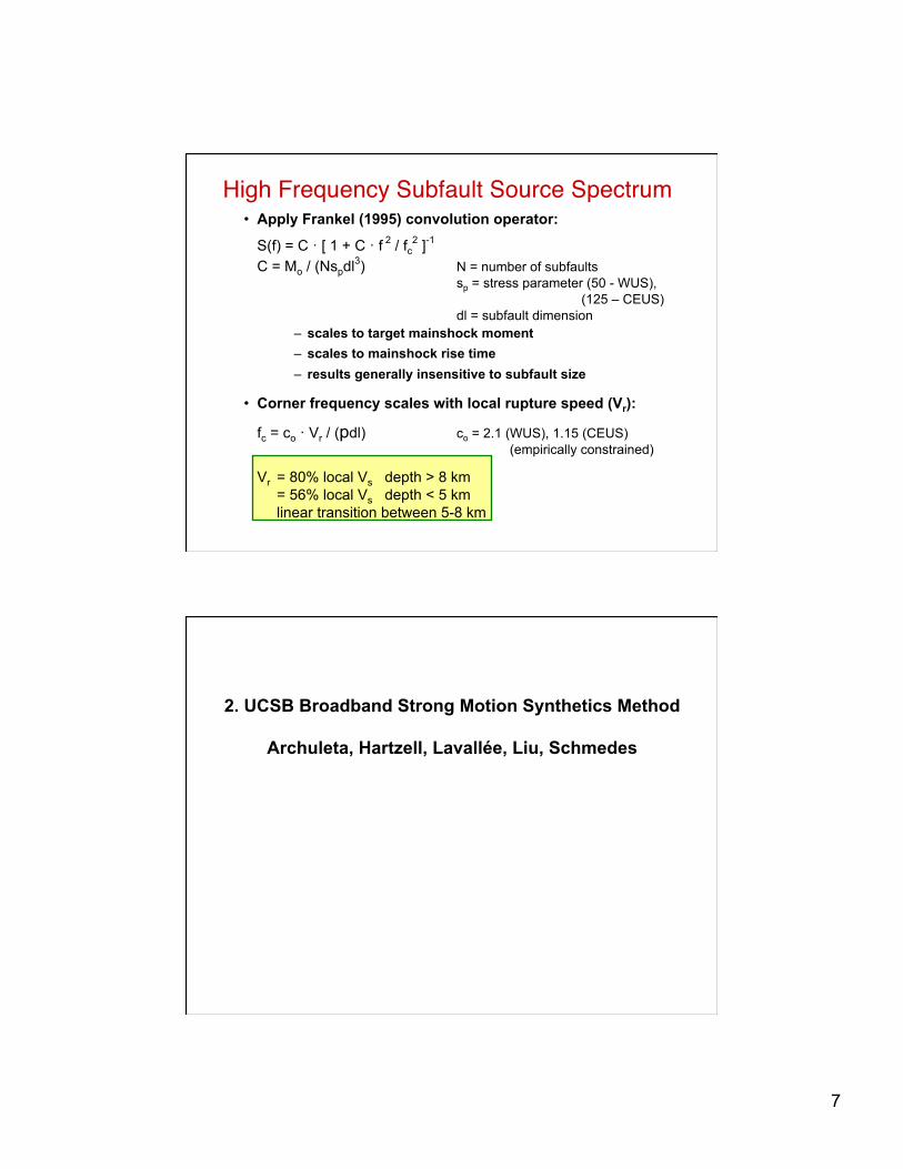
•  Corner frequency scales with local rupture speed (Vr):

fc = co · Vr / (pdl) co = 2.1 (WUS), 1.15 (CEUS) (empirically constrained)

Vr = 80% local Vs depth > 8 km = 56% local Vs depth < 5 km linear transition between 5-8 km

High Frequency Subfault Source Spectrum"•  Apply Frankel (1995) convolution operator:

S(f) = C · [ 1 + C · f 2 / fc2 ]-1

C = Mo / (Nspdl3) N = number of subfaults sp = stress parameter (50 - WUS), (125 – CEUS) dl = subfault dimension

–  scales to target mainshock moment –  scales to mainshock rise time –  results generally insensitive to subfault size

2. UCSB Broadband Strong Motion Synthetics Method

Archuleta, Hartzell, Lavallée, Liu, Schmedes

Liu, P., R. J. Archuleta and S. H. Hartzell (2006). Prediction of broadband ground-motion time histories: Hybrid low/high-frequency method with correlated random source parameters, Bull. Seismol. Soc. Am. vol. 96, No. 6, pp. 2118-2130, doi: 10.1785/0120060036. Schmedes, J., R. J. Archuleta, and D. Lavallée (2010). Correlation of earthquake source parameters inferred from dynamic rupture simulations, J. Geophys. Res., 115, B03304, doi:10.1029/2009JB006689.

8

Flowchart for Generating Broadband Strong Motion Synthetics

Liu, Archuleta, Hartzell, BSSA

Correlated Source Parameters (LAH)

Slip

Average rupture velocity

Rise time

Spatial correlation 30%

Spatial correlation 60%

(Liu, Archuleta, Hartzell, 2006)

9

New Kinematic Model (SAL) Schmedes, J., R. J. Archuleta, and D. Lavallée (2010), Correlation of earthquake source parameters inferred from dynamic rupture simulations, J. Geophys. Res., 115, B03304, doi:10.1029/2009JB006689.

Frequency dependent perturbation of strike, dip and rake (Pitarka et al, 2000)

With f1=1.0 Hz, f2=3.0 Hz

High Frequencies

Randomness of the high frequencies is generated in the source description.

€

ϕi =

ϕ0 f ≤ f1ϕ0 + ( f − f1) / f2 − f1)((2ri −1)ϕp , f1 < f < f2

ϕ0 + (2* ri −1)*ϕ p f2 ≤ f

⎧

⎨ ⎪

⎩ ⎪

(

10

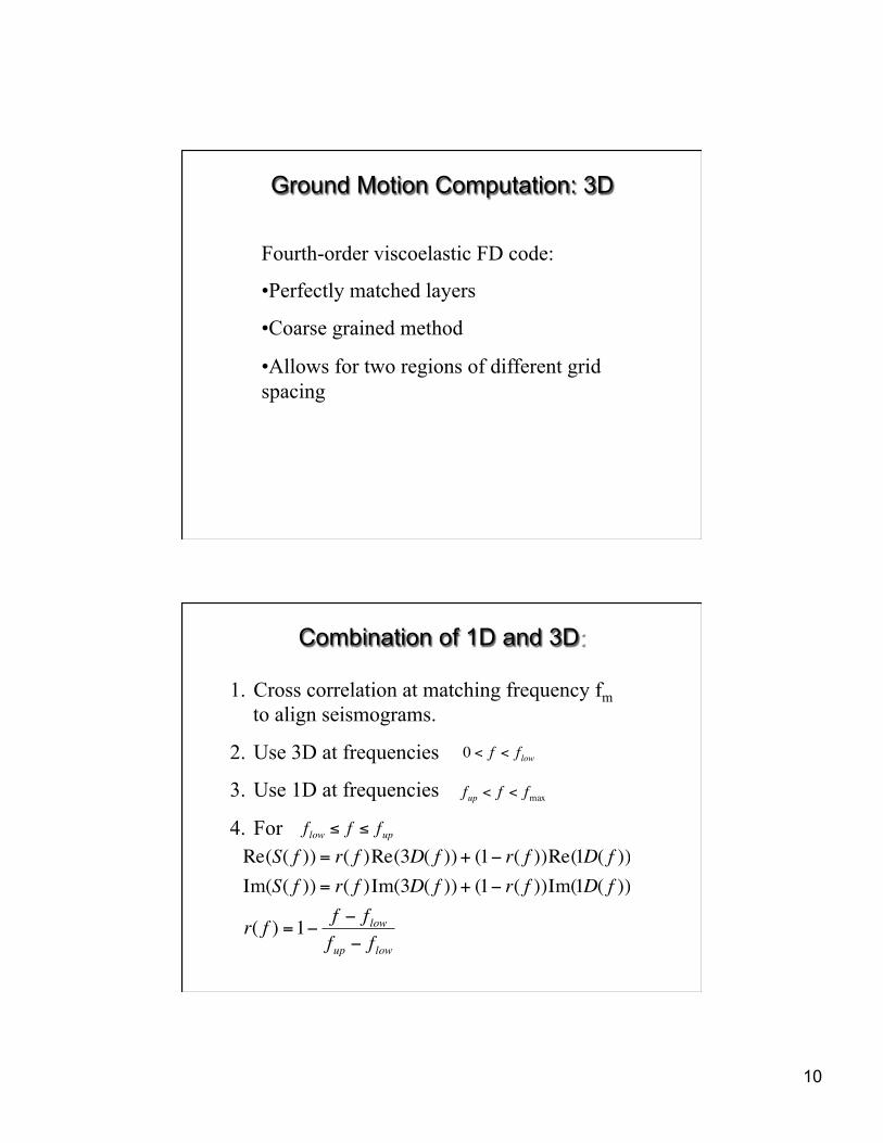
Ground Motion Computation: 3D

Fourth-order viscoelastic FD code:

• Perfectly matched layers

• Coarse grained method

• Allows for two regions of different grid spacing

Combination of 1D and 3D:

1.  Cross correlation at matching frequency fm to align seismograms.

2.  Use 3D at frequencies

3.  Use 1D at frequencies 4.  For

€

Re(S( f )) = r( f )Re(3D( f ))+ (1− r( f ))Re(1D( f ))Im(S( f )) = r( f )Im(3D( f ))+ (1− r( f ))Im(1D( f ))

r( f ) =1− f − f lowfup − f low

€

flow ≤ f ≤ fup€

0 < f < flow

€

fup < f < fmax

11

Martin Mai, Walter Imperatori, and Kim Olsen

Mai, P.M., W. Imperatori, and K.B. Olsen (2010). Hybrid broadband ground-motion simulations: combining long-period deterministic synthetics with high-frequency multiple S-to-S back-scattering, Bull. Seis. Soc. Am. 100, 5A, 2124-2142. Mena, B., P.M. Mai, K.B. Olsen, M.D. Purvance, and J.N. Brune (2010). Hybrid broadband ground motion simulation using scattering Green's functions: application to large magnitude events, Bull. Seis. Soc. Am. 100, 5A, 2143-2162.

3. Hybrid Broadband Ground-Motion Simulations: Combining Long-Period

Deterministic Synthetics with High-Frequency Multiple S-to-S Backscattering

Combines low-frequency deterministic synthetics (f ~ 1 Hz) with high-frequency scattering operators

Site effects: •  Soil structure •  (De-)amplification of ground motions •  Non-linear soil behavior

Scattering effects: •  inhomogeneities in Earth structure at all scales •  scattering model, based on site-kappa, Q, scattering and intrinsic attenuation, ηs and ηi

12

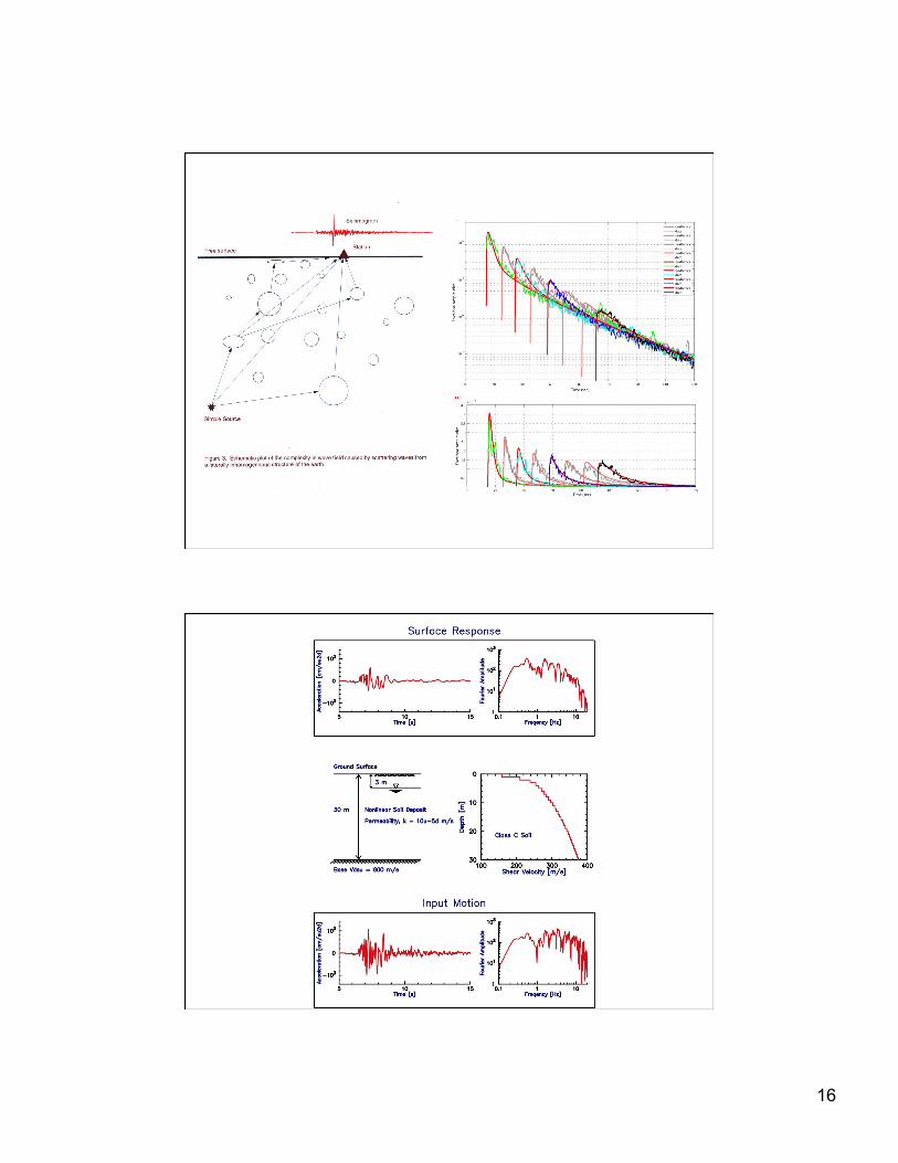
of the HF content of the seismic wave field based on multipleS-to-S backscattering theory. It is important to note that theconvolution with the STF also ensures the appropriate spec-tral properties of the scatterograms. While the scatteringGreen’s function exhibits a white noise spectrum, the veloc-ity spectrum of the scatterogram obtains a 1=f decay throughthe STF convolution operator. This spectral behavior of theHF scatterogram is needed for rendering it suitable to com-pute hybrid broadband seismograms. Figure 1 displays anexample of the scattering Green’s function (Fig. 1a), thescatterogram after convolving the scattering Green’s functionwith an appropriate STF (Fig. 1b) and the correspondingamplitude spectrum (Fig. 1c).

Combining Low-Frequency andHigh-Frequency Seismograms

Several methods have been proposed for combining HFand LF seismograms to compute hybrid broadband ground-

motions (Irikura and Kamae, 1994; Hartzell et al., 1999;Berge et al., 1998; Graves and Pitarka, 2004; Pulido andKubo, 2004; Liu et al., 2006). These techniques use differentparameterizations for the earthquake rupture process, forcomputing the LF and HF wave field, and for combiningthe two sets of seismograms. The latter step can be carriedout either in the time domain (e.g., Berge et al., 1998; Gravesand Pitarka, 2004) under consideration of the appropriateamplitude-scaling of the two time series or in the frequencydomain (Hartzell et al., 1999; Pulido and Kubo, 2004) byapplying a pair of matched filters. In almost all cases, theHF wave field is computed as a stochastic time series follow-ing the approach of Boore (1983), with fixed matching fre-quency near 1 Hz, based on the seismological observationthat source radiation and wave-propagation effects tend tobecome random at frequencies above f! 1 Hz (e.g., Pulidoand Kubo, 2004). However, the transition from the theoreti-cal radiation pattern of a double-couple source to isotropicradiation may not be abrupt. Based on observational

0 10 20 30 40-0.1

-0.05

0

0.05

0.1scattering Green’s function

Acc

lera

tion

(cm

/s2 )

Time (s)

0 10 20 30 40

-0.5

0

0.5

... convolved with STFVe

loci

ty (m

/s)

Time (s)

0.1 1.0 10.010-4

10-3

10-2

10-1

100amplitude spectra

Frequency (Hz)

convscat

0 20 40 60

!60

!40

!20

0

20

Time (s)

Velo

city

(cm

/s)

BBFDSC

0.1 1.0 10.0

0.1

1.0

10

Frequency (Hz)

Am

plitu

de (c

m/s

/Hz)

Am

plitu

de (c

m/s

/Hz)

BBFDSC

hybrid broadband seismogram composition

1/f

1/f

(a) (b) (c)

(d) (e)

Figure 1. Computation of hybrid broadband seismograms using scattering Green’s functions. (a) Site-specific scattering Green’s functionfor a point-source at the hypocenter; (b) scatterogram, formed by convolving the scattering Green’s function in (a) with a source-time function(STF) representing the temporal rupture evolution. (c) Fourier amplitude spectra for the time series in (a) and (b); the velocity-scatterogramdecays as 1=f (dotted line) beyond the corner frequency; (d) broadband seismogram (top) computed by combining the LF seismogram(center) with the site-specific HF scatterogram (bottom) using a Fourier-domain amplitude-and-phase matching technique (Mai and Beroza,2003). (e) Amplitude spectra for the time series in (d); the spectra of the broadband synthetics represent the LF motions at low frequencies(except for a small shift at the lowest frequency due to filtering of the LF synthetics) and the HF-scattering contribution at high frequencies(matching frequency and search range shown by vertical lines).

2128 P. M. Mai, W. Imperatori, and K. B. Olsen

Ø Scattering Green’s functions computed for each component of motion based on Zeng et al. (1991, 1993) and and P and S arrivals from 3D ray tracing (Hole, 1992) convolved with a dynamically-consistent source-time function, generating 1/f spectral decay

Ø Site-Scattering parameters (scattering and attenuation coefficient, site kappa, intrinsic attenuation) are taken from the literature and are partly based on the site-specific velocity structure.

Ø Assuming scattering operators and moment release originate throughout the fault, but starts at the hypocenter

Site-Specific Scattering Functions

Ø Hybrid broadband seismograms are calculated from low-frequency and high-frequency synthetics in the frequency domain using a simultaneous amplitude and phase matching algorithm (Mai and Beroza, 2003)

Example BB calculation

BB

SC

LF

BB = broadband LF = low frequency SC = scattering functions

1/f

Generation of hybrid broadband seismograms

13

4. Irikura Recipe

Miyake et al. (2003)

Irikura Recipe Parameters

Inner Fault Parameters "   Combined area of asperities Sa from the empirical relations of S-Sa

or Mo-Ao. "   Stress drop on asperities Δσa based on the multiple asperity model. "   Number of asperities from fault segments. "   Average slip of asperities Da from dynamic simulations. "   Effective stress for asperities σa and background area σb are given. "   Slip velocity time function given as Kostrov-like function.

Outer Fault Parameters "   Rupture area S is given. "   Seismic moment Mo from the empirical relation of Mo-S. "   Average static stress-drop Δσc from appropriate physical model

(e.g., circular crack model, tectonic loading model, etc.)

Extra Fault Parameters "   Rupture nucleation and termination are related to fault geometry.

Irikura and Miyake (2001, 2011)

14

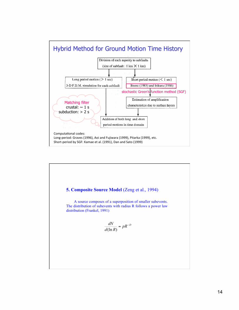
Hybrid Method for Ground Motion Time History

Matching filter crustal: ~ 1 s

subduction: > 2 s

Computa(onal codes: Long-‐period: Graves (1996), Aoi and Fujiwara (1999), Pitarka (1999), etc. Short-‐period by SGF: Kamae et al. (1991), Dan and Sato (1999)

stochastic Green’s function method (SGF)

5. Composite Source Model (Zeng et al., 1994)

A source composes of a superposition of smaller subevents. The distribution of subevents with radius R follows a power law distribution (Frankel, 1991)

DpRRd

dN −=)(ln

17

•  URS and Zeng’s models have considered scaling of rise-time/stress-drop and rupture speed for the upper 5 km depth.

•  URS, UCSB, Zeng, and SDSU have variable rupture velocities, subevent rakes, rise-time ~ local slip, K-2 fall off in slip distribution

•  UCSB considers dynamic rupture characteristics for slip time function, correlations between rupture speed, rise time, local slip, …

•  Irikura recipe uses a deterministic asperity source in place of K-2

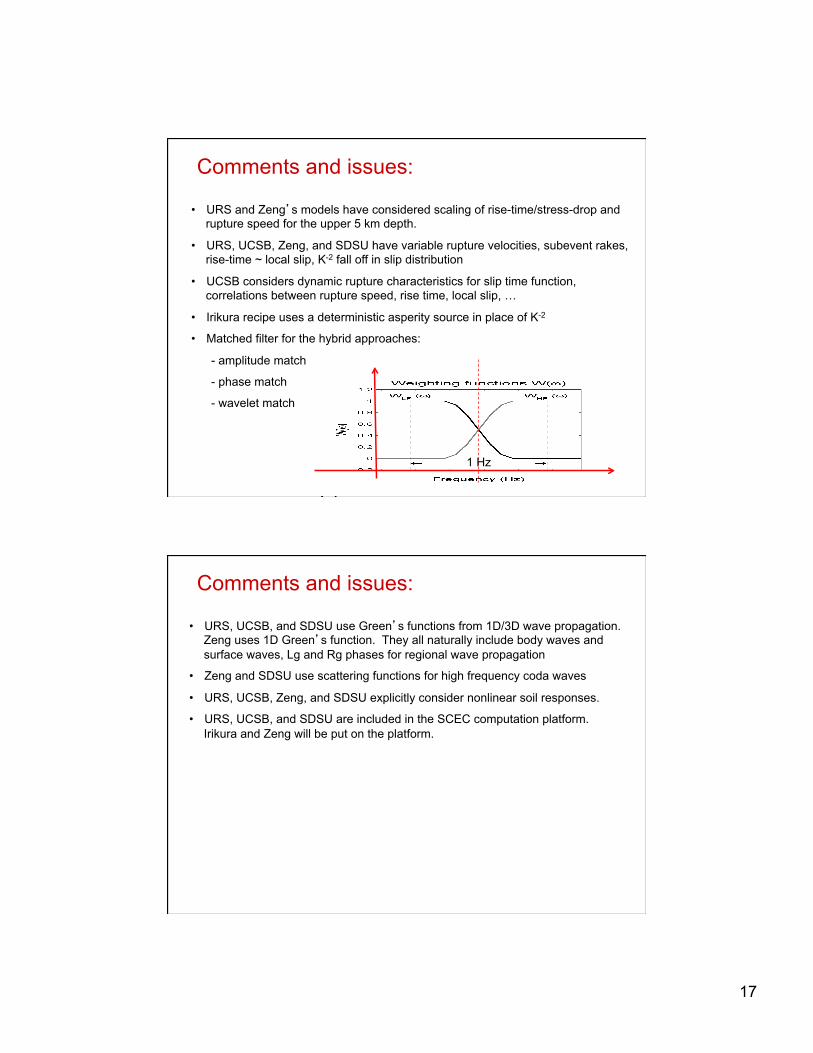
•  Matched filter for the hybrid approaches:

- amplitude match

- phase match

- wavelet match

Comments and issues:

1 Hz

•  URS, UCSB, and SDSU use Green’s functions from 1D/3D wave propagation. Zeng uses 1D Green’s function. They all naturally include body waves and surface waves, Lg and Rg phases for regional wave propagation

•  Zeng and SDSU use scattering functions for high frequency coda waves

•  URS, UCSB, Zeng, and SDSU explicitly consider nonlinear soil responses.

•  URS, UCSB, and SDSU are included in the SCEC computation platform. Irikura and Zeng will be put on the platform.

Comments and issues:

18

Input: For all the models: Fault geometry, hypocenter, P- and S-wave velocities, Qp and Qs, fmax, seismic moment, site condition based on Vs30 (nonlinearity), site kappa For URS, UCSB, Olsen, Zeng (except slip): Slip, rise-time, and rupture-time distribution; correlation between these source parameters Variable rake, strike, … For Irikura: deterministic asperity model In Zeng’s model: slip distribution is defined by subevent stress-drop with random distribution on subevent locations

participating simulation modules -...

Documents