partial differential equations - wordpress.com · 2017-10-07 · chapter 1 introduction a partial...
TRANSCRIPT


ii
Contents
Notations v
1 Introduction 1
1.1 History of PDE . . . . . . . . . . . . . . . . . . . . . . . . . . 21.2 Continuity Equation . . . . . . . . . . . . . . . . . . . . . . . 41.3 Definition and Well-Posedness of PDE . . . . . . . . . . . . . 61.4 Classification of PDE . . . . . . . . . . . . . . . . . . . . . . . 7
1.4.1 Classification of Second order Linear PDE . . . . . . . 71.4.2 Standard or Canonical Forms of Second Order PDE . . 81.4.3 Reduction to Standard Form . . . . . . . . . . . . . . . 91.4.4 Classification of Second Order Quasi-Linear . . . . . . 9
2 First Order PDE 13
2.1 Linear Transport Equation . . . . . . . . . . . . . . . . . . . . 132.2 Integral Surfaces and Monge Cone . . . . . . . . . . . . . . . . 152.3 Cauchy Problem . . . . . . . . . . . . . . . . . . . . . . . . . 162.4 Method of Characteristics . . . . . . . . . . . . . . . . . . . . 17
2.4.1 Examples . . . . . . . . . . . . . . . . . . . . . . . . . 192.5 Complete Integrals and General Solutions . . . . . . . . . . . 22
3 Second Order PDE 23
3.1 The Laplacian . . . . . . . . . . . . . . . . . . . . . . . . . . . 233.1.1 Laplacian in Different Coordinate Systems . . . . . . . 233.1.2 Harmonic Functions . . . . . . . . . . . . . . . . . . . 24
3.2 Poisson Equation in Rn . . . . . . . . . . . . . . . . . . . . . . 33
3.2.1 Fundamental Solution of Laplacian . . . . . . . . . . . 343.2.2 Solving Poisson Equation . . . . . . . . . . . . . . . . . 37
3.3 Dirichlet Problem . . . . . . . . . . . . . . . . . . . . . . . . . 40
iii

CONTENTS iv
3.3.1 Green’s Function . . . . . . . . . . . . . . . . . . . . . 413.3.2 Green’s Function for half-space . . . . . . . . . . . . . 463.3.3 Green’s Function for a disk . . . . . . . . . . . . . . . . 483.3.4 Dirichlet principle . . . . . . . . . . . . . . . . . . . . . 50
3.4 Neumann Problem . . . . . . . . . . . . . . . . . . . . . . . . 523.5 Heat Equation . . . . . . . . . . . . . . . . . . . . . . . . . . . 52
3.5.1 Fundamental Solution . . . . . . . . . . . . . . . . . . 533.5.2 Duhamel’s Principle . . . . . . . . . . . . . . . . . . . 53
3.6 Wave Equation . . . . . . . . . . . . . . . . . . . . . . . . . . 533.6.1 D’Alembert’s Formula . . . . . . . . . . . . . . . . . . 533.6.2 Method of Descent . . . . . . . . . . . . . . . . . . . . 533.6.3 Duhamel’s Principle . . . . . . . . . . . . . . . . . . . 53
Appendices 55
A The Gamma Function 57
B Surface Area and Volume of Disk in Rn 59
C Divergence Theorem 63
D Mollifiers and Convolution 65
Index 67

Notations
Symbols
∆∑n
i=1∂2
∂x2i
∇(
∂∂x1, . . . ∂
∂xn
)
.
Ω denotes an open subset of Rn, not necessarily bounded
∂Ω denotes the boundary of Ω
Rn denotes the n-dimensional Euclidean space
Dα ∂α1
∂x1α1. . . ∂αn
∂xnαn and α = (α1, . . . , αn)
Function Spaces
C(Ω) is the class of all continuous functions on Ω
Ck(Ω) is the class of all k-times (k ≥ 1) continuously differentiable functionson Ω
C∞(Ω) is the class of all infinitely differentiable functions on Ω
C∞c (Ω) is the class of all infinitely differentiable functions on Ω with compact
support
General Conventions
Br(x) denotes the open disk with centre at x and radius r
Sr(x) denotes the circle or sphere with centre at x and radius r
wn denotes the surface area of a n-dimensional sphere of radius 1.
v

NOTATIONS vi

Chapter 1
Introduction
A partial differential equation (PDE) is an equation involving an unknownfunction u of two or more variables and some or all of its partial derivatives.
Let Ω be an open subset of Rn and let u : Ω → R be a given function. Wedenote the partial derivative of u along ei = (0, 0, . . . , 1, 0, . . . , 0), the i-thcoordinate vector of Rn, as
uxi=
∂u
∂xi(x) = lim
h→0
u(x+ hei)− u(x)
h,
provided the limit exists. Similarly, one can consider higher order derivatives,as well. We now introduce Schwartz’s multi-index notation for derivative,which will be used to denote a PDE in a concise form. Let α = (α1, . . . , αn)be an n-tuple of non-negative integers and let |α| = α1+ . . .+αn. The partialdifferential operator of order α is denoted as,
Dα =∂α1
∂x1α1. . .
∂αn
∂xnαn=
∂|α|
∂x1α1 . . . ∂xnαn.
If α and β are two multi-indices, then α ≤ β means αi ≤ βi for all 1 ≤ i ≤ n.Also, α ± β = (α1 ± β1, . . . , αn ± βn), α! = α1! . . . αn! and x
α = xα11 . . . xαn
n .For k ≥ 1, we define Dku(x) := Dαu(x) | |α| = k. Thus, for k = 1, weregard Du as being arranged in a vector, i.e.,
Du = (ux1 , . . . uxn) .
We call this the gradient vector denoted as,
∇ :=
(
∂
∂x1, . . .
∂
∂xn
)
.
1

CHAPTER 1. INTRODUCTION 2
Similarly, for k = 2, we regard D2 as being arranged in a matrix form (calledthe Hessian matrix),
D2 =
∂2
∂x21
. . . ∂2
∂x1∂xn
∂2
∂x2∂x1. . . ∂2
∂x2∂xn
. . .∂2
∂xn∂x1. . . ∂2
∂x2n
n×n
.
The trace of the Hessian matrix is called the Laplace operator, denoted as∆ :=
∑ni=1
∂2
∂x2i. Note that under the order introduced on multi-indices α,
Dku(x) can be regarded as a vector in Rnk.
1.1 History of PDE
The study of partial differential equations started as a tool to analyse themodels of physical science. The PDE’s usually arise from the physical lawssuch as balancing forces (Newton’s law), momentum, conservation laws etc.The first PDE was introduced in 1752 by d’Alembert as a model to studyvibrating strings. He introduced the one dimensional wave equation
∂2u(x, t)
∂t2=∂2u(x, t)
∂x2.
This was then generalised to two and three dimensions by Euler (1759) andD. Bernoulli (1762), i.e.,
∂2u(x, t)
∂t2= ∆u(x, t),
where ∆ =∑3
i=1∂2
∂x2i.
In physics, a field is a physical quantity associated to each point of space-time. A field can be classified as a scalar field or a vector field according towhether the value of the field at each point is a scalar or a vector, respec-tively. Some examples of field are Newton’s gravitational field, Coulomb’selectrostatic field and Maxwell’s electromagnetic field.
Given a vector field V , it may be possible to associate a scalar field u,called potential, such that ∇u = V . Moreover, the gradient of any functionu, ∇u is a vector field. In gravitation theory, the gravity potential is the

CHAPTER 1. INTRODUCTION 3
potential energy per unit mass. Thus, if E is the potential energy of anobject with mass m, then u = E/m and the potential associated with a massdistribution is the superposition of potentials of point masses.
The Newtonian gravitation potential can be computed to be
u(x) =1
4π
∫
Ω
ρ(y)
|x− y| dy
where ρ(y) is the density of the mass distribution, occupying Ω ⊂ R3, at y. In
1782, Laplace discovered that the Newton’s gravitational potential satisfiesthe equation:
∆u = 0 on R3 \ Ω.
Thus, the operator ∆ = ∇·∇ is called the Laplacian and any function whoseLaplacian is zero (as above) is said to be a harmonic function.
Later, in 1813, Poisson discovered that on Ω the Newtonian potentialsatisfies the equation:
−∆u = ρ on Ω.
Such equations are called Poisson equation. The identity obtained by Laplacewas, in fact, a consequence of the conservation laws and can be generalisedto any scalar potential. Green (1828) and Gauss (1839) observed that theLaplacian and Poisson equations can be applied to any scalar potential in-cluding electric and magnetic potentials. Suppose there is a scalar potentialu such that V = ∇u for a vector field V and V is such that
∫
∂γV · ν dσ = 0
for all closed surfaces ∂γ ⊂ Γ. Then, by Gauss divergence theorem1 (cf.Appendix C), we have
∫
γ
∇ · V dx = 0 ∀γ ⊂ Γ.
Thus, ∇ · V = divV = 0 on Γ and hence ∆u = ∇ · (∇u) = ∇ · V = 0on Γ. Thus, the scalar potential is a harmonic function. The study ofpotentials in physics is called Potential Theory and, in mathematics, it iscalled Harmonic Analysis. Note that, for any potential u, its vector fieldV = ∇u is irrotational, i.e., curl(V ) = ∇× V = 0.
Later, in 1822 J. Fourier on his work on heat flow in Theorie analytiquede la chaleur introduced the heat equation
∂u(x, t)
∂t= ∆u(x, t),
1a mathematical formulation of conservation laws

CHAPTER 1. INTRODUCTION 4
where ∆ =∑3
i=1∂2
∂x2i. The heat flow model was based on Newton’s law of
cooling.Thus, by the beginning of 19th century, the three most important PDE’s
were identified.
1.2 Continuity Equation
Let us consider an ideal compressible fluid (viz. gas) occupying a boundedregion Ω ⊂ R
n (in practice, we take n = 3, but the derivation is true forall dimensions). For mathematical precision, we assume Ω to be a boundedopen subset of Rn. Let ρ(x, t) denote the density of the fluid for x ∈ Ω attime t ∈ I ⊂ R, for some open interval I. Mathematically, we presume thatρ ∈ C1(Ω× I). We cut a region Ωt ⊂ Ω and follow Ωt, the position at time t,as t varies in I. For mathematical precision, we will assume that Ωt have C
1
boundaries (cf. Appendix C). Now, the law of conservation of mass statesthat during motion the mass is conserved and mass is the product of densityand volume. Thus, the mass of the region as a function of t is constant andhence its derivative should vanish. Therefore,
d
dt
∫
Ωt
ρ(x, t) dx = 0.
We regard the points of Ωt, say x ∈ Ωt, following the trajectory x(t) withvelocity v(x, t). We also assume that the deformation of Ωt is smooth, i.e.,v(x, t) is continuous in a neighbourhood of Ω× I. Consider
d
dt
∫
Ωt
ρ(x, t) dx = limh→0
1
h
(
∫
Ωt+h
ρ(x, t+ h) dx−∫
Ωt
ρ(x, t) dx
)
= limh→0
∫
Ωt
ρ(x, t+ h)− ρ(x, t)
hdx
+ limh→0
1
h
(
∫
Ωt+h
ρ(x, t+ h) dx−∫
Ωt
ρ(x, t+ h) dx
)
The first integral becomes
limh→0
∫
Ωt
ρ(x, t+ h)− ρ(x, t)
hdx =
∫
Ωt
∂ρ
∂t(x, t) dx.

CHAPTER 1. INTRODUCTION 5
The second integral reduces as,∫
Ωt+h
ρ(x, t+ h) dx−∫
Ωt
ρ(x, t+ h) dx =
∫
Ω
ρ(x, t+ h)(
χΩt+h− χΩt
)
=
∫
Ωt+h\Ωt
ρ(x, t+ h) dx
−∫
Ωt\Ωt+h
ρ(x, t+ h) dx.
We now evaluate the above integral in the sense of Riemann. We fixt. Our aim is to partition the set (Ωt+h \ Ωt) ∪ (Ωt \ Ωt+h) with cylindersand evaluate the integral by letting the cylinders as small as possible. Todo so, we choose 0 < s ≪ 1 and a polygon that covers ∂Ωt from outsidesuch that the area of each of the face of the polygon is less than s and thefaces are tangent to some point xi ∈ ∂Ωt. Let the polygon have m faces.Then, we have x1, x2, . . . xm at which the faces F1, F2, . . . , Fm are a tangentto ∂Ωt. Since Ωt+h is the position of Ωt after time h, any point x(t) moves tox(t+ h) = v(x, t)h. Hence, the cylinders with base Fi and height v(xi, t)h isexpected to cover our annular region depending on whether we move inwardor outward. Thus, v(xi, t)·ν(xi) is positive or negative depending on whetherΩt+h moves outward or inward, where ν(xi) is the unit outward normal atxi ∈ ∂Ωt.
∫
Ωt+h\Ωt
ρ(x, t+h) dx−∫
Ωt\Ωt+h
ρ(x, t+h) dx = lims→0
m∑
i=1
ρ(xi, t)v(xi, t)·ν(xi)hs.
Thus,
limh→0
1
h
(
∫
Ωt+h
ρ(x, t+ h) dx−∫
Ωt
ρ(x, t+ h) dx
)
=
∫
∂Ωt
ρ(x, t)v(x, t)·ν(x) dσ.
By Green’s theorem (cf. Appendix C), we have
d
dt
∫
Ωt
ρ(x, t) dx =
∫
Ωt
(
∂ρ
∂t+ div(ρv)
)
dx.
Now, using conservation of mass, we get
∂ρ
∂t+ div(ρv) = 0 in Ω× R. (1.2.1)
CHAPTER 1. INTRODUCTION 6
Equation (1.2.1) is called the equation of continuity. In fact, any quantitythat is conserved as it moves in an open set Ω satisfies the equation of con-tinuity (1.2.1).
1.3 Definition and Well-Posedness of PDE
Definition 1.3.1. Let Ω be an open subset of Rn. A k-th order PDE F is agiven map F : Rnk × R
nk−1 × . . .Rn × R× Ω → R having the form
F(
Dku(x), Dk−1u(x), . . . Du(x), u(x), x)
= 0, (1.3.1)
for each x ∈ Ω and u : Ω → R is the unknown. We say F is linear if (1.3.1)has the form
∑
|α|≤k
aα(x)Dαu(x) = f(x)
for given functions f and aα (|α| ≤ k). If f ≡ 0, we say F is homogeneous.F is said to be semilinear, if it is linear in the highest order, i.e., F has theform
∑
|α|=k
aα(x)Dαu(x) + a0(D
k−1u, . . . , Du, u, x) = 0.
We say F is quasilinear if it has the form
∑
|α|=k
aα(Dk−1u(x), . . . , Du(x), u(x), x)Dαu+ a0(D
k−1u, . . . , Du, u, x) = 0.
Finally, we say F is fully nonlinear if it depends nonlinearly on the highestorder derivatives.
A problem involving a PDE could be a boundary-value problem (we lookfor a solution with prescribed boundary value) or a initial value problem(a solution whose value at initial time is known). Practically, it is usuallydesirable to solve a well-posed problem, in the sense of Hadamard . By well-posedness we mean that the PDE along with the boundary condition (orinitial condition)
(a) has a solution (existence)
(b) the solution is unique (uniqueness)

CHAPTER 1. INTRODUCTION 7
(c) the solution depends continuously on the data given (stability).
Any PDE not meeting the above criteria is said to be ill-posed. Hadamardgave an example of an ill-posed problem.
1.4 Classification of PDE
1.4.1 Classification of Second order Linear PDE
Consider the second order linear PDE in two variables (x, y) ∈ R2,
A(x, y)uxx + 2B(x, y)uxy + C(x, y)uyy = D(x, y, u, ux, uy) (1.4.1)
where u, ux, uy appear linearly in the function D. Also, one of the coefficientsA,B or C is identically non-zero (to make the PDE second order). The formabove is a reformulation of a linear PDE, by accumulating the higher (second)order derivatives on one side. We observe that the choice of the independentvariables (x, y) could affect the structure of the PDE. Let w(x, y), z(x, y) bea new pair of independent variable such that w, z are both continuous andtwice differentiable w.r.t (x, y). We also assume that the Jacobian J ,
J =
(
wx wy
zx zy
)
6= 0,
because a nonvanishing Jacobian ensures the existence of a one-to-one trans-formation between (x, y) and (w, z). Thus, we have
ux = uwwx + uzzx,
uy = uwwy + uzzy,
uxx = uwww2x + 2uwzwxzx + uzzz
2x + uwwxx + uzzxx
uyy = uwww2y + 2uwzwyzy + uzzz
2y + uwwyy + uzzyy
uxy = uwwwxwy + uwz(wxzy + wyzx) + uzzzxzy + uwwxy + uzzxy
Substituting above equations in (1.4.1), we get
a(w, z)uww + 2b(w, z)uwz + c(w, z)uzz = d(w, z, u, uw, uz).
where D transforms in to d and
a(w, z) = Aw2x + 2Bwxwy + Cw2
y
b(w, z) = Awxzx + B(wxzy + wyzx) + Cwyzy
c(w, z) = Az2x + 2Bzxzy + Cz2y .
CHAPTER 1. INTRODUCTION 8
Note that the cofficients in the new coordinate system satisfy
b2 − ac = (B2 − AC)J2.
Since J 6= 0, the change of variable leaves unchanged the sign of the dis-criminant , b2 − ac and B2 − AC, of the PDE in each coordinate. Thus,the sign of the discriminant is invariant under coordinate transformation forwhich J 6= 0. Thus, we classify PDE based on the sign of its discriminantd = B2 −AC. We say a PDE is of hyperbolic type if d > 0, parabolic type ifd = 0 and elliptic type if d < 0. The motivation for these names are no indi-cation of the geometry of the solution of the PDE, but just a correspondencewith the corresponding second degree algebraic equation
Ax2 + Bxy + Cy2 +Dx+ Ey + F = 0.
Let d = B2 − AC be the discriminant of the algebraic equation and the thecurve represented by the equation is a hyperbola if d > 0, parabola if d = 0and ellipse if d < 0.
Observe that the classification of PDE is dependent on its coeficients,which may vary from region to region. Thus, for constant coefficients, thePDE remains unchanged throughout the region. However, for variable co-efficients, the PDE may change its classification from region to region. Anexample is the Tricomi equation
uxx + xuyy = 0.
The discriminant of the Tricomi equation is d = −x. Thus, tricomi equationis hyperbolic when x < 0, elliptic when x > 0 and degenerately parabolicwhen x = 0, i.e., y-axis.
1.4.2 Standard or Canonical Forms of Second Order
PDE
The advantage of above classification helps us in reducing a given PDE intosimple forms. Given a PDE, one can compute the sign of the discriminantand depending on its clasification we can choose a coordinate transformation(w, z) such that a = c = 0 for hyperbolic, a = b = 0 for parabolic anda = c, b = 0 for elliptic type.

CHAPTER 1. INTRODUCTION 9
If the given second order PDE (1.4.1) is such that A = C = 0, then(1.4.1) is of hyperbolic type and a division by 2B (since B 6= 0) gives
uxy = D(x, y, u, ux, uy)
where D = D/2B. The above form is the first standard form of second orderhyperbolic equation. If a hyperbolic PDE is given in its first standard nocoordinate transformation is required to simplify the PDE. If we introducethe linear change of variable X = x+ y and Y = x− y in the first standardform, we get the second standard form of hyperbolic PDE
uXX − uY Y = D(X, Y, u, uX , uY ).
If the given second order PDE (1.4.1) is such that A = B = 0, then(1.4.1) is of parabolic type and a division by C (since C 6= 0) gives
uyy = D(x, y, u, ux, uy)
where D = D/C. The above form is the standard form of second orderparabolic equation.
If the given second order PDE (1.4.1) is such that A = C and B = 0,then (1.4.1) is of elliptic type and a division by A (since A 6= 0) gives
uxx + uyy = D(x, y, u, ux, uy)
where D = D/A. The above form is the standard form of second orderelliptic equation.
Note that the standard forms of the PDE is an expression with no mixedderivatives.
1.4.3 Reduction to Standard Form
1.4.4 Classification of Second Order Quasi-Linear
We aim now to generalise the classification of a two variable linear PDE to an-variable quasi-linear PDE. Note that in the standard form with no mixedderivatives, the sign of the cofficients of highest order derivative are oppositefor hyperbolic and same for elliptic. For parabolic, one of the coefficient of
CHAPTER 1. INTRODUCTION 10
highest order vanishes. We shall use this approach to generalise the classifi-cation to multi-variable PDE. Consider the general second order quasi linearPDE with n independent variable
A(x, u,∇u) ·D2u+B(x, u) · ∇u = D(x),
where A = Aij is an n × n matrix with entries Aij(x, u,∇u), D2u is theHessian matrix and B = (Bi). The first dot product in second order part(involving A) is in R
n2and the second dot product, involving B, is in R
n.We consider the above PDE at a specific point x0. Let u(x0) = u0 andA0 = A(x0, u0,∇u(x0)). Thus, locally the PDE can be approximated by aconstant coefficient equation whose highest order term involves the matrixmultiplication A0D
2u, where A0 is a n×n matrix with constant entries. Weassume the mixed derivatives to be equal and also assume A0 is symmetric.In fact if A0 is not symmetric, we can replace A0 with 1
2(A0 + At
0), whichis symmetric. Following our argument in classifying Linear PDE in twovariable, we look for the form of the highest order derivative under coordinatetransformation. Let T be a n × n matrix with constant coefficients whichtransforms w = Tx. Applying,
∂
∂xi≡
n∑
k=1
∂wk
∂xi
∂
∂wk
in A0D2xu, we get TA0T
tD2wu, where the subscript in the Hessian matrix
denotes the variable in which the derivatives are taken and T t denotes thetranspose of the coordinate transformation matrix T .
We know from linear algebra that any real symmetric matrix can alwaysbe diagonalised. Since A0 was assumed to be symmetric, we can choose thecoordinate transformation T to be the one that diagonalises the matrix A0.Thus, choosing T to be the diagonalising matrix of A0, we get TA0T
t as adiagonal matrix with diagonal entries, say λ1, λ2, . . . , λn. Since A was realsymmetric all λi ∈ R, for all i. Thus, we classify PDE at a point x0 basedon the eigenvalues of the matrix A0.
We say a PDE is hyperbolic at a point x0, where the solution is u0, if noneof the eigenvalues λi of the coefficient matrix A0 vanish and one eigenvaluehas a sign opposite to others. We say it is parabolic if only one of λi vanishesand remaining have same sign. We say it is elliptic, if none of the eigenvaluesλi vanish and all have same sign. For more that two independent variable,we may have other cases depending on the number of eigenvalues vanish and
CHAPTER 1. INTRODUCTION 11
the pattern of sign of the remaining eigenvalues. But we do not deal withsuch equations in our context.

CHAPTER 1. INTRODUCTION 12

Chapter 2
First Order PDE
We begin by considering a simple linear first order evolution equation whichwill motivate the method of characteristics.
2.1 Linear Transport Equation
We consider the homogeneous initial-value transport problem. Given a vectorb ∈ R
n and a function g : Rn → R, we need to find u : Rn × [0,∞) → R
satisfying
ut(x, t) + b · ∇u(x, t) = 0 in Rn × (0,∞)
u(x, 0) = g(x) on Rn × t = 0. (2.1.1)
By setting a new variable y = (x, t) in Rn × (0,∞), (2.1.1) can be rewritten
as(b, 1) · ∇yu(y) = 0 in R
n × (0,∞).
This means that the directional derivative of u(y) along the direction (b, 1)is zero. Thus, u must be constant along all lines in the direction of (b, 1).The parametric representation of a line passing through a given point (x, t) ∈R
n × [0,∞) and in the direction of (b, 1) is given by s 7→ (x + sb, t + s), forall s ≥ −t. Thus, u is constant on the line (x+ sb, t+ s) for all s ≥ −t and,in particular, the value of u at s = 0 and s = −t are same. Hence,
u(x, t) = u(x− tb, 0) = g(x− tb).
Since (x, t) was arbitrary in Rn × (0,∞), we have u(x, t) = g(x− tb) for all
x ∈ Rn and t ≥ 0. The procedure explained above can be formalised as
below.
13
CHAPTER 2. FIRST ORDER PDE 14
The equation of a line passing through (x, t) and parallel to (b, 1) is (x, t)+s(b, 1), for all s ∈ (−t,∞), i.e., (x + sb, t + s). Thus, for a fixed (x, t) ∈R
n× (0,∞), we set v(s) := u(x+ sb, t+ s) for all s ∈ (−t,∞). Consequently,
dv(s)
ds= ∇u(x+ sb, t+ s) · d(x+ sb)
ds+∂u
∂t(x+ sb, t+ s)
d(t+ s)
ds
= ∇u(x+ sb, t+ s) · b+ ∂u
∂t(x+ sb, t+ s)
and from (2.1.1) we have dvds
= 0 and hence v(s) ≡ constant for all s ∈ R.Thus, in particular, v(0) = v(−t) which implies that u(x, t) = u(x − tb, 0).But using the initial condition on u, we have u(x, t) = g(x − tb) for all(x, t) ∈ R
n × [0,∞). Thus, g(x − tb) is a classical solution to (2.1.1) ifg ∈ C1(Rn). If g 6∈ C1(Rn), we shall call g(x − tb) to be a weak solution of(2.1.1).
The graph of u(x, t) in Rn+2 is a surface that looks like a wave propogating
along the x-axis with velocity b, hence the name transport equation.We now consider the inhomogeneous initial-value transport problem. Given
a vector b ∈ Rn, a function g : Rn → R and f : Rn × (0,∞) → R, find
u : Rn × [0,∞) → R satisfying
∂u∂t(x, t) + b · ∇u(x, t) = f(x, t) in R
n × (0,∞)u(x, 0) = g(x) on R
n × t = 0. (2.1.2)
As before, we set v(s) := u(x+ sb, t+ s) for all s ∈ R and for any given point(x, t) ∈ R
n × (0,∞). Thus,
dv(s)
ds= b · ∇u(x+ sb, t+ s) +
∂u
∂t(x+ sb, t+ s) = f(x+ sb, t+ s).
Consider,
u(x, t)− g(x− tb) = v(0)− v(−t)
=
∫ 0
−t
dv
dsds
=
∫ 0
−t
f(x+ sb, t+ s) ds
=
∫ t
0
f(x+ (s− t)b, s) ds.

CHAPTER 2. FIRST ORDER PDE 15
Thus, u(x, t) = g(x− tb) +∫ t
0f(x+ (s− t)b, s) ds solves (2.1.2).
Observe that we derived the solution by converting the given PDE to aODE. This technique is called the method of characteristics and can be ap-plied to much more general equations. To motivate this method we re-derivethe proof of transport equation. Recall that we solved the transport equationby finding a curve (x(s), t(s)) in R
n × (0,∞) intersecting the boundary andon which u is constant. Since s was dependent on t, we can as well look fora curve x(t) in R
n. Thus, we look for a curve x(t) such that
d
dtu(x(t), t) = b · ∇u(x(t), t) + ut(x(t), t).
Thus, we see that dxi(t)dt
= bi, for all i = 1, 2, . . . , n. Hence x(t) = bt + x0,where x0 = x(0). Thus, u(x0) = u(x− tb) = g(x− tb).
2.2 Integral Surfaces and Monge Cone
Let us begin by considering a first order quasi-linear PDE,
F (∇u, u, x) := b(x, u(x)) · ∇u(x)− c(x, u(x)) = 0 for x ∈ Ω.
Thus, we have (b(x, u(x)), c(x, u(x))) · (∇u(x),−1) = 0. Let S be a surfacein R
n+1 represented by the graph of the solution u of the given quasi-linearPDE. Let (x, z) ∈ R
n × R. Thus,
S = (x, z) ∈ Ω× R | u(x)− z = 0.
If we set f(x, z) = u(x) − z, then the normal to S is given by the gradientof f . Hence, ∇f = (∇u(x),−1). Therefore, for every point (x0, u(x0)) ∈S, the coefficient vector (b(x0, u(x0)), c(x0, u(x0))) ∈ R
n+1 is perpendicularto the normal vector (∇u(x0),−1). Thus, the coefficient vector must lieon the tangent plane at (x0, u(x0)) of S. Define the vector field v(x, z) =(b(x, z), c(x, z)) formed by the coefficients of the quasi-linear PDE. Then, wenote from the discussion above that S must be tangent at each of its pointto the coefficient vector field v.
Definition 2.2.1. A curve in Rn is said to be an integral curve for a given
vector field, if the curve is tangent to the vector field at each of its point.Similarly, a surface in R
n is said to be an integral surface for a given vectorfield, if the surface is tangent to the vector field at each of its point.

CHAPTER 2. FIRST ORDER PDE 16
In the spirit of the above definition and arguments, we note that S is anintegral surface corresponding to the coefficient vector field v. Thus, findinga solution to the quasi linear PDE is equivalent to finding a integral surfaceS corresponding to the coefficient vector field v.
These arguments can be carried over to a general nonlinear first orderPDE. Consider the first order nonlinear PDE, F : Rn×R×Ω → R such that(cf. (1.3.1))
F (∇u(x), u(x), x) = 0 in Ω, (2.2.1)
where Ω ⊂ Rn, F is given and u is the unknown to be found. Let S be the
surface described by the graph of u in Rn+1. For any fixed (x, z) ∈ Ω × R,
we can consider the equation F (p, z, x) = 0. If (x, z) ∈ S, then z = u(x)and p = ∇u(x), since u solves (2.2.1). Thus, solving (2.2.1) is equivalent tofinding a surface S ∈ R
n+1 such that for all x ∈ Ω, there is a z ∈ R such that(x, z) ∈ S and p = ∇u(x).
Taking cue from the quasi-linear PDE, we expect (2.2.1) to be a relationbetween the points (x, z) ∈ S and the normal vector (p,−1) at each point ofS. Let
V (x, z) := p ∈ Rn | F (p, z, x) = 0 for fixed (x, z) ∈ Ω× R.
Let S be the graph of u that solves (2.2.1) and let (x0, z0) ∈ S. As pvaries in V (x, z), we have a family of planes through (x0, z0) given by theequation
(z − z0) = p · (x− x0).
The envelope of this family is a cone C(x0, z0), called Monge cone, withvertex at (x0, z0). The envelope of the family of planes is that surface whichis tangent at each of its point to some plane from the family.
Definition 2.2.2. A surface S in Rn+1 is said to be an integral surface if
at each point (x0, z0) ∈ S ⊂ Rn × R it is tangential to the Monge cone with
vertex at (x0, z0), i.e., there is a p ∈ V (x0, z0) such that S is tangent to theplane corresponding to p.
2.3 Cauchy Problem
In general the solution of a first order PDE is not unique. In other words,there may be many integral surfaces corresponding to a given PDE. Thus,

CHAPTER 2. FIRST ORDER PDE 17
solving a first order PDE should be more specific. A Cauchy problem statesthat: given a curve Γ ⊂ R
n+1, can we find a solution u of (2.2.1) whose graphcontains Γ.
2.4 Method of Characteristics
Solving a first order PDE is equivalent to finding an integral surface corre-sponding to the given PDE. The integral surfaces are usually the union ofintegral curves, also called the characteristic curves. Thus, finding an in-tegral surface boils down to finding a family of characteristic curves. Themethod of characteristics gives the equation to find these curves in the formof a system of ODE.
Let us consider the first order PDE (2.2.1) in new independent variablesp ∈ R
n, z ∈ R and x ∈ Ω. Consequently,
F (p, z, x) = F (p1, p2, . . . , pn, z, x1, x2, . . . , xn)
is a map of 2n + 1 variable. We now introduce the derivatives (assume itexists) of F corresponding to each variable,
∇pF = (Fp1 , . . . , Fpn)∇zF = Fz
∇xF = (Fx1 , . . . , Fxn).
The method of characteristics reduces a given first order PDE to a system ofODE. The present idea is a generalisation of the idea employed in the studyof linear transport equation (cf. (2.1.1)). We must choose a curve x(s) inΩ such that we can compute u and ∇u along this curve. In fact, we wouldwant the curve to intersect the boundary.
We begin by differentiating F w.r.t xi in (2.2.1), we get
n∑
j=1
Fpjuxjxi+ Fzuxi
+ Fxi= 0.
Thus, we seek to find x(s) such that
n∑
j=1
Fpj(p(s), z(s), x(s))uxjxi(x(s))+Fz(p(s), z(s), x(s))pi(s)+Fxi
(p(s), z(s), x(s)) = 0.

CHAPTER 2. FIRST ORDER PDE 18
To free the above equation of second order derivatives, we differentiate pi(s)w.r.t s,
dpi(s)
ds=
n∑
j=i
uxixj(x(s))
dxj(s)
ds
and setdxj(s)
ds= Fpj(p(s), z(s), x(s)).
Thus,dx(s)
ds= ∇pF (p(s), z(s), x(s)). (2.4.1)
Now substituting this in the first order equation, we get
dpi(s)
ds= −Fz(p(s), z(s), x(s))pi(s)− Fxi
(p(s), z(s), x(s)).
Thus,
dp(s)
ds= −∇zF (p(s), z(s), x(s))p(s)−∇xF (p(s), z(s), x(s)). (2.4.2)
Similarly, we differentiate z(s) w.r.t s,
dz(s)
ds=
n∑
j=i
uxj(x(s))
dxj(s)
ds
=n∑
j=i
uxj(x(s))Fpj(p(s), z(s), x(s))
Thus,dz(s)
ds= p(s) · ∇pF (p(s), z(s), x(s)). (2.4.3)
We have 2n+1 first order ODE called the characteristic equations of (2.2.1).The steps derived above can be summarised in the following theorem:
Theorem 2.4.1. Let u ∈ C2(Ω) solve (2.2.1) and x(s) solve (2.4.1), wherep(s) = ∇u(x(s)) and z(s) = u(x(s)). Then p(s) and z(s) solve (2.4.2) and(2.4.3), respectively, for all x(s) ∈ Ω.

CHAPTER 2. FIRST ORDER PDE 19
We end this section with remark that for linear, semi-linear and quasi-linear PDE one can do away with (2.4.2), the ODE corresponding to p be-cause for these problems (2.4.3) and (2.4.1) form a determined system. How-ever, for a fully nonlinear PDE one needs to solve all the 3 ODE’s to computethe characteristic curve. The method of characteristics may be generalisedto higher order hyperbolic PDE’s.
2.4.1 Examples
We shall now illustrate the method of characteristics for various classes offirst order PDE. We shall start with an example of linear problem. Let
F (∇u, u, x) := b(x) · ∇u(x) + c(x)u(x) = 0 x ∈ Ω.
Then, in the new variable, F (p, z, x) = b(x) ·p+ c(x)z. Therefore, by (2.4.1),we have
dx(s)
ds= ∇pF = b(x(s)).
Also,
dz(s)
ds= b(x(s)) · p(s) = b(x(s)) · ∇u(x(s)) = −c(x(s))z(s).
Example 1. Let Ω := (x1, x2) ∈ R2 | x1 > 0, x2 > 0. Let Γ := (x1, 0) |
x1 > 0. Consider the linear PDE
x1∂u∂x2
(x1, x2)− x2∂u∂x2
(x1, x2) = u(x1, x2) in Ω
u(x1, 0) = g(x1) on Γ.
Thus, we have b(x1, x2) = (−x2, x1) and c(x1, x2) = −1. Therefore, dx1(s)ds
=
−x2 and dx2(s)ds
= x1. Hence, d2x2(s)ds
= −x2(s). Also, dz(s)ds
= z(s). Thus,we have (x1(s), x2(s)) = (x1(0) cos s, x1(0) sin s), where x1(0) > 0 and 0 ≤s ≤ π/2. Also, z(s) = z(0)es. Note that if s = 0, we have (x1(0), x2(0)) ∈Γ. Thus, z(0) = u(x1(0), x2(0)) = g(x1(0)). Moreover, x1(0) = (x21(s) +x22(s))
1/2, for all s and s = tan−1(x2(s)/x1(s)). Therefore, for any given(x1, x2), we have
u(x1, x2) = u(x1(s), x2(s)) = z(s) = g(x1(0))es = g(
√
x21 + x22)etan−1(x2/x1).

CHAPTER 2. FIRST ORDER PDE 20
A quasi-linear PDE has the form
F (∇u, u, x) := b(x, u(x)) · ∇u(x) + c(x, u(x)) = 0 for x ∈ Ω.
Then, in the new variable, F (p, z, x) = b(x, z) · p + c(x, z). Therefore, by(2.4.1), we have
dx(s)
ds= ∇pF = b(x(s), z(s)).
Also,
dz(s)
ds= b(x(s), z(s)) · p(s) = b(x(s), z(s)) · ∇u(x(s)) = −c(x(s), z(s)).
Similarly, for a semi-linear PDE
F (∇u, u, x) := b(x) · ∇u(x) + c(x, u(x)) = 0 for x ∈ Ω,
we havedx(s)
ds= ∇pF = b(x(s)).
Also,
dz(s)
ds= b(x(s), z(s)) · p(s) = b(x(s), z(s)) · ∇u(x(s)) = −c(x(s), z(s)).
Example 2. Let Ω := (x1, x2) ∈ R2 | x2 > 0. Let Γ := (x1, 0) | x1 ∈ R.
Consider the semi-linear PDE
∂u∂x1
(x1, x2) +∂u∂x2
(x1, x2) = u2(x1, x2) in Ω
u(x1, 0) = g(x1) on Γ.
Thus, we have b(x, z) = (1, 1) and c(x, z) = −z2. Therefore, dx1(s)ds
= 1,dx2(s)ds
= 1 and dz(s)ds
= z2(s). Thus, we have (x1(s), x2(s)) = (s + x1(0), s),
where s ≥ 0 and x1(0) ∈ R. Also, z(s) = z(0)1−z(0)s
. Note that if s = 0, we
have (x1(0), 0) ∈ Γ. Thus, z(0) = u(x1(0), 0) = g(x1(0)). Moreover, x1(0) =x1(s)−x2(s), for all s and s = x2(s). Therefore, u(x1, x2) = u(x1(s), x2(s)) =
z(s) = g(x1(0))1−g(x1(0))s
= g(x1−x2)1−g(x1−x2)x2
.

CHAPTER 2. FIRST ORDER PDE 21
Example 3. We now give an example of a fully non linear PDE. Consider LetΩ := (x1, x2) ∈ R
2 | x1 > 0. Let Γ := (0, x2) | x2 ∈ R. Consider thefully non-linear PDE
∂u∂x1
∂u∂x2
= u(x1, x2) in Ω
u(0, x2) = x22 on Γ.
We have F (p, z, x) = p1p2 − z. Thus, using (2.4.1), we get
dx(s)
ds= (p2(s), p1(s)).
From (2.4.2), we getdp(s)
ds= p(s)
and from (2.4.3) we get
dz(s)
ds= (p1(s), p2(s)) · (p2(s), p1(s)) = 2p1(s)p2(s).
Integrating, we get p(s) = p(0)es, for all s ∈ R. Using p, we solve for x toget x1(s) = p2(0)(e
s− 1) and x2(s) = p1(0)(es− 1)+x2(0), where x2(0) ∈ R.
Solving for z, we get
z(s) = p1(0)p2(0)(e2s − 1) + z(0),
where z(0) = x22(0). Thus, determining p1(0), p2(0), we solve for z, in turnu. Since u(0, x2) = x22 and p2 = ∂u
∂x2(0, x2) = 2x2, we get p2(0) = 2x2(0).
Moreover, since u solves the non-linear PDE, we get
p1(0)p2(0) = z(0) = u(0, x2(0)) = x22(0).
Thus, p1(0) = x2(0)/2. Thus, z(s) = x22(0)e2s. Using the equation for x, we
solve for s and x2(0). Thus,
x2(0) =4x2 − x1
4and es =
x1 + 4x24x2 − x1
.
Hence u(x1, x2) =(x1+4x2)2
16.
CHAPTER 2. FIRST ORDER PDE 22
2.5 Complete Integrals and General Solutions
In this section, we introduce some simple classes of solutions and generatemuch general solutions from these for a general nonlinear first order PDE(2.2.1),i.e,
F (∇u, u, x) = 0 x ∈ Ω.
Let A ⊂ Rn be an open set which is the parameter set. Let us introduce the
n× (n+ 1) matrix
(Dau,D2xau) :=
ua1 ux1a1 . . . uxna1...
.... . .
...uan ux1an . . . uxnan
.
Definition 2.5.1. A C2 function u = u(x; a) is said to be a complete integralin Ω× A if u(x; a) solves (2.2.1) for each a ∈ A and the rank of the matrix(Dau,D
2xau) is n.
The condition on the rank of the matrix means that u(x; a) strictly de-pends on all the n components of a and there is no C1 map φ : A → R
n−1
and a solution v of (2.2.1) such that u(x; a) = v(x;φ(a)).The graph of a complete integral Sa depends on the parameter a chosen.
To choose the envelope of the surfaces Sa, we need to have a = φ(x). Theenvelope formed by the family of integral surfaces Sφ, the integral surfacecorresponding to u(x, φ(x)), is the general solution.
Definition 2.5.2.
Chapter 3
Second Order PDE
3.1 The Laplacian
Recall that we introduced Laplacian to be the trace of the Hessain matrix,∆ :=
∑ni=1
∂2
∂x2i. The Laplace operator usually appears in physical models
associated with dissipative effects (except wave equation). The importanceof Laplace operator can be realised by its appearance in various physicalmodels. For instance, the heat equation
∂
∂t−∆,
the wave equation∂2
∂t2−∆,
or the Schrodinger’s equation
i∂
∂t+∆.
The Laplacian is a linear operator, i.e., ∆(u+v) = ∆u+∆v and ∆(λu) =λ∆u for any constant λ ∈ R.
3.1.1 Laplacian in Different Coordinate Systems
As we know, in cartesian coordiantes, the n-dimensional Laplacian is givenas
∆ :=n∑
i=1
∂2
∂x2i.
23
CHAPTER 3. SECOND ORDER PDE 24
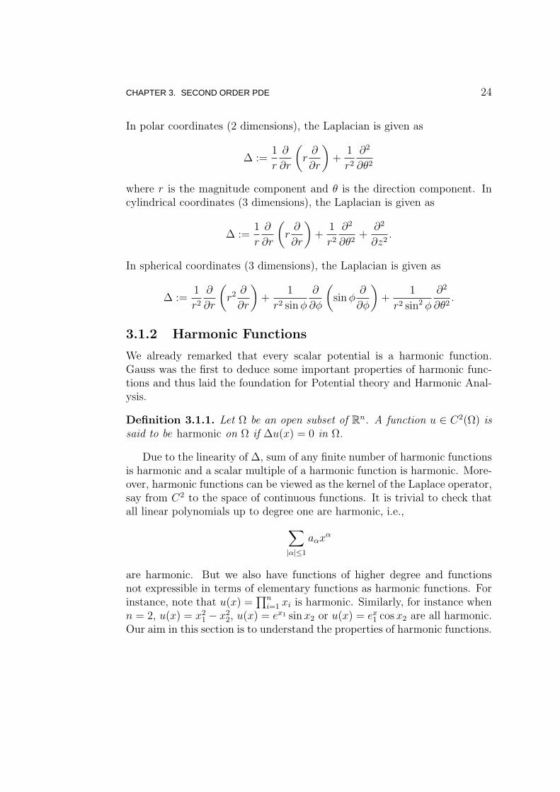
In polar coordinates (2 dimensions), the Laplacian is given as
∆ :=1
r
∂
∂r
(
r∂
∂r
)
+1
r2∂2
∂θ2
where r is the magnitude component and θ is the direction component. Incylindrical coordinates (3 dimensions), the Laplacian is given as
∆ :=1
r
∂
∂r
(
r∂
∂r
)
+1
r2∂2
∂θ2+
∂2
∂z2.
In spherical coordinates (3 dimensions), the Laplacian is given as
∆ :=1
r2∂
∂r
(
r2∂
∂r
)
+1
r2 sinφ
∂
∂φ
(
sinφ∂
∂φ
)
+1
r2 sin2 φ
∂2
∂θ2.
3.1.2 Harmonic Functions
We already remarked that every scalar potential is a harmonic function.Gauss was the first to deduce some important properties of harmonic func-tions and thus laid the foundation for Potential theory and Harmonic Anal-ysis.
Definition 3.1.1. Let Ω be an open subset of Rn. A function u ∈ C2(Ω) issaid to be harmonic on Ω if ∆u(x) = 0 in Ω.
Due to the linearity of ∆, sum of any finite number of harmonic functionsis harmonic and a scalar multiple of a harmonic function is harmonic. More-over, harmonic functions can be viewed as the kernel of the Laplace operator,say from C2 to the space of continuous functions. It is trivial to check thatall linear polynomials up to degree one are harmonic, i.e.,
∑
|α|≤1
aαxα
are harmonic. But we also have functions of higher degree and functionsnot expressible in terms of elementary functions as harmonic functions. Forinstance, note that u(x) =
∏ni=1 xi is harmonic. Similarly, for instance when
n = 2, u(x) = x21 − x22, u(x) = ex1 sin x2 or u(x) = ex1 cos x2 are all harmonic.Our aim in this section is to understand the properties of harmonic functions.

CHAPTER 3. SECOND ORDER PDE 25
In fact, we shall note later that any harmonic function is C∞. Also, notethat if u is a harmonic function on Ω then, by Gauss divergence theorem (cf.Theorem C.0.7,
∫
∂Ω
∂u
∂νdσ = 0.
Definition 3.1.2. Let Ω be an open subset of Rn and wn = 2πn/2
Γ(n/2)(cf. Ap-
pendix B) be the surface area of the unit sphere S1(0) of Rn.
(a) A function u ∈ C(Ω) is said to satisfy the first mean value property(I-MVP) in Ω if
u(x) =1
ωnrn−1
∫
Sr(x)
u(y) dσy for any Br(x) ⊂ Ω.
(b) A function u ∈ C(Ω) is said to satisfy the second mean value property(II-MVP) in Ω if
u(x) =n
ωnrn
∫
Br(x)
u(y) dy for any Br(x) ⊂ Ω.
Exercise 1. Show that u satisfies the I-MVP iff
u(x) =1
ωn
∫
S1(0)
u(x+ rz) dσz.
Similarly, u satisfies II-MVP iff
u(x) =n
ωn
∫
B1(0)
u(x+ rz) dz.
Exercise 2. Show that the first MVP and second MVP are equivalent. Thatis show that u satisfies (a) iff u satisfies (b).
Owing to the above exercise we shall, henceforth, refer to the I-MVP andII-MVP as just mean value property (MVP).
We shall now prove a result on the smoothness of a function satisfyingMVP.
Theorem 3.1.3. If u ∈ C(Ω) satisfies the MVP in Ω, then u ∈ C∞(Ω).

CHAPTER 3. SECOND ORDER PDE 26
Proof. We first consider uε := ρε ∗ u, the convolution of u with mollifiers, asintroduced in Theorem D.0.9. where
Ωε := x ∈ Ω | dist(x, ∂Ω) > ε.
We shall now show that u = uε for all ε > 0, due to the MVP of u and theradial nature of ρ. Let x ∈ Ωε. Consider
uε(x) =
∫
Ω
ρε(x− y)u(y) dy
=
∫
Bε(x)
ρε(x− y)u(y) dy (Since supp(ρε) is in Bε(x))
=
∫ ε
0
ρε(r)
(∫
Sr(x)
u(y) dσy
)
dr (cf. Theorem B.0.2)
= u(x)ωn
∫ ε
0
ρε(r)rn−1 dr (Using MVP of u)
= u(x)
∫ ε
0
ρε(r)
(∫
Sr(0)
dσy
)
dr
= u(x)
∫
Bε(0)
ρε(y) dy = u(x).
Thus uε(x) = u(x) for all x ∈ Ωε and for all ε > 0. Since uε ∈ C∞(Ωε) forall ε > 0 (cf. Theorem D.0.9), we have u ∈ C∞(Ωε) for all ε > 0.
Theorem 3.1.4. Let u be a harmonic function on Ω. Then u satisfies theMVP in Ω.
Proof. Let Br(x) ⊂ Ω be any ball with centre at x ∈ Ω and for some r > 0.For the given harmonic function u, we set
v(r) :=1
ωnrn−1
∫
Sr(x)
u(y) dσy.
Note that v is not defined at 0, since r > 0. We have from Exercise 1 that
v(r) =1
ωn
∫
S1(0)
u(x+ rz) dσz.

CHAPTER 3. SECOND ORDER PDE 27
Now, differentiating both sides w.r.t r, we get
dv(r)
dr=
1
ωn
∫
S1(0)
∇u(x+ rz) · z dσz
=1
ωnrn−1
∫
Sr(x)
∇u(y) · (y − x)
rdσy
Since |x− y| = r, by setting ν := (y − x)/r as the unit vector, and applyingthe Gauss divergence theorem along with the fact that u is harmonic, we get
dv(r)
dr=
1
ωnrn−1
∫
Sr(x)
∇u(y) · ν dσy =1
ωnrn−1
∫
Br(x)
∆u(y) dy = 0.
Thus, v is a constant function of r > 0 and hence
v(r) = v(ε) ∀ε > 0.
Moreover, since v is continuous (constant function), we have
v(r) = limε→0
v(ε)
= limε→0
1
ωn
∫
S1(0)
u(x+ εz) dσz
=1
ωn
∫
S1(0)
limε→0
u(x+ εz) dσz (u is continuous on S1(0))
=1
ωn
∫
S1(0)
u(x) dσz
= u(x) (Since ωn is the surface area of S1(0)).
Thus, u satisfies I-MVP and hence the II-MVP.
Corollary 3.1.5. If u is harmonic on Ω, then u ∈ C∞(Ω).
The above corollary is a easy consequence of Theorem 3.1.4 and Theo-rem 3.1.3. We shall now prove that any function satisfying MVP is harmonic.
Theorem 3.1.6. If u ∈ C(Ω) satisfies the MVP in Ω, then u is harmonicin Ω.
CHAPTER 3. SECOND ORDER PDE 28
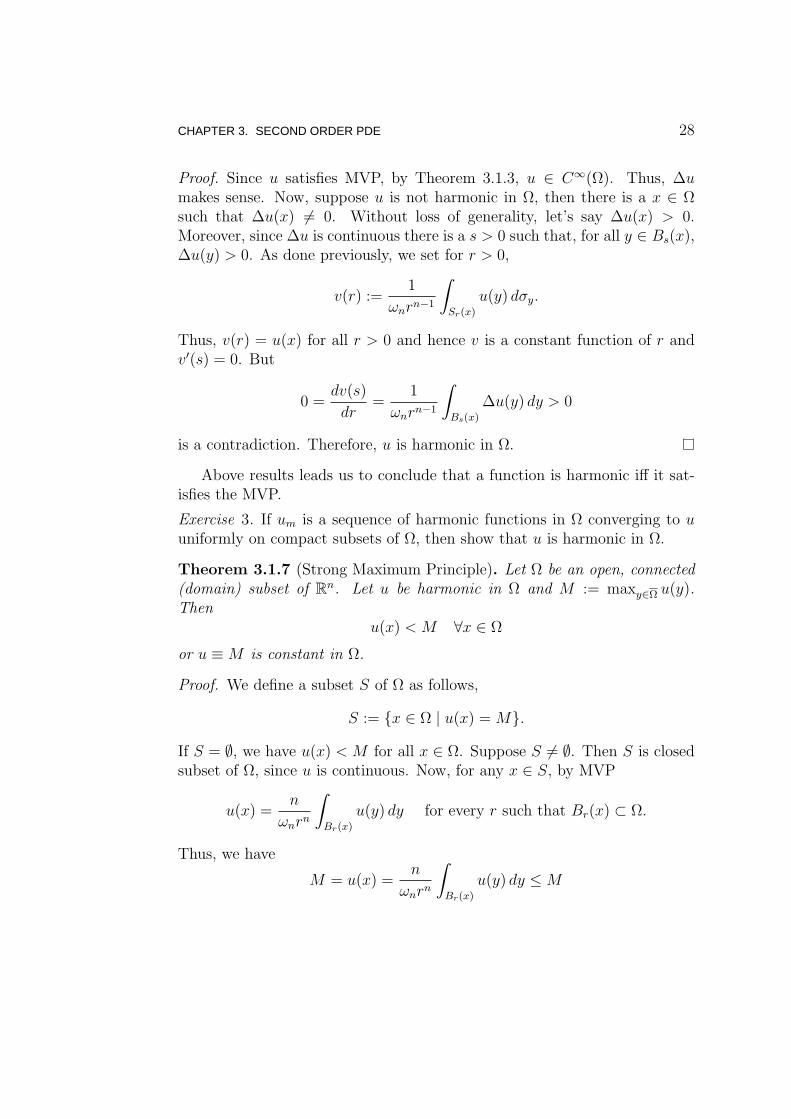
Proof. Since u satisfies MVP, by Theorem 3.1.3, u ∈ C∞(Ω). Thus, ∆umakes sense. Now, suppose u is not harmonic in Ω, then there is a x ∈ Ωsuch that ∆u(x) 6= 0. Without loss of generality, let’s say ∆u(x) > 0.Moreover, since ∆u is continuous there is a s > 0 such that, for all y ∈ Bs(x),∆u(y) > 0. As done previously, we set for r > 0,
v(r) :=1
ωnrn−1
∫
Sr(x)
u(y) dσy.
Thus, v(r) = u(x) for all r > 0 and hence v is a constant function of r andv′(s) = 0. But
0 =dv(s)
dr=
1
ωnrn−1
∫
Bs(x)
∆u(y) dy > 0
is a contradiction. Therefore, u is harmonic in Ω.
Above results leads us to conclude that a function is harmonic iff it sat-isfies the MVP.
Exercise 3. If um is a sequence of harmonic functions in Ω converging to uuniformly on compact subsets of Ω, then show that u is harmonic in Ω.
Theorem 3.1.7 (Strong Maximum Principle). Let Ω be an open, connected(domain) subset of R
n. Let u be harmonic in Ω and M := maxy∈Ω u(y).Then
u(x) < M ∀x ∈ Ω
or u ≡M is constant in Ω.
Proof. We define a subset S of Ω as follows,
S := x ∈ Ω | u(x) =M.
If S = ∅, we have u(x) < M for all x ∈ Ω. Suppose S 6= ∅. Then S is closedsubset of Ω, since u is continuous. Now, for any x ∈ S, by MVP
u(x) =n
ωnrn
∫
Br(x)
u(y) dy for every r such that Br(x) ⊂ Ω.
Thus, we have
M = u(x) =n
ωnrn
∫
Br(x)
u(y) dy ≤M

CHAPTER 3. SECOND ORDER PDE 29
Hence equality will hold above only when u(y) =M for all y ∈ Br(x). Thus,we have shown that for any x ∈ S, we have Br(x) ⊂ S. Therefore, S is open.Since Ω is connected, the only open and closed subsets are ∅ or Ω. SinceS was assumed to be non-empty, we should have S = Ω. Thus, u ≡ M isconstant in Ω.
Corollary 3.1.8 (Weak maximum Principle). Let Ω be an open, boundedsubset of Rn. Let u ∈ C(Ω) be harmonic in Ω. Then
maxy∈Ω
u(y) = maxy∈∂Ω
u(y).
Proof. Let M := maxy∈Ω u(y). If there is a x ∈ Ω such that u(x) =M , thenu ≡ M is constant on the connected component of Ω containing x. Thus,u = M on the boundary of the connected component which is a part of∂Ω.
Theorem 3.1.9 (Uniqueness of Harmonic Functions). Let Ω be an open,bounded subset of Rn. Let u1, u2 ∈ C(Ω) be harmonic in Ω such that u1 = u2on ∂Ω, then u1 = u2 in Ω.
Proof. Note that u1−u2 is a harmonic function and hence, by weak maximumprinciple, should attain its maximum on ∂Ω. But u1 − u2 = 0 on ∂Ω. Thusu1 − u2 ≤ 0 in Ω. Now, repeat the argument for u2 − u1, we get u2 − u1 ≤ 0in Ω. Thus, we get u1 − u2 = 0 in Ω.
Theorem 3.1.10 (Estimates on derivatives). If u is harmonic in Ω, then
|Dαu(x)| ≤ Ck
rn+k‖u‖1,Br(x) ∀Br(x) ⊂ Ω and each |α| = k
where the constants C0 =nωn
and Ck = C0(2n+1nk)k for k = 1, 2, . . ..
Proof. We prove the result by induction on k. Let k = 0. Since u is harmonic,by II-MVP we have, for any Br(x) ⊂ Ω,
|u(x)| =n
ωnrn
∣
∣
∣
∣
∫
Br(x)
u(y) dy
∣
∣
∣
∣
≤ n
ωnrn
∫
Br(x)
|u(y)| dy
=n
ωnrn‖u‖1,Br(x) =
C0
rn‖u‖1,Br(x).

CHAPTER 3. SECOND ORDER PDE 30
Now, let k = 1. Observe that if u is harmonic then by differentiating theLaplace equation and using the equality of mixed derivatives, we have uxi
:=∂u∂xi
is harmoic, for all i = 1, 2, . . . , n. Now, by the II-MVP of uxi, we have
|uxi(x)| =
n2n
ωnrn
∣
∣
∣
∣
∣
∫
Br/2(x)
uxi(y) dy
∣
∣
∣
∣
∣
=n2n
ωnrn
∣
∣
∣
∣
∣
∫
Sr/2(x)
uνi dσy
∣
∣
∣
∣
∣
(by Gauss-Green theorem)
≤ 2n
r‖u‖∞,Sr/2(x).
Thus, it now remains to estimate ‖u‖∞,Sr/2(x). Let z ∈ Sr/2(x), thenBr/2(z) ⊂Br(x) ⊂ Ω. But, using k = 0 result, we have
|u(z)| ≤ C02n
rn‖u‖1,Br/2(z) ≤
C02n
rn‖u‖1,Br(x).
Therefore, ‖u‖∞,Sr/2(x) ≤ C02n
rn‖u‖1,Br(x) and using this in the estimate of uxi
,we get
|uxi(x)| ≤ C0n2
n+1
rn+1‖u‖1,Br(x).
Hence
|Dαu(x)| ≤ C1
rn+1‖u‖1,Br(x) for |α| = 1.
Let now k ≥ 2 and α be a multi-index such that |α| = k. We assume theinduction hypothesis that the estimate to be proved is true for k − 1. Notethat Dαu = ∂Dβu
∂xifor some i ∈ 1, 2, . . . , n and |β| = k − 1. Moreover,
if u is harmonic then by differentiating the Laplace equation and using theequality of mixed derivatives, we have ∂Dβu
∂xiis harmoic for i = 1, 2, . . . , n.
Thus, following an earlier argument, we have
|Dαu(x)| =∣
∣
∣
∣
∂Dβu(x)
∂xi
∣
∣
∣
∣
=nkn
ωnrn
∣
∣
∣
∣
∣
∫
Br/k(x)
∂Dβu(y)
∂xidy
∣
∣
∣
∣
∣
=nkn
ωnrn
∣
∣
∣
∣
∣
∫
Sr/k(x)
Dβuνi dσy
∣
∣
∣
∣
∣
(by Gauss-Green theorem)
≤ nk
r‖Dβu‖∞,Sr/k(x).
CHAPTER 3. SECOND ORDER PDE 31
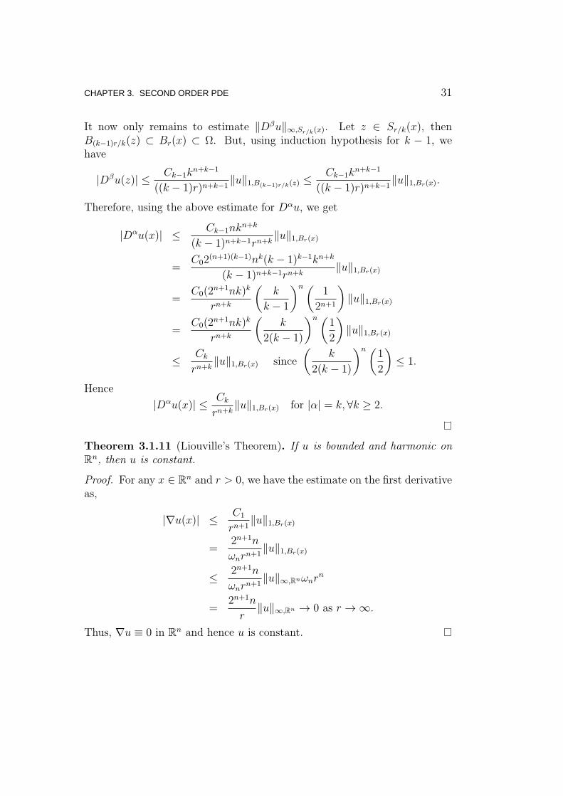
It now only remains to estimate ‖Dβu‖∞,Sr/k(x). Let z ∈ Sr/k(x), thenB(k−1)r/k(z) ⊂ Br(x) ⊂ Ω. But, using induction hypothesis for k − 1, wehave
|Dβu(z)| ≤ Ck−1kn+k−1
((k − 1)r)n+k−1‖u‖1,B(k−1)r/k(z) ≤
Ck−1kn+k−1
((k − 1)r)n+k−1‖u‖1,Br(x).
Therefore, using the above estimate for Dαu, we get
|Dαu(x)| ≤ Ck−1nkn+k
(k − 1)n+k−1rn+k‖u‖1,Br(x)
=C02
(n+1)(k−1)nk(k − 1)k−1kn+k
(k − 1)n+k−1rn+k‖u‖1,Br(x)
=C0(2
n+1nk)k
rn+k
(
k
k − 1
)n(1
2n+1
)
‖u‖1,Br(x)
=C0(2
n+1nk)k
rn+k
(
k
2(k − 1)
)n(1
2
)
‖u‖1,Br(x)
≤ Ck
rn+k‖u‖1,Br(x) since
(
k
2(k − 1)
)n(1
2
)
≤ 1.
Hence
|Dαu(x)| ≤ Ck
rn+k‖u‖1,Br(x) for |α| = k, ∀k ≥ 2.
Theorem 3.1.11 (Liouville’s Theorem). If u is bounded and harmonic onR
n, then u is constant.
Proof. For any x ∈ Rn and r > 0, we have the estimate on the first derivative
as,
|∇u(x)| ≤ C1
rn+1‖u‖1,Br(x)
=2n+1n
ωnrn+1‖u‖1,Br(x)
≤ 2n+1n
ωnrn+1‖u‖∞,Rnωnr
n
=2n+1n
r‖u‖∞,Rn → 0 as r → ∞.
Thus, ∇u ≡ 0 in Rn and hence u is constant.
CHAPTER 3. SECOND ORDER PDE 32
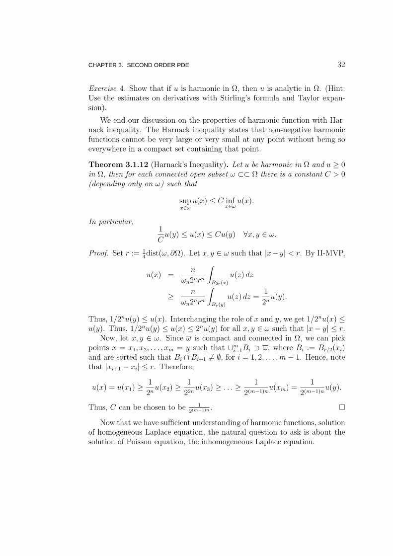
Exercise 4. Show that if u is harmonic in Ω, then u is analytic in Ω. (Hint:Use the estimates on derivatives with Stirling’s formula and Taylor expan-sion).
We end our discussion on the properties of harmonic function with Har-nack inequality. The Harnack inequality states that non-negative harmonicfunctions cannot be very large or very small at any point without being soeverywhere in a compact set containing that point.
Theorem 3.1.12 (Harnack’s Inequality). Let u be harmonic in Ω and u ≥ 0in Ω, then for each connected open subset ω ⊂⊂ Ω there is a constant C > 0(depending only on ω) such that
supx∈ω
u(x) ≤ C infx∈ω
u(x).
In particular,1
Cu(y) ≤ u(x) ≤ Cu(y) ∀x, y ∈ ω.
Proof. Set r := 14dist(ω, ∂Ω). Let x, y ∈ ω such that |x−y| < r. By II-MVP,
u(x) =n
ωn2nrn
∫
B2r(x)
u(z) dz
≥ n
ωn2nrn
∫
Br(y)
u(z) dz =1
2nu(y).
Thus, 1/2nu(y) ≤ u(x). Interchanging the role of x and y, we get 1/2nu(x) ≤u(y). Thus, 1/2nu(y) ≤ u(x) ≤ 2nu(y) for all x, y ∈ ω such that |x− y| ≤ r.
Now, let x, y ∈ ω. Since ω is compact and connected in Ω, we can pickpoints x = x1, x2, . . . , xm = y such that ∪m
i=1Bi ⊃ ω, where Bi := Br/2(xi)and are sorted such that Bi ∩ Bi+1 6= ∅, for i = 1, 2, . . . ,m− 1. Hence, notethat |xi+1 − xi| ≤ r. Therefore,
u(x) = u(x1) ≥1
2nu(x2) ≥
1
22nu(x3) ≥ . . . ≥ 1
2(m−1)nu(xm) =
1
2(m−1)nu(y).
Thus, C can be chosen to be 12(m−1)n .
Now that we have sufficient understanding of harmonic functions, solutionof homogeneous Laplace equation, the natural question to ask is about thesolution of Poisson equation, the inhomogeneous Laplace equation.

CHAPTER 3. SECOND ORDER PDE 33
3.2 Poisson Equation in Rn
We now wish to solve the Poisson equation, for any given f (under somehypothesis) find u such that
−∆u = f in Rn. (3.2.1)
Recall that we have already introduced the notion convolution of functions(cf. Appendix D) while discussing C∞ properties of harmonic functions. Wealso observed that the differential operator can be accumulated either side inthe convolution operation. Suppose there is a “function”K with the propertythat ∆K is the identity of the convolution operation, i.e., f ∗∆K = f , thenwe know that u := f ∗K is a solution of (3.2.1).
Definition 3.2.1. We shall say a “function” K to be the fundamental solu-tion of the Laplacian, ∆, if ∆K is the identity with respect to the convolutionoperation.
We caution that the above definition is not mathematically precise be-cause we made no mention on what the “function” K could be and its dif-ferentiability, even its existence is under question. We shall just take it as ainformal definition.
The question of interest is: can one find a K with above property? Toanswer this, let us observe that since we want K such that f ∗∆K for all fin the given space of functions in R
n. In particular, one can choose f ≡ 1.Thus, we are looking for K such that 1 ∗∆K = 1, i.e.,
∫
Rn
∆K = 1.
Equivalently, we want K such that
limr→∞
∫
Br(0)
∆K = 1,
which by Gauss divergence theorem (all informally) means we look for Ksuch that
limr→∞
∫
Sr(0)
∇K · ν = 1.

CHAPTER 3. SECOND ORDER PDE 34
3.2.1 Fundamental Solution of Laplacian
The Laplace operator is invariant under coordinate translation and rotation.Suppose x ∈ R
n is translated by a vector a ∈ Rn. Then the Laplace operator
is invariant of translation. That is, if ∆u(x) = f(x), then ∆u(x + a) =f(x+a). Similarly, for any rotation, the Laplace operator remains unchanged,i.e., if ∆u(r, θ) = f(r, θ), then ∆u(r, θ + η) = f(r, θ + η).
Exercise 5. If Ta is a translation of a vector by a, i.e., Ta(x) = x + a and if∆u(x) = f(x), then show that ∆u(Ta(x)) = f(Ta(x)). Also, if O is a n × northogonal matrix and if ∆u(x) = f(x), then show that ∆u(Ox) = f(Ox).
Thus, we say the Laplacian commutes with translation and rotation. Aradial function is constant on every sphere about the origin. Since Laplaciancommutes with rotations, it should map the class of all radial functions toitself. The invariance of Laplacian under rotation motivates us to look for aradial fundamental solution. To do so, we shall understand how Laplaciantreats radial functions.
Proposition 3.2.2. If u is a radial function, i.e., u(x) = u(r) where x ∈ Rn
and r = |x|, then
∆u(x) =d2u(r)
dr2+
(n− 1)
r
du(r)
dr.
Proof. Note that
∂r
∂xi=∂|x|∂xi
=∂(√
x21 + . . .+ x2n)
∂xi
=1
2(x21 + . . .+ x2n)
−1/2(2xi)
=xir.
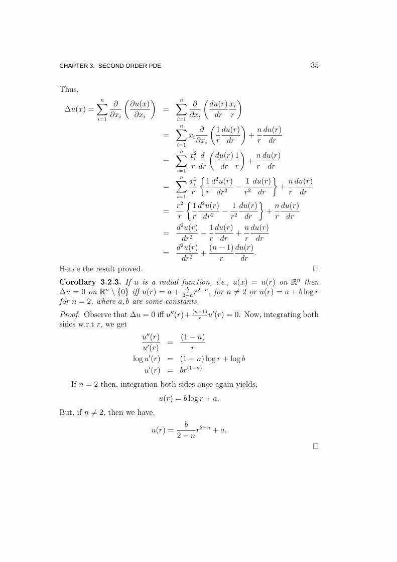
CHAPTER 3. SECOND ORDER PDE 35
Thus,
∆u(x) =n∑
i=1
∂
∂xi
(
∂u(x)
∂xi
)
=n∑
i=1
∂
∂xi
(
du(r)
dr
xir
)
=n∑
i=1
xi∂
∂xi
(
1
r
du(r)
dr
)
+n
r
du(r)
dr
=n∑
i=1
x2ir
d
dr
(
du(r)
dr
1
r
)
+n
r
du(r)
dr
=n∑
i=1
x2ir
1
r
d2u(r)
dr2− 1
r2du(r)
dr
+n
r
du(r)
dr
=r2
r
1
r
d2u(r)
dr2− 1
r2du(r)
dr
+n
r
du(r)
dr
=d2u(r)
dr2− 1
r
du(r)
dr+n
r
du(r)
dr
=d2u(r)
dr2+
(n− 1)
r
du(r)
dr.
Hence the result proved.
Corollary 3.2.3. If u is a radial function, i.e., u(x) = u(r) on Rn then
∆u = 0 on Rn \ 0 iff u(r) = a + b
2−nr2−n, for n 6= 2 or u(r) = a + b log r
for n = 2, where a, b are some constants.
Proof. Observe that ∆u = 0 iff u′′(r)+ (n−1)ru′(r) = 0. Now, integrating both
sides w.r.t r, we get
u′′(r)
u′(r)=
(1− n)
r
log u′(r) = (1− n) log r + log b
u′(r) = br(1−n)
If n = 2 then, integration both sides once again yields,
u(r) = b log r + a.
But, if n 6= 2, then we have,
u(r) =b
2− nr2−n + a.

CHAPTER 3. SECOND ORDER PDE 36
The reason to choose the domain of the Laplacian as Rn \ 0 is becausethe operator involves a ‘r’ in the denominator. However, for one dimensionalcase we can let zero to be on the domain of Laplacian, since for n = 1, theLaplace operator is unchanged. Thus, for n = 1, u(x) = a+ bx is a harmonicfunction in R
n.Note that as r → 0, u(r) → ∞. Thus, u has a singularity at 0. In fact,
for any given w ∈ Rn, ∆u(x−w) = 0 for all x ∈ R
n \ w. By special choiceof constants a, b, we shall define the radial fundamental solution. We shallchoose a, b such that for every sphere Sr(0) about the origin, we have
∫
Sr(0)
d
dru(r) dσ = 1.
Thus,
1 =
∫
Sr(0)
d
dru(r) dσ =
b
2− n
d
drr2−n
∫
Sr(0)
dσ
= br1−nrn−1ωn.
Thus, we choose b = 1ωn
and a ≡ 0, for n 6= 2 and for n = 2, we choose
a ≡ 0 and b = 12π. For convention sake, we shall add minus (“−”) sign (notice
the minus sign in (3.2.1)).
Definition 3.2.4. We say K(x), defined as
K(x) :=
− 12π
log |x| (n = 2)|x|2−n
ωn(n−2)(n ≥ 3),
is the fundamental solution of the Laplacian.
We end this section by emphasising that the notion of fundamental so-lution has a precise definition in terms of the Dirac measure. The Diracmeasure, at a point x ∈ R
n, is defined as,
δx(E) =
1 if x ∈ E
0 if x /∈ E
for all measurable subsets E of the measure space Rn. The Dirac measure
has the property that∫
E
dδx = 1

CHAPTER 3. SECOND ORDER PDE 37
if x ∈ E and zero if x /∈ E. Also, for any integrable function f ,
∫
Rn
f(y) dδx = f(x).
In this new set-up a fundamental solution K can be defined as the solutioncorresponding to δx, i.e.,
−∆K = δx in Rn.
Note that the above equation, as such, makes no sense because the RHS is aset-function taking subsets of Rn as arguments, whereas K is a function onR
n. To give meaning to above equation, one needs to view δx as a distribution(introduced by L. Schwartz) and the equation should be interpreted in thedistributional derivative sense. The Dirac measure is the distributional limitof the sequence of mollifiers, ρε, in the space of distributions.
3.2.2 Solving Poisson Equation
In this section, we shall give a formula for the solution of the Poisson equation(3.2.1) in R
n in terms of the fundamental solution.
Theorem 3.2.5. For any given f ∈ C2c (R
n), u := K ∗ f is a solution to thePoisson equation (3.2.1).
Proof. By the property of convolution (cf. proof of Theorem D.0.9), we knowthat Dαu(x) = (K ∗ Dαf)(x) for all |α| ≤ 2. Since f ∈ C2
c (Rn), we have
u ∈ C2(Rn. The difficulty arises due to the singularity of K at the origin.

CHAPTER 3. SECOND ORDER PDE 38
Consider, for any fixed m > 0,
∆u(x) =
∫
Rn
K(y)∆xf(x− y) dy
=
∫
Bm(0)
K(y)∆xf(x− y) dy +
∫
Rn\Bm(0)
K(y)∆xf(x− y) dy
=
∫
Bm(0)
K(y)∆xf(x− y) dy +
∫
Rn\Bm(0)
K(y)∆yf(x− y) dy
=
∫
Bm(0)
K(y)∆xf(x− y) dy +
∫
Sm(0)
K(y)∇yf(x− y) · ν dσy
−∫
Rn\Bm(0)
∇yK(y) · ∇yf(x− y) dy (cf. Corollary C.0.8)
=
∫
Bm(0)
K(y)∆xf(x− y) dy +
∫
Sm(0)
K(y)∇yf(x− y) · ν dσy
+
∫
Rn\Bm(0)
∆yK(y)f(x− y) dy −∫
Sm(0)
f(x− y)∇yK(y) · ν dσy
(cf. Corollary C.0.8)
=
∫
Bm(0)
K(y)∆xf(x− y) dy +
∫
Sm(0)
K(y)∇yf(x− y) · ν dσy
−∫
Sm(0)
f(x− y)∇yK(y) · ν dσy
:= Im(x) + Jm(x) +Km(x).
But, due to the compact support of f , we have
|Im(x)| ≤ ‖D2f‖∞,Rn
∫
Bm(0)
|K(y)| dy.
Thus, for n = 2,
|Im(x)| ≤m2
2
(
1
2+ | logm|
)
‖D2f‖∞,Rn
and for n ≥ 3, we have
|Im(x)| ≤m2
2(n− 2)‖D2f‖∞,Rn .

CHAPTER 3. SECOND ORDER PDE 39
Hence, as m→ 0, |Im(x)| → 0. Similarly,
|Jm(x)| ≤∫
Sm(0)
|K(y)∇yf(x− y) · ν| dσy
≤ ‖∇f‖∞,Rn
∫
Sm(0)
|K(y)| dσy.
Thus, for n = 2,|Jm(x)| ≤ m| logm|‖∇f‖∞,Rn
and for n ≥ 3, we have
|Jm(x)| ≤m
(n− 2)‖∇f‖∞,Rn .
Hence, as m→ 0, |Jm(x)| → 0. Now, to tackle the last term Km(x), we notethat a simple computation yields that ∇yK(y) = −1
ωn|y|ny. Since we are in
the m radius sphere |y| = m. Also the unit vector ν outside of Sm(0), as aboundary of Rn \Bm(0), is given by −y/|y| = −y/m. Therefore,
∇yK(y) · ν =1
ωnmn+1y · y =
1
ωnmn−1.
Km(x) = −∫
Sm(0)
f(x− y)∇yK(y) · ν dσy
=−1
ωnmn−1
∫
Sm(0)
f(x− y) dσy
=−1
ωnmn−1
∫
Sm(x)
f(y) dσy
Since f is continuous, for every ε > 0, there is a δ > 0 such that |f(x) −f(y)| < ε whenever |x − y| < δ. When m → 0, we can choose m such thatm < δ and for this m, we see that Now, consider
|Km(x)− (−f(x))| =
∣
∣
∣
∣
f(x)− 1
ωnmn−1
∫
Sm(x)
f(y) dσy
∣
∣
∣
∣
=1
ωnmn−1
∫
Sm(x)
|f(x)− f(y)| dσy < ε.
Thus, as m→ 0, Km(x) → −f(x). Hence, u solves (3.2.1).

CHAPTER 3. SECOND ORDER PDE 40
Remark 3.2.6. Notice that in the proof above, we have used the Green’sidentity eventhough our domain is not bounded (which is a hypothesis forGreen’s identity). This can be justified by taking a ball bigger that Bm(0)and working in the annular region, and later letting the bigger ball approachall of Rn.
A natural question at this juncture is: Is every solution of the Poissonequation (3.2.1) of the form K ∗ f . We answer this question in the followingtheorem.
Theorem 3.2.7. Let f ∈ C2c (R
n) and n ≥ 3. If u is a solution of (3.2.1)and u is bounded, then u has the form u(x) = (K ∗f)(x)+C, for any x ∈ R
n,where C is some constant.
Proof. We know that (cf. Theorem 3.2.5) u′(x) := (K ∗ f)(x) solves (3.2.1),the Poisson equation in R
n. Moreover, u′ is bounded for n ≥ 3, since K(x) →0 as |x| → ∞ and f has compact support in R
n. Also, since u is given to bea bounded solution of (3.2.1), v := u − u′ is a bounded harmonic function.Hence, by Liouville’s theorem, v is constant. Therefore u = u′ +C, for someconstant C.
3.3 Dirichlet Problem
We turn our attention to studying Poisson equation in proper subsets of Rn.Let Ω be an open bounded subset of Rn with C1 boundary ∂Ω.
The Dirichlet problem is stated as follows: Given f : Ω → R and g :∂Ω → R, find u : Ω → R such that
−∆u = f in Ωu = g on ∂Ω
(3.3.1)
Thus, we call the boundary condition imposed above to be the Dirichletboundary condition. Note that, by Theorem 3.1.9, the solution of Dirichletproblem, if it exists, is unique.
To begin with we shall focus on the study of Dirichlet problem. TheDirichlet problem can be solved in four different approaches, viz., usingGreen’s function, Dirichlet principle, layer potentials and L2-estimates. Thelast two approaches also solve Neumann problem.

CHAPTER 3. SECOND ORDER PDE 41
3.3.1 Green’s Function
To begin we shall motivate the derivation of Green’s function. For any x ∈ Ω,choose m > 0 such that Bm(x) ⊂ Ω. Set Ωm := Ω\Bm(x). Now applying thesecond identity of Corollary C.0.8 for any u ∈ C2(Ω) and v(y) = K(y − x),the fundamental solution on R
n \ x, on the domain Ωm, we get
∫
∂Ωm
(
u(y)∂K
∂ν(y − x)−K(y − x)
∂u(y)
∂ν
)
dσy =
∫
Ωm
u(y)∆yK(y − x) dy
−∫
Ωm
K(y − x)∆yu(y) dy
∫
∂Ωm
(
u(y)∂K
∂ν(y − x)−K(y − x)
∂u(y)
∂ν
)
dσy = −∫
Ωm
K(y − x)∆yu(y) dy
∫
∂Ω
(
u(y)∂K
∂ν(y − x)−K(y − x)
∂u(y)
∂ν
)
dσy
+
∫
Ω
K(y − x)∆yu(y) dy = −∫
Sm(x)
u(y)∂K
∂ν(y − x) dσy
+
∫
Sm(x)
K(y − x)∂u(y)
∂νdσy
+
∫
Bm(x)
K(y − x)∆yu(y) dy
= Km(x) + Jm(x) + Im(x)
The RHS is handled exactly as in the proof of Theorem 3.2.5, since u isa continuous function on the compact set Ω and is bounded. We repeat thearguments below for completeness sake.
Consider the first term Km(x). Note that ∇yK(y − x) = −1ωn|y−x|n
(y − x).
Since we are in the m radius sphere |y − x| = m. Also the unit vector νinside of Sm(x), as a boundary of Ω \Bm(x), is given by −(y − x)/|y − x| =−(y − x)/m. Therefore,
∇yK(y − x) · ν =1
ωnmn+1(y − x) · (y − x) =
1
ωnmn−1.

CHAPTER 3. SECOND ORDER PDE 42
Thus,
Km(x) = −∫
Sm(x)
u(y)∇yK(y − x) · ν dσy
=−1
ωnmn−1
∫
Sm(x)
u(y) dσy
Since u is continuous, for every ε > 0, there is a δ > 0 such that |u(x)−u(y)| <ε whenever |x − y| < δ. When m → 0, we can choose m such that m < δand for this m, we see that Now, consider
|Km(x)− (−u(x))| =
∣
∣
∣
∣
u(x)− 1
ωnmn−1
∫
Sm(x)
u(y) dσy
∣
∣
∣
∣
=1
ωnmn−1
∫
Sm(x)
|u(x)− u(y)| dσy < ε.
Thus, as m→ 0, Km(x) → −u(x).We next consider the term Jm(x),
|Jm(x)| ≤∫
Sm(x)
|K(y − x)∇yu(y) · ν| dσy
≤ ‖∇yu‖∞,Ω
∫
Sm(x)
|K(y − x)| dσy.
Thus, for n = 2,|Jm(x)| ≤ m| logm|‖∇yu‖∞,Ω
and for n ≥ 3, we have
|Jm(x)| ≤m
(n− 2)‖∇yu‖∞,Ω.
Hence, as m→ 0, |Jm(x)| → 0. We now consider the term Im.
|Im(x)| ≤ ‖D2u‖∞,Ω
∫
Bm(x)
|K(y − x)| dy.
Thus, for n = 2,
|Im(x)| ≤m2
2
(
1
2+ | logm|
)
‖D2u‖∞,Ω
CHAPTER 3. SECOND ORDER PDE 43
and for n ≥ 3, we have
|Im(x)| ≤m2
2(n− 2)‖D2u‖∞,Ω.
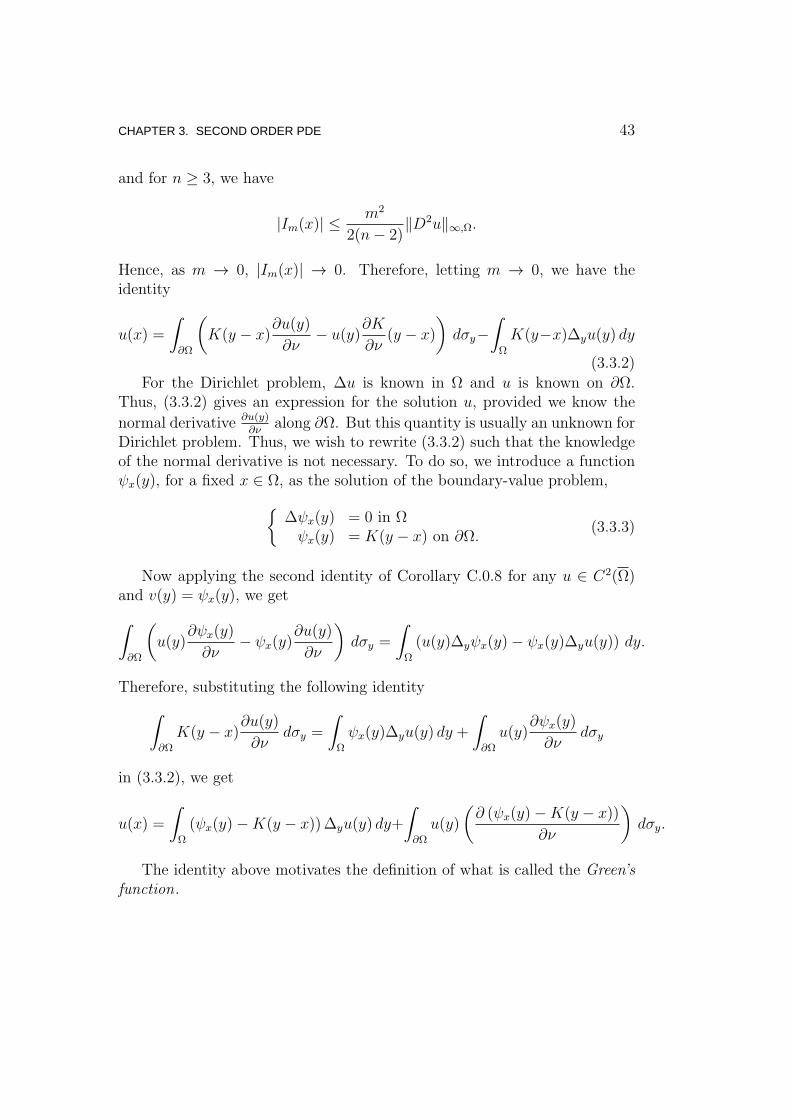
Hence, as m → 0, |Im(x)| → 0. Therefore, letting m → 0, we have theidentity
u(x) =
∫
∂Ω
(
K(y − x)∂u(y)
∂ν− u(y)
∂K
∂ν(y − x)
)
dσy−∫
Ω
K(y−x)∆yu(y) dy
(3.3.2)For the Dirichlet problem, ∆u is known in Ω and u is known on ∂Ω.
Thus, (3.3.2) gives an expression for the solution u, provided we know the
normal derivative ∂u(y)∂ν
along ∂Ω. But this quantity is usually an unknown forDirichlet problem. Thus, we wish to rewrite (3.3.2) such that the knowledgeof the normal derivative is not necessary. To do so, we introduce a functionψx(y), for a fixed x ∈ Ω, as the solution of the boundary-value problem,
∆ψx(y) = 0 in Ωψx(y) = K(y − x) on ∂Ω.
(3.3.3)
Now applying the second identity of Corollary C.0.8 for any u ∈ C2(Ω)and v(y) = ψx(y), we get
∫
∂Ω
(
u(y)∂ψx(y)
∂ν− ψx(y)
∂u(y)
∂ν
)
dσy =
∫
Ω
(u(y)∆yψx(y)− ψx(y)∆yu(y)) dy.
Therefore, substituting the following identity
∫
∂Ω
K(y − x)∂u(y)
∂νdσy =
∫
Ω
ψx(y)∆yu(y) dy +
∫
∂Ω
u(y)∂ψx(y)
∂νdσy
in (3.3.2), we get
u(x) =
∫
Ω
(ψx(y)−K(y − x))∆yu(y) dy+
∫
∂Ω
u(y)
(
∂ (ψx(y)−K(y − x))
∂ν
)
dσy.
The identity above motivates the definition of what is called the Green’sfunction.

CHAPTER 3. SECOND ORDER PDE 44
Definition 3.3.1. For any given open subset Ω ⊂ Rn and x, y ∈ Ω such that
x 6= y, we define the Green’s function as
G(x, y) := ψx(y)−K(y − x).
Rewriting (3.3.2) in terms of Green’s function,we get
u(x) =
∫
Ω
G(x, y)∆yu(y) dy +
∫
∂Ω
u(y)∂G(x, y)
∂νdσy.
Thus, in the arguments above we have proved the following theorem.
Theorem 3.3.2. Let Ω be a bounded open subset of Rn with C1 boundary.Also, given f ∈ C(Ω) and g ∈ C(Ω). If u ∈ C2(Ω) solves the Dirichletproblem (3.3.1), then u has the representation
u(x) = −∫
Ω
G(x, y)f(y) dy +
∫
∂Ω
g(y)∂G(x, y)
∂νdσy. (3.3.4)
Observe that we have solved the Dirichlet problem (3.3.1) provided weknow the Green’s function. The construction of Green’s function dependson the construction of ψx for every x ∈ Ω. In other words, (3.3.1) is solvedif we can solve (3.3.3). Ironically, computing ψx is usually possible when Ωhas simple geometry. We shall identify two simple cases of Ω, half-space andballl, where we can explicitly compute G.
The Green’s function is the analogue of the fundamental solution K forthe boundary value problem. This is clear by observing that, for a fixedx ∈ Ω, G satisfies (informally) the equation,
−∆G(x, ·) = δx in ΩG(x, ·) = 0 on ∂Ω,
where δx is the Dirac measure at x.
Theorem 3.3.3. For all x, y ∈ Ω such that x 6= y, we have G(x, y) = G(y, x),i.e., G is symmetric in x and y.
Proof. Let us fix x, y ∈ Ω. For a fixed m > 0, set Ωm = Ω \ (Bm(x)∪Bm(y))

CHAPTER 3. SECOND ORDER PDE 45
and applying Green’s identity for v(·) := G(x, ·) and w(·) := G(y, ·), we get
∫
∂Ωm
(
v(z)∂w(z)
∂ν− w(z)
∂v(z)
∂ν
)
dσz =
∫
Ωm
v(z)∆zw(z) dz
−∫
Ωm
w(z)∆zv(z) dz
∫
∂Ωm
(
v(z)∂w(z)
∂ν− w(z)
∂v(z)
∂ν
)
dσz = 0
∫
Sm(x)
(
v(z)∂w(z)
∂ν− w(z)
∂v(z)
∂ν
)
dσz =
∫
Sm(y)
(
w(z)∂v(z)
∂ν− v(z)
∂w(z)
∂ν
)
dσz
Jm(x) +Km(x) = Jm(y) +Km(y).
|Jm(x)| ≤∫
Sm(x)
|v(z)∇zw(z) · ν| dσz
≤ ‖∇w‖∞,Ω
∫
Sm(x)
|v(z)| dσz
= ‖∇w‖∞,Ω
∫
Sm(x)
|ψx(z)−K(z − x)| dσz.
Thus, for n = 2,
|Jm(x)| ≤ (2πm‖ψx‖∞,Ω +m| logm|) ‖∇w‖∞,Ω
and for n ≥ 3, we have
|Jm(x)| ≤(
ωnmn−1‖ψx‖∞,Ω +
m
(n− 2)
)
‖∇w‖∞,Ω.
Hence, as m→ 0, |Jm(x)| → 0. Now, consider the term Km(x),
Km(x) = −∫
Sm(x)
w(z)∂v(z)
∂νdσz
=
∫
Sm(x)
w(z)∂K
∂ν(z − x) dσz −
∫
Sm(x)
w(z)∂ψx(z)
∂νdσz.
The second term goes to zero by taking the sup-norm outside the integral.To tackle the first term, we note that ∇zK(z − x) = −1
ωn|z−x|n(z − x). Since

CHAPTER 3. SECOND ORDER PDE 46
we are in the m radius sphere |z − x| = m. Also the unit vector ν outside ofSm(x), as a boundary of Ω\Bm(x), is given by −(z−x)/|z−x| = −(z−x)/m.Therefore,
∇zK(z − x) · ν =1
ωnmn+1(z − x) · (z − x) =
1
ωnmn−1.
∫
Sm(x)
w(z)∇zK(z − x) · ν dσz =1
ωnmn−1
∫
Sm(x)
w(z) dσz
Since w is continuous in Ω \ y, for every ε > 0, there is a δ > 0 such that|w(z) − w(x)| < ε whenever |x − z| < δ. When m → 0, we can choose msuch that m < δ and for this m, we see that Now, consider
∣
∣
∣
∣
1
ωnmn−1
∫
Sm(x)
w(z) dσz − w(x)
∣
∣
∣
∣
=1
ωnmn−1
∫
Sm(x)
|w(z)− w(x)| dσz < ε.
Thus, as m → 0, Km(x) → w(x). Arguing similarly, for Jm(y) and Km(y),we get G(y, x) = G(x, y).
3.3.2 Green’s Function for half-space
In this section, we shall compute explicitly the Green’s function for positivehalf-space. Thus, we shall have
Rn+ = x = (x1, x2, . . . , xn) ∈ R
n | xn > 0
and∂Rn
+ = x = (x1, x2, . . . , xn ∈ Rn | xn = 0.
To compute the Green’s function, we shall use the method of reflection.The reflection technique ensures that the points on the boundary (alongwhich the reflection is done) remains unchanged to respect the imposedDirichlet condition.
Definition 3.3.4. For any x = (x1, x2, . . . , xn) ∈ Rn+, we define its reflection
along its boundary Rn−1 as x⋆ = (x1, x2, . . . ,−xn).

CHAPTER 3. SECOND ORDER PDE 47
It is obvious from the above definition that, for any y ∈ ∂Rn+, |y − x⋆| =
|y − x|. Given a fixed x ∈ Rn+, we need to find a harmonic function ψx in
Rn+, as in (3.3.3). But K(· − x) is harmonic in R
n+ \ x. Thus, we use the
method of reflection to shift the singularity of K from Rn+ to the negative
half-space and defineψx(y) = K(y − x⋆).
By definition, ψx is harmonic in Rn+ and on the boundary ψx(y) = K(y− x).
Therefore, we define the Green’s function to be G(x, y) = K(y−x⋆)−K(y−x), for all x, y ∈ R
n+ and x 6= y. It now only remains to compute the normal
derivative of G. Recall that ∇yK(y − x) = −1ωn|y−x|n
(y − x). Thus,
∇yG(x, y) =−1
ωn
(
y − x⋆
|y − x⋆|n − y − x
|y − x|n)
Therefore, when y ∈ ∂Rn+, we have
∇yG(x, y) =−1
ωn|y − x|n (x− x⋆).
Since the outward unit normal of ∂Rn+ is ν = (0, 0, . . . , 0,−1), we get
∇yG(x, y) · ν =2xn
ωn|y − x|n .
Definition 3.3.5. For all x ∈ Rn+ and y ∈ ∂Rn
+, the map
P (x, y) :=2xn
ωn|y − x|n
is called the Poisson kernel for Rn+.
Now substituing for G in (3.3.4), we get the Poisson formula for u,
u(x) =
∫
Rn+
[K(y − x)−K(y − x⋆)]f(y) dy +2xnωn
∫
∂Rn+
g(y)
|y − x|n dσy. (3.3.5)
It now remains to show that the u as defined above is, indeed, a solution of(3.3.1) for Rn
+.
Exercise 6. Let f ∈ C(Rn+) be given. Let g ∈ C(Rn−1) be bounded. Then u
as given in (3.3.5) is in C2(Rn+) and solves (3.3.1).

CHAPTER 3. SECOND ORDER PDE 48
3.3.3 Green’s Function for a disk
In this section, we shall compute explicitly the Green’s function for a ball ofradius r > 0 and centred at a ∈ R
n, Br(a). As usual, we denote the surfaceof the disk as Sr(a), the circle of radius r centred at a. We, once again, usethe method of reflection but, this time reflected along the boundary of thedisk.
Definition 3.3.6. For any x ∈ Rn \ a, we define its reflection along the
circle Sr(a) as x⋆ = r2(x−a)
|x−a|2+ a.
The idea behind reflection is clear for the unit disk, i.e., when a = 0 andr = 1, as x⋆ = x
|x|2. The above definition is just the shift of origin to a and
dilating the unit disk by r.Now, for any y ∈ Sr(a) and x 6= a, consider
|y − x⋆|2 = |y − a|2 − 2(y − a) · (x⋆ − a) + |x⋆ − a|2
= r2 − 2r2(y − a) ·(
x− a
|x− a|2)
+
∣
∣
∣
∣
r2(x− a)
|x− a|2∣
∣
∣
∣
2
=r2
|x− a|2 (|x− a|2 − 2(y − a) · (x− a) + r2)
=r2
|x− a|2 (|x− a|2 − 2(y − a) · (x− a) + |y − a|2)
=r2
|x− a|2 |y − x|2
Therefore, |x−a|r
|y−x⋆| = |y−x| for all y ∈ Sr(a). For each fixed x ∈ Br(a), weneed to find a harmonic function ψx in Br(a) solving (3.3.3). Since K(· − x)is harmonic in Br(a) \ x, we use the method of reflection to shift thesingularity of K at x to the complement of Br(a). Thus, we define
ψx(y) = K
( |x− a|r
(y − x⋆)
)
x 6= a.
For n ≥ 3, K(
|x−a|r
(y − x⋆))
= |x−a|2−n
r2−n K(y−x⋆). Thus, for n ≥ 3, ψx solves
(3.3.3), for x 6= a. For n = 2,
K
( |x− a|r
(y − x⋆)
)
=−1
2πlog
( |x− a|r
)
+K(y − x⋆).
CHAPTER 3. SECOND ORDER PDE 49
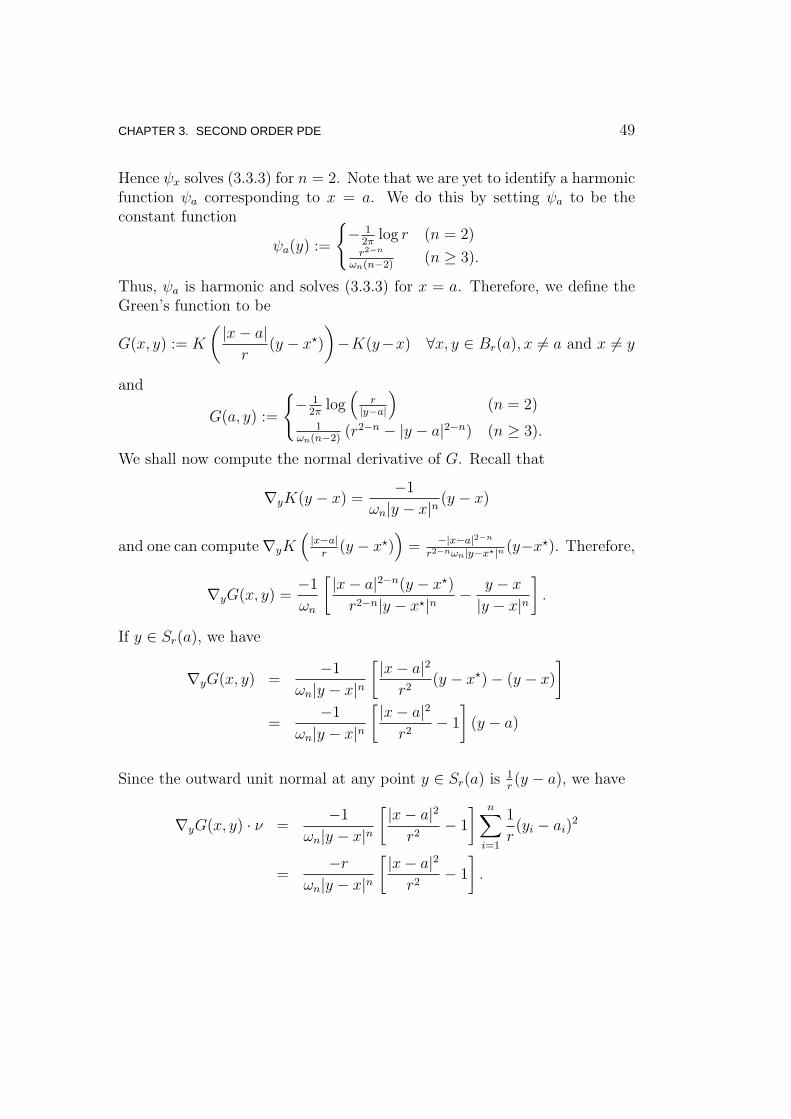
Hence ψx solves (3.3.3) for n = 2. Note that we are yet to identify a harmonicfunction ψa corresponding to x = a. We do this by setting ψa to be theconstant function
ψa(y) :=
− 12π
log r (n = 2)r2−n
ωn(n−2)(n ≥ 3).
Thus, ψa is harmonic and solves (3.3.3) for x = a. Therefore, we define theGreen’s function to be
G(x, y) := K
( |x− a|r
(y − x⋆)
)
−K(y−x) ∀x, y ∈ Br(a), x 6= a and x 6= y
and
G(a, y) :=
− 12π
log(
r|y−a|
)
(n = 2)
1ωn(n−2)
(r2−n − |y − a|2−n) (n ≥ 3).
We shall now compute the normal derivative of G. Recall that
∇yK(y − x) =−1
ωn|y − x|n (y − x)
and one can compute∇yK(
|x−a|r
(y − x⋆))
= −|x−a|2−n
r2−nωn|y−x⋆|n(y−x⋆). Therefore,
∇yG(x, y) =−1
ωn
[ |x− a|2−n(y − x⋆)
r2−n|y − x⋆|n − y − x
|y − x|n]
.
If y ∈ Sr(a), we have
∇yG(x, y) =−1
ωn|y − x|n[ |x− a|2
r2(y − x⋆)− (y − x)
]
=−1
ωn|y − x|n[ |x− a|2
r2− 1
]
(y − a)
Since the outward unit normal at any point y ∈ Sr(a) is1r(y − a), we have
∇yG(x, y) · ν =−1
ωn|y − x|n[ |x− a|2
r2− 1
] n∑
i=1
1
r(yi − ai)
2
=−r
ωn|y − x|n[ |x− a|2
r2− 1
]
.

CHAPTER 3. SECOND ORDER PDE 50
Definition 3.3.7. For all x ∈ Br(a) and y ∈ Sr(a), the map
P (x, y) :=r2 − |x− a|2rωn|y − x|n
is called the Poisson kernel for Br(a).
Now substituing for G in (3.3.4), we get the Poisson formula for u,
u(x) = −∫
Br(a)
G(x, y)f(y) dy +r2 − |x− a|2
rωn
∫
Sr(a)
g(y)
|y − x|n dσy. (3.3.6)
It now remains to show that the u as defined above is, indeed, a solution of(3.3.1) for Br(a).
Exercise 7. Let f ∈ C(Br(a)) be given. Let g ∈ C(Sr(a)) be bounded. Thenu as given in (3.3.6) is in C2(Br(a)) and solves (3.3.1).
3.3.4 Dirichlet principle
The Dirichlet principle (formulated, independently by Gauss, Lord Kelvinand Dirichlet) states that the solution of the Dirichlet problem minimizesthe corresponding energy functional.
Let Ω be an open bounded subset of Rn with C1 boundary ∂Ω and letf : Ω → R and g : ∂Ω → R be given. For convenience, recall the Dirichletproblem ((3.3.1)),
−∆u = f in Ωu = g on ∂Ω.
Any solution u of (3.3.1) is in V = v ∈ C2(Ω) | v = g on ∂Ω. Theenergy functional J : V → R is defined as
J(v) :=1
2
∫
Ω
|∇v|2 dx−∫
Ω
fv dx
Theorem 3.3.8 (Dirichlet’s principle). A C2(Ω) function u solves (3.3.1)iff u minimises the functional J on V , i.e.,
J(u) ≤ J(v) ∀v ∈ V.
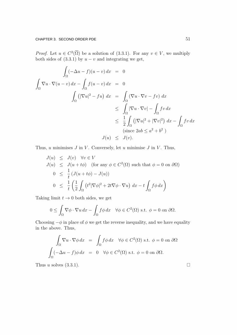
CHAPTER 3. SECOND ORDER PDE 51
Proof. Let u ∈ C2(Ω) be a solution of (3.3.1). For any v ∈ V , we multiplyboth sides of (3.3.1) by u− v and integrating we get,
∫
Ω
(−∆u− f)(u− v) dx = 0∫
Ω
∇u · ∇(u− v) dx−∫
Ω
f(u− v) dx = 0∫
Ω
(
|∇u|2 − fu)
dx =
∫
Ω
(∇u · ∇v − fv) dx
≤∫
Ω
|∇u · ∇v| −∫
Ω
fv dx
≤ 1
2
∫
Ω
(
|∇u|2 + |∇v|2)
dx−∫
Ω
fv dx
(since 2ab ≤ a2 + b2 )
J(u) ≤ J(v).
Thus, u minimises J in V . Conversely, let u minimise J in V . Thus,
J(u) ≤ J(v) ∀v ∈ V
J(u) ≤ J(u+ tφ) (for any φ ∈ C2(Ω) such that φ = 0 on ∂Ω)
0 ≤ 1
t(J(u+ tφ)− J(u))
0 ≤ 1
t
(
1
2
∫
Ω
(
t2|∇φ|2 + 2t∇φ · ∇u)
dx− t
∫
Ω
fφ dx
)
Taking limit t→ 0 both sides, we get
0 ≤∫
Ω
∇φ · ∇u dx−∫
Ω
fφ dx ∀φ ∈ C2(Ω) s.t. φ = 0 on ∂Ω.
Choosing −φ in place of φ we get the reverse inequality, and we have equalityin the above. Thus,
∫
Ω
∇u · ∇φ dx =
∫
Ω
fφ dx ∀φ ∈ C2(Ω) s.t. φ = 0 on ∂Ω∫
Ω
(−∆u− f)φ dx = 0 ∀φ ∈ C2(Ω) s.t. φ = 0 on ∂Ω.
Thus u solves (3.3.1).

CHAPTER 3. SECOND ORDER PDE 52
3.4 Neumann Problem
The Neumann problem is stated as follows: Given f : Ω → R and g : ∂Ω →R, find u : Ω → R such that
−∆u = f in Ω∂u∂ν
= g on ∂Ω(3.4.1)
where ∂u∂ν
:= ∇u · ν and ν = (ν1, . . . , νn) is the outward pointing unit normalvector field of ∂Ω. Thus, the boundary imposed is called the Neumannboundary condition. The solution of a Neumann problem is not necessarilyunique. If u is any solution of (3.4.1), then u+ c for any constant c is also asolution of (3.4.1). More generally, for any v such that v is constant on theconnected components of Ω, u+ v is a solution of (3.4.1). Moreover, if u is asolution of the Neumann problem (3.4.1) then u satisfies, for every connectedcomponent ω of Ω,
∫
ω
∆u =
∫
∂ω
∇u · ν (Using GDT)∫
ω
f =
∫
∂ω
g.
The second equality is called the compatibility condition. Thus, if (3.4.1) issolvable then necessarily, the given function f, g must satisfy the compatibil-ity condition.
3.5 Heat Equation
Let a homogeneous material occupy a region Ω ⊂ Rn with C1 boundary. Let
k denote the thermal conductivity (dimensionless quantity) and c be the heatcapacity of the material. Let u(x, t) be a function plotting the temperatureof the material at x ∈ Ω in time t. The thermal energy stored at x ∈ Ω, attime t, is cu(x, t). If v(x, t) denotes the velocity of (x, t), by Fourier law, thethermal energy changes following the gradients of temperature, i.e.,
cu(x, t)v(x, t) = −k∇u.The thermal energy is the quantity that is conserved (conservation law) andsatisfies the continuity equation (1.2.1). Thus, we have
ut −k
c∆u = 0.

CHAPTER 3. SECOND ORDER PDE 53
If the material occupying the region Ω is non-homogeneous, anisotropic,the temperature gradient may generate heat in preferred directions, whichthemselves may depend on x ∈ Ω. Thus, the conductivity of such a materialat x ∈ Ω, at time t, is given by a n× n matrix K(x, t) = (kij(x, t)). Thus, inthis case, the heat equation becomes,
ut − div
(
1
cK∇u
)
= 0.
The heat equation is an example of a second order equation in divergenceform. The heat equation gives the temperature distribution u(x, t) of thematerial with conductivity k and capacity c. In general, we may choosek/c = 1, since, for any k and c, we may rescale our time scale t 7→ (k/c)t.
3.5.1 Fundamental Solution
We shall now derive the fundamental solution of the heat equation
ut(x, t)−∆u(x, t) = 0.
Note that if u(x, t) is a solution of the heat equation, then (uTλ)(x, t) is alsoa solution of the heat equation, where Tλ(x, t) = (λx, λ2t) is a linear transfor-mation for any λ 6= 0. This scaling or dilation is called the parabolic scaling.Thus, we look for a solution u(x, t) = v(t)w(r2/t), where r = |x|. Substitut-ing this separation of variable in the heat equation, we derive v(t) = t−n/2
and w(t) = e−r2/4t. This motivates us to define the fundamental solution as
K(x, t) :=
− 14πt
n/2e−r2/4t x ∈ R
n, t > 0
0 x ∈ Rn, t < 0.
3.5.2 Duhamel’s Principle
3.6 Wave Equation
3.6.1 D’Alembert’s Formula
3.6.2 Method of Descent
3.6.3 Duhamel’s Principle

CHAPTER 3. SECOND ORDER PDE 54

Appendices
55


Appendix A
The Gamma Function
The gamma function Γ : (0,∞) → R is defined as,
Γ(x) =
∫ ∞
0
e−ttx−1 dt ∀x ∈ (0,∞).
Note that the gamma function is defined as an improper integral and itsexistence has to be justified. Observe that for a fixed x > 0,
|e−ttx−1| = e−ttx−1 ≤ tx−1 ∀t > 0,
since for t > 0, |e−t| ≤ 1. Now, since∫ 1
0tx−1 dt exists, we have by comparison
test the existence of the integral∫ 1
0e−ttx−1 dt. Now, for t→ ∞, e−ttx−1 → 0
and hence the is a constant C > 0 such that
tx−1e−t ≤ C/t2 ∀t ≥ 1.
Since∫∞
11/t2 dt exists, we again have using comparison test the existence of
the integral∫∞
1e−ttx−1 dt. In fact, the gamma function can be defined for
any complex number z ∈ C such that Re(z) > 0.It is worth noting that the gamma function Γ generalises the notion of
factorial of positive integers. This would be the first property we shall prove.
Exercise 8. Show that Γ(x + 1) = xΓ(x). In particular, for any positiveinteger n, Γ(n + 1) = n!. Also, show that Γ(1) = 1 and Γ(1/2) =
√π.
Further, for any positive integer n,
Γ(n+ 1/2) = (n− 1/2)(n− 3/2) . . . (1/2)√π.
(Hint: Use integration by parts and change of variable).
57
APPENDIX A. THE GAMMA FUNCTION 58
Exercise 9. Show that Γ is continuous on (0,∞).
Exercise 10. Show that the logarithm of Γ is convex on (0,∞).
We shall now show that Γ is the only possible generalisation of the notionof factorial of positive integers.
Theorem A.0.1. Let f be positive and continuous on (0,∞) and let log fbe convex on (0,∞). Also, let f satisfy the recursive equation
f(x+ 1) = xf(x) ∀x > 0
and f(1) = 1, then f(x) = Γ(x) for all x > 0.

Appendix B
Surface Area and Volume of
Disk in Rn
Theorem B.0.2 (Polar coordinates). Let f : Rn → R be continuous andintegrable. Then
∫
Rn
f(x) dx =
∫ ∞
0
(∫
Sr(a)
f(y) dσy
)
dr
for each a ∈ Rn. In particular, for each r > 0,
d
dr
(∫
Br(a)
f(x) dx
)
=
∫
Sr(a)
f(y) dσy.
Theorem B.0.3. Prove that∫
Rn
e−π|x|2 dx = 1.
Further, prove that the surface area ωn of S1(0) in Rn is
2πn/2
Γ(n/2)
and the volume of the ball B1(0) in Rn is ωn/n. Consequently, for any x ∈ R
n
and the r > 0, the surface area of Sr(x) is rn−1ωn and the volume of Br(x)is rnωn/n.
59

APPENDIX B. SURFACE AREA AND VOLUME OF DISK IN RN 60
Proof. We first observe that
e−π|x|2 = e−π(∑n
i=1 x2i ) =
n∏
i=1
e−πx2i .
Therefore,
In :=
∫
Rn
e−π|x|2 dx =
∫
Rn
n∏
i=1
e−πx2i dx
=n∏
i=1
∫
R
e−πt2 dt
=
(∫
R
e−πt2 dt
)n
= (I1)n
∫
Rn
e−π|x|2 dx =
(∫
R
e−πt2 dt
)2(n/2)
=(
(I1)2)n/2
= (I2)n/2
=
(∫
R2
e−π|y|2 dy
)n/2
=
(∫ 2π
0
∫ ∞
0
e−π|y|2 dy
)n/2
=
(∫ 2π
0
∫ ∞
0
e−πr2r dr dθ
)n/2
(since jacobian is r)
=
(
2π
∫ ∞
0
e−πr2r dr
)n/2
=
(
π
∫ ∞
0
e−πs ds
)n/2
(by setting r2 = s)
=
(∫ ∞
0
e−q dq
)n/2
(by setting πs = q)
= (Γ(1))n/2 = 1.
Let ωn denote the surface area of the unit sphere S1(0) in Rn, i.e.,
ωn =
∫
S1(0)
dσ,

APPENDIX B. SURFACE AREA AND VOLUME OF DISK IN RN 61
where dσ is the n− 1-dimensional surface measure. Now, consider
1 =
∫
Rn
e−π|x|2 dx
=
∫
S1(0)
∫ ∞
0
e−πr2rn−1 dr dσ
= ωn
∫ ∞
0
e−πr2rn−1 dr
=ωn
2πn/2
∫ ∞
0
e−ss(n/2)−1 ds (by setting s = πr2)
=ωnΓ(n/2)
2πn/2.
Thus, ωn = 2πn/2
Γ(n/2). We shall now compute the volume of the disk B1(0).
Consider,∫
B1(0)
dx = ωn
∫ 1
0
rn−1 dr =ωn
n.
For any x ∈ Rn and r > 0, we observe by the shifting of origin that the
surface area of Sr(x) is same as the surface area of Sr(0). Let Sr(0) = s ∈R
n | |s| = r. Now∫
Sr(0)
dσs =
∫
S1(0)
rn−1 dσt = rn−1ωn,
where t = s/r. Thus, the surface area of Sr(x) is rn−1ωn. Similarly, volume
of a disk Br(x) is rnωn/n.

APPENDIX B. SURFACE AREA AND VOLUME OF DISK IN RN 62

Appendix C
Divergence Theorem
Definition C.0.4. For an open set Ω ⊂ Rn we say that its boundary ∂Ω is
Ck (k ≥ 1), if for every point x ∈ ∂Ω, there is a r > 0 and a Ck diffeomor-phism γ : Br(x) → B1(0)R ( i.e. γ−1 exists and both γ and γ−1 are k-timescontinuously differentiable) such that
1. γ(∂Ω ∩Br(x)) ⊂ B1(0) ∩ x ∈ Rn | xn = 0 and
2. γ(Ω ∩ Br(x)) ⊂ B1(0) ∩ x ∈ Rn | xn > 0
We say ∂Ω is C∞ if ∂Ω is Ck for all k = 1, 2, . . . and ∂Ω is analytic if γ isanalytic.
Equivalently, a workable definition of Ck boundary would be the follow-ing: if for every point x ∈ ∂Ω, there exists a neighbourhood Bx of x and aCk function γ : Rn−1 → R such that
Ω ∩ Bx = x ∈ Bx | xn > γ(x1, x2, . . . , xn−1).
The divergence of a vector field is the measure of the magnitude (outgoingnature) of all source (of the vector field) and absorption in the region. Thedivergence theorem was discovered by C. F. Gauss in 18131 which relatesthe outward flow (flux) of a vector field through a closed surface to thebehaviour of the vector field inside the surface (sum of all its “source” and“sink”). The divergence theorem is, in fact, the mathematical formulationof the conservation law.
1J. L. Lagrange seems to have discovered this, before Gauss, in 1762
63

APPENDIX C. DIVERGENCE THEOREM 64
Theorem C.0.5. Let Ω be an open bounded subset of Rn with C1 boundary.If v ∈ C1(Ω) then
∫
Ω
∂v
∂xidx =
∫
∂Ω
vνi dσ
where ν = (ν1, . . . , νn) is the outward pointing unit normal vector field anddσ is the surface measure of ∂Ω.
The domain Ω need not be bounded provided |v| and∣
∣
∣
∂v∂xi
∣
∣
∣decays as
|x| → ∞. The field of geometric measure theory attempts to identify theprecise condition on ∂Ω and v for which divergence theorem or integrationby parts hold.
Corollary C.0.6 (Integration by parts). Let Ω be an open bounded subsetof Rn with C1 boundary. If u, v ∈ C1(Ω) then
∫
Ω
u∂v
∂xidx+
∫
Ω
v∂u
∂xidx =
∫
∂Ω
uvνi dσ.
Theorem C.0.7 (Gauss). Let Ω be an open bounded subset of Rn with C1
boundary. Given a vector field V = (v1, . . . , vn) on Ω such that vi ∈ C1(Ω)for all 1 ≤ i ≤ n, then
∫
Ω
∇ · V dx =
∫
∂Ω
V · ν dσ. (C.0.1)
Corollary C.0.8 (Green’s Identities). Let Ω be an open bounded subset ofR
n with C1 boundary. Let u, v ∈ C2(Ω), then
(i)∫
Ω
(v∆u+∇v · ∇u) dx =
∫
∂Ω
v∂u
∂νdσ,
where ∂u∂ν
:= ∇u · ν and ∆ := ∇ · ∇.
(ii)∫
Ω
(v∆u− u∆v) dx =
∫
∂Ω
(
v∂u
∂ν− u
∂v
∂ν
)
dσ.
Proof. Apply divergence theorem to V = v∇u to get the first formula. To getsecond formula apply divergence theorem for both V = v∇u and V = u∇vand subtract one from the other.
Appendix D
Mollifiers and Convolution
Exercise 11. Show that the Cauchy’s exponential function, f : R → R definedas
f(x) =
exp(−x−2) if x > 0
0 if x ≤ 0,
is infinitely differentiable, i.e., is in C∞(R).
Using the above Cauchy’s exponential function, one can construct func-tions in C∞
c (Rn).
Exercise 12. For x = (x1, . . . , xn) ∈ Rn, show that ρ : Rn → R defined as
ρ(x) =
cexp( −11−|x|2
) if |x| < 1
0 if |x| ≥ 1,
is in C∞c (Rn) with supp(ρ) = B1(0), ball with centre 0 and radius 1, where
c−1 =∫
|x|≤1exp( −1
1−|x|2) dx.
Thus, one can introduce a sequence of functions in C∞c (Rn), called mol-
lifiers . For ε > 0, we set
ρε(x) =
cε−nexp( −ε2
ε2−|x|2) if |x| < ε
0 if |x| ≥ ε,(D.0.1)
Equivalently, ρε(x) = ε−nρ(x/ε).
Exercise 13. Show that ρε ≥ 0 and∫
Rn ρε(x) dx = 1 and is in C∞c (Rn) with
support in Bε(0).
65

APPENDIX D. MOLLIFIERS AND CONVOLUTION 66
Let f, g ∈ L1(Rn). Their convolution f ∗ g is defined as, for x ∈ Rn,
(f ∗ g)(x) =∫
Rn
f(x− y)g(y) dy.
The integral on RHS is well-defined, since by Fubini’s Theorem and thetranslation invariance of the Lebesgue measure, we have
∫
Rn
∫
Rn
|f(x−y)g(y)| dx dy =
∫
Rn
|g(y)| dy∫
Rn
|f(x−y)| dx = ‖g‖1‖f‖1 < +∞.
Thus, for a fixed x, f(x− y)g(y) ∈ L1(Rn).
Theorem D.0.9. Let Ω ⊂ Rn be an open subset of Rn and let
Ωε := x ∈ Ω | dist(x, ∂Ω) > ε.
If u : Ω → R is locally integrable, i.e., for every compact subset K ⊂ Ω,∫
K|u| < +∞, then uε := ρε ∗ u is in C∞(Ωε).
Proof. Fix x ∈ Ωε. Consider
uε(x+ hei)− uε(x)
h=
1
h
∫
Ω
[ρε(x+ hei − y)− ρε(x− y)] u(y) dy
=
∫
Bε(x)
1
h[ρε(x+ hei − y)− ρε(x− y)]u(y) dy.
Now, taking limh→0 both sides, we get
∂uε(x)
∂xi= lim
h→0
∫
Bε(x)
1
h[ρε(x+ hei − y)− ρε(x− y)]u(y) dy
=
∫
Bε(x)
∂ρε(x− y)
∂xiu(y) dy
(interchange of limits is due to the uniform convergence)
=
∫
Ω
∂ρε(x− y)
∂xiu(y) dy =
∂ρε∂xi
∗ u.
Similarly, one can show that, for any tuple α, Dαuε(x) = (Dαρε ∗ u)(x).Thus, uε ∈ C∞(Ωε).

Index
ballsurface area of, 59volume of, 59
characteristic equations, 18convolution, 26, 66
Dirac measure, 36, 44directional derivative, 1Dirichlet boundary condition, 40Dirichlet Problem, 40discriminant of PDE, 8
elliptic PDE, 8, 10energy functional, 50Envelope, 16
functionCauchy’s exponential, 65
fundamental solution, 33, 36, 37
gamma function, 57Gauss divergence result, 64gradient, 1Green’s function, 43, 44Green’s identities, 64
Hadamard, 6Hadamard’s wellposedness, 6harmonic function, 3, 24Harnack inequality, 32Hessian matrix, 2, 10
hyperbolic PDE, 8, 10
integral curve, 15integral surface, 15
Laplace operator, 2, 3, 23Liouville’s theorem, 31
maximum principlestrong, 28weak, 29
mean value property, 25method of characteristics, 15, 17method of reflection, 46, 48mollifiers, 65Monge cone, 16
Neumann boundary condition, 52Neumann Problem, 52
parabolic PDE, 8, 10Poisson equation, 3, 33Poisson formula, 47, 50Poisson kernel, 47, 50
radial function, 34
transport equation, 13tricomi equation, 8
67