partial differential equations: analysis, numerics and control · finite element method: elliptic...

Doc-Course: “Partial Differential Equations:Analysis, Numerics and Control”

Research Unit 3: Numerical Methods for PDEsPart I:

Finite Element Method: Elliptic and Parabolic Equations

Juan Vicente Gutierrez Santacreu† Rafael Rodrıguez Galvan‡

†Departamento de Matematica Aplicada IUniversidad de Sevilla

[email protected]

‡Departamento de MatematicaUniversidad de Cadiz

[email protected]

Outline: Elliptic Equations

1 PreliminariesLebesgue and Sobolev SpacesThe Lax-Milgram Theorem

2 IntroductionThe Poisson-Dirichlet EquationThe Galerkin MethodGeneral Properties

3 Partition of domainDefinition of domainTriangulation

4 Shape Functions and Approximation SpacesConcept of Finite ElementLagrange Finite ElementConstructing the approximation spaceAssociated Linear System

5 Stability and convergence for FEMEnergy normError Estimates

PreliminariesLebesgue and Sobolev Spaces

For simplicity, let Ω a (Lebesgue)-measurable set of R2 with boundary ∂Ω.

Definition (Lebesgue Space)

For p ∈ [1,∞]

Lp(Ω) = f : Ω→ R measurable :

∫Ω

|f (x)|pdx <∞ p ∈ [1,∞)

L∞(Ω) = f : Ω→ R measurable : ess supx∈Ω|f (x)| <∞ p =∞

The space Lp(Ω) is a Banach space with the norm

‖f ‖Lp(Ω) =

(∫Ω

|f (x)|pdx) 1

p

or‖f ‖L∞(Ω) = ess sup

x∈Ω|f (x)|.

For p = 2, we denote ‖u‖L2(Ω) = ‖u‖ which is a Hilbert space with the scalarproduct

(u, v) =

∫Ω

u(x)v(x)dx .

PreliminariesLebesgue and Sobolev Spaces

Definition(Sobolev space)

Let m ∈ N and α = (α1, α2) ∈ N2 with |α| = α1 + α2

Wm,p(Ω) = f ∈ Lp(Ω) : ∂αu ∈ Lp(Ω), |α| ≤ m,

where ∂α is understood in the distributional sense.

The space Wm,p(Ω) is a Banach with the norm

‖u‖Wm,p(Ω) =

∑|α|≤m

‖∂αu‖pLp(Ω)

1p

.

For p = 2, we denote Wm,p(Ω) = Hm(Ω) which is a Hilbert space. Moreover,let D(Ω) be the set of indefinitely differentiable functions with compactsupport in Ω. Then

Hm0 (Ω) = closure of D(Ω) with respect to ‖ · ‖Hm(Ω).

In particular, H10 (Ω) = u ∈ H1(Ω) : u = 0 on ∂Ω and H−1(Ω) denotes its

dual space.

PreliminariesThe Lax-Milgram Theorem

The following theorem is a mathematical tool for proving existence anduniqueness of solutions to some elliptic problems.

Theorem (Lax-Milgram)

Let (V , (·, ·)) be a Hilbert space, where (·, ·) is a scalar product and

‖ · ‖ = (·, ·)12 its associated norm. Let a(·, ·) : V × V → R be a continuous,

coercive, bilinear form. That is,

There exists M > 0 such that |a(u, v)| ≤ M‖u‖‖v‖ for all u, v ∈ V .

There exists α > 0 such that a(v , v) ≥ α‖v‖2 for all v ∈ V .

Furthermore, F ∈ V ′, where V ′ = F : V → R : F lineal. Then there exists aunique solution u ∈ V such that

a(u, v) = 〈F , v〉 ∀v ∈ V .

IntroductionThe Poisson-Dirichlet Equation

Let us consider as a toy model the Poisson-Dirichlet equation with ahomogeneous Dirichlet boundary condition.

The Poisson-Dirichlet equation

Find u ∈ H2(Ω) such that−∆u = f in Ω,

u = 0 on ∂Ω,(1)

where f ∈ L2(Ω) is given.

Variational Formulation

Find u ∈ H10 (Ω) such that

(∇u,∇v) = (f , v) ∀v ∈ H10 (Ω). (2)

Apply the Lax-Milgram theorem for a(u, v) = (∇u,∇v) and< F , v >H−1(Ω),H1

0 (Ω)= (f , v) to obtain u ∈ H10 (Ω). If ∂Ω ∈ C 1,1 or is convex,

then u ∈ H2(Ω) (Grisvard, 1985).

IntroductionThe Galerkin Method

Goal: Construct Vh ⊂ H10 (Ω) with dimVh <∞ and h ∈ (0, 1]. That is,

Vh =< ϕ1, · · · , ϕM >.

Approximation

Find uh ∈ Vh such that

(∇uh,∇vh) = (f , vh) ∀vh ∈ Vh. (3)

Linear sytem: Write uh =∑M

j=1 ξjϕj and take vh = ϕi for i = 1, hdots,M.Then

M∑j=1

ξj(∇ϕj ,∇ϕi ) = (f , ϕi ) ∀i = 1, . . . ,M.

Define A = (aij) y b = (bj) as

aij = (∇ϕj ,∇ϕi ) y bj = (f , ϕi ).

If ξ = (ξj)Jj=1, then Aξ = b.

IntroductionGeneral Properties

The space Vh should satisfy the following “good” properties:

Basis functions ϕi ∈ Vh are to be simple so that the coefficients(∇ϕi ,∇ϕj) are easily computable.

The support of ϕi is to be small so that many of the coefficients(∇ϕi ,∇ϕj) are null, which gives rise to a sparse matrix.

Most of the coefficients (∇ϕi ,∇ϕj) 6= 0 are to be close to the maindiagonal, which gives rise to a band matrix. Less computational work isinvolved in solving the associated linear system.

The chosen space Vh are such that uh → u as h→ 0, with “good” errorestimates.

FEM is a procedure for constructing a family of spaces Vh.

Partition of domainDefinition of domain

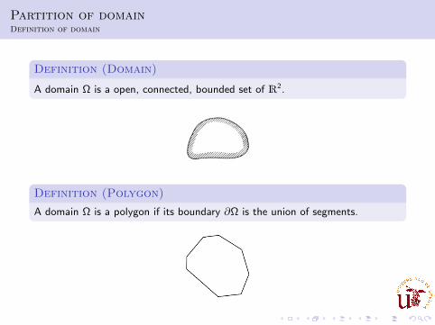
Definition (Domain)

A domain Ω is a open, connected, bounded set of R2.

Definition (Polygon)

A domain Ω is a polygon if its boundary ∂Ω is the union of segments.

Partition of the domainTriangulation

Definition (Element Domain)

An element domain is a connected, compact set of R2 with nonempty interiorand piecewise smooth boundary.

Example

1. A triangle is an element domain.

2. A quadrilateral is an element domain.48 A direct physical approach to problems in elasticity: plane stress

1 2

3

a

b

(a) Triangle (b) Rectangle

1 2

34

a

b

Fig. 2.15 Elements for Problems 2.1 to 2.4.

[viz. Eq. (1.21)] required to transform the nodal degrees of freedom at node 2 and 3 tobe able to impose the boundary conditions.

2.9 A concentrated load, F , is applied to the edge of a two-dimensional plane strain problemas shown in Fig. 2.16(a).(a) Use equilibrium conditions to compute the statically equivalent forces acting at

nodes 1 and 2.(b) Use virtual work to compute the equivalent forces acting on nodes 1 and 2.

2.10 A triangular traction load is applied to the edge of a two-dimensional plane strainproblem as shown in Fig. 2.16(b).(a) Use equilibrium conditions to compute the statically equivalent forces acting at

nodes 1 and 2.(b) Use virtual work to compute the equivalent forces acting on nodes 1 and 2.

2.11 For the rectangular and triangular element shown in Fig. 2.17, compute and assemblethe stiffness matrices associated with nodes 2 and 5 (i.e., K22, K25 and K55). LetE = 1000, ν = 0.25 for the rectangle and E = 1200, ν = 0 for the triangle. Thethickness for the assembly is constant with t = 0.2 cm.

1 2a

(a) Point loading (b) Hydrostatic loading

F

h

1 2

q

a

h

Fig. 2.16 Traction loading on boundary for Problems 2.9 and 2.10.

Partition of the domianTriangulation

Definition (Subdivision)

A subdivision of a domain Ω is a finite collection of element domain ΩiMi=1

such that :

(1) interior Ωi ∩ interior Ωj = ∅ si i 6= j .

(2) Ω = ∪Mi=1Ωi .

Partition of domainTriangulation

Definicion (Triangulation)

A triangulation of a polygon Ω is a subdivision consisting of triangles havingthe property that

(3) no vertex of any triangle lies in the interior of an edge of another triangle.

Remark

Similarly one can define a “quadrilateralation” of a polygonal domain.

Shape Functions and Approximation SpacesConcept of Finite Element

The following definition is due to Ciarlet (1978):

Definition (Finite Element)

Let

1. K ⊂ Rd be a bounded closed set with nonempty interior and piecewisesmooth boundary (the element domain),

2. P(K) be a finite-dimensional space of functions on K (the space of shapefunctions) and

3. N (K) = N1,N2, . . . ,Nk be a basis for P ′ (the set of nodal variables).

Then (K ,P,N ) is called a finite element

Shape Functions and Approximation SpacesLagrange Finite Element

P1-Lagrange Finite Element:

1. Let K be a triangle whose vertexes are denoted by a1, a2, a3.

2. Let P1(K) denote the set of all polynomials in two variables of degree 1,i.e.,

v(x) = a + bx + cy

where a, b, c ∈ R. If follows that λ1, λ2, λ3 ⊂ P1, where

λ1(aj) = δ1j , λ2(aj) = δ2j , λ3(aj) = δ3j ,

is a basis of P1(K) called shape functions.

3. Let N1(K) be a set of evaluation points, i.e., N1(v) = v(a1)N2(v) = v(a2), and N3(v) = v(a3). Theses values are also known as thedegrees of freedom.

Definition

The triplet (K ,P1(K),N1(K)) is called P1-Lagrange Finite Element.

Shape Functions and Approximation SpacesLagrange Finite element

P2-Lagrange Finite Element:

1. Let K be a triangle whose vertexes are denoted by a1, a2, a3, and denotedby a4 = a12, a5 = a13, a6 = a23 the midpoints of the edges of K .

Figure: Vertexes and midpoints of K

Shape Functions and Approximation SpacesLagrange Finite element

2. Let P2(K) denote the set of all polynomials in two variables of degree 1,i.e.,

v(x) = a + bx + cy + dxy + ex2 + fy 2

where a, b, c, d , e, f ∈ R. If follows that λ1, . . . , λ6 ⊂ P2, where

λi (aj) = δij ∀i , j = 1, . . . , 6

is a basis of P2(K) called shape functions.

3. Let N2(K) be a set of evaluation point, i.e., N1(v) = v(a1) N2(v) = v(a2),N3(v) = v(a3), N4(v) = v(a12), N5(v) = v(a13) and N6(v) = v(a23).

Definition

The triplet (K ,P2(K),N2(K)) is called P2-Lagrange Finite Element.

Shape Functions and Approximation SpacesConstructing the approximation space

1 Let Ω ⊂ R2 be a polygonal domain.2 Let Th = K, 0 < h ≤ 1, be a triangulation of Ω, where h = maxK∈Th hK ,

with hk being the diameter of K , i.e., the longest edge of K .3 Let Nh = NjJj=1 be the set of nodes.4 Let (K ,P1(K),N1(K)) be the Lagrange finite element.

Define

X 1h = xh : xh|K ∈ P1(K), ∀K ∈ Th, and xh is continuous at the nodes.

Property

The space X 1h is made of continuos functions on Ω being piecewise linear on K ,

i.e.,X 1

h ⊂ C 0(Ω).

Property

Since we have chosen (K ,P1(K),N1(K)), a function xh ∈ X 1h is determined

only by its value at the nodes. Therefore,

dimX 1h = number of nodes = J.


Choose Vh = X 1h ∩ H1

0 (Ω), i.e.,

Vh = xh : xh|K ∈ P1(K),∀K ∈ Th, and vh = 0 on ∂Ω.

Then a function vh ∈ Vh is determined only by its value at the nodes, exceptthat the nodes on the boundary ∂Ω that vh = 0 and

dimVh = number of interior nodes = M.

Moreover, a basis consists of

ϕi (Nj) =

1 si i = j ,0 si i 6= j .


That is, given vh ∈ Vh, one has

vh(x) =M∑i=1

ηiϕi (x), with ηi = vh(Ni ), ∀x ∈ Ω.

Observe that the support of ϕi (the set of points where ϕi (x) 6= 0) are thetriangles with common vertex Nj .


If one chooses (K ,P2(K),N2(K)) to be the P2-Lagrange finite element, then

X 2h = xh ∈ C 0(Ω) : xh|K ∈ P2(K),∀K ∈ Th

and hence Vh = X 2h ∩ H1

0 (Ω).The basis functions take the form

Figure: Global Shape Functions for P2-Lagrange

Shape Functions and Approximation SpacesAssociated Linear System

FE approximation

Find uh ∈ Vh such that

(∇uh,∇vh) = (f , vh) ∀vh ∈ Vh. (4)

Write uh =∑M

j=1 ξjϕj and take vh = ϕi . Then

M∑j=1

ξj(∇ϕj ,∇ϕi ) = (f , ϕj)

Define A = (aij) y b = (bj) as

aij = (∇ϕj ,∇ϕi ) and bj = (f , ϕi ).

Remark

Solving (4) is equivalent to solving a system of linear equations Aξ = b, whereA (rigid matrix) is a symmetric and positive definite. We thus guaranteeexistence and uniqueness of a solution to (4).

One could also apply the Lax-Milgram theorem to (4) for establishing thewell-posedness.


Example

Consider Ω = [0, 1]× [0, 1] and let Th be a triangulation corresponding to thefollowing figure:

Figure: Triangulation of Ω = [0, 1] × [0, 1]


The associated linear system for P1-Lagrange finite elements is:

4 −1 0 0 · · · 0 −1 0 · · · 0 0−1 4 −1 0 · · · 0 0 −1 · · · 0 0

0 −1 4 −1 · · · 0 0 0 · · · −1 00 0 −1 4 · · · 0 0 0 · · · 0 −1

.

.

.

.

.

.

.

.

.

.

.

.

...

.

.

.

.

.

.

.

.

.

...

.

.

.

.

.

.0 0 0 0 · · · 4 −1 0 · · · 0 0−1 0 0 0 · · · −1 4 −1 · · · 0 0

0 −1 0 0 · · · 0 −1 4 · · · 0 0

.

.

.

.

.

.

.

.

.

.

.

.

...

.

.

.

.

.

.

.

.

.

...

.

.

.

.

.

.0 0 −1 0 · · · 0 0 0 · · · 4 −10 0 0 −1 · · · 0 0 0 · · · −1 4

ξ1ξ2ξ3ξ4

.

.

.

ξM−1ξM

=

b1b2b3b4

.

.

.

bM−1bM

Remark

Any other nodal numbering gives rise to a different matrix A.

Stability and convergence for FEMEnergy norm

Cauchy-Schwarz’ Inequality

Let u, v ∈ L2(Ω). Then(u, v) ≤ ‖u‖‖v‖

Young’s Inequality

Let a, b ≥ 0 and p, q > 0 such that 1p

+ 1q

= 1. Then

ab ≤ 1

2ap +

1

2bq

Poincare’s Inequaltiy)

There exists CΩ > 0 such that(∫Ω

|v |2dx) 1

2

≤ CΩ

(∫Ω

|∇v |2dx) 1

2

∀v ∈ H10 (Ω)

Stability and convergence for FEMEnergy norm

Energy bound

‖∇u‖ ≤ CΩ‖f ‖.

Discrete Energy Bound

‖∇uh‖ ≤ CΩ‖f ‖.

Stability and convergenceError Bounds

We want to study the error u − uh where u is the solution to (2) and uh is thesolution to (3). As Vh ⊂ V , subtracting (3) from (2) for any test function testvh ∈ Vh, we get

(∇(u − uh),∇vh) = 0.

We select vh = u − uh + wh − u with wh ∈ Vh:

(∇(u − uh),∇(u − uh + wh − u)) = 0.

‖∇(u − uh)‖2 = (∇(u − uh),∇(u − wh)).

Applying Cauchy-Schwarz’ and Young’s inequality leads to

Theorem (Cea)

‖∇(u − uh)‖ ≤ infwh∈Vh

‖∇(u − wh)‖.

Stability and ConvergenceError Bounds

Recall

H2(Ω) = u ∈ H1(Ω) :∂2u

∂xj∂xi∈ L2(Ω), i , j = 1, 2.

Let Th = K, 0 < h ≤ 1, a triangulation of Ω, where h = maxK∈Th hK , withhK the diameter of K , i.e., the longest edge of K , and ρK is largest ballcontained in K .

Resultados de interpolacion y consecuencias Resultados generales de caracter local

Caracterısticas geometricas de K y consecuencias (I)

1 hK = maxx ,y2K |x y |: diametro de K2 K = max > 0 : 9B K: grosor de K

Ilustracion para N = 2, K triangular:

Dpto. EDAN, Universidad de Sevilla () Resolucion de EDP 5 / 19Definition

A triangulation Th is said to be regular if there exists a positive constant β suchthat

hKρK≤ β ∀K ∈ Th.


Remark

The regularity condition for Th means geometrically that there cannot betriangles being very flat, i.e., the angles of any triangle K cannot be arbitrarilysmall. The constant β measures how small the triangles of K ∈ Th can be.

Consider NjMj=1 to be the set of interior nodes of Ω and define el nodalinterpolation operator

Πhv =M∑j=1

v(Nj)ϕj

where ϕjMj=1 is a basis of Vh.


Then, if v ∈ H2(Ω) ∩ H10 (Ω) ⊂ C 0(Ω), one has

‖∇(v − Πhv)‖ ≤ Ch‖∇2v‖.

As a consequence, we find:

Theorem (convergence in H10 (Ω))[Cea]

If Ω is a convex polygonal domain:

‖∇(u − uh)‖ ≤ Ch‖∇2u‖.

One can also prove:

Theorem (convergence in L2(Ω))[Aubin-Nitsche]

If Ω is a convex polygonal domain:

‖u − uh‖ ≤ Ch2‖∇2u‖.

partial differential equations: analysis, numerics and control · finite element method: elliptic...

Documents