part vi precise point positioning supported by local ionospheric modeling gs894g
TRANSCRIPT

Part VI
Precise Point Positioning Supported by
Local Ionospheric Modeling
GS894G

Presentation Outline
Research objectives
The Benefits of PPP
MPGPS™ Software
Methodology
Experiments and test results
Summary and Conclusions

Research Objectives
Develop precise point positioning (PPP) methodology and algorithms for surveying and navigation applications
Take advantage of the existing IGS products (precise orbits and clock corrections)
Provide local ionospheric maps (LIM) and tropospheric total zenith delays (TZD) from permanent GPS stations to support single-frequency PPP
Evaluate the quality of single and dual-frequency static and kinematic PPP in post processing

MPGPS™ - Multi Purpose GPS software
Developed at The Ohio State University (OSU)
Positioning Modules Long-range instantaneous (single epoch) RTK GPS Rapid-static Static Multi-station DGPS Precise point positioning (PPP)
Atmospheric Modules Ionosphere modeling and mapping Troposphere modeling
Positioning Solutions Single-baseline Multi-baseline (network) Stand-alone

The Benefits of PPP
Single receiver operation (low-cost)
Can be applied anywhere and anytime under
different dynamics (remote areas, space
applications, etc)
Not limited by baseline length as relative
techniques
Independence on GPS reference stations
Can be applied for static and kinematic platforms

MethodologyError Sources in PPP
Errors affecting the GPS observations Satellite orbit and clock corrections, (provided by IGS)
• accuracy < 5 cm and <0.1 ns (3 cm) Relativistic effects (included in the IGS orbits, except for the
periodic
relativity, which is modeled in MPGPS™)• periodic relativity - up to 30 ns (~9 m)
Receiver and satellite antenna phase center offsets (provided by IGSor NGS)• satellites - up to 1.023 m, receiver up to - 0.2 m
Satellite P1P2 and P1-C1 differential code biases (DCBs) (provided by IGS)• up to 2 ns (0.6 m), accuracy 0.1 ns (3 cm)
Receiver DCB (GPS receiver calibration in MPGPS™ or IGS)• up to 20 ns (6 m), accuracy 0.1 ns (3 cm)
Phase wind-up• up to 1 cycle (~0.2 m) of carrier phase data

MethodologyError Sources in PPP
Errors affecting the GPS observations (cont.) Ionospheric refraction
• Ranges from <1 m to >100 m Tropospheric refraction
• TZD = ~ 2.3 m (for standard atmosphere)
Errors affecting the station coordinates Atmospheric loading
• correction: vertical < 1 cm Ocean loading
• corrections : horizontal < 2 cm, vertical < 5 cm Solid Earth tides
• correction: horizontal < 5 cm, vertical < 30 cm Earth Rotation Parameters, i.e., pole position and UT1-
UTC (included in the IGS orbits)

MethodologyAdjustment Model
bXL
All parameters in the mathematical model are considered
pseudo-observations with a priori information (σ = 0 ÷ )
GLS – Generalized Least Squares adjustment
( , ) 0b bF XF L L 0F F X X FB V B V W
bFL - instantaneous parameters (e.g., ionospheric
delays)- accumulated parameters (e.g., ambiguities)
Two groups of parameters (pseudo-observations) of interest:
Flexibility, easy implementation of:
stochastic constraints fixed constraints weighted parameters filters
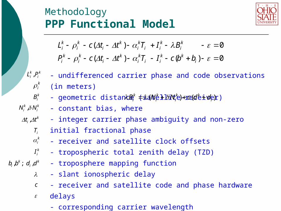
MethodologyPPP Functional Model
( ) 0
( ) ( ) 0
k k k k k ki i i i i i i
k k k k k ki i i i i i i
L c t t T I B
P c t t T I c b b
- undifferenced carrier phase and code observations (in
meters)
- geometric distance (satellite-receiver)
- constant bias, where
- integer carrier phase ambiguity and non-zero initial fractional
phase
- receiver and satellite clock offsets
- tropospheric total zenith delay (TZD)
- troposphere mapping function
- slant ionospheric delay
- receiver and satellite code and phase hardware delays
- corresponding carrier wavelength
- speed of light
- random error or residual
( ) ( )k k k ki i i iB N N c d d
,k ki iN N
,k ki iL P
, kit t
iTkikiI
, ; ,k ki ib b d d
c
kiB
ki

MethodologyPPP - Functional Model Unknowns
Permanent GPS station solution for local ionosphere maps (LIM)
receiver clock tropospheric TZD slant ionospheric delays bias parameters (non-integer ambiguities and hardware
delays) Single-frequency positioning solution
rover coordinates receiver clock bias parameters
Dual-frequency (ionosphere-free) positioning solution
rover coordinates receiver clock tropospheric TZD bias parameters

Methodology Local Ionospheric Model (LIM)
Supports PPP in case of single-frequency receiver
Single layer model (SLM) ionosphere approximation
Slant ionospheric delays estimation from dual-frequency GPS data at the neighboring permanent stations
Slant ionospheric delays conversion to vertical total electron content (VTEC) at ionosphere pierce points (IPPs)
Kriging interpolation to produce LIM in a form of a grid using the calculated vertical TEC values at IPPs
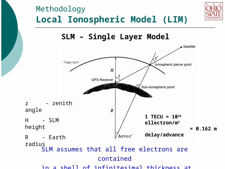
SLM assumes that all free electrons are contained
in a shell of infinitesimal thickness at altitude H
z - zenith angle
H - SLM height
R - Earth radius
SLM – Single Layer Model
Methodology Local Ionospheric Model (LIM)
1 TECU = 1016 ellectron/m2
= 0.162 m delay/advance

Methodology PPP Models
Three PPP MPGPS™ models were tested in post processing mode Static PPP – dual-frequency (ionosphere-free)
Static PPP – single-frequency supported by LIM
Kinematic PPP – single-frequency supported by LIM
Adaptive filter for kinematic solution Follows the dynamic variations of the system
estimates and stochastic models
Propagates the coordinate and ionosphere residuals together with their stochastic characteristics
Forward and backward filters

Experiments and test resultsData Source
Four stations, IGS/EPN (EUREF permanent network)
Three stations were used to derive LIM and TZD (BOR1, GOPE, KRAW)
One station was selected as a rover (WROC)
Two three-hour sessions
01 - 04 UTC (nighttime - lowest TEC level)
13 - 17 UTC (daytime - highest TEC level)
30-second sampling rate (i.e., 360 epochs per session)
Phase-smoothed pseudoranges
Distances between permanent stations ~330 km (average)
Distances to the rover ~130–230 km

Experiments and test results
Test Area Map
Czech Republic
Poland
- LIM/TZD
- PPP (rover)
N
____________________________________________________
Rover

Experiments and test resultsSatellite Geometry - Station WROC
01-04 UTC nighttime
4-7 satellites
13-17 UTC daytime
4-5 satellites
Poor satellite geometry, high GDOP - usually over 5
A short period with very poor geometry occurred in both sessions
50 100 150 200 250 300 3503
4
5
6
7
8
No.
of s
at.
50 100 150 200 250 300 3500
5
10
15
20
Epochs
GD
OP
50 100 150 200 250 300 3503
4
5
6
7
8
No.
of s
at.
50 100 150 200 250 300 3500
5
10
15
20
Epochs
GD
OP
____________________________________________________
GDOP = ~80
GDOP =~1000

Experiments and test resultsExample LIM-derived ionospheric delays
0 50 100 150 200 250 300 3500
1
2
3
4
5
6
7
Epochs
[m]
PRN 15PRN 16PRN 18PRN 23PRN 31PRN 14PRN 11PRN 3
0 50 100 150 200 250 300 3500
1
2
3
4
5
6
7
Epochs
[m]
PRN 8PRN 27PRN 28PRN 29PRN 26PRN 9
Station WROC (rover)
01-04 UTC nighttime
lowest TEC
13-17 UTC daytime
highest TEC
_______________________________________________________

Experiments and test resultsStatic PPP Analysis – Station WROC
50 100 150 200 250 300 350-1
-0.8
-0.6
-0.4
-0.2
0
0.2
0.4
0.6
0.8
1
Epochs
[m]
neu
50 100 150 200 250 300 350-1
-0.8
-0.6
-0.4
-0.2
0
0.2
0.4
0.6
0.8
1Static ion-free
neu
Epochs
[m]
50 100 150 200 250 300 350-1
-0.8
-0.6
-0.4
-0.2
0
0.2
0.4
0.6
0.8
1
Epochs
[m]
neu
50 100 150 200 250 300 350-1
-0.8
-0.6
-0.4
-0.2
0
0.2
0.4
0.6
0.8
1neu
[m]
Epochs
Nighttime, dual-frequency(ionosphere-free LC)
Daytime, dual-frequency(ionosphere-free LC)
Nighttime, single-frequencysupported by LIM
Daytime, single-frequencysupported by LIM
____________________________________________________

Experiments and test resultsStatic PPP Analysis – Station WROC
Ionosphere-free solution Horizontal - sub-decimeter-level position accuracy Vertical - decimeter-level Nighttime - convergence after 40 minutes Daytime - convergence after 25 minutes
Single-frequency solution supported by
LIM Good agreement with its ionosphere-free counterpart Similar accuracies and convergence times LIM proved to be efficient in removing the ionospheric
delays

Experiments and test resultsKinematic PPP Analysis – Station WROC
01-04 UTC (nighttime) 13-17 UTC (daytime)
Unfiltered single-
frequencysupported by
LIM
Filteredsingle-
frequencysupported by
LIM
50 100 150 200 250 300 350-1
-0.8
-0.6
-0.4
-0.2
0
0.2
0.4
0.6
0.8
1
Epochs
[m]
neu
50 100 150 200 250 300 350-1
-0.8
-0.6
-0.4
-0.2
0
0.2
0.4
0.6
0.8
1neu
[m]
Epochs
50 100 150 200 250 300 350-1
-0.8
-0.6
-0.4
-0.2
0
0.2
0.4
0.6
0.8
1
Epochs
[m]
nee
50 100 150 200 250 300 350-1
-0.8
-0.6
-0.4
-0.2
0
0.2
0.4
0.6
0.8
1neu
[m]
Epochs
____________________________________________________

The unfiltered solutions are very noisy in both sessions
In the filtered solution the large residuals were smoothed out after a few iterations (3-4)
The filtered kinematic solutions show similar accuracies as obtained in the static case
Sub-decimeter horizontal and decimeter-level vertical position accuracy was achieved
Experiments and test resultsKinematic PPP Analysis – Station WROC

Summary and Conclusions
The sequential GLS adjustment was successfully applied in
the PPP algorithm
Single-frequency static and kinematic PPP solutions,
supported by LIM, are comparable to the ionosphere-free
solutions
The results prove a good quality of the obtained LIM
The effectiveness of the adaptive filter was presented in the
kinematic mode, even under unfavorable satellite geometry
This algorithm may be applied in geodetic applications,
where sub-decimeter level accuracy is required