Part III Differential GeometryLecture Notes

Mihalis Dafermos

Contents

1 Introduction 3

1.1 From smooth surfaces to smooth manifolds . . . . . . . . . . . . 31.2 What defines geometry? . . . . . . . . . . . . . . . . . . . . . . . 51.3 Geometry, curvature, topology . . . . . . . . . . . . . . . . . . . 7

1.3.1 Aside: Hyperbolic space and non-euclidean geometry . . . 81.4 General relativity . . . . . . . . . . . . . . . . . . . . . . . . . . . 8

2 Manifolds 9

2.1 Basic definitions . . . . . . . . . . . . . . . . . . . . . . . . . . . 92.1.1 Charts and atlases . . . . . . . . . . . . . . . . . . . . . . 92.1.2 Definition of smooth manifold . . . . . . . . . . . . . . . . 102.1.3 Smooth maps of manifolds . . . . . . . . . . . . . . . . . . 102.1.4 Examples . . . . . . . . . . . . . . . . . . . . . . . . . . . 11

2.2 Tangent vectors . . . . . . . . . . . . . . . . . . . . . . . . . . . . 122.3 The tangent bundle . . . . . . . . . . . . . . . . . . . . . . . . . . 13

3 More bundles 14

3.1 The general definition of vector bundle . . . . . . . . . . . . . . . 143.2 Dual bundles and the cotangent bundle . . . . . . . . . . . . . . 153.3 The pull-back and the push forward . . . . . . . . . . . . . . . . 153.4 Multilinear algebra . . . . . . . . . . . . . . . . . . . . . . . . . . 163.5 Tensor bundles . . . . . . . . . . . . . . . . . . . . . . . . . . . . 17

4 Riemannian manifolds 18

4.1 Examples . . . . . . . . . . . . . . . . . . . . . . . . . . . . . . . 194.2 Construction of Riemannian metrics . . . . . . . . . . . . . . . . 19

4.2.1 Overkill . . . . . . . . . . . . . . . . . . . . . . . . . . . . 194.2.2 Construction via partition of unity . . . . . . . . . . . . . 19

4.3 The semi-Riemannian case . . . . . . . . . . . . . . . . . . . . . . 204.4 Topologists vs. geometers . . . . . . . . . . . . . . . . . . . . . . 204.5 Isometry . . . . . . . . . . . . . . . . . . . . . . . . . . . . . . . . 21

5 Vector fields and O.D.E.’s 22

5.1 Existence of integral curves . . . . . . . . . . . . . . . . . . . . . 225.2 Smooth dependence on initial data; 1-parameter groups of trans-

formations . . . . . . . . . . . . . . . . . . . . . . . . . . . . . . . 235.3 The Lie bracket . . . . . . . . . . . . . . . . . . . . . . . . . . . . 235.4 Lie differentiation . . . . . . . . . . . . . . . . . . . . . . . . . . . 25

1

6 Connections 25

6.1 Geodesics and parallelism in Rn . . . . . . . . . . . . . . . . . . . 266.2 Connection in a vector bundle . . . . . . . . . . . . . . . . . . . . 28

6.2.1 Γijk is not a tensor! . . . . . . . . . . . . . . . . . . . . . . 296.3 The Levi-Civita connection . . . . . . . . . . . . . . . . . . . . . 29

6.3.1 The Levi–Civita connection in local coordinates . . . . . . 296.3.2 Aside: raising and lowering indices with the metric . . . . 30

7 Geodesics and parallel transport 30

7.1 The definition of geodesic . . . . . . . . . . . . . . . . . . . . . . 307.2 The first variation formula . . . . . . . . . . . . . . . . . . . . . . 317.3 Parallel transport . . . . . . . . . . . . . . . . . . . . . . . . . . . 337.4 Existence of geodesics . . . . . . . . . . . . . . . . . . . . . . . . 34

8 The exponential map 34

8.1 The differential of exp . . . . . . . . . . . . . . . . . . . . . . . . 358.2 The Gauss lemma . . . . . . . . . . . . . . . . . . . . . . . . . . 368.3 Geodesically convex neighbourhoods . . . . . . . . . . . . . . . . 388.4 Application: length minimizing curves are geodesics . . . . . . . 39

9 Geodesic completeness and the Hopf-Rinow theorem 40

9.1 The metric space structure . . . . . . . . . . . . . . . . . . . . . 409.2 Hopf–Rinow theorem . . . . . . . . . . . . . . . . . . . . . . . . . 40

10 The second variation 42

11 The curvature tensor 44

11.1 Ricci and scalar curvature . . . . . . . . . . . . . . . . . . . . . . 4411.2 Sectional curvature . . . . . . . . . . . . . . . . . . . . . . . . . . 4511.3 Curvature in local coordinates . . . . . . . . . . . . . . . . . . . . 4611.4 Curvature as a local isometry invariant . . . . . . . . . . . . . . . 4611.5 Spaces of constant curvature . . . . . . . . . . . . . . . . . . . . 47

11.5.1 Rn . . . . . . . . . . . . . . . . . . . . . . . . . . . . . . . 4711.5.2 Sn . . . . . . . . . . . . . . . . . . . . . . . . . . . . . . . 4711.5.3 Hn . . . . . . . . . . . . . . . . . . . . . . . . . . . . . . . 47

12 Simple comparison theorems 48

12.1 Bonnet–Myers theorem . . . . . . . . . . . . . . . . . . . . . . . . 4812.2 Synge’s theorem . . . . . . . . . . . . . . . . . . . . . . . . . . . 4912.3 Cartan–Hadamard theorem . . . . . . . . . . . . . . . . . . . . . 49

13 Jacobi fields 49

13.1 The index form I(V,W ) . . . . . . . . . . . . . . . . . . . . . . . 5013.2 Conjugate points and the index form . . . . . . . . . . . . . . . . 5113.3 The use of Jacobi fields . . . . . . . . . . . . . . . . . . . . . . . 52

14 Lorentzian geometry and Penrose’s incompleteness theorem 53

14.1 Timelike, null, and spacelike . . . . . . . . . . . . . . . . . . . . . 5314.1.1 Vectors and vector fields . . . . . . . . . . . . . . . . . . . 5314.1.2 Curves . . . . . . . . . . . . . . . . . . . . . . . . . . . . . 5314.1.3 Submanifolds . . . . . . . . . . . . . . . . . . . . . . . . . 53

2

14.2 Time orientation and causal structure . . . . . . . . . . . . . . . 5414.3 Global hyperbolicity . . . . . . . . . . . . . . . . . . . . . . . . . 5414.4 Closed trapped 2-surfaces . . . . . . . . . . . . . . . . . . . . . . 5414.5 Statement of Penrose’s theorem . . . . . . . . . . . . . . . . . . . 5414.6 Sketch of the proof . . . . . . . . . . . . . . . . . . . . . . . . . . 5414.7 Examples . . . . . . . . . . . . . . . . . . . . . . . . . . . . . . . 54

14.7.1 Schwarzschild . . . . . . . . . . . . . . . . . . . . . . . . . 5414.7.2 Reissner-Nordstrom . . . . . . . . . . . . . . . . . . . . . 54

15 Appendix: Differential forms and Cartan’s method 54

16 Guide to the literature 54

16.1 Foundations of smooth manifolds, bundles, connections . . . . . . 5516.2 Riemannian geometry . . . . . . . . . . . . . . . . . . . . . . . . 5516.3 General relativity . . . . . . . . . . . . . . . . . . . . . . . . . . . 56

1 Introduction

These notes accompany my Michaelmas 2012 Cambridge Part III course on Dif-ferential geometry. The purpose of the course is to cover the basics of differentialmanifolds and elementary Riemannian geometry, up to and including some easycomparison theorems. Time permitting, Penrose’s incompleteness theorems ofgeneral relativity will also be discussed.

We will give the formal definition of manifold in Section 2. In the rest ofthis introduction, we first discuss informally how the manifold concept naturallyarises from abstracting precisely that structure on smooth surfaces in Euclideanspace that allows us to define consistently smooth functions. We will then give apreliminary sketch of the notion of Riemannian metric first in two then in higherdimensions and give a brief overview of some of the main themes of Riemanniangeometry to follow later in the course.

These notes are still very much “under construction”. Moreover, they areon the whole pretty informal and meant as a companion but not a substitutefor a careful and detailed textbook treatment of the material–for the latter, thereader should consult the references described in Section 16.

1.1 From smooth surfaces to smooth manifolds

The simplest way that the objects of the form we call smooth surfaces S ⊂ E3

arise are as level sets of a smooth function, say f(x, y, z) = c, at a non-critical1

value c. Example: S2 as x2 + y2 + z2 = 1. It is the implicit function theorem2

that says that these objects are, in some sense, two dimensional, i.e. that S canbe expressed as the union of the images of a collection of maps ψα : Vα → E3,Vα ⊂ E2, such that ψα is smooth, Dψα is one-to-one, and denoting ψα(Vα) as

1i.e. a value c ∈ R such that df(p) is surjective for all p ∈ f−1(c)2The reader is assumed familiar with standard results in multivariable analysis.

3

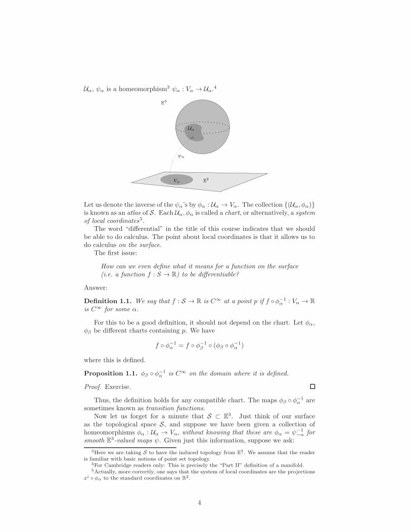
Uα, ψα is a homeomorphism3 ψα : Vα → Uα.4

ψα

E2

E3

Uα

Vα

Let us denote the inverse of the ψα’s by φα : Uα → Vα. The collection {(Uα, φα)}is known as an atlas of S. Each Uα, φα is called a chart, or alternatively, a systemof local coordinates5.

The word “differential” in the title of this course indicates that we shouldbe able to do calculus. The point about local coordinates is that it allows us todo calculus on the surface.

The first issue:

How can we even define what it means for a function on the surface(i.e. a function f : S → R) to be differentiable?

Answer:

Definition 1.1. We say that f : S → R is C∞ at a point p if f ◦φ−1α : Vα → R

is C∞ for some α.

For this to be a good definition, it should not depend on the chart. Let φα,φβ be different charts containing p. We have

f ◦ φ−1α = f ◦ φ−1

β ◦ (φβ ◦ φ−1α )

where this is defined.

Proposition 1.1. φβ ◦ φ−1α is C∞ on the domain where it is defined.

Proof. Exercise.

Thus, the definition holds for any compatible chart. The maps φβ ◦ φ−1α are

sometimes known as transition functions.Now let us forget for a minute that S ⊂ E3. Just think of our surface

as the topological space S, and suppose we have been given a collection ofhomeomorphisms φα : Uα → Vα, without knowing that these are φα = ψ−1

−α forsmooth E3-valued maps ψ. Given just this information, suppose we ask:

3Here we are taking S to have the induced topology from E3. We assume that the readeris familiar with basic notions of point set topology.

4For Cambridge readers only: This is precisely the “Part II” definition of a manifold.5Actually, more correctly, one says that the system of local coordinates are the projections

xi ◦ φα to the standard coordinates on R2.

4

What is the least amount of structure necessary to define consistentlythe notion that a function f : S → R is smooth?

We easily see that the definition provided by Definition 1.1 is a good def-inition provided that the result of Proposition 1.1 happens to hold. For it isprecisely the statement of the latter proposition which shows that if φ ◦ φ−1

α issmooth at p for some α where Uα contains p, then it is smooth for all charts.

We now apply one of the oldest tricks of mathematical abstraction. Wemake a proposition into a definition. The notion of an abstract smooth surfacedistills the property embodied by Proposition 1.1 from that of a surface in E3,and builds it into the definition.

Definition 1.2. An abstract smooth surface is a topological space S togetherwith an open cover Uα and homeomorphisms φα : Uα → Vα, with Vα opensubsets of R2, such that φβ ◦ φ−1

α , where defined, are C∞.

The notion of a smooth n-dimensional manifoldM is defined now preciselyas above, where R2 is replaced by Rn.6

Definition 1.3. A map f : M → M is smooth if φβ ◦ f ◦ φ−1α is smooth for

some α, β.

Check that this is a good definition (i.e. “for some” implies “for all”).

Definition 1.4. M and M are said to be diffeomorphic if there exists anf :M→ M such that f and f−1 are both smooth.

Exercise: The dimension n of a manifold is uniquely defined and a diffeomor-phism invariant.

Examples: En, Sn, products, quotients, twisted products (fiber bundles,etc.), connected sums, configuration spaces from classical mechanics. The pointis that manifolds are a very flexible category and there is the usual economyprovided by a good definition. We will discuss all this soon enough in the course.

1.2 What defines geometry?

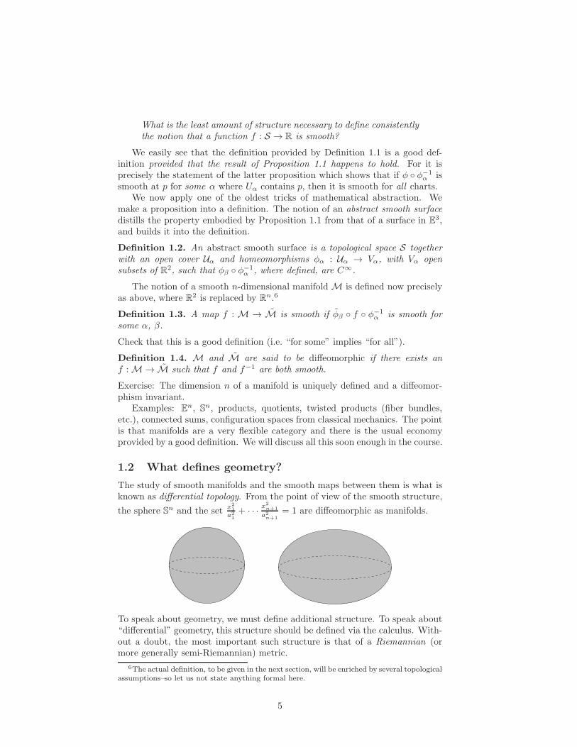
The study of smooth manifolds and the smooth maps between them is what isknown as differential topology. From the point of view of the smooth structure,

the sphere Sn and the setx21

a21+ · · · x

2n+1

a2n+1= 1 are diffeomorphic as manifolds.

To speak about geometry, we must define additional structure. To speak about“differential” geometry, this structure should be defined via the calculus. With-out a doubt, the most important such structure is that of a Riemannian (ormore generally semi-Riemannian) metric.

6The actual definition, to be given in the next section, will be enriched by several topologicalassumptions–so let us not state anything formal here.

5

This concept again arises from distilling from the theory of surfaces in E3 apiece of structure: A surface S ⊂ E3 comes with a notion of how to measurethe lengths of curves. This notion can be characterized at the differential level.Formally, we may write

dx2 + dy2 + dz2 = E(u, v)du2 + 2F (u, v)dudv +G(u, v)dv2, (1)

where

E =

(∂x

∂u

)2

+

(∂y

∂u

)2

+

(∂z

∂u

)2

F =∂x

∂u

∂x

∂v+∂y

∂u

∂y

∂v+∂z

∂u

∂z

∂v

G =

(∂x

∂v

)2

+

(∂y

∂v

)2

+

(∂z

∂v

)2

.

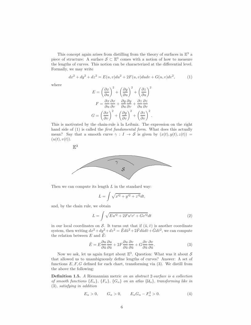
This is motivated by the chain-rule a la Leibniz. The expression on the righthand side of (1) is called the first fundamental form. What does this actuallymean? Say that a smooth curve γ : I → S is given by (x(t), y(t), z(t)) =(u(t), v(t)).

Sγ

E3

Then we can compute its length L in the standard way:

L =

∫ √x′2 + y′2 + z′2dt,

and, by the chain rule, we obtain

L =

∫ √Eu′2 + 2Fu′v′ +Gv′2dt (2)

in our local coordinates on S. It turns out that if (u, v) is another coordinatesystem, then writing dx2+dy2+dz2 = Edu2+2F dudv+Gdv2, we can computethe relation between E and E:

E = E∂u

∂u

∂u

∂u+ 2F

∂u

∂u

∂v

∂u+G

∂v

∂u

∂v

∂u. (3)

Now we ask, let us again forget about E3. Question: What was it about Sthat allowed us to unambiguously define lengths of curves? Answer: A set offunctions E,F,G defined for each chart, transforming via (3). We distill fromthe above the following:

Definition 1.5. A Riemannian metric on an abstract 2-surface is a collectionof smooth functions {Eα}, {Fα}, {Gα} on an atlas {Uα}, transforming like in(3), satisfying in addition

Eα > 0, Gα > 0, EαGα − F 2α > 0. (4)

6

In particular, the formula (2) now allows one to define consistently the notionof the length of a smooth curve φ : I → S.7 The condition (4) ensures that ournotion of length is positive.8

The expression on the right hand side can be generalized to n dimensions,and this defines the notion of a Riemannian metric on a smooth manifold.9 Acouple

(M, g)

consisting of an n-dimensional manifoldM, together with a Riemannian metricg defined onM, is known as a Riemannian manifold. Riemannian geometry isthe study of Riemannian manifolds.

The reader familiar with the geometry of surfaces has no doubt encoun-tered the so-called Theorema Egregium of Gauss. This says that the curvature,originally, defined using the so-called second fundamental form10, in fact canbe expressed as a complicated expression in local coordinates involving up tosecond derivatives of the compontents E, F , G of the first fundamental form.That is to say, it could have been defined in the first place as said expression.In particular, the notion of curvature can thus be defined for abstract surfaces.One main difficulty in Riemannian geometry in higher dimensions is the alge-braic complexity of the analogue of this curvature curvature, which is no-longera scalar, but a so-called “tensor”.

1.3 Geometry, curvature, topology

The following remarks are meant to give a taste of the kinds of results one wantsto prove in geometry. Some familiarity with curvature of surfaces will be usefulfor getting a sense of what these statements mean.

The common thread in these examples is that they relate completeness,curvature and global behaviour (e.g. topology):

Theorem 1.1 (Hadamard–Cartan). Let (M, g) be a simply-connected11 n-dimensional complete Riemannian manifold with nonpositive “sectional curva-ture”. Then (M, g) is diffeomorphic to Rn.

Theorem 1.2 (Synge). Let (M, g) be complete, orientable, even-dimensionaland of positive “sectional curvature”. Then (M, g) is simply connected.

Theorem 1.3 (Bonnet–Myers). Let (M, g) be a complete n-dimensional, n ≥ 2,manifold whose “Ricci curvature” satisfies

Ric ≥ (n− 1)kg

for some k > 0. Then the diameter ofM satisfies

diam(M) ≤ π/√k.

7How to define a smooth curve?8The semi-Riemannian case replaces (4) with the assumption that this determinant is

non-zero. See Section 1.4.9As we have tentatively defined them, not all manifolds admit Riemannian metrics. But

Hausdorff paracompact ones do. . .10For those who know about the geometry of curves and surfaces. . .11We will often make reference to basic notions of algebraic topology.

7

1.3.1 Aside: Hyperbolic space and non-euclidean geometry

The set H2 can be covered by one chart {(u, v) : v > 0}, and the Riemannianmetric is given by

1

v2(du2 + dv2). (5)

Later on we will recognize H2 as a complete space form with the topology ofR2 and with constant curvature −1. This defines a so-called non-Euclideangeometry, a geometry satisfying all the axioms of Euclid with the exceptionof the so-called fifth postulate. In particular, the existence of the Riemanniangeometry (5) shows the necessity of the Euclidean fifth postulate to determineEuclidean geometry.

The enigma of why it took so long for this to be understood is in partexplained by the following global theorem:

Theorem 1.4. Let (S, g) be an abstract surface with Riemannian metric. If Sis complete with constant negative curvature, then S cannot arise as a subset ofE3 so that g is induced as in (1) (in fact, not even as an immersed surface.)

Compare this with the case of the sphere.

1.4 General relativity

A subject with great formal similarity, but a somewhat diverging epistomologicalbasis, with Riemannian geometry is “general relativity”. The basis for thistheory is a four dimensional manifold: M, called spacetime, together with a so-called Lorentzian metric, i.e. a smooth quadratic form

∑gijdx

idxj such that thesignature of g is (−,+,+,+). (In two dimensions, Lorentzian vs. Riemannianwould just mean that the sign of (4) is flipped.) Pure Lorentzian geometryin full generality is more complicated and less studied than pure Riemanniangeometry. What sets general relativity apart from pure geometry, is that in thistheory, the Lorentzian metric must satisfy a set of partial differential equations,the so-called Einstein equations. These equations constitute a relation betweena geometric quantity, the Einstein tensor12, and the energy-momentum contentof matter. In the case where there is no matter present, these equations takethe form

Ric = 0

The central questions in general relativity are questions of the dynamics of thissystem. It is thus a much more rigid subject.

The above comments notwithstanding, there are (quite surprisingly!) somespectacular theorems in general relativity which can be proven via pure geom-etry. The reason: When the dynamics of matter is not specified, the Einsteinequations still yield inequalities for this curvature tensor, analogous in manyways to the inequalities in the statement of the previous theorems. This allowsone to prove so-called singularity theorems–better termed, the incompletenesstheorems, the most important of which is the following result of Penrose

Theorem 1.5 (Penrose, 1965). Let (M, g) be a globally hyperbolic Lorentzian4-manifold with non-compact Cauchy hyper surface satisfying

Ric(V, V ) ≥ 0

12This is an expression derived from the Ricci and scalar curvatures.

8

for all null vectors V . Suppose moreover that (M, g) contains a closed trapped2-surface. Then (M, g) is future-causally geodesically complete.

This theorem can be directly compared to the Bonnet–Myers theorem re-ferred to before. The elements entering into the proof are actually more orless the same, but the traditional logical sequence of their statements different.Whereas Bonnet–Myers is phrased

completenessmild topological assumption,

Ricci curvature sign⇒ diameter bound

Penrose’s theorem is traditionally phrased:

mild geometric/topological assumption,Ricci curvature sign,∃trapped surface

⇒ incompleteness

The similarity to Bonnet–Myers is more clear if we phrase Penrose’s theoremequivalently

completenesslessmild geometric/topological assumption,

Ricci curvature sign,∃trapped surface

⇒ Cauchy hypersurface is compact

Time permitting, we will discuss these later. . .

2 Manifolds

2.1 Basic definitions

2.1.1 Charts and atlases

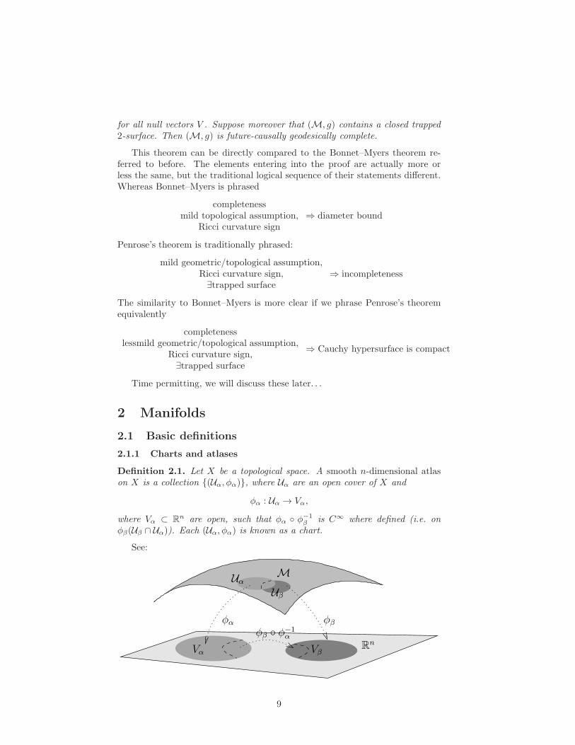
Definition 2.1. Let X be a topological space. A smooth n-dimensional atlason X is a collection {(Uα, φα)}, where Uα are an open cover of X and

φα : Uα → Vα,

where Vα ⊂ Rn are open, such that φα ◦ φ−1β is C∞ where defined (i.e. on

φβ(Uβ ∩ Uα)). Each (Uα, φα) is known as a chart.

See:

M

φα φβ

RnVβVα

φβ ◦ φ−1α

UαUβ

9

Note that φα ◦φ−1β is a map from an open subset of Rn to Rn, so it makes sense

to discuss it’s smoothness!Let X be a topological space and {(Uα, φα)} a smooth atlas. Let (U , φ) be

such that U ⊂ X is open, φ : U → V ⊂ Rn a homeomorphism, such that

φ ◦ φ−1α , φα ◦ φ−1 are C∞ where defined. (6)

Then {(Uα, φα)} ∪ {(U , φ)} is again an atlas.

Definition 2.2. Let X be a topological space and {(Uα, φα)} a smooth atlas.{(Uα, φα)} is maximal if for all (U , φ) as above satisfying (6), then (U , φ) ∈{(Uα, φα)}.

One can easily show

Proposition 2.1. Given an atlas on X, there is a unique maximal atlas con-taining it.

Given an atlas {(Uα, φα}, the restriction of φα to all open U ⊂ Uα will inparticular be in the maximal atlas containing {(Uα, φα)}.

2.1.2 Definition of smooth manifold

Definition 2.3. A C∞ manifold of dimension n is a Hausdorff, second count-able and paracompact topological space M, together with maximal smooth n-dimensional atlas.

Given a chart (Uα, φα), we call πi ◦ φα a system of local coordinates, whereπi denote the projections to standard coordinates on Rn. Very often in notationwe completely suppress φα and talk about local coordinates (x1, . . . , xn). It isunderstood that x1 = π1 ◦ φα for a φα.

2.1.3 Smooth maps of manifolds

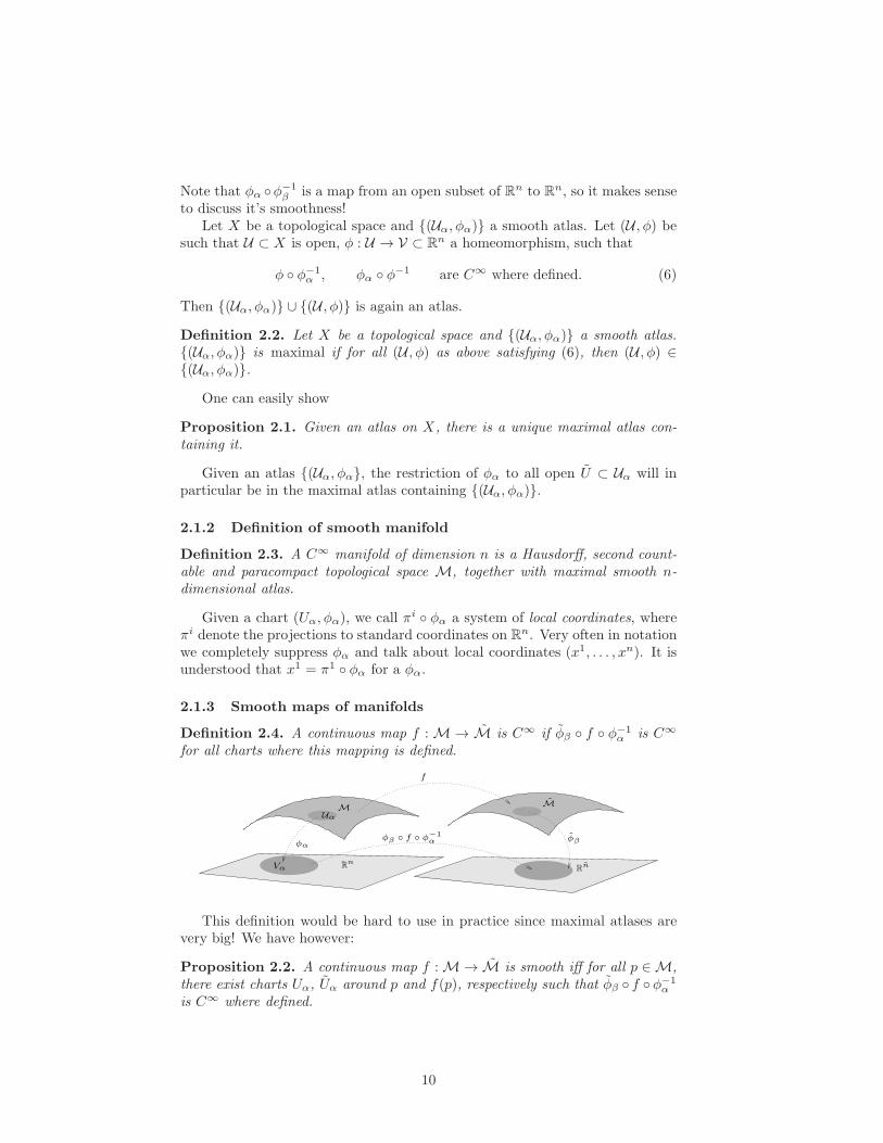
Definition 2.4. A continuous map f :M→ M is C∞ if φβ ◦ f ◦ φ−1α is C∞

for all charts where this mapping is defined.

M

φα

M

Rn

Rn

φβ

Vα

φβ ◦ f ◦ φ−1α

f

Uα

This definition would be hard to use in practice since maximal atlases arevery big! We have however:

Proposition 2.2. A continuous map f :M→ M is smooth iff for all p ∈M,there exist charts Uα, Uα around p and f(p), respectively such that φβ ◦ f ◦ φ−1

α

is C∞ where defined.

10

This follows immediately from the smoothness of the transition functions.As we said already in the introduction, this is the whole point of the definitionof manifolds: it allows us to talk about smooth functions (and more generallysmooth maps) by checking smoothness with respect to a particular choice ofcharts.

IfM and M are of dimensions m and n respectively we shall often refer ton coordinate components of the map

φ−1α ◦ f ◦ φβ

byf1(x1, x2, . . . , xm), . . . , fn(x1, . . . , xm).

With this notation, the map f :M→ M is smooth iff the above maps f i aresmooth in some choice of local coordinates around every point.

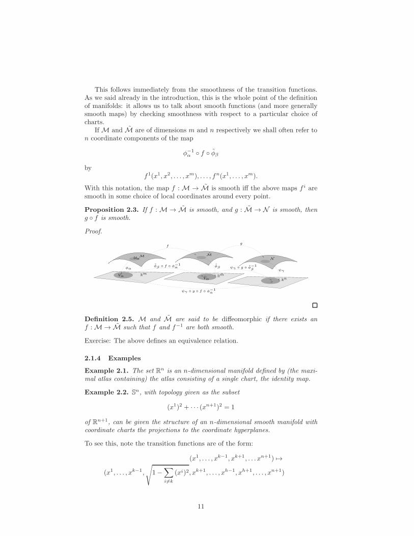
Proposition 2.3. If f :M→ M is smooth, and g : M → N is smooth, theng ◦ f is smooth.

Proof.

M

φα

Rm

N

Rn

ψγ

M

Rm

φβ

Vα

φβ ◦ f ◦ φ−1α

g

ψγ ◦ g ◦ φ−1β

f

ψγ ◦ g ◦ f ◦ φ−1α

Vα

Uα

Definition 2.5. M and M are said to be diffeomorphic if there exists anf :M→ M such that f and f−1 are both smooth.

Exercise: The above defines an equivalence relation.

2.1.4 Examples

Example 2.1. The set Rn is an n-dimensional manifold defined by (the maxi-mal atlas containing) the atlas consisting of a single chart, the identity map.

Example 2.2. Sn, with topology given as the subset

(x1)2 + · · · (xn+1)2 = 1

of Rn+1, can be given the structure of an n-dimensional smooth manifold withcoordinate charts the projections to the coordinate hyperplanes.

To see this, note the transition functions are of the form:

(x1, . . . , xk−1, xk+1, . . . xn+1) 7→

(x1, . . . , xk−1,

√1−

∑

i6=k

(xi)2, xk+1, . . . , xh−1, xh+1, . . . , xn+1)

11

Note. In various dimensions, for instance 7 and (conjecturally) 4, there aredifferentiable structures inequivalent to the above13 which live on the sametopology. These are called exotic spheres.

Example 2.3. Denote by RPn the set of all lines through the origin in n+ 1-dimensional space. This space can be endowed with the structure of an n-dimensional manifold, and is then called real projective space. With this struc-ture the map π : Sn → RPn is smooth.

This is an example of the quotient by a discrete group action. For an exten-sion of this kind of construction, see the first example sheet.

Example 2.4. Let M and N be manifolds. Then one can define a naturalmanifold structure on M×N .

Take {(Uα × Uβ, φα × φβ)}. Complete the details. . .

2.2 Tangent vectors

LetM be a smooth manifold, let p ∈M. Let X(p) denote the algebra of locallyC∞ functions at p.14 Note that if f ∈ X(p) and g ∈ X(p) then fg ∈ X(p),where fg is a locally defined function.

Definition 2.6. A derivation D at p is a mapping D : X(p) → R satisfy-ing D(λf + µg) = λDf + µDg, for λ, µ scalars, and, in addition, D(fg) =(Df)g(p) + f(p)(Dg).

Proposition 2.4. The set of derivations at p define a vector space of dimensionn, denoted TpM.

Proof. The fact that TpM is a vector space is clear. Let xi be a system of localcoordinates centred at p. Define a map ∂

∂xi |p by

∂

∂xi|pf = ∂xif ◦ φ−1

α |φα(p)

where φα is the name of the chart map defining the coordinates xi. (Note∂∂xi |pxj ◦ φα = δji . This in particular implies that the ∂

∂xi are linearly inde-

pendent.) Clearly ∂∂xi |p is a derivation, by the well-known properties of deriva-

tives. We want to show that the{

∂∂xi

∣∣p} span TpM. It suffices to show that

if Dxi ◦ φα = 0 for all xi, then D = 0. So let D be such a D, and let f bearbitrary. Locally, f = αix

i + gixi where αi ∈ R and where gi are C

∞. Thus,Df(p) = αiDx

i + xiDgi = 0, since WLOG we can choose p to correspond to

the origin of coordinates.

Note. We have used above the Einstein summation convention, i.e. the conven-tion that whenever we the same index “up” and “down”, as in the expressionαix

i, we are to understand∑n

i=1 αixi. Note that the index i of ∂

∂xi |p is to beunderstood as down. Here n = dimM.

Definition 2.7. We will call TpM the tangent space of M at p, and we willcall its elements tangent vectors.

13i.e. such that the resulting manifold is not diffeomeorphic to the above14Exercise: define this space formally in whatever way you choose.

12

Proposition 2.5. Let xi and xi denote two coordinate systems. Then ∂∂xi |p =

∂xj

∂xi∂∂xj |p, for all p in the common domain of the two coordinate charts.

Proof. If we apply an arbitrary f to both sides, then by the chain rule, the leftand right hand side coincide. Thus, the two expressions correspond to one andthe same derivation.

Notation. In writing ∂xj

∂xi one is to understand ∂i(πj ◦ φ ◦ φ−1), where φ and φ

are the two charts corresponding to the local coordinates.15

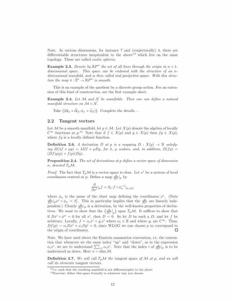
The geometric interpretation of derivations at p: Let γ be a smooth curvethrough p, i.e. a smooth map γ : (−ǫ, ǫ) → M such that γ(0) = p. Given f ,define a derivation Dγ at p by Dγf = (f ◦ γ)′(0). All derivations in fact arise inthis way. For given αi ∂

∂xi , then one can consider the curve t 7→ (α1t, . . . , αnt),and it is clear from the definition of partial differentiation in local coordinatesthat the action of Dγ coincides with that of αi ∂

∂xi |p. We will often denote thistangent vector as γ′ or γ.

The curves depicted below, suitably parametrized, all correspond to the samederivation at p.

Mp

We thus often visualize tangent vectors as arrows of a given length (related tothe above mentioned parametrization) through p in the direction distuingishedby these curves. Exercise: Draw on top of this picture such a vector!

2.3 The tangent bundle

Frommultidimensional calculus, one knows the importance of considering smoothvector fields. We would like a geometric way of describing these in the case ofmanifolds. It turns out that there is sufficient “economy” in the definition ofmanifold so as to apply it also to the natural space where these tangent vectors“live”. This will allow us to discuss smoothness.

LetM be an n-dimensional smooth manifold. Define TM to be the set oftangent vectors inM, i.e.

TM =⋃

p∈M

TpM.

Note the natural mapπ : TM→M,

taking a vector in TpM to p. Define an atlas {Uα, φα} as follows:

Uα = π−1(Uα)

φα :

{αi

∂

∂xi

∣∣∣∣p

}7→ φα(p)× (α1, . . . , αn).

15It is assumed that you know what this means because πj ◦ φ ◦ φ−1 : Rn → R, so this ispartial differentiation from calculus of many variables.

13

Proposition 2.6. The above choice of atlas makes TM into a smooth manifoldsuch that π is smooth.

Note that, for fixed x ∈ M, φ restricted to TpM is a linear map.

Definition 2.8. A vector field is just a smooth map V :M→ TM such thatπ ◦ V = id, where id denotes the identity map.

3 More bundles

3.1 The general definition of vector bundle

The tangent bundle is a special case of the following:

Definition 3.1. A smooth vector bundle of rank n is a map of manifoldsπ : E →M, whereM is an m-dimensional manifold for some m, such that, foreach p, π−1(p)

.= Ep is an n dimensional vector space known as the fibre over p,

and such that there exists an open cover Uα of M and smooth maps (so calledlocal trivialisations

ψα : Uα × Rn → E

commuting with the two natural projections, i.e. so thatπ ◦ψ is the identity actsas Uα × Rn → U →M, and such that moreover ψ|{p}×Rn : {p} × Rn → Ep arelinear isomorphisms.

Let us note that given E as above, we can construct a special atlas compatiblewith its smooth structure as follows. Given an atlas Uα for M which withoutloss of generality satisfies Uα ⊂ Uα, we may define a map φα by composingφα × id ◦ ψ−1

φα : π−1(Uα)→ Uα × Rm

and this collection yields an atlas for E . Note moreover that the restrictions ofthe transition functions to the fibres

φβ ◦ φ−1α |φα(π−1(p)) : {φα(p)} × Rm → {φβ(p)} × Rm (7)

are linear maps.Conversely, given a topological space E , a manifoldM and maps φα satisfy-

ing (7), then this induces on E the structure of a smooth vector bundle of rankn. In particular, the fibres Ep = π−1 acquire the structure of a vector space.For defining

λvp + µwp = φ−1α (λφαvp + µφαwp)

for some chart, we have by (7) that

φ−1α (λφαvp + µφαwp) = φβ(λφβvp + µφβwp),

and thus the definition is chart independent.

Definition 3.2. A smooth section of a vector bundle E is a map σ :M → Esuch that π ◦ σ = id.

Thus, in this language, vector fields are smooth sections of the tangent bun-dle.

14

3.2 Dual bundles and the cotangent bundle

First a little linear algebra. Given a finite dimensional vector space V (over R),we can associate the dual space V ∗ consisting of all linear functionals f : V → R.This is a vector space of the same dimension as V .

Given now a map φ : V → W , then there is a natural map φ∗ : W ∗ → V ∗

defined by φ∗(g)(v) = g(φ(v)). Thus, given an isomorphism φ : V → W , thereexists a map ψ : V ∗ →W ∗ defined by ψ = (φ∗)−1.

Now, given a vector bundle π : E → M, we can define a vector bundle E∗called the dual bundle, where

E∗ =⋃

p∈M

(Ep)∗

and where the charts χα : π−1(Uα) → Vα × Rm of E∗, when restricted to thefibres,

χα|E∗ = θ ◦ ψα|E∗

where ψα|π−1(p) denotes the map from E∗p → Rm∗ induced from φα|E , where φdenote the coordinate charts of E , and θ denotes some fixed16 linear isomorphismθ : Rm

∗ → Rm.

Definition 3.3. The dual bundle of the tangent bundle is denoted T ∗M andis called the cotangent bundle. Elements of T ∗M are called covectors, andsections of T ∗M are called 1-forms.

Let dxi denote the dual basis17 to ∂∂xi .

Proposition 3.1. Change of basis: dxj = ∂xj

∂xi dxi.

Note if f ∈ C∞(M,R), then there exists a one one form, which we willdenote df , defined by

df(X) = X(f).

This is called the differential of f . Clearly, in local coordinates,

df =∂f

∂xidxi

We can think of d as a linear operator

d : C∞(M,R)→ Γ(T ∗M).

Much more about this point of view later.

3.3 The pull-back and the push forward

Let F :M→N be a smooth map.

Definition 3.4. For each p, the differential of F is a map (F∗)p : TpM →TF (p)N which takes D to D with Dg = D(g ◦ F ).

16i.e. not depending on α17Recall this notion from linear algebra!

15

We can also describe the map F∗ in terms of the equivalent characterizationof tangent vectors as explained at the end of Section 2.2. Let v be a tangentvector and let γ be a curve such that v = γ′. Then

F∗(v) = (F ◦ γ)′.

See below:

MγF ◦ γ

N

vF∗(v)

pF (p)

F

We have now

Definition 3.5. We can define a map F ∗ : Γ(T ∗N )→ Γ(T ∗M) by F ∗(ω)(X) =ω(F∗(X)).

Definition 3.6. Let F :M→ N be smooth. We say that F is an immersionif (F∗)p : TpM→ TF (p)N is injective for all p. We say that f is an embeddingif it is an immersion and F itself is 1-1. In the latter case, ifM⊂ N and F isthe identity, we call F a submanifold.18

Example 3.1. Let M be a manifold and U ⊂ M an open set. Then U is asubmanifold with the induced maps as charts.

More interesting:

Proposition 3.2. Let M be a smooth manifold, and let f1, . . . fd be smoothfunctions. Let N denote the common zero set of fi and assume df1, . . . dfm spana subset of dimension d′ in T ∗

pM, for all p, where d′ is constant. Then N canbe endowed with the structure of a closed submanifold of M.

See the example sheet!

3.4 Multilinear algebra

The tangent and cotangent bundles are the simplest examples of tensor bundles.These are where the objects of interest to us in geometry “live”. To understandthem, we will need a short diversion into multilinear algebra.

Let U , V be vector spaces. We can define a vector space U ⊗ V as the freevector space generated by the symbols u ⊗ v as u ∈ U , v ∈ V , modulo thesubspace generated by u⊗ (αv+βv)−αu⊗v+βu⊗ v and (αu+βu)⊗v−αu⊗v + βu ⊗ v. This space is indeed a vector space. In fact, if U has dimension n,with basis e1, . . . , en, and V has dimension m, with dimension f1, . . . , fn, thenU ⊗ V has dimension nm, with basis {ei ⊗ fj}.Proposition 3.3. We collect some facts about U ⊗ V .

1. U ⊗ V has the following universal mapping property. If B : U × V → Wis bilinear then it factors uniquely as B ◦ h where h : U × V → U ⊗ V isdefined by h : (u, v) 7→ u⊗ v, and where B is linear.

18Note other conventions where F an embedding is required to be a homeomorphism ontoits image.

16

2. (U ⊗ V )⊗W = U ⊗ (V ⊗W ). So we can write without fear U ⊗ V ⊗W .

3. U ⊗ V ∼= V ⊗ U ,

4. Hom(U, V ) ∼= U∗ ⊗ V .

5. (U ⊗ V )∗ ∼= U∗ × V ∗

The proof of this proposition is left to the reader. Let us here give only thedefinition of isomorphism number 4 above, more precisely the map← as follows:If∑ciju

∗i ⊗ vj is an element of U∗⊗V we send it to the element of Hom(U, V )

defined by

u 7→∑

ij

ciju∗i (u)vj .

(You also have to check that this is well defined. . . )

Definition 3.7. Let f : U → U , g : V → V be linear. Then we can define amap f ⊗ g : U ⊗V → U ⊗ V taking

∑uα⊗ vα →

∑uα⊗ vβ, where uα = f(uα),

vα = g(vα).

Definition 3.8. Define the map C : U∗ ⊗ U → R by

C(∑

aαu∗α ⊗ uα

)= aα

∑u∗α(uα)

Finally, we note that if we compose the map C with the isomorphism from 4of Proposition 3.3 (with U = V ), we obtain a map Hom(U,U)→ R. This mapis called the trace.

Exercise: Show this map indeed coincides with the trace of an endomorphismas you may have seen it in linear algebra.

3.5 Tensor bundles

Now let E , E ′ be vector bundles. We can define E ⊗ E ′, etc., in view of Defini-tion 3.7. (This tells us how to make transition functions.) The bundles of theform

TM⊗ · · ·TM⊗ T ∗M⊗ · · ·T ∗Mare known as tensor bundles. If there are say d copies of TM, and d′ of T ∗M,we notate the bundle by T d

′

d M, and say the bundle of d-contravariant and d′-covariant tensors. A basis for the fibres over p, in local coordinates, is givenby

∂

∂xi1⊗ · · · ⊗ ∂

∂xid⊗ dxj1 ⊗ · · · ⊗ dxjd′ |p.

The transformation law:

∂

∂xk1⊗ · · · ⊗ ∂

∂xkd⊗ dxl1 ⊗ · · · ⊗ dxld′ |p

=∂xi1

∂xk1∂xl1

∂xj1∂

∂xi1⊗ · · · ⊗ ∂

∂xid⊗ dxj1 ⊗ · · · ⊗ dxjd′ |p.

Note let F :M→ N . Then can define

F ∗ : Γ

d′⊗

i=1

T ∗N

→ Γ

d′⊗

i=1

T ∗M

17

How? Exercise.Get used to the following notation: “Let Ai1...idj1...jd′

be a tensor” meaning: Let

A :M→ T d′

d M be a smooth section given in local coordinates by

A = Ai1...idj1...jd′

∂

∂xi1⊗ · · · ∂

∂xid⊗ dxj1 ⊗ · · · ⊗ dxjd′ .

The point of referring to the indices is simply as a convenient way to displaythe type of the tensor.

With the results of Section 3.4, we can play all sorts of games in the spiritof the above. We can construct the bundle Hom(E , E ′). We can construct anatural isomorphism of bundles Hom(E , E ′) ∼= E∗ ⊗ E ′.

4 Riemannian manifolds

A Riemannian metric is to be an inner product on all the fibres, varyingsmoothly. The point is, in view of the previous section, we can now definewhat “varying smoothly” means: Since an inner product is a bilinear mapTpM×TpM→ R, which is also symmetric and positive definite, then it can beconsidered an element of (TpM⊗ TpM)∗, and thus, T ∗

pM⊗ T ∗pM.19 We will

thus define

Definition 4.1. A Riemannian metric g on a smooth manifoldM is an elementg ∈ Γ(T ∗M⊗ T ∗M) such that for all V,W ∈ TpM, g(V,W ) = g(W,V ) andg(V, V ) ≥ 0, with g(V, V ) = 0 iff V = 0. A pair (M, g), where M is a smoothmanifold and g a Riemannian metric on M, is called a Riemannian manifold.

In local coordinates we have

g = gijdxi ⊗ dxj .

The symmetry condition g(V,W ) = g(W,V ) gives in local coordinates gij = gji.Note: Comparison with the classical notation. In differential geometry of

surfaces, one writes classically expressions like the right hand side of (1). Ininterpreting this notation, you are supposed to remember that this is a sym-metric 2-tensor, and thus you are to replace dudv in our present notation by12 (du ⊗ dv + dv ⊗ du). On the other hand, one also encounters expressions likedudv in a completely different context, namely in double integrals. Here, oneis supposed to interpret dudv as an antisymmetric 2-tensor, a so-called 2-form,and replace it, in more modern notation, by du ∧ dv. To avoid confusion, wewill never again see in these notes expressions like dudv. . .

Definition 4.2. Let γ : I →M be a curve. We define the length of γ as∫

I

√g(γ′, γ′)dt.

Let γ and γ be curves in M going through p, such that γ′ 6= 0, γ′ 6= 0. Wedefine the angle between γ and γ to be

cos−1(g(γ′, γ′)(g(γ′, γ′)g(γ′, γ′))−1/2).

Note. Invariance under reparametrizations.

19Exercise: make this identification formal in the language of isomorphisms of bundlesdescribed in the end of the previous section.

18

4.1 Examples

The simplest example of a Riemannian manifold is Rn with g =∑

i dxi ⊗ dxi.

From this example we can generate others by the following proposition

Proposition 4.1. Given a Riemannian metric g on a manifold N , and animmersion i :M→N , then i∗g is a Riemannian metric on M.

Thus, applying the above with N = Rn and g =∑i dx

i ⊗ dxi, we obtain inparticular

Example 4.1. If M is a submanifold of Euclidean space of any dimensioni :M→ Rn, then i∗(g) is a Riemannian metric on M.

4.2 Construction of Riemannian metrics

4.2.1 Overkill

Note. We can construct a Riemannian metric by applying the following:

Theorem 4.1. (Whitney) LetMn be second countable20. Then there exists anembedding (homeomorphic to its image with subspace topology) F :M→ R2n+1.

Actually, it turns out that all Riemannian metrics arise in this way:

Theorem 4.2. (Nash) Let (M, g) be a Riemannian manifold. Then there existsan embedding F :M→ R(n+2)(n+3)/2 such that g = F ∗(e) where e denotes theeuclidean metric on R(n+2)(n+3)/2.21

Embeddings of the above form are known as isometric embeddings.Although by the above Riemannian geometry is nothing other than the study

of submanifolds of RN with the induced metric from Euclidean space, the pointof view of the above theorem is rarely helpful. We shall not refer to it again inthis course.

4.2.2 Construction via partition of unity

We can construct on any manifold a Riemannian metric in a much more straight-forward fashion using a so-called partition of unity.

It may be useful to recall the definition of paracompact, which is a basicrequirement of the underlying topology in our definition of manifold.

Definition 4.3. A topological space is said to be paracompact if every open cover{Vβ} admits a locally finite, refinement, i.e. a collection of open sets {Uα} suchthat for every p, there exists an open set Up containing p and only only finitelymany Uα such that Up ∩ Uα 6= ∅.

Proposition 4.2. Let M be a manifold (paracompact by our Definition 2.3).Let {Uα} be a locally finite atlas such that Uα is compact. Then there existsa collection χα of smooth functions χα :M → R, compactly supported in Uα,such that 1 ≥ χα ≥ 0,

∑χα = 1.22

20Note that a connected component of a paracompact manifold is second countable.21Note that the original theorem of Nash needed a higher exponent.22Evaluated at any point p, this sum is to be interpreted as a finite sum, over the (by

assumption!) finitely many indices α where χα(p) 6= 0.

19

We call the collection χα a partition of unity subordinate to Uα.Using this, we can construct a Riemannian metric on any paracompact man-

ifold. First let us note the following fact: If g1, g2 are inner products on a vectorspace, so is a1g1 + a2g2 for all a1, a2 > 0.

From this fact and the definition of partition of unity one easily shows:

Proposition 4.3. Given a locally finite subatlas {(φα, Uα)} and a partition ofunity χα subordinate to it,

∑χαφ

∗αe is a Riemannian metric on M, where e

denotes the Euclidean metric on Rn.

Proof. Note that by the paracompactness, in a neighbourhood of any p,∑χαφ

∗αe

can be written∑

α:Up∩Uα 6=∅ χαφ∗αe from which the smoothness is easily inferred.

The symmetry is clear, and the positive definitively follows by our previous re-mark.

4.3 The semi-Riemannian case

One can relax the requirement that metrics be positive definite to the re-quirement that the bilinear map g be non-degenerate, i.e. the condition thatg(V,W ) = 0 for all W implies V = 0. A g ∈ Γ(T ∗M ⊗ T ∗M) satisfyingg(X,Y ) = g(Y,X) and the above non-degeneracy condition is known as a semi-Riemannian metric.

By far, the most important case is the so-called Lorentzian case, discussedin Section 14. This is characterised by the property that a basis of the tangentspace E0, . . .Em, can be found so that g(Ei, Ej) = 0 for i 6= j, g(E0, E0) = −1,and g(Em, Em) = 1. Note that it is traditional in Lorentzian geometry toparameterise the dimension of the manifold by m+ 1.

At the very formal level, one can discuss semi-Riemannian geometry in aunified way–until the convexity properties of the Riemannian case start beingimportant. On the other hand, a good exercise to see the difference already isto note that in the non-Riemannian case, there are topological obstructions forthe existence of a semi-Riemannian metric.

4.4 Topologists vs. geometers

Here we should point out the difference between geometric topologists and Rie-mannian geometers.

Geometric topologists study smooth manifolds. In the study of such a man-ifold, it may be useful for them to define a Riemannian metric on it, and touse this metric to assist them in defining more structures, etc. At the end ofthe day, however, they are interested in aspects that don’t depend on whichRiemannian metric they happened to construct. An example of topological in-variants constructed with the help of a Riemannian metric are the so-calledDonaldson invariants and the Seiberg-Witten invariants. Another more recenttriumph is Grisha Perelman’s proof [11] of the (3 dimensional case23 of) Poincareconjecture using a system of partial differential equations known as Ricci flow,completing a programme begun by R. Hamilton:

Theorem 4.3. Let M be a simply connected compact manifold. Then M ishomeomorphic to the sphere.

23The n = 2 and n ≥ 4 case having been settled earlier.

20

For Riemannian geometers, on the other hand, the objects of study are fromthe beginning Riemannian manifolds. You don’t get to choose the metric. Themetric is given to you, and your task is to understand its properties. TheRiemannian geometry of (M, g) is interesting even if the topology of M isdiffeomorphic to Rn. In fact, for the first half-century of its existence, higherdimensional Riemannian geometry concerned precisely this case.

4.5 Isometry

Every goemetric object comes with its corresponding notion of “sameness”. ForRiemannian manifolds, this is the notion of isometry.

Definition 4.4. A diffeomorphism F : (M, g) → (N , g) is called an isometryif F ∗(g) = g. The manifolds M and N are said to be isometric.

We can also define a local isometry.

Definition 4.5. (M, g) and (N , g) are locally isometric at p, q, if there existneighborhoods U and U of p, q, and an isometry F : U → U . F is then called alocal isometry.

A priori it is not obvious that all two Riemannian manifolds of the samedimension are not always locally isometric. (Actually, they are in dimension1–exercise!)

In later sections we will develop the notion of curvature precisely to addressthis issue. Curvature is defined at the infinitesimal level. To get intuition forit, it is easier to think about distinguished “macroscopic” objects. The mostimportant of these is the notion of geodesic.

Definition 4.6. Let (M, g) be a Riemannian manifold. A curve γ : (a, b)→Mis said to be a geodesic if it locally minimises arc length, i.e. if for every t ∈ (a, b)there is an interval [t−ǫ, t+ǫ] so that γ|[t−ǫ,t+ǫ] is the shortest curve from γ(t−ǫ)to γ(t+ ǫ).24

We will see later that indeed geodesics exist, indeed given any tangent vectorVp at a point p there is a unique geodesic with tangent vector Vp. Moreover, byour definition above it is manifest that geodesics are preserved by isometries.

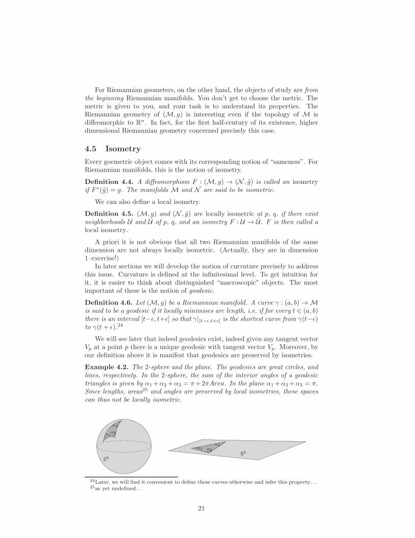
Example 4.2. The 2-sphere and the plane. The geodesics are great circles, andlines, respectively. In the 2-sphere, the sum of the interior angles of a geodesictriangles is given by α1+α2+α3 = π+2πArea. In the plane α1+α2+α3 = π.Since lengths, areas25 and angles are preserved by local isometries, these spacescan thus not be locally isometric.

S2

E2

α1

α3α2

α3

α1α2

24Later, we will find it convenient to define these curves otherwise and infer this property. . .25as yet undefined. . .

21

We will turn in the next section to the developing the tools necessary toconsider geodesics in Riemannian geometry. As we shall see, these are governedby ordinary differential equations. So we must first turn to the geometric theoryof such equations on manifolds.

5 Vector fields and O.D.E.’s

In this section we will develop the geometric theory of ordinary differentialequations, i.e. the theory of integral curves of vector fields on manifolds.

5.1 Existence of integral curves

Back to Rn. I will assume the following fact from the theory of ode’s26.

Theorem 5.1. Consider the initial value problem

(xi)′ = f i(x1, . . . xn), (8)

xi(0) = xi0, (9)

where f is a Lipschitz function in U ⊂ Rn. Then there exists a unique maximal(T−, T+), with −∞ ≤ T− < 0 < T+, and a unique continuously differentiablesolution

xi : (T−, T+)→ Rn

satisfying (8), (9). If f is smooth then x is smooth. Moreover, if T+ <∞, thengiven any compact subset K ⊂ U , there exists a tK such that x(tK , T+)∩K = ∅.

The geometric interpretation of this theorem is:

Theorem 5.2. Let V be a C∞ vector field on an open subset U ⊂ Rn. Thenthrough any point p in U , there exists a maximal parametrized integral curveγ of V , i.e. a curve γ : (T−, T+) such that γ′ = V , γ′(0) = p. Moreover, ifT+ < ∞, then given any compact subset K ⊂ U , there exists a tK such thatγ(tk, T+) ∩K = ∅.

The maxaimality statement is simply the following: If γ : (a, b) is anotherparametrized integral curve of V with γ(0) =, then T− ≤ a < b ≤ T+ andγ|(a,b) = γ.

In the example sheet you shall show that this can be extended to manifoldsas follows:

Theorem 5.3. Let M be a C∞ manifold, and let V be a C∞ vector field onM, i.e. V ∈ Γ(TM). Then through any point p in U , there exists a maximal27

parametrized integral curve γ of V , i.e. a curve γ : (T−, T+) such that γ′ = V ,γ′(0) = p.

p MVγ

26ode’s=ordinary differential equations27i.e. a curve not a subset of a larger such curve

22

Moreover, if T+ < ∞, then given any compact subset K ⊂ U , there exists atK such that γ(tK , T+) ∩K = ∅. In particular, if M itself is compact, then γ“exists for all t”, i.e. T± = ±∞.

Definition 5.1. If for all p, T± = ±∞, then we call X complete.

In this language, on a compact manifoldM, all vector fields X are complete.Exercise: Write down a manifold and an incomplete vector field. Write down

a non-compact manifold and a complete vector field. Does every non-compactmanifold admit an incomplete vector field?

5.2 Smooth dependence on initial data; 1-parameter groups

of transformations

Classical O.D.E. theory tells us more than Theorem 5.1. It tells us that solutionsdepend continuously (in the Lipschitz case) and smoothly (in the smooth case)on initial conditions.

To formulate this in the language of vector fields, let V ∈ Γ(TM).

Proposition 5.1. For every p ∈ M there exists an open set U , a nonemptyopen interval I and a collection of local transformations28

φt : U →M,

such that φt(q) is the integral curve of V through q given by Proposition 5.1.Moreover φ : U × I →M is a smooth map, and

φt ◦ φs = φt+s, (10)

on U ∩ φ−s(U), whenever t, s, t+ s ∈ I.

A family of local transformations satisfying (10) is called a 1-parameter localgroup of transformations. If I = R then φt are in fact “global” and (10) definesa group structure on {φt}.

Note that in particular, the above theorem says that |T±| can be uniformlybounded below in a neighborhood of any point.

It is easy to see using (10) that there is a one to one correspondence between1-parameter local groups of transformations and vector fields. Check the fol-lowing: Given such a family φt, define X(p) to be the tangent vector of φt(p) att = 0. The 1-parameter local group of transformations associated to X is againφt.

5.3 The Lie bracket

Let M be a smooth manifold, let X and Y be smooth vector fields: X,Y ∈Γ(TM).

Definition 5.2. [X,Y ] is the vector field defined by the derivation given by

[X,Y ]f = X(Y f)− Y (Xf).

28i.e. a smooth map U → M, where U ⊂ M, such that the map is a diffeomorphism to itsimage

23

Claim 5.1. For each p, [X,Y ]|p is indeed a derivation. [X,Y ] then defines asmooth vector field.

Proof. Check the properties of a derivation! Check smoothness!

Proposition 5.2. The following hold

1. [X,Y ] = −[X,Y ]

2. [X1 +X2, Y ] = [X1, Y ] + [X2, Y ]

3. [[X,Y ], Z] + [[Y, Z], X ] + [[Z,X ], Y ] (Jacobi identity)

4. [fX, gY ] = fg[X,Y ] + f(Xg)Y − g(Y f)XThe proof of this proposition is a straightforward application of the defini-

tion, left to the reader.So we can say that Γ(TM) is a (non-associative) algebra with the bracket

operation as multiplication. In general, algebras whose multiplication satisfies3 above are known as Lie algebras. Note finally, that if φ is a diffeomorphismthen

φ∗[X,Y ] = [φ∗X,φ∗Y ]. (11)

We say that φ∗ is a Lie algebra isomorphism.The above Proposition allows us to easily obtain a formula for [X,Y ] in

terms of local coordinates. If xi is a system of local coordinates, first note that[∂

∂xi,∂

∂xj

]= 0.

Now using in particular identity 4 of Proposition 5.2, setting X = X i ∂∂xi , Y =

Y i ∂∂xi , we have

[X,Y ] =

(X i ∂Y

j

∂xi− Y i ∂X

j

∂xi

)∂

∂xj.

Geometric interpretation of [X,Y ]. Let φt denote the one-parameter groupof transformations corresponding to X

Proposition 5.3.

[X,Y ]|p = limt→0

t−1(Y |p − ((φt)∗Y )p). (12)

Proof. Let ft denote f ◦ φt. Claim: ft = f + t(Xf) + t2ht where ht is smooth.Now, we clearly have

(φt)∗Y )pf = Yφ−1(p)(f ◦ φt).

Thus the right hand side of (12) applied to f is

lim t−1(Y |pf − Yφ−1(p)(f ◦ φt)) = lim t−1(Ypf − Yφ−1(p)(f + t(Xf) + t2ht))

= lim t−1(Ypf − Tφ−1(p)f)− Yp(Xf)= Xp(Y f)− Yp(Xf)= [X,Y ]p

as desired.

24

Proposition 5.4. Let φ be a diffeomorphism. If φt generates X, then φ−1◦φt◦φgenerates φ∗X. In particular, for φ and φt to commute, we must have φ∗X = X.

Proposition 5.5. [X,Y ] = 0 if and only if the 1-parameter local groups oftransformation commute.

Proof. Apply (12) to (φs)∗Y , use (11) and the relationship (φs)∗ ◦ (φt)∗ =(φs+t)∗.

5.4 Lie differentiation

The expression (12) looks like differentiation. It is and it motivates a moregeneral definition.

Letτ ∈ Γ∞(T ∗M⊗ · · · ⊗ T ∗M⊗ TM⊗ · · · ⊗ TM)

be a tensor field.Let φ :M→M be a diffeomorphism. We may define a tensor field φτ by

the formulaφτ()

Exercise. This indeed defines a smooth tensor field of the same type as τ .

Definition 5.3. Let X be a vector field and let φt denote the 1-parameter familyof local transformations generated by X. Let τ be a tensor field of general type.Then the Lie derivative of τ by X is defined to be

LXτ = limt=0

1

t(τ − φtτ).

We collect some properties here:

Proposition 5.6. We have

1. LXf = Xf

2. LXY = [X,Y ]

3. LX(τ1 + τ2) = LXτ1 + LXτ24. LX(τ1 ⊗ τ2) = LXτ1 ⊗ τ2 + τ1 ⊗ LXτ25. LfXgτ = fgLXτ + f(Xg)τ

6. LXC(τ) = C(LXτ).

6 Connections

With our toolbox from the theory of ode’s full, let us now return to the studyof geometry.

In this section we shall discuss the important notion of connection. Tomotivate this, let us begin from the study of geodesics in Rn, a.k.a. straightlines. The notion of connection is motivated by the classical interpretation ofthe geodesic equations in Rn that geodesics are characterised by the fact thattheir tangent vector does not change direction.

25

6.1 Geodesics and parallelism in Rn

We will begin with a discussion of the relevant concepts in the special case ofEuclidean space.

Let us call geodesics in Rn curves

γ : I → Rn

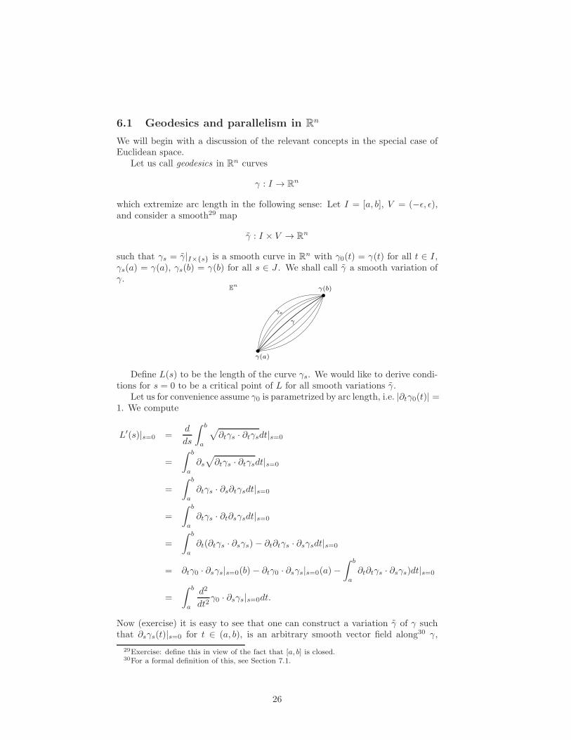
which extremize arc length in the following sense: Let I = [a, b], V = (−ǫ, ǫ),and consider a smooth29 map

γ : I × V → Rn

such that γs = γ|I×{s} is a smooth curve in Rn with γ0(t) = γ(t) for all t ∈ I,γs(a) = γ(a), γs(b) = γ(b) for all s ∈ J . We shall call γ a smooth variation ofγ.

En

γ(b)

γ(a)

γs

γ

Define L(s) to be the length of the curve γs. We would like to derive condi-tions for s = 0 to be a critical point of L for all smooth variations γ.

Let us for convenience assume γ0 is parametrized by arc length, i.e. |∂tγ0(t)| =1. We compute

L′(s)|s=0 =d

ds

∫ b

a

√∂tγs · ∂tγsdt|s=0

=

∫ b

a

∂s√∂tγs · ∂tγsdt|s=0

=

∫ b

a

∂tγs · ∂s∂tγsdt|s=0

=

∫ b

a

∂tγs · ∂t∂sγsdt|s=0

=

∫ b

a

∂t(∂tγs · ∂sγs)− ∂t∂tγs · ∂sγsdt|s=0

= ∂tγ0 · ∂sγs|s=0(b)− ∂tγ0 · ∂sγs|s=0(a)−∫ b

a

∂t∂tγs · ∂sγs)dt|s=0

=

∫ b

a

d2

dt2γ0 · ∂sγs|s=0dt.

Now (exercise) it is easy to see that one can construct a variation γ of γ suchthat ∂sγs(t)|s=0 for t ∈ (a, b), is an arbitrary smooth vector field along30 γ,

29Exercise: define this in view of the fact that [a, b] is closed.30For a formal definition of this, see Section 7.1.

26

vanishing at the endpoints. Thus, for the identity L′(0) = 0 to hold for allvariations γ,31 we must have

d2

dt2γ0 = 0. (13)

This is the geodesic equation in Rn. It is a second order ode. The generalsolution is

γ(t) = (x10 + a1t, . . . , xn0 + ant),

i.e. straight lines.We didn’t need any of the so-called qualitative theory of Section 5 to say

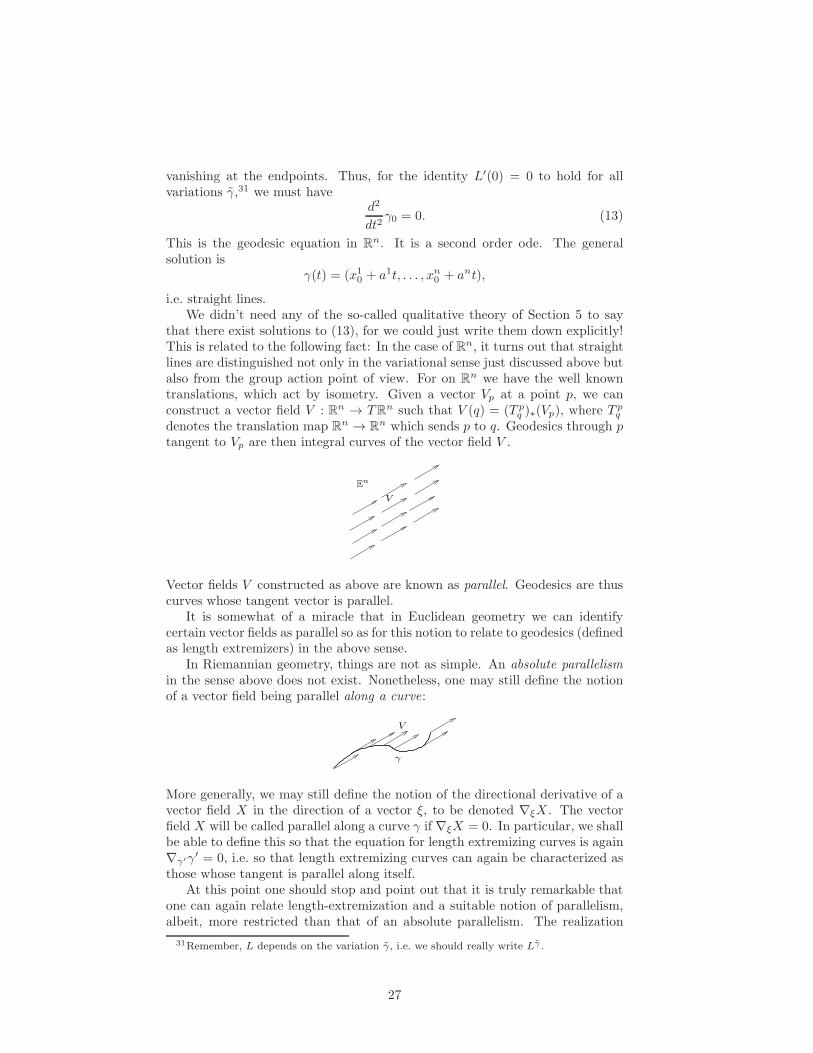
that there exist solutions to (13), for we could just write them down explicitly!This is related to the following fact: In the case of Rn, it turns out that straightlines are distinguished not only in the variational sense just discussed above butalso from the group action point of view. For on Rn we have the well knowntranslations, which act by isometry. Given a vector Vp at a point p, we canconstruct a vector field V : Rn → TRn such that V (q) = (T pq )∗(Vp), where T

pq

denotes the translation map Rn → Rn which sends p to q. Geodesics through ptangent to Vp are then integral curves of the vector field V .

V

En

Vector fields V constructed as above are known as parallel. Geodesics are thuscurves whose tangent vector is parallel.

It is somewhat of a miracle that in Euclidean geometry we can identifycertain vector fields as parallel so as for this notion to relate to geodesics (definedas length extremizers) in the above sense.

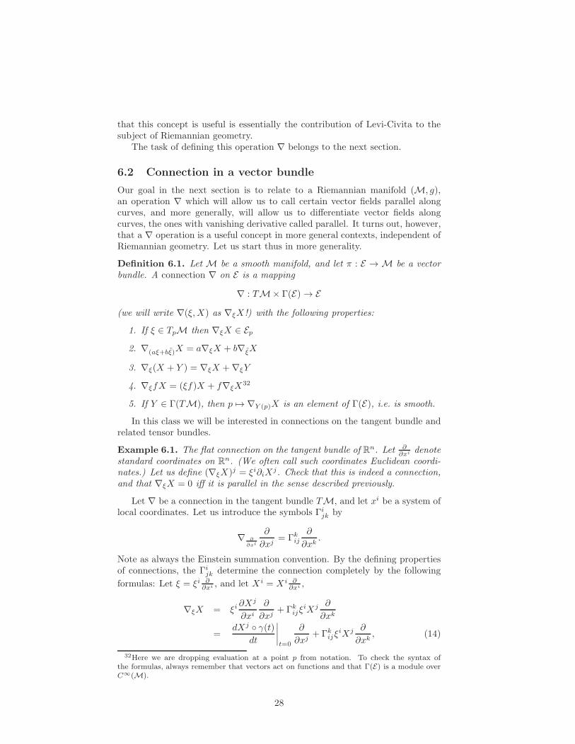
In Riemannian geometry, things are not as simple. An absolute parallelismin the sense above does not exist. Nonetheless, one may still define the notionof a vector field being parallel along a curve:

V

γ

More generally, we may still define the notion of the directional derivative of avector field X in the direction of a vector ξ, to be denoted ∇ξX . The vectorfield X will be called parallel along a curve γ if ∇ξX = 0. In particular, we shallbe able to define this so that the equation for length extremizing curves is again∇γ′γ′ = 0, i.e. so that length extremizing curves can again be characterized asthose whose tangent is parallel along itself.

At this point one should stop and point out that it is truly remarkable thatone can again relate length-extremization and a suitable notion of parallelism,albeit, more restricted than that of an absolute parallelism. The realization

31Remember, L depends on the variation γ, i.e. we should really write Lγ .

27

that this concept is useful is essentially the contribution of Levi-Civita to thesubject of Riemannian geometry.

The task of defining this operation ∇ belongs to the next section.

6.2 Connection in a vector bundle

Our goal in the next section is to relate to a Riemannian manifold (M, g),an operation ∇ which will allow us to call certain vector fields parallel alongcurves, and more generally, will allow us to differentiate vector fields alongcurves, the ones with vanishing derivative called parallel. It turns out, however,that a ∇ operation is a useful concept in more general contexts, independent ofRiemannian geometry. Let us start thus in more generality.

Definition 6.1. Let M be a smooth manifold, and let π : E → M be a vectorbundle. A connection ∇ on E is a mapping

∇ : TM× Γ(E)→ E

(we will write ∇(ξ,X) as ∇ξX!) with the following properties:

1. If ξ ∈ TpM then ∇ξX ∈ Ep2. ∇(aξ+bξ)X = a∇ξX + b∇ξX

3. ∇ξ(X + Y ) = ∇ξX +∇ξY

4. ∇ξfX = (ξf)X + f∇ξX32

5. If Y ∈ Γ(TM), then p 7→ ∇Y (p)X is an element of Γ(E), i.e. is smooth.

In this class we will be interested in connections on the tangent bundle andrelated tensor bundles.

Example 6.1. The flat connection on the tangent bundle of Rn. Let ∂∂xi denote

standard coordinates on Rn. (We often call such coordinates Euclidean coordi-nates.) Let us define (∇ξX)j = ξi∂iX

j. Check that this is indeed a connection,and that ∇ξX = 0 iff it is parallel in the sense described previously.

Let ∇ be a connection in the tangent bundle TM, and let xi be a system oflocal coordinates. Let us introduce the symbols Γijk by

∇ ∂

∂xi

∂

∂xj= Γkij

∂

∂xk.

Note as always the Einstein summation convention. By the defining propertiesof connections, the Γijk determine the connection completely by the following

formulas: Let ξ = ξi ∂∂xi , and let X i = X i ∂

∂xi ,

∇ξX = ξi∂Xj

∂xi∂

∂xj+ Γkijξ

iXj ∂

∂xk

=dXj ◦ γ(t)

dt

∣∣∣∣t=0

∂

∂xj+ Γkijξ

iXj ∂

∂xk, (14)

32Here we are dropping evaluation at a point p from notation. To check the syntax ofthe formulas, always remember that vectors act on functions and that Γ(E) is a module overC∞(M).

28

where γ(t) is any curve inM with γ′(0) = ξ.Clearly, connections can be constructed by prescribing arbitrarily the func-

tions Γkij and patching together with partitions of unity.

6.2.1 Γijk is not a tensor!

It cannot be stressed sufficiently that connections are not tensors. We shall see,for instance, that for all p ∈ M there always exists a coordinate system suchthat Γijk(p) = 0.

The transformation law for Γijk is given by

Γαβγ =∂xα

∂xµ∂2xµ

∂xβ∂xγ+ Γµνλ

∂xν

∂xβ∂xλ

∂xγ∂xα

∂xµ

The difference between two connections ∇− ∇, however is a tensor.

6.3 The Levi-Civita connection

Let us now return to Riemannian manifolds (M, g). It turns out that thereexists a distinguished connection ∇ that one can relate to g:

Proposition 6.1. Let (M, g) be Riemannian. There exists a unique connection∇ in TM characterized by the following two properties

1. If X, Y are vector fields then, ∇X(p)Y −∇Y (p)X = [X,Y ](p).

2. If X, Y are vector fields and ξ is a vector then ∇ξg(X,Y ) = g(∇ξX,Y )+g(X,∇ξY ).

Proof. Compute g(∇XY, Z) explicitly using the rules above, and show that thisgives a valid connection.

Since the Levi–Civita connection is determined by the metric one can easilyshow the following:

Proposition 6.2. Let (M, g), (M, g) be Riemannian and suppose that p ∈ U ⊂M, q ∈ U ⊂ M, and φ : U → V is an isometry with φ(p) = q. Let γ be a curvein U , and let V be a vector field along γ and let T be a vector tangent to γ. Let∇ and ∇ denote the Levi-Civita connections of M, M, respectively. Then

φ∗∇TV = ∇φ∗Tφ∗V .

In particular, if V is parallel along γ (i.e., ∇TV = 0), then φ∗V is parallelalong φ ◦ γ.

6.3.1 The Levi–Civita connection in local coordinates

The Levi-Civita connection in local coordinates. First some notation. We willdefine the inverse metric gij as the components of the bundle transformationT ∗M→ TM inverting the isomorphism TM→ T ∗M enduced by the Rieman-nian metric g. More pedestrianly, it is the inverse matrix of gij , i.e. we havegijgjk = δik where δik = 1 if i = k and 0 otherwise. Check that

Γkij =1

2gkl(∂jgil + ∂igjl − ∂lgij).

29

(Check also that the first condition in the definition of the connection is equiv-alent to the statement Γkij = Γkji.)

6.3.2 Aside: raising and lowering indices with the metric

Since we have just used the so-called inverse metric, we might as well discussthis topic now in more detail. This is the essense of the power of index notation.

The point is that given any tensor field, i.e. a section of

T ∗M⊗ · · · ⊗ T ∗M⊗ TM⊗ · · · ⊗ TM

we can apply the bundle isomorphism defined by the inverse metric on any ofthe T ∗M factors so as to convert it into a TM. And similarly, we can applythe isomorphism defined by the metric itself to turn any of the factors TM toconvert it to a T ∗M.

It is traditional in local coordinates to use the same letter for all the tensorsone obtains by applying these isomorphisms to a given tensor. I.e., if Sj1,...jmi1,...inis a tensor, then the tensor produced by applying the above isomorphism say tothe factor corresponding to the index ik is given in local coordinates by

Sj1...jnhi1...ik...in

= gikhSj1...jmi1...in.

The hat above denotes that the index is omitted.This process is known as raising and lowering indices.Thus, using the metric, we can convert a tensor to one with all indices up

or down, or however we like, and we think of these, as in some sense being the“same” tensor.

Finally, this process can be combined with the contraction map. For if saySijkl is a tensor, then we can raise the index i to obtain Sijkl, and now apply thecontraction map of Definition 3.8 on the factors corresponding to the indices iand j to obtain a tensor Skl. Again, one often uses the same letter to denotethis new tensor, as we have just done here, although there is a potential forconfusion, as one can define several different contractions, depending on theindices selected.

7 Geodesics and parallel transport

7.1 The definition of geodesic

We may now make the definition

Definition 7.1. Let (M, g) be a Riemannian manifold with Levi-Civita con-nection ∇. A curve γ : I →M is said to be a geodesic if

∇γ′γ′ = 0. (15)

Strictly speaking, equation (15) does not make sense, since γ′ is a vectorfield along γ, i.e. it can be though of as a section of the bundle γ∗(TN ) → I.Nonetheless, we can use formula (14) to define the left hand side of (15). Ingeneral, when V is a vector field along a curve γ, and W is a vector tangentto γ, we will use unapologetically the notation ∇WV . Similarly for vector

30

fields “along” higher dimensional submanifolds, defined in the obvious sense.(Exercise: What is this obvious sense?)

Note that in view of Proposition 6.2, local isometries map geodesics togeodesics. (Show it!)

It turns out that the above notion of geodesic coincides with that of curveslocally minimizing arc length:

Theorem 7.1. Let γ be a geodesic. Then for all p ∈ γ, there exists a neigh-borhood U of p, so that for all q, r ∈ γ ∩ U , denoting by γq,r the piece of γconnecting q and r, we have d(q, r) = L(γq,r), where L here denotes length, andmoreover, if γ is any other piecewise smooth curve in M connecting q and r,then L(γ) > d(q, r).

The proof of Theorem 7.1 is not immediate, and in fact, reveals various keyideas in the calculus of variations. We will complete the proof several sectionslater in these notes.

7.2 The first variation formula

For now let us give the following:

Proposition 7.1. A C2 curve γ : [a, b] → M is a geodesic parametrized bya multiple of arc length iff for all C2 variations γ : [a, b] × [−ǫ, ǫ] of γ withγ(a, s) = γ(a), γ(b, s) = γ(b), we have

d

dsL (γ(·, s))|s=0 = 0.

It is this Proposition that relates parellelism with length extremization,i.e. that allows us to recover the analogue in Riemannian geometry of the pictureof Section 6.1.

Proof. Let γ be a C2 curve, and let γ be an arbitrary variation of γ.Let us introduce the notation N = γ∗

∂∂s , T = γ∗

∂∂t , where s is a coordinate

in (−ǫ, ǫ) and t is a coordinate in [0, L]. And define L(s) to be the length of thecurve γ(·, s).

We have

L(s) =

∫ b

a

√g(Tγ(s,t), Tγ(s,t))dt.

We now have the technology to mimick the calculation in Section 6.1.

31

Differentiating L in s, we obtain

L′(s) =d

ds

∫ b

a

√g(T, T )dt

=

∫ b

a

N√g(T, T )dt

=

∫ b

a

(g(T, T ))−1/2g(∇NT, T )dt

=

∫ b

a

(g(T, T ))−1/2g(∇TN, T )dt

=

∫ b

a

T ((g(T, T ))−1/2g(N, T ))

− T (g(T, T ))−1/2)g(N, T )− (g(T, T ))−1/2g(N,∇TT )dt (16)

= g(T, T )1/2g(N, T )]ba

−∫ b

a

T (g(T, T ))−1/2g(N, T )− (g(T, T ))−1/2g(N,∇TT )dt (17)

=

∫ b

a

−T (g(T, T ))−1/2g(N, T )− (g(T, T ))−1/2g(N,∇TT )dt

=

∫ b

a

g(T, T )−3/2g(∇TT, T )g(N, T )− (g(T, T ))−1/2g(N,∇TT )dt.(18)

Here we have used [N, T ] = 0, ∇NT −∇TN = 0, and the fact that N(a, s) = 0,N(b, s) = 0. Exercise: Why are these statements true?

Now suppose that γ is a geodesic in the sense of Definition 7.1. Since∇TT |γ(0,t) = 0, the whole expression on the right hand side of (16) vanisheswhen evaluated at s = 0. Since γ is arbitrary, this proves one direction of theequivalence.

To prove the other direction, first we note that given any vector field N alongγ, there exists some variation γ such that N = γ∗

∂∂s . (A nice way to construct

such a vector field is via the exponential map discussed in later sections. But thisis not necessary.) Thus it suffices to show that if T does not satisfy ∇TT = 0,then there exists an N such that the expression on the right hand side of (16)is non-zero.

Suppose then that ∇TT (t0, 0) 6= 0. There exists a neighborhood (t1, t2) oft0 such that ∇TT (t, 0) 6= 0 for t ∈ (t1, t2). Let N be the vector field along γsuch that N(t) = ∇TT (t, 0). We have

∫ b

a

g(T, T )−3/2g(∇TT, T )g(N, T )− (g(T, T ))−1/2g(N,∇TT )dt

=

∫ b

a

g(T, T )−3/2g(∇TT, T )g(∇TT, T )− g(T, T ))−1/2g(∇TT,∇TT )dt

≤∫ t2

t1

g(T, T )−3/2g(∇TT, T )g(∇TT, T )− g(T, T ))−1/2g(∇TT,∇TT )dt

< 0.

The last inequality follows by noting that the above expression is −g(T, T )−1/2

32

times the norm squared of the projection of ∇TT to the orthogonal complementof T , and the latter is certainly nonnegative.

Thus, we must have ∇TT = 0.

7.3 Parallel transport

Our goal is to prove the existence of geodesics by reducing to the theory ofordinary differential equations. The geodesic equation in local coordinates is ofcourse a second order equation for γ. It is a first order equation for the tangentvector.

Let us first consider the following simpler situation. Let γ : I → M be afixed smooth curve, I = [a, b], denote γ(a) as p, γ(b) as q, and let T denote thetangent vector γ′. Suppose V is an arbitrary vector at p.

Proposition 7.2. There exists a unique smooth vector field V along γ suchthat V (a) = V and

∇T V = 0, (19)

i.e. so that V is parallel along γ.

Proof. Writing (19) for the components V x of V with respect to a local coordi-nate system, we obtain

d

dtV α = −ΓαβγT β(γ(t))V γ . (20)

Let us consider the manifold (−∞,∞)× Rn, and consider the vector field

(s, x) 7→ (s,−ΓαβγT β(γ(t))xβ),

where we set ΓαβγTβ(γ(s)) = ΓαβγT

β(γ(a)) for s < a, and ΓαβγTβ(γ(s)) =

ΓαβγTβ(γ(b)) for s > b. Then integral curves (s(t), V (t)) of this vector field

are precisely solutions of (20) for t values in [a, b], after dropping the s(t) whichclearly must satisfy s(t) = t.33 Thus, by Theorem 5.3, we have that for the ini-tial value problem at t = a, there exists a maximum future time T of existence,and a solution V (t) on [a, T ).

On the other hand, since the equation (20) is linear, we know a priori thata solution V is bounded by

∑

δ

|V δ(t− a)| ≤∑

δ

|V δ| exp((

supt,α,γ

ΓαβγTβ

)|t− a|

)

Thus, (s(t), V (t)) cannot leave every compact subset of (−∞,∞)×Rn in finitetime, and thus T =∞. In particular, V is defined in all of [a, b]

We call the vector W = V (q) the parallel transport of V to q along γ. Oneeasily sees that parallel transport defines an isometry Tγ : TpM → TqM oftangent spaces.

33We have just here performed a well known standard trick from ode’s for turning a so-callednon-autonomous system to an autonomous system.

33

7.4 Existence of geodesics

Now for the existence of geodesics:Since the geodesic equation is second order, to look for a first order equation,

we must go to the tangent bundle.34 Let xα be a system of local coordinates onM. Extend this to a system of local coordinates (x1, . . . xn, p1, . . . pn) on TM,where the pα are defined by

V =∑

pα(V )∂

∂xα

for any vector V .The geodesic equation (15), which in local coordinates can be written in

second order formd2xα

dt2= −Γαβγ

dxβ

dt

dxγ

dt,

can now be written asdxα

dt= pα (21)

dpα

dt= −Γαβγpβpγ . (22)

Solutions of the system (21)–(22) are just integral curves on TM of thevector field

pα∂

∂xα− Γαβγp

βpγ∂

∂pα

on TM. Remember, the latter is an element of Γ(T (TM)). Don’t be tooconfused by this. . .

We now apply Theorem 5.3, and Proposition 5.1. We call the one-parameterlocal group of transformations φt : TM → TM generated by this vector fieldgeodesic flow.

Projections π ◦ φt to M are then the geodesics we have been wanting toconstruct. We have thus shown in particular the following:

Proposition 7.3. Let Vp ∈ TM. Then there exists a unique maximal arc-length-parametrized geodesic γ : (T−, T+)→M such that γ′(0) = V0.

Thus, we have shown the existence of geodesics.

8 The exponential map

Back to φt. It is easy to see that the domain U of φt is star-shaped in the sensethat if Vp ∈ U , for some vector Vp at a point p, then λVp ∈ U for all 0 ≤ λ ≤ 1.Moreover, (exercise) φt(Vp) = φλ−1t(λVp). This implies, that φ1 is defined in anon-empty star-shaped open set.

Definition 8.1. The map exp : U →M defined by π ◦ φ1, where π denotes thestandard projection π : TM → M and U denotes the domain of φ1, is calledthe exponential map.

34Again, this is just a sophisticated version of the well known trick from ode’s of making asecond order equation first order.

34

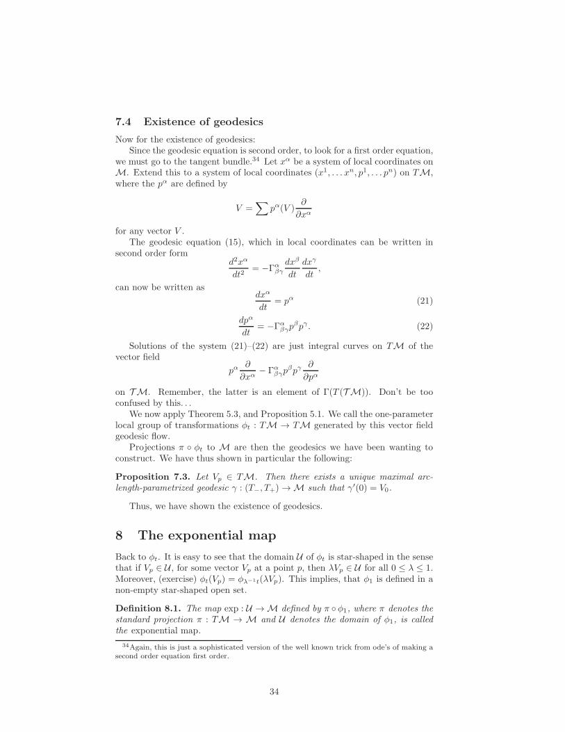
The map is depicted below:

γ

Vp

p

Mexp(Vp)

The curve γ(t) is a geodesic tangent to Vp, parametrized by arc length and

exp(Vp) = γ(|Vp|). Here |Vp| =√g(Vp, Vp).

As a composition of smooth maps, the exponential map is clearly a smoothmap of manifolds. In the next section, we shall compute its differential.

We end this section with a definition:

Definition 8.2. Let (M, g) be Riemannian. We say that (M, g) is geodesicallycomplete if the domain U of the exponential map is TM.

Equivalently, (M, g) is geodesically complete if all geodesics can be continuedto arbitrary positive and negative values of an arc length parameter.

8.1 The differential of exp

First a computation promised at the end of the last section. What is exp∗?First, what seems like a slightly simpler situation: for any p ∈ M let us

denote by expp the restriction of the map exp to Up = U ∩ TpM. This is alsoclearly a smooth map.

We will compute(expp∗

)0p. It turns out that this is basically a tautology.

The only difficulty is in the notation. Remember(expp∗

)0p

: T0p(TpM)→ TpM

On the other hand, in view of the obvious35

T0p(TpM) ∼= TpM, (23)

we can consider the map as a map:(expp∗

)0p

: TpM→ TpM.

Proposition 8.1. We have(expp∗

)0p

= id (24)

Proof. Let v ∈ TpM, and consider the curve t 7→ tv. Denote this curve in TpMby κ(t). This curve is tangent to v. The curve expp(κ(t)) is found by noting

expp(κ(t)) = expp(tv) = φt(v) = γ(|v|t) .= γ(t)

where φt denotes geodesic flow, and γ denotes the arc-length geodesic throughp tangent to v. By definition of the differential map, we have that

(exp∗)0p = γ′(t) = v,

thus, we have obtained (24).

35define it!

35

A little more work (equally tautological as the above) show that

(π × exp∗)0p : TpM× TpM→ TpM× TpM is invertible (25)

as it can be represented as a block matrix consisting of the identity on thediagonal. Here it is understood that

π × exp : TM→M×M

π× exp(vp) = (p, exp(vp)). Again, the domain and range of the differential maphave been identified with TpM× TpM by obvious identifications analogous to(23) that the reader is here meant to fill in.

What is the point of all this? We can now apply the following inverse functiontheorem

Theorem 8.1. Let F : M → N be a smooth map such that (F∗)p : TpM →TqN is invertible. Then there exists a neighborhood U of p, such that F |U is adiffeomorphism onto its image.

Proof. Prove this from the inverse function theorem on Rn.

Applied to the map π × exp, in view of this gives the following:

Proposition 8.2. Let p ∈ (M, g). There exists a neighbhorhood U = U × Uof (p, p) inM×M such that, denoting by W = (π × exp)−1(W), we have thatπ × exp |W :W → U × U is invertible.

That is to say, for any points q1, q2 ∈ U , there exists a vq1 ∈ Tq1M such thatexp(vq1) = q2. (Exercise in tautology: why does this statement follow from theproposition?)

A moment’s thought tells us that we can slightly refine the above Proposi-tion. Let us choose ǫ > 0 so that

B0q (ǫ) ∩W = ∪q ∈ UB0q (ǫ).= W .

Again, π×exp |W is a diffeomorphism, and its projection to the first componentis U . Let V ⊂ U such that V × V is in the image of this. Let q1, q2 ∈ V . Thenthere exists a vq1 ∈ Tq1M such that exp(vq1) = q2, and moreover, such that|vq1 | < ǫ.

Note that the curve t→ exp(tvq1), 0 ≤ t ≤ 1 is contained completely in W .We have thus produced a neighborhood V with the property that there exists

an ǫ > 0 such that any two points q1 and q2 of V can be joined by a geodesic γof length < ǫ. Moreover, any other geodesic joining q1 and q2 must have length≥ ǫ. Why?

We can in fact refine this further: We shall prove that γ has length < anycurve joining q1 and q2. Moreover, we shall show that V can be chosen so thatγ is completely contained in V . Such a neighbhorhood is called a geodesicallyconvex neighborhood.

8.2 The Gauss lemma

For this, we need a computation originally done in the setting of surfaces in R3

by Gauss.

36

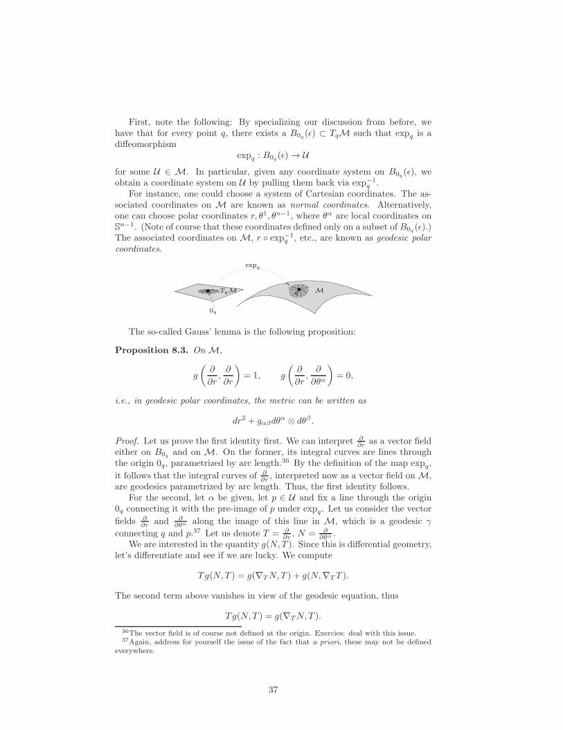
First, note the following: By specializing our discussion from before, wehave that for every point q, there exists a B0q (ǫ) ⊂ TqM such that expq is adiffeomorphism

expq : B0q (ǫ)→ Ufor some U ∈ M. In particular, given any coordinate system on B0q (ǫ), weobtain a coordinate system on U by pulling them back via exp−1

q .For instance, one could choose a system of Cartesian coordinates. The as-

sociated coordinates on M are known as normal coordinates. Alternatively,one can choose polar coordinates r, θ1, θn−1, where θα are local coordinates onSn−1. (Note of course that these coordinates defined only on a subset of B0q (ǫ).)The associated coordinates onM, r ◦ exp−1

q , etc., are known as geodesic polarcoordinates.

MqTqM

0q

expq

The so-called Gauss’ lemma is the following proposition:

Proposition 8.3. OnM,

g

(∂

∂r,∂

∂r

)= 1, g

(∂

∂r,∂

∂θα

)= 0,

i.e., in geodesic polar coordinates, the metric can be written as

dr2 + gαβdθα ⊗ dθβ .

Proof. Let us prove the first identity first. We can interpret ∂∂r as a vector field

either on B0q and on M. On the former, its integral curves are lines throughthe origin 0q, parametrized by arc length.36 By the definition of the map expq,

it follows that the integral curves of ∂∂r , interpreted now as a vector field onM,

are geodesics parametrized by arc length. Thus, the first identity follows.For the second, let α be given, let p ∈ U and fix a line through the origin

0q connecting it with the pre-image of p under expq. Let us consider the vector

fields ∂∂r and ∂

∂θα along the image of this line in M, which is a geodesic γ

connecting q and p.37 Let us denote T = ∂∂r , N = ∂

∂θα .We are interested in the quantity g(N, T ). Since this is differential geometry,

let’s differentiate and see if we are lucky. We compute

Tg(N, T ) = g(∇TN, T ) + g(N,∇TT ).

The second term above vanishes in view of the geodesic equation, thus

Tg(N, T ) = g(∇TN, T ).36The vector field is of course not defined at the origin. Exercies: deal with this issue.37Again, address for yourself the issue of the fact that a priori, these may not be defined

everywhere.

37

On the other hand, since [N, T ] = 0, we have

Tg(N, T ) = g(∇TN, T ) = g(∇NT, T ) =1

2Ng(T, T ) = 0

since g(T, T ) = 1 identically. Thus g(N, T ) is constant along γ. Since N = 0 atq, then g(N, T ) = 0 identically.

The above lemma leads immediately to the following

Proposition 8.4. Let q, ǫ, U be as in the above lemma, and let p ∈ U . Thenthe radial geodesic γ joining q and p, of length r(p), is length minimizing, i.e. ifγ is any other piecewise regular curve joining q and p, then L(γ) > L(γ) = r(p).

The statement is in fact true where piecewise regular is replaced by anyrectifiable curve. These are the most general curves for which one can definethe notion of length.

Proof. For a piecewise regular curve, we can write the length as

L =

∫ √g(γ′, γ′)dt.

Let us consider separately the case where γ ⊂ U , and when it is not. In theformer case, since the curve is contained in our geodesic polar coordinate chart38,we can write

L =

∫ √(dr

dt

)2

+ gαβdθα

dt

dθβ

dtdt (26)

≥∫ √(

dr

dt

)2

dt

≥∫dr

dtdt

= r(p),

with equality iff39 gαβdθα

dtdθβ

dt = 0, and thus θα = c, and drdt 6= 0. Thus, after

reparametrization, γ is the radial geodesic.In the other case, there is a first time t0 when γ crosses r = r(p). Redo the

above with γ replaced by γ|[0,t0].

The above argument actually illustrates a general technique in the calculusof variations for showing that the solution of a variational problem is actuallya minimiser. The technique is called: embedding in a field of variations.

8.3 Geodesically convex neighbourhoods

We can now turn to finishing up a task left undone, namely showing the existenceof geodesically convex neighbourhoods in the sense described previously.

First a remark. There is something we can say about non-radial geodesicscompletely contained in a geodesic polar coordinate chart. If κ is such a geodesic

38Again, with the usual caveat.39Exercise: Why is this expression positive definite?

38

then r ◦ κ cannot have a strict maximum. For suppose tmax were such a point.

Note that a tmax,d2rdt2 ≤ 0, drdt = 0. But,

d2r

dt2(tmax) = −Γrβγ

dθβ

dt

dθγ

dt

= −1

2grr(−∂rgβγ)

dθβ

dt

dθγ

dt

=1

2∂rgβγ

dθβ

dt

dθγ

dt> 0

Exercise: why the last strict inequality? This is a contradiction.We can finally complete our construction of a geodesically convex neigh-

borhood. Let W be as in Proposition 8.2. We may choose ǫ as in the dis-cussion after that Proposition, and and choose a V as before, but with ǫ/2 inplace of ǫ, and so that addition V is of the form expp(B0p(ǫ/4). We have thatV ⊂ expp(B0p(ǫ)) ⊂ W . Moreover, we have that any two points q1, q2 in V can

be joined by a geodesic in W of length < 12ǫ.

Repeating a previous computation (namely, (26), it follows that such ageodesic necessarily must remain in expp(B0p(ǫ)). Thus, by our result on theabsense of maxima of r, it follows that r cannot have a maximum. Sincer(q1) < ǫ/4, r(q2) < ǫ/4, it follows that r < ǫ/4 throughout the geodesic.That is to say, the geodesic is contained in V . So V is geodesically convex inthe sense claimed.

8.4 Application: length minimizing curves are geodesics

In later sections, we shall give conditions on a Riemannian manifold implyingthe existence of length minimizing geodesics joining any two given points. Theconstruction of these will involve global considerations.

On the other hand, given a curve which is not a geodesic, one can show thatit can not be length minimizing by completely local considerations. This is infact yet another application of what we have just done.

Proposition 8.5. Let (M, g) be Riemannian, with p, q ∈ M, and let γ be apiecewise regular curve from p to q. If γ is not a geodesic, then there exists apiecewise regular curve γ connecting p to q, such that L(γ) < L(γ).

Proof. Suppose γ is not a geodesic. Then there exists a point p = γ(T ) whereγ does not satisfy the geodesic equation. Consider a geodesically convex neigh-borhood V centered at p. Consider two points q1, q2 on γ, in V , such that sayγ(t1) = q1, γ(t2) = q2, with t1 < T < t2. We know that there exists a geodesicconnecting q1 and q2 which is length minimizing. If this geodesic coincides withγ|[t1,t2], then there is nothing to show. If not, then the curve γ|[t1,t2] has strictlygreater length than this curve, in which case we can replace γ by a shorter curvejoining p and q.

39

9 Geodesic completeness and the Hopf-Rinow

theorem

9.1 The metric space structure

An application of the previous is to show that a Riemannian manifold inheritsthe structure of a metric space related to the Riemannian metric.

Definition 9.1. Let (M, g) be a Riemannian manifold. For x, y ∈M, let Gx,ydenote the set of all piecewise smooth curves joining x and y, and for γ ∈ Gx,y,let L(γ) denote the length of the curve γ¿ Define

d(x, y) = infγ∈Gx,y

L(γ)

We have

Proposition 9.1. The function d defines a distance function onM, i.e. (M, d)is a metric space.

Proof. That d(x, y) = d(y, x) is obvious. The triangle inequality is similarlyimmediate. To spell it out: If γ : [a, b]→M is a piecewise smooth curve joiningx and y, and γ : [a, b] is a piecewise curve joining y and z, then γ : [a, b+ b− a]→M defined by γ(t) = γ(t) for t ∈ [a, b], γ(t) = γ(t) for t ∈ (b, b + b − a] is apiecewise smooth curve joining x and x with L(γ) = L(γ) + L(γ). Takinginfimums over Gx,y, Gy,z, one obtains the triangle inequality d(x, z) ≤ d(x, y)+d(y, z).

That d(x, x) ≥ 0 is obvious. If x 6= y, then let U be a geodesically convexneighborhood of x not containing y. In particular, U contains a geodesic sphereof radius ǫ. Any curve γ joining x and y must cross this geodesic sphere at somepoint p. Since the radial geodesic from x to p minimizes the length of all curvesfrom x to p, and the length of this curve is ǫ, it follows that L(γ) > ǫ. Thusd(x, y) ≥ ǫ.

9.2 Hopf–Rinow theorem

Recall from Section 7.4 the definition of geodesic completeness. In view of themetric space structure, we now have a “competing” notion of completeness,namely, metric completeness. In this section we shall show that this notion isactually equivalent to the notion of geodesic completeness defined earlier. In theprocess, we shall show that in a geodesically complete Riemannian manifold, itfollows that any two points can be connected by a (not necessarily unique!)length-minimizing geodesic. This result is essential for global arguments inRiemannian geometry. We shall get a taste of this in the final section.

Theorem 9.1. Let (M, g) be a Riemannian manifold, let x, y ∈ M, and sup-pose expx is defined on all of TxM. Then there exists a geodesic γ : [0, L]→Msuch that

L(γ) = d(x, y). (27)

Clearly, the assumptions of the above theorem are satisfied if (M, g) isgeodesically complete. Note that in view of the fact that L(γ) ≥ d(x, y), (27)is equivalent to the statement that for any other curve γ joining x and y, thenL(γ) ≥ L(γ).

40

Proof. Let Ux be a geodesically convex neighborhood of x, and let Sǫ be ageodesic sphere around x of radius ǫ > 0, contained in Ux, such that ǫ <d(x, y) = d. Since d(·, y) is a continuous function on Sǫ, and Sǫ is compact, itfollows that there exists a p ∈ Sǫ such that d(p, y) = infq∈Sǫ d(q, y). Considernow the radial geodesic γ from x through p, parametrized by arc length. Byassumption, γ(t) is defined for all values of t. We will show that γ(d) = y. Thiswill give the result of the theorem.

Note that γ(ǫ) = p. Consider the subset X ⊂ [ǫ, d] defined by

X = {s ∈ [ǫ, d] : d(y, γ(s′)) = d− s′, ∀ǫ ≤ s′ ≤ s}.

Clearly, our result follows if we show d ∈ X . Moreover,X is non-empty, because,we have ǫ ∈ X . To see this note first that every curve κ joining x and y mustcross Sǫ, points in the connected component ofM\Sǫ containing p have distance< ǫ away from x. Thus the length of κ is greater than ǫ plus the length of acurve from Sǫ to y. Thus d(x, y) ≥ d(p, y) + ǫ. On the other hand the reverseinequality is immediate from the triangle inequality. So indeed ǫ ∈ X .

Thus, since [ǫ, d] is connected, it suffices to show that X is open and closedin the topology of [ǫ, d].

The closedness of X is immediate in view of the continuity of the functiond(y, ·). To show that X is open, it suffices to show that if s ∈ X with s < d,then s+ δ ∈ X for δ sufficiently small.

So let s ∈ X , s < d. There exists a geodesically convex neighborhood U ofγ(s). Let δ be such that the geodesic sphere around γ(s) of radius δ, denotedSδ, is contained in U , and so that, moreover, δ < s < s + δ < d. (This will betrue for all δ ≤ δ0 for some δ0 > 0.) As before, let p minimize the distance fromSδ to y. Defining γ to be the radial geodesic from γ(s) to p, it follows as beforethat d(p, y) = d(γ(s), y) + δ.

Consider now the distance between γ(s − δ) and p. On the one hand, wehave, since s − δ ∈ X , that d(y, γ(s − δ)) = d − s + δ. On the other hand, weknow that

d(y, γ(s− δ)) ≤ d(γ(s− δ), p) + d(p, y) = d(γ(s− δ), p) + d− s− δ.

Thusd(γ(s− δ), p) ≥ 2δ.

On the other hand, by the triangle inequality, we have

d(γ(s− δ), p) ≤ 2δ.

Thus we have d(γ(s − δ), p) = 2δ. But since γ followed by γ is a curve joiningγ(s− δ) and p of precisely length 2δ, it follows by the properties of geodesicallyconvex neighborhoods that this curve is a geodesic, i.e. γ must coincide with γ.But now the claim follows, since p = γ(s+ δ).

Theorem 9.2. Let (M, g) be a Riemannian manifold, and suppose there existsa point x satisfying the assumptions of the previous Theorem. Then (M, d) iscomplete as a metric space.

In particular, the theorem applies in the case (M, g) is assumed geodesicallycomplete.

41

Proof. A metric space is complete if every Cauchy sequence converges. Compactspaces are complete, and Cauchy sequences are clearly bounded. Thus it sufficesto show that all bounded subsets of S are contained in compact sets.

Let B ⊂ M be bounded. This means that there exists an ∞ > M > 0such that d(x, y) ≤ M for all y ∈ M. By Theorem 9.1, this implies thatB ⊂ expx(BM (0)) wheere BM (0) denotes the closed ball of radius M in theTxM. But expx : TxM→M is a continuous function and BM (0) is compact.Thus expx(BM (0)) is compact and our theorem follows.

Theorem 9.3. Let (M, g) be a Riemannian manifold, and suppose (M, d) ismetrically complete. Then (M, g) is geodesically complete.

Proof. Let γ : [0, T ) → M be a geodesic parametrized by arc length, withT <∞. We shall show that γ can be extended to a geodesic γ : [0, T +δ)→M.

Let ti → T . Since d(γ(ti), γ(tj)) ≤ |ti − tj|, it follows that γ(ti) is Cauchy.By assumption then, γ(ti) converges to a point y. Let U denote a geodesicallyconvex neighborhood of y, and let ǫ be such that for every x1, x2 ∈ U , thereexists a unique geodesic γ of length ǫ inM starting from x1, with the propertythat x2 is on this geodesic within length ǫ. Choose γ(ti), γ(ti+1) ∈ U , withT − ti < ǫ, and consider the geodesic γ joining γ(ti) and (γ(ti+1) describedabove. Since γ is also a geodesic joining γ(ti) and γ(ti+1) of length less than ǫ,it follows that γ(t− ti) must coincide with γ(t) for t ∈ [ti, T ). Define now γ(t)for t ∈ [T, ti + ǫ) by γ(t) = γ(t− ti). This is then the required extension.

10 The second variation

The existence of length minimizing geodesics rests on a global argument. On theother hand, a length minimizing geodesic certainly must be length minimizingto local deformations. The condition that a geodesic be length minimizing tolocal deformations is characterized by a differential condition, analogous to thecharacterization f ′′ ≤ 0 for local minima of a function of one variable. It is in thischaracterization that the so-called curvature tensor first makes its appearance.

Let γ : [0, L]×(−ǫ, ǫ)→M denote a variation of a smooth curve γ : [0, L]→M, i.e., let γ be a smooth map such that γ(·, 0) = γ, and such that γ(·, s) isa curve for all s ∈ (−ǫ, ǫ). We have already computed a formula for the firstvariation in Section 7.1. We now go further and compute a formula for thesecond variation.

We shall compute this formula in the special case that the original γ is ageodesic parametrized by arc length (so then L is its length), and such that

γ(0, s) = γ(0, s), γ(L, s) = γ(L, s). (28)

It is a good exercise for the reader to write down the general case!Let us recall the notation N = γ∗

∂∂s , T = γ∗

∂∂t , where s is a coordinate

in (−ǫ, ǫ) and t is a coordinate in [0, L]. Also recall the notation L(s) got thelength of the curve γ(·, s).

We have (as in Section 7.2) that for all s.

L′(s) =

∫ L

0

(g(T, T ))−1/2g(T,∇NT )dt

42

Differentiating in s, and evaluating at 0, we obtain (using that g(Tγ(t,0), Tγ(t,0)) =1

L′′(0) =d

ds

∫ L

0

(g(T, T ))−1/2g(T,∇NT )dt|s=0

=

∫ L

0

−g(T, T )−3/2(g(T,∇NT ))2 + (g(T, T ))−1/2Ng(T,∇NT )dt|s=0

=

∫ L

0

g((∇NT,∇NT )− (g(T,∇NT ))2 + g(T,∇N∇NT )dt

=

∫ L

0

g(Π∇NT,Π∇NT ) + g(T,∇N∇NT )dt

=

∫ L

0

g(Π∇TN,Π∇TN) + g(T,∇N∇TN)dt

where Π denotes the projection to the orthogonal complement of the span ofT . We have used in the last line the relation [N, T ] = 0 and the torsion freeproperty of the connection.

At this point, let us momentarily specialize to the case of Rn with its Eu-clidean metric. In this case, covariant derivatives commute. (Why?) Wemay thus write

L′′(0) =

∫ L

0

g(Π∇TN,Π∇TN) + g(T,∇N∇TN)dt

=

∫ L

0

g(Π∇TN,Π∇TN) + g(T,∇T∇NN)dt

=

∫ L

0

g(Π∇TN,Π∇TN)dt− g(T,∇NN)]L0 +

∫ L

0

g(∇TT,∇NN)dt

=

∫ L

0

g(Π∇TN,Π∇TN)dt

where we have used ∇TT |γ(t,0) = 0 and the boundary condition (28) implyingN(γ(0)) = N(γ(L)) = 0.

In particular, we see that in this case L′′(0) ≥ 0, and thus geodesics min-imise40 arc length with respect to near-by variations.

Of course, in the case of Euclidean space, we already knew much more,namely that geodesics globally minimize arc length, i.e. that a geodesic fromp to q has the property that its length is strictly less than the length of anyother curve from p to q. (In particular, geodesics are unique.) This follows fromwhat we have done already, in view of the existence (for Rn) of global geodesicnormal coordinates, and Gauss’s lemma.

But no matter. It is merely this computation for L′′ that we wish to gen-eralize to Riemannian manifolds. Now, however, covariant derivatives no

longer commute. The analogue of the previous is given as below:

L′′(0) =

∫ L

0

g(Π∇TN,Π∇TN) + g(∇N∇TN −∇T∇NN, T )dt

=

∫ L

0

g(∇TN,∇TN) + g(R(T,N)N, T )dt (29)

40Show that L′′(0) > 0 for all non-trivial variations satisfying (28).

43

whereR(T,N)N = ∇N∇TN −∇T∇NN. (30)

The expression R(T,N)N is called the curvature. A priori it seems that itsvalue at a point p should depend on the behaviour of the vector fields T and Nup to second order. (If this were the case, then the formula (29) would not beparticularly useful.) But it fact, R(T,N)T depends only on T (p), N(p), i.e. Ris a a tensor. (See the next section!) As we shall see, R is an invariant ofthe metric g; it is the above expression for L′′ which gives it perhaps its mostnatural geometric interpretation in terms of the lengths of nearby curves.

We commence in the following section a systematic discussion of the cur-vature tensor. We will then return to the second variation formula, and use itto prove theorems relating local assumptions on the behaviour of the curvaturetensor, and global geometric properties of the manifold.

11 The curvature tensor

Having got a taste of curvature we now make the general definitions.

Definition 11.1. Let (M, g) be a Riemannian manifold, p ∈ M, and X, Y ,and Z be vetor fields in a neighborhood of p. We define

R(X,Y )Z = ∇Y∇XZ −∇X∇Y Z −∇[Y,X]Z

Proposition 11.1. R(X,Y )Z only depends on X(p), Y (p), and Z(p), i.e. Rcan be thought of as a section of TM⊗ T ∗M⊗ T ∗M⊗ T ∗M.

Proof. As usual, an uninspired calculation.

We call R the Riemann curvature tensor. The curvature tensor satisfies thefollowing symmetries

Proposition 11.2.

R(X,Y )Z = −R(Y,X)Z

g(R(X,Y )Z,W ) = −g(R(X,Y )W,Z)g(R(X,Y )Z,W ) = g(R(Z,W )X,Y )

R(X,Y )Z +R(Z,X)Y +R(Y, Z)X = 0

Proof. Again, this is just a computation. The last identiy is known as the firstBianchi identity.

Note why the Lie bracket term was absent in (30).

11.1 Ricci and scalar curvature

The algebraic complexity of curvature, and the more subtle relations of thiscomplexity and geometry, is something which we will not in fact really cometo terms with in this class. Here, we shall consider algebraically more simpleobjects that can be obtained from the Riemann curvature.

44

We can define the so called Ricci curvature by applying the contraction C ofDefinition 3.8. Specifically, considering R as a section of TM⊗T ∗M⊗T ∗M⊗TM, we may apply the map

C : TM⊗ T ∗M⊗ T ∗M⊗ T ∗M→ T ∗M⊗ T ∗M

acting as in Definition 3.8 but only in TM and the second T ∗M factor, i.e theone “corresponding” to Y in the notation R(X,Y )Z. The composition of C andR produces a tensor Ric which is a section of T ∗M⊗T ∗M. This is the so-calledRicci curvature. Alternatively, in view of the relation between contraction andtrace of a homomorphism, one easily sees that

Ric(X,Z) = traceY 7→ R(X,Y )Z.

From the symmetries of curvature tensor one sees that this is the only non-trivial contraction. Moreover, one sees that the Ricci tensor is symmetric,i.e. that Ric(X,Y ) = Ric(Y,X).

It is hard to give a sense at this stage for why the Ricci curvature is soimportant an object in geometry. Written in local coordinates (see next section)it has the same number of components as the metric, and this very pedestrianreason may be why it was first written down. But its true geometric characteris much more subtle. In this class, we will only scratch the surface, but we shallsee it used in Theorem 12.1 of Section 12.

In general relativity, the importance of Ricci curvature is clear from thebeginning. The vacuum Einstein equations are the statement that

Ric = 0

A further contraction of Ric (after raising one of the indices!) yields theso-called scalar curvature. This is often denoted by R, in the spirit of remarksgiven in Section 6.3.2. For a formula in terms of indices, see Section 11.3.

11.2 Sectional curvature

The reader familiar with the classical differential geometry of surfaces will havesome intuition for the Gauss curvature of a surface, in particular, what it meansgeometrically for the Gauss curvature to be positive, negative, zero.

It turns out that the curvature tensor defines, for each 2-plane, a notion ofcurvature that can be thought to correspond to the Gauss curvature. This iscalled the sectional curvature. It is defined as follows. Given a plane

Π ⊂ TpM

choose vectors X , Y spanning Tp. Define

K(Π) =g(R(X,Y )X,Y )

g(X,X)g(Y, Y )− g(X,Y )2.

Note that if X and Y are orthonormal, then

K(Π) = g(R(X,Y )X,Y )

45

Note that if M is two dimensional, then K coincides with the usual Gaussiancurvature.

It turns out that the condition K(Π) > 0 for all Π is most like the conditionof positive Gaussian curvature for surfaces. Similarly, K(Π) < 0. The subtletyof higher dimensional geometry lies in that K(Π) can have different signs fordifferent planes. The condition that Ric is positive (resp. negative) definite canbe thought of as a weaker analogue of K(Π) > 0 for all Π, (resp. K(Π) < 0 forall Π). We shall get at least some taste of all this in Section 12.

Finally, as an exercise, test your multilinear algebra skills by showing that thecollection of all sectional curvatures determines the Riemann curvature tensor.

11.3 Curvature in local coordinates

Since as we saw in the previous section, R can be though of as a section ofTM⊗ T ∗M⊗ T ∗M⊗ T ∗M, we can write it as

R = Rijkl∂

∂xi⊗ dxj ⊗ dxk ⊗ dxl

where

Rijkl∂

∂xi= R

(∂

∂xk,∂

∂xl

)∂

∂xj

Note: There is never universal agreement in the literature as to the order of theindices, or even the sign convention in the definition of the Riemann curvaturetensor. Sectional and Ricci curvature are always defined so as to be positive on,say Sn.

One can derive from the definition of curvature the formulas

Rijkl =∂Γijk∂xl

−∂Γijl∂xk

+ ΓmjkΓiml − ΓmjlΓ

imk

Ricij = Rkijk

R = gijRij .

Thus, if one has explicit formulas for the metric, one can compute the cur-vature tensor by brute force.

11.4 Curvature as a local isometry invariant

In view of Proposition 6.2, we have immediately that

Proposition 11.3. Let (M, g), (M, g) be Riemannian and suppose that p ∈U ⊂ M, q ∈ U ⊂ M, and φ : U → V is an isometry with φ(p) = q. Let R, Rdenote the Riemann curvature tensors of M, M respectively. Then

R(φ∗X,φ∗Y )φ∗Z = φ∗(R(X,Y )Z).

This is the statement that curvature is a local isometry invariant.An alternative (and quite cumbersome) way of proving Proposition 11.3 is

via the interpretation of curvature in terms of the second variation of arc length.Try it for yourself if you’re of that persuasion.

46

11.5 Spaces of constant curvature

11.5.1 Rn

It should be clear from the definition that in this case we have

Rlijk = 0.

In fact, the following statement is true. Let U be homoeomorphic to the n-disc,and let g be a metric on U such that Rlijk . Then there exists a smooth mapφ : U → Rn which is an isometry onto its image. In other words, if (M, g)has identically vanishing Riemann curvature, then M is locally isometric toEuclidean space.

The above statement was in fact proven by Riemann in his original lecturewhich initiated Riemannian geometry. In view also of Propostion 11.3, we seethat Rlijk = 0 are necessary and sufficient conditions for a Riemannian manifoldto be locally isometric to Euclidean space. This was the original motivation foridentifying this expression.

11.5.2 Sn

Write down the metric of Sn explicitly, and compute the curvature. In particu-lar, show that

K(Π) = 1

for all planes Π ⊂ TSn. We say that Sn is a space of constant curvature.Exercise: How can you cheat in this computation?Note that, in particular, the curvature tensor is not identically 0. In view

of Proposition 11.3, this gives a purely infinitessimal proof that the sphere andEuclidean space are not locally isometric. (Compare with Example 4.6, wherethe “macroscopic” formula for the area of spherical triangles is used. Actually,this formula can be derived by integrating the curvature in the spherical triangle.This is the celebrated Gauss-Bonnet formula.)

11.5.3 Hn

This space, called hyperbolic n-space, is the higher dimensional analogue of thespace H2 discussed in the introduction.

A useful way of representing this space is as the standard open disc in Rn

with metric

g =4

(1− (x1)2 − · · · − (xn)2)2e

where e denotes the standard Euclidean metric.Compute for yourself the curvature. In particular, show

K(Π) = −1

for all Π.It turns out that Riemannian manifolds of constant curvature are locally

isometric to Hn, Sn or Rn. This is not so difficult to show, but we will not showit here. . .

There is no end to the study of Sn, Hn, and their various quotients. A goodgeometer should be able to navigate these with ease.

47

12 Simple comparison theorems

12.1 Bonnet–Myers theorem

Theorem 12.1. (Bonnet-Myers) Let (M, g) be a complete Riemannian mani-fold with

Ric(X,X) ≥ (n− 1)kg(X,X)

for all X ∈ TM, for some k > 0. Then the diameter ofM is less than or equalto π/

√k . In particular, M is compact.

This is a protypical result of its kind in Riemannian geometry. A weak globalassumption (completeness), together with a curvature assumption, give a stronggeometric statement (diameter bounded) and more information on the topology(compactness).41

Note that the diameter is defined as supx,y∈M d(x, y).

Proof. Let x, y ∈ M. By Theorem 9.1, there exists a geodesic γ : [0, d] → M,parametrized by arc length, with γ(0) = x, γ(d) = y, and L(γ) = d = d(x, y).It suffices to show that d ≤ π/

√k.

Since γ is length minimizing, then if γ is any variation with fixed endpoints,we must have, for the corresponding function L(s), L′′(s) ≥ 0.

Now given a vector field along γ, vanishing at t = 0 and t = d, we can definea variation γ as above. We will define our vector fields (and thus our variations)by making use of an important technique in differential geometry, namely, thechoice of a well adapted frame, i.e. a well adapted set of orthogonal vectorsspanning the tangent at each point along γ.

In our case, a convenient such frame can be constructed as follows. LetE1, . . . En−1, denote vectors at γ(0) such that the collection T,E1, . . . En−1 com-prises a set of orthonormal vectors. We may now parallel transport these vectorsalong γ to obtain a set of vector fields T,E1, . . . En−1. These vector fields remainorthonormal and linearly independent. (Why?)

We now define n = 1 vector fields V of the form

Vi = f(t)Ei,

with f(t) = 0, f(t) = d. For each we may define a variation iγ giving rise to Vias iγ∗

∂∂s along γ. By the second variation formula (29) we can compute:

0 ≤ iL′′(s) =

∫ d

0

g(Π∇TVi,Π∇TVi)− g(R(T, Vi)T, Vi))dt

=

∫ d

0

g(Π∇T (fEi),Π∇T (fEi))− g(R(T, fEi)T, fEj)dt

=

∫ d

0

(f ′)2g(Ei, Ei) + f2g(Π∇TEi,Π∇TEi)

+2ff ′g(Π∇T (Ei), Ei)− f2g(R(T,Ei)T,Ei)dt

=

∫ d

0

(f ′)2 − f2g(R(T,Ei)T,Ei)).

41After studying the proof, explore the situation when the completeness assumption isdropped.

48

The reader should remark why the choice of Ei is so convenient.Since we have no assumptions about g(R(T,Ei)T,Ei) itself, we cannot infer

anything yet. But on summation over i, g(R(T,Ei)T,Ei) yields Ric(T, T ), andthis, by assumption, we have an inequality. Summing we obtain

0 ≤∑

i

iL′′(s) = (n−1)∫ d

0

(f ′)2−∫ d

0

f2Ric(T, T ) ≤ (n−1)∫ d

0

(f ′)2−(n−1)κ∫ d

0

f2

i.e.

κ ≤∫ d0 (f

′)2∫ d0f2

The minimum of the expression on the right over all functions vanishing at t = 0and t = d is given by setting f(t) = sin πt

d , for which one obtains

κ ≤ π2

d2

which impliesd ≤ π/

√k

as deseired.

12.2 Synge’s theorem

First let us define an orientation.

Definition 12.1. An n-dimensional manifold M is called orientable if thereexists a non-vanishing section Γ(Λn(TM) of the bundle of top-order forms,defined in Section 15.

Alternatively, the above is a section of Γ⊗n T ∗M which is alternating as amultilinear map. Note that two non-vanishing sections σ1, σ2 satisfy σ1 = λσ2for some non-vanishing smooth function λ.

12.3 Cartan–Hadamard theorem

13 Jacobi fields

We commenced in Sections 7.1 and 10 the study of the set of all piecewise curvesfrom points p to q, via the techniques of the variation calculus. We have derivedthe first and second variation formulas and have already proven a number oftheorems using this.

To go further, we shall need to understand better the structure of the func-tion L thought of as a function on all curves joining p and q. A major difficultyarises from the fact that this space is infinite dimensional.

It turns out, however, that the behaviour of critical points of the lengthfunctional L, i.e. geodesics, can be completely analyzed by passing to a finitedimensional subset, so-called geodesic variations. The vector fields N definedby such variations are known as Jacobi fields.

49

Definition 13.1. Let γ : [0, L]→M be a geodesic. A Jacobi field along γ is avector field J satisfying

∇T∇T J +R(T, J)T = 0. (31)

Equation (31) is known as the Jacobi equation. For reasons that shall soonbecome clear, we could restrict to fields J such that g(T, J) = 0, for fields inthe direction of T are in some sense trivial.

Proposition 13.1. Let γ : [0, L]→M be a geodesic parametrized by arc length,and let T = γ∗

∂∂t . Then J is a Jacobi field if and only if there exists a geodesic

variation γ of γ such that J = γ∗∂∂s |s=0.

Proof. Suppose γ is a geodesic variation, i.e. suppose that ∇TT = 0 throughoutthe surface spanned by the variation. Let us denote by J the vector field γ∗

∂∂s .

Applying J to ∇TT = 0, we obtain

∇J(∇TT ) = 0.

But by the definition of curvature and the fact that [J, T ] = 0, we have

0 = ∇J∇TT = ∇T∇JT +R(T, J)T

= ∇T∇TJ +R(T, J)T.

This gives the desired result.For the other direction take just take γ(s, t) = expexpγ(0) J(0)s(T + J ′s).

In view of our local existence theorem for ode’s, and the linearity of Jacobiequation, we easily obtain the following

Proposition 13.2. Let γ be a geodesic as before, with p ∈ γ and let J0, J′0

be vectors at p = γ(t0). Then there exists a Jacobi field along γ such thatJ(t0) = J0, ∇ ∂

∂tJ = J ′

0.

Proof. Compare with the Proposition 7.2.

Corollary 13.1. The space of Jacobi fields along γ constitutes an 2n-dimensionallinear subspace of the (infinite dimensional) set of all piecewise regular vectorfield along γ.

13.1 The index form I(V,W )

The second variation formula motivates the following definition. Given piecewiseregular vector fields V , W along a geodesic γ, with T = γ′, define

I(V,W ) =

∫(g(∇TV,∇TW )− g(R(T, V )T,W ))dt. (32)

This is a symmetric bilinear form on the space of piecewise regular vector fields.In view of our computation, if V is a variation vector field for a variation γ ofγ, with fixed endpoints, then

L′′(0) = I(V, V ).

50

We will be interested in knowing when is L′′(0) ≥ 0 for all variations γ of agiven curve γ. In view of the above, we have reduced this to the question, whenis I(V, V ) ≥ 0 for all piecewise regular vector fields along γ, vanishing at theendpoints.

This is progress, for the space of piecewise regular vector fields vanishing atthe endpoints is a linear space, and the mapping I is a bilinear form. This isa lot better than understanding the nonlinear mapping L on a huge space ofcurves.

But in fact, we can do better, and this is the whole point of consideringJacobi fields.

For it turns out that the question of whether I(V, V ) ≥ 0 for all V can becompletely resolved by restricting to the finite dimensional subspace of Jacobifields.

13.2 Conjugate points and the index form

To state the relation between the index form and Jacobi fields, we will makethe following definition.

Definition 13.2. Let γ : [0, L]→M be a geodesic parametrized by arc length.Points p = γ(t0), q = γ(t1), t0 < t1 are said to be conjugate along γ if thereexists a nontrivial42 Jacobi field J along γ such that J(t0) = 0, J(t1) = 0.

The main result of this section is contained in:

Proposition 13.3. Let γ : [0, L]→M be a geodesic parametrized by arc length,with p = γ(0). Suppose V is a piecewise regular vector field along γ vanishingat the endpoints, such that I(V, V ) ≤ 0. Then there exists a point q = γ(t1)for some t1 ∈ (0, L] , conjugate to p along γ. Moreover, if I(V, V ) < 0, thenthere exists such a point for t1 ∈ (0, L). Conversely, given a conjugate pointq = t1 ∈ (0, L), there exits a V vanishing at the endpoints such that I(V, V ) < 0.

Proof. The idea of the proof is to write the vector field V in terms of a frameof Jacobi fields vanishing at p, together with T , and then apply the definitionof the index form and just compute!

Fix an arbitrary orthonormal frame T , E1,. . .En−1 at p. For E1, . . .En−1,we can define Jacobi field J1, . . . Jn such that J ′

α(0) = Eα.Note that these Jacobi fields are linearly independent in the space of vector

fields. If their span (together with T ) is not n-dimensional at some point q, thenthere exists a linear combination of the vector fields that vanishes at q. Thislinear combination yields our desired Jacobi field.

Otherwise, we may assume that the span of T , J1, . . . Jn is n-dimensionalfor t > 0. Given our arbitrary V we may write V as

V = V 1T + V 2J2 + . . .+ V nJn.

42i.e. not identically vanishing!

51

Applying (32) we obtain

I(V, V ) =

∫(g(∇TV,∇TV )− g(R(T, V )T, V ))dt

= −∫g(V,∇T∇TV ) + g(R(T, V )T, V )dt

= −∫V αV βg(Jα,∇T∇TJβ) + 2(V α)(V β)′g(Jα,∇TJβ)

+ (V α)(V β)′′g(Jα, Jβ) + V αV βg(R(T, Jα)T, Jβ)dt

= −∫

2(V α)(V β)′g(Jα,∇T Jβ) + (V α)(V β)′′g(Jα, Jβ)dt

=

∫(V α)′(V β)′g(Jα, Jβ)dt ≥ 0.

Actually, in this computation, we have cheated, or better, we haven’t justifiedall the steps. For we have several times applied integration by parts and thrownaway the boundary terms. For this, we need that the V α are regular at 0. Recallthat the Jα and V both vanish at 0. Since Jα is piecewise regular, it must vanishat least linearly in t. On the other hand, one easily sees by the Jacobi equationthat Jα vanishes at most linearly. Thus our integration by parts is justified.43

The full strength of the proposition now follows from carefully consideringthe various cases of equality in the above. This is again left as an exercise forthe reader.

13.3 The use of Jacobi fields

The results of the previous section open the door to the study of the locallength minimizing properties of geodesics by means of the theory of ordinarydifferential equations applied to the Jacobi equation. And this equation in turndepends on curvature. A classical corpus of results in the theory of ode’s allowsone to compare solutions of

f ′′ +Kf = 0

andf ′′ + Kf = 0

when, say K ≥ K. Applied to the Jacobi equation, this theory allows us toinfer the vanishing of Jacobi fields on a manifold M whose curvature satisfiesa certain inequality, by “comparing” the solutions of the Jacobi equation, withthe solutions on a constant-curvature manifold, which are known explicitly. Itis this which gives the name to comparison theorems in Riemannian geometry.

We have already proven in simple comparison theorems that did not needthe characterisation of the index provided by Proposition 13.3. In those cases,we produced directly variation fields on which the index had a negative sign(cf. Sections 12.1 and 12.2), or showed that for all fields it had a positive sign(cf. Section 12.3). Proposition 13.3 allows for more subtle results like the trianglecomparison theorem. See Chapter 7 of Chavel [2].

43The reader is encouraged to do this carefully.

52

14 Lorentzian geometry and Penrose’s incom-

pleteness theorem

Penrose’s celebrated incompleteness theorem is really the Lorentzian analogueof the Bonnet–Myers theorem. To state it, we first have to make some generaldefinitions in Lorentzian geometry.

Definition 14.1. LetM be a smooth manifold. A Lorentzian metric is a smoothsection g ∈ Γ∞(T ∗M⊗ TM) satisfying:

At the formal level, we can import much of the apparatus of Riemanniangeometry as is to the Lorentzian (or more general semi-Riemannian) case. Inparticular, Lorentzian metrics define a unique Levi-Civita connection, and wemay define the Riemann curvature tensor as before, which satisfies the samesymmetries. The first and second variation formulas hold as before.

On the other hand, the failure of positive definiteness for the metric meansthat we may no longer define a metric space structure using length. The metricretains however convexity properties when restricted to particular directions.Let us first see how directions are distinguished in Lorentzian geometry.

14.1 Timelike, null, and spacelike

In this section (M, g) is a Lorentzian manifold.

14.1.1 Vectors and vector fields

Definition 14.2. A vector v is said to be timelike if g(v, v) < 0, spacelike ifv = 0 or g(v, v) < 0, and null otherwise. If a vector is either timelike or null,it is called causal.

Vector fields V are said to be timelike, etc., if V (x) is a timelike, etc., vectorfor all x.

14.1.2 Curves

C1 parametrized curves inherit these appellations from their tangent vectors.

Definition 14.3. A curve γ is said to be timelike, etc., if γ′ is timelike, etc.

In the physical interpretation of general relativity, massive physical particlesare constrained to follow timelike curves. (This is what survives of the specialrelativistic principle “nothing can travel faster than light”.) So called freelyfalling particles follow timelike geodesics. Freely falling massless particles follownull geodesics.

14.1.3 Submanifolds

Definition 14.4. A submanifold is said to be timelike, spacelike, null, . . .

53

14.2 Time orientation and causal structure

Definition 14.5. A time orientation is a globally defined timelike vector fieldT .

Note that such a vector field cannot vanish in view of the definition of time-like.

Definition 14.6. A causal vector v is future directed if g(v, T ) < 0, and past-directed if g(v, T ) > 0.

14.3 Global hyperbolicity

Definition 14.7. LetM be a manifold. A parameterised curve γ : (a, b)→Mis inextendible if it is not the restriction of a parameterised curve γ defined ona strictly larger domain.

Definition 14.8. Let (M, g) be a Lorentzian manifold. A Cauchy hypersurfaceis a spacelike hypersurface Σ such that every inextendilbe parametrized causalcurve intersects Σ exactly once.

Definition 14.9. A Lorentzian manifold is said to be globally hyperbolic if itadmits a Cauchy hypersurface.

The significance of globally hyperbolic spactimes is that solutions of hyper-bolic equations whose symbol is related to that of the wave equation

✷gψ = 0

(in particular, the wave equation itself) are uniquely determined by their Cauchydata on a Cauchy hypersuface. This in particular applies to the Einstein equa-tions themselves.

14.4 Closed trapped 2-surfaces

14.5 Statement of Penrose’s theorem

14.6 Sketch of the proof

14.7 Examples

14.7.1 Schwarzschild

Consider the manifold Q× S2 with “doubly warped product metric”

14.7.2 Reissner-Nordstrom

15 Appendix: Differential forms and Cartan’s

method

16 Guide to the literature

There is no shortage of good books on differential geometry. The discussionhere is not in any sense intended as an exhaustive list.

54

16.1 Foundations of smooth manifolds, bundles, connec-

tions

Chapter 1 of Kobayashi–Nomizu [6] is a concise introduction to differentialmanifolds, and Chapter 2 has a definitive treatment of the general theory ofconnections in principal bundles. Connections in vector bundles are then aderived notion.

In our course, we have avoided principal bundles all together. A directintroduction to connections in vector bundles, along the lines of the definitionhere, is given in.

The book of Lee [9] is a thorough introduction to the foundation of differ-ential manifolds.

This material is also nicely covered in Volume 1 of Spivak [13]. (See alsosection 16.2.)

For very stimulating Russian points of view on the foundations of differentialmanifolds, I can recommend the first volume of the Geometry series from theEncylcopedia of Mathematical Studies series [7], published by Springer, andVolume 2 of Dubrovin, Fomenko and Novikov’s celebrated text [4].

An outline overview of differential manifolds can also be found in the firstchapter of the beautiful book of Gallot, Hulin and Lafontaine [5] on Rie-mannian geometry (see Section 16.2 below).

Bourbaki did not produce a treatment, but if you want to know what itwould have looked like, see:

http://portail.mathdoc.fr/archives-bourbaki/PDF/167bis nbr 068.pdf

16.2 Riemannian geometry

There are many good books centred on Riemannian geometry.The volumes [13] of Spivak are must: Volume 2 gives historical notes on the

work of Gauss and early Riemannian geometry as well as an account of connec-tions in principle bundles. The classical differential geometry of surfaces theoryis then covered in volume 3 while higher dimensional Riemannian geometry isconvered in volumes 4 and 5.

The text book [2] of Chavel is a very accessible introduction to Riemanniangeometry, with a special emphasis on volume comparison theorems and therelation with isoperimetric constants.

The book of O’Niell [10] is unique in its attention payed to the generalsemi-Riemannian case, and covers the basics of Lorentzian geometry in a formamenable to mathematicians who may be scared off from too much physics(cf. Section 16.3).

The book ofGallot, Hulin and Lafontaine [5] is another beautiful intro-duction to Riemannian geometry, starting from the basics of differential mani-folds, and containing a discussion of the Lorentzian case.

A very rewarding approach to Riemannian geometry, emphasising compu-tational technique (all from the point of view of the structure equations forsubmanifolds) is that given by Peterson [12].

The book of Berger [1] is an extremely stimulating encyclopaedic referenceof the entire subject.

55

16.3 General relativity

Classic introductory books in general relativity with a mathematical point ofview areHawking and Ellis [8] andWald [14]. The lecture notes of Christo-

doulou [3] provide a very nice introduction quickly going from basic Lorentziangeometry to highlights of recent research. The book [10] of O’Niellmentionedabove is also a dependable reference for Lorentzian causality theory and the sin-gularity theorems.

As I recently learned in a Cambridge bookshop, a good-condition first editionof Hawking and Ellis [8] goes for £450, so if you have one, treat it with care.

References

[1] M. Berger A Panoramic View of Riemannian Geometry, Springer, Berlin2003

[2] I. Chavel Riemannian Geometry: A modern introduction Cambridge Uni-versity Press, 1993

[3] D. ChristodoulouMathematical Problems in General Relativity I, EuropeanMathematical Society, 2008

[4] B. A. Dubrovin, A. T. Fomenko and S. P. Novikov Modern geometry–methods and applications. Part II, The geometry and topology of manifolds,Graduate Texts in Mathematics, vol 104, Springer–Verlag, New York, 1985

[5] S. Gallot, D. Hulin and J. LaFontaine Riemannian geometry, 3rd Edition,Springer, Berlin, 2004

[6] S. Kobayashi and K. Nomizu Foundations of Differential Geometry: Vol-ume 1, Wiley, 1963

[7] R. V. Gamkrelidze (Ed.) Geometry I: Basic ideas and concepts of differen-tial geometry, Encyclopaedia of Mathematical Sciences, Vol. 28, Springer

[8] S. W. Hawking and G. F. R. Ellis The large scale structure of space-timeCambridge University Press, 1973

[9] J. Lee Introduction to smooth manifolds, Springer, Berlin 2003

[10] B. O’Neill Semi-Riemannian geometry: With applications to relativity,Academic press, 1983

[11] G. Perelman The entropy formula for the Ricci flow and its geometric ap-plications, arXiv:math/0211159

[12] P. Peterson Riemannian geometry, 2nd edition, Springer

[13] M. Spivak A comprehensive introduction to differential geometry, Vol-umese 1–5, 3rd Edition, Publish or Perish, 1999

[14] R. Wald General relativity, University of Chicago Press

56