part iia supervision 9 - international economics ii

Part IIA

Supervision 9 - International Economics II

Daniel Wales

05 May, 2021, University of Cambridge

1 / 53

This Class

I A1. Flexible Price Monetary Model.

I A2. Real Exchange Rate Model (Balassa-Samuelson).

I A3. Asset Approach with Risk Premium.

I B1. International Portfolio Diversification.

I C1. Exchange Rate Crises.

2 / 53

Short Questions

3 / 53

Question A1 - Set Up

I A1. In the flexible price monetary model, a decrease in thegrowth rate of domestic money supply leads to an immediatedownward jump in the domestic price level and a depreciationof the domestic currency because of a decrease in thedomestic nominal interest rate. True or false? Explain.

4 / 53

Question A1 - Short Answer

I The statement is false.

I Although a decrease in the growth rate of the domestic moneysupply triggers an immediate downward jump in the domesticprice level, the nominal exchange rate will appreciate ratherthan depreciate as a result.

5 / 53

Question A1 - Longer Answer I

I This statement is false. In the flexible price monetary modelthe domestic currency should appreciate, rather thandepreciate, following a decrease in the growth of domesticmoney supply.

I As always we work backwards.

I Flexible prices mean that a change to the growth rate ofmoney supply will translate into prices. That is, denoting aproportional change in variable x by x , and using lecturenotation:

M ↓⇒ P ↓ .

I Then, given rational expectations, a falling price leveltranslates into lower inflation expectations: πe ↓.

6 / 53

Question A1 - Longer Answer II

I Using the Fisher equation, the instantaneous impact on thenominal interest rate is found to be negative:

i ↓= r + πe ↓ .

I As the opportunity cost of holding money (i) has decreased,the demand for money L(i , Y ) ↑. The instantaneous changein the aggregate price level (given a thus far unchanged levelof money) is:

P ↓= M

L(i , Y ) ↑.

I Hence, the instantaneous impact on the nominal exchangerate is an appreciation (as assuming relative PPP so ε fixed):

e ↓= εP ↓P∗

.

7 / 53

Question A1 - Graphical Answer I

I P, e and i all fall instantaneously.

I Assuming M ↓ is permanent, P and e subsequently increase.

Time Paths

8 / 53

Question A1 - Final Comments

I Unlike in the previous problem set, here we are looking at achange in the growth rate of money supply.

I The contemporaneous level is unaffected

I Previously we have considered an unanticipated change in thelevel of the money supply.

9 / 53


I A2. Consider the tradables-nontradables model presented inlecture. Derive the (log) real exchange rate when theproductivity of nontradable goods, AN , is different for theHome and Foreign country (i.e. AN 6= A∗N). Explain how thegrowth rate of the real exchange rate is affected if the growthrates of nontradables productivity AN and A∗N in Home andForeign both increase from 0 to x%.

I There are two sub-parts to this question, “derive” and“explain.”

10 / 53

Question A2 - Derivation I

I Following the lectures noting that the aggregate price level inHome is given by:

P = PγTP

1−γN .

I Assume a linear production function:

YT = ATLT ,

YN = ANLN .

I Hence, under perfect competition and unrestricted mobility inthe labour market,

PTAT = WT = W = WN = PNAN .

11 / 53

Question A2 - Derivation II

I The price level in the non-tradable sector is therefore:

PN =PTAT

AN.

I Hence, the aggregate price level in Home is:

P = PγT

(PTAT

AN

)1−γ= PT

(AT

AN

)1−γ.

I Aggregate price level is increasing in the relative productivityin tradable sector.

12 / 53

Question A2 - Derivation III

I By symmetry an equivalent expression for the Foreign country:

P∗ = P∗T

(A∗TA∗N

)1−γ∗

.

I The real exchange rate is defined as:

ε ≡ eP∗

P.

I This may be rewritten using our expressions for P and P∗:

ε = eP∗TPT

(A∗T/A∗N)1−γ

∗

(AT/AN)1−γ= e

P∗TPT

(A∗TAN

A∗NAT

)1−γ=

(A∗TAN

A∗NAT

)1−γ,

where the second equality assumes symmetric sectoral shares(γ = γ∗) and third assumes LOOP holds in tradable sector.

13 / 53

Question A2 - Derivation IV

I Copying from previous slide:

ε =

(A∗TAN

A∗NAT

)1−γ.

I Finally take logs to show:

ln ε = (1− γ) [(lnA∗T − lnA∗N)− (lnAT − lnAN)] .

I Intuitively, the real exchange rate is increasing (decreasing) inthe foreign (home) relative productivity advantage in thetradable compared to the non-tradable sector.

14 / 53

Question A2 - Explanation

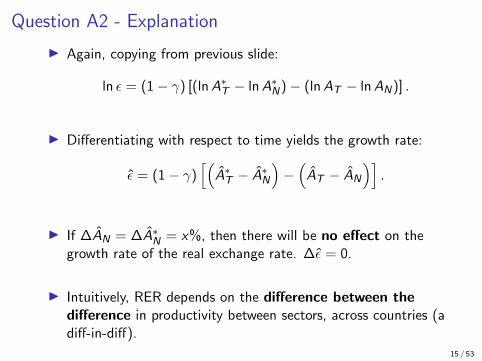
I Again, copying from previous slide:

ln ε = (1− γ) [(lnA∗T − lnA∗N)− (lnAT − lnAN)] .

I Differentiating with respect to time yields the growth rate:

ε = (1− γ)[(

A∗T − A∗N

)−(AT − AN

)].

I If ∆AN = ∆A∗N = x%, then there will be no effect on thegrowth rate of the real exchange rate. ∆ε = 0.

I Intuitively, RER depends on the difference between thedifference in productivity between sectors, across countries (adiff-in-diff).

15 / 53


I RER reflects the permanent productivity differences acrosscountries, and hence permanent income differentials.

I If productivity improves in both countries, no need for RERadjustment.

I What would be required for continual change in RER, ∆ε 6= 0?

I What is the Harrod–Balassa-Samuelson/Penn Effect?

16 / 53


I A3. When there is imperfect substitutability between domesticand foreign assets, an unanticipated increase in the domesticmoney supply could reduce the domestic nominal interest ratewhile keeping the nominal exchange rate fixed. True or false?Explain.

17 / 53

Question A3 - Short Answer

I This statement is true.

I Need to emphasise “could”.

18 / 53

Question A3 - Longer Answer I

I From lecture 8: consider the UIP condition extended toinclude a risk premium, denoted ρ:

i = i∗ +E [e]− e

e+ ρ.

I We have no model for how ρ behaves. Let’s invent one.

I Say ρ depends positively on level of bonds held by householdsρ = ρ(B − A)

+, where B is total supply and A are held by CB.

I Holding bonds leaves households more vulnerable to shocks.

I Under risk aversion, they require compensation for this.

19 / 53

Question A3 - Longer Answer II

I Following an unanticipated increase in the level of domesticmoney supply, there are now three distinct effects:

1. Standard expectations effect. (UIP shifts up).

2. Standard liquidity effect. (Move along UIP).

3. Additional risk premium effect. (New part).

I If supply unchanged, bonds held by households fall (B − A) ↓as the CB implements monetary expansion (by purchasingbonds using newly created reserves, as M ↑ infers A ↑).

I Given the above assumptions, the risk premium falls and UIPcurve shifts down.

I In principle, it is possible for the 3 to offset 1 and 2, suchthat M ↑ reduces i while leaving e unchanged.

I The statement is true.20 / 53

Question A3 - Graphical Answer I

I Start in equilibrium.

Money and FX Equilibrium

21 / 53

Question A3 - Graphical Answer II

I UIP shifts upwards due to Expectations Effect (EE).


22 / 53

Question A3 - Graphical Answer III

I Move along UIP due to Liquidity Effect (LE).


23 / 53

Question A3 - Graphical Answer IV

I UIP shifts downwards due to Risk Premium (RP).


24 / 53

Question A3 - Graphical Answer V

I Overall M ↑ could reduce i , but leave e unchanged.


25 / 53


I This seems unlikely. Not only must the change in riskpremium be large (offsetting both LE and EE), it must also doso perfectly.

I Generating an ad hoc off-model assumption for the behaviourof the risk premium enables us to freely move the UIPcondition where we like. Anything goes!

26 / 53

Long Questions

27 / 53

Question B1 - Set Up

I B1. Suppose the world consists of two countries, Home (H)and Foreign (F). There is perfect international capital mobilitybetween the two countries, H and F assets are perfectsubstitutes. The rate of return for a H investor on H and Fassets is Hs and Fs , respectively, where s = {1, 2} denotes thestate of nature. State 1 occurs with probability q and state 2with probability 1− q. The H investor allocates her wealth,W to max. expected utility:

U = qu(C1) + (1− q)u(C2).

where u(C ) = −e−C , and Cs = [αHs + (1− α)Fs ]W isconsumption in the state s, and α is the share of H assets inthe H investor’s portfolio. Suppose that W = 1, H1 = 3,H2 = 1, F1 = 1, F2 = 2, and q = 1/3.

28 / 53

B1 (a) - Rates of Return

I (a) Compare the expected rates of return on Home andForeign assets. How do they depend on the probability, q, ofstate 1?

I The expected return on each asset is calculated as the payoffin each state multiplied by its probability of occurring:

E [RH ] = qH1 + (1− q)H2 = 3q + 1− q = 2q + 1 =5

3,

E [RF ] = qF1 + (1− q)F2 = q + 2− 2q = 2− q =5

3.

I Given the calibration, this is 5/3 for both assets.

I Without calibrating q we observe:

dE [RH ]

dq= 2 > 0, while

dE [RF ]

dq= −1 < 0.

29 / 53

B1 (b) - Optimal Portfolio Allocation I

I (b) Derive the optimal portfolio share, α, from the first ordercondition. Explain intuitively whether it is desirable for theHome investor to engage in international portfoliodiversification.

I Consider the investor’s maximization problem:

maxα

qu(C1(α)) + (1− q)u(C2(α)),

s.t. Cs = [αHs + (1− α)Fs ]W , s = {1, 2}.

I The first derivative is:

dU

dα= qu′(C1)C ′1 + (1− q)u′(C2)C ′2,

where:C ′s = (Hs − Fs)W , s = {1, 2}.

30 / 53

B1 (b) - Optimal Portfolio Allocation II

I Using the functional form u′(C ) = e−C then gives:

qe−C1(H1 − F1)W + (1− q)e−C2(H2 − F2)W = 0.

I Using the calibrated values this becomes:

dU

dα= 2qe−1−2α − (1− q)eα−2 = 0.

I Rearranging we obtain the optimal level of α as:

2q

1− q= e3α−1,

2/3

2/3= e3α−1,

ln(1) = 3α− 1,

α = 1/3.

31 / 53

B1 (b) - International Diversification

I Though expected rates of returns are equal by construction,the optimal portfolio is diversified.

I This is beneficial because of the negative correlationbetween the return on Home and Foreign assets.

I International portfolio diversification allows consumptionsmoothing across states of nature.

I This is desirable as the consumer is risk averse, throughCARA utility function.

I Indeed with α = 13 the household fully smooths consumption

across states of nature (full insurance with C1 = C2 = 53).

32 / 53

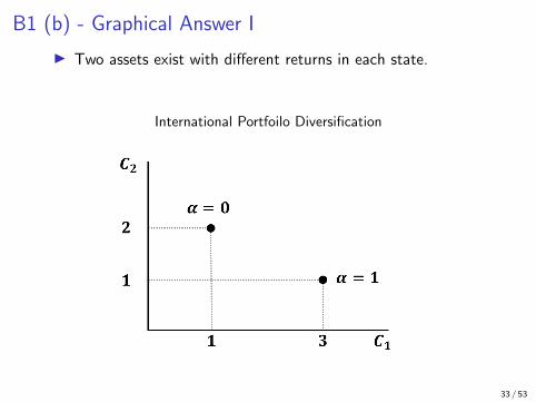
B1 (b) - Graphical Answer I

I Two assets exist with different returns in each state.

International Portfoilo Diversification

33 / 53

B1 (b) - Graphical Answer II

I Households may choose any portfolio of these assets.


34 / 53

B1 (b) - Graphical Answer III

I Alternatively if told α ∈ (0, 1) will have kinked budget line.


35 / 53

B1 (b) - Graphical Answer IV

I Concentrating wealth in either asset is sub-optimal.


36 / 53

B1 (b) - Graphical Answer V

I Better off to smooth consumption in each state.


37 / 53

B1 (c) - Changing Probabilities

I (c) Suppose now that the probability of state 1 increases.Explain how this would affect the optimal portfolio share, α,and the desirability of international portfolio diversification.

I The implications of q ↑ may be found by differentiating thesolution for optimal α (found earlier) with respect to q:

e3α−1 =2q

1− q,

3α− 1 = ln

[2q

1− q

],

α =1

3[ln(2q)− ln(1− q) + 1] ,

∂α

∂q=

1

3

[2

2q+

1

1− q

]=

1

3q(1− q)> 0.

38 / 53

B1 (c) - Intuition and Implications for Diversification

I As Pr(s = 1) = q ↑, then E [RH ] ↑ while E [RF ] ↓.I Allocation changes, as optimal to hold more H and less F.

I For some degree of diversification, without short-selling orleverage such that α ∈ (0, 1), the FOC becomes:

0 <1

3[ln(2q)− ln(1− q) + 1] < 1,

e−1 <2q

1− q< e2,

0.155 ≈ e−1

2 + e−1< q <

e2

2 + e2≈ 0.787.

I For q ∈ (0.155, 0.787), households will diversify portfolios.

I For q > 0.787 (q < 0.155), optimal to short F (H), if able to.

I If q very high then E [RF ] is so low, that risk-adjustedportfolio return is improved by borrowing F and investingabove W in H.

39 / 53

B1 (c) - Graphical Answer

I Changing q ‘tilts’ the utility curve, such that it may betangent at α = 1 (or α = 0).


40 / 53

Essay

41 / 53

Question C1 - Set Up

I C1. Are speculators irrational when they attack the currencypeg of a country that still has foreign exchange reserves?[Tripos 2001]

I No, speculators are not irrational when they attack a currencypeg of a country that still has foreign exchange reserves.

42 / 53

Question C1 - Longer Answer

I Lectures discuss three “generations” of currency crisis model.

1. Bad macro fundamentals (Latin-American crisis, 1980s).

2. Self-fulfilling crises (e.g., ERM crisis, 1992).

3. Financial fragility (e.g., South-East Asian crisis, 1997).

I Each has a role for rational speculation against the currencypeg, when foreign reserves are above zero.

43 / 53

Question C1 - Bad Macroeconomic Fundamentals

I Model due to Krugman (1979).

I Monetary financing of primary government deficits causeforeign reserves (F) to fall.

I When F = 0, currency peg e breaks and e moves freely.

I Shadow rate, eS , defined as the freely floating nominalexchange rate prevailing if CB held no foreign reserves.

I This would gradually depreciate as government deficitsfinanced by CB increasing money supply.

I A rational speculative attack arises when e = eS .

44 / 53

Question C1 - Generation I, Graph I

I If no speculative attack happens, Foreign reserves, F , fall untilF = 0. At this point e then follows eS .

Foreign Reserves and Exchange Rate

45 / 53

Question C1 - Generation I, Graph II

I But if investors hold domestic currency when F = 0 they facea sudden depreciation. So why hold it?


46 / 53

Question C1 - Generation I, Graph III

I Perfect foresight investors are better off selling Homecurrency to CB earlier (demanding Foreign reserves).


47 / 53

Question C1 - Generation I, Graph IV

I This forces Foreign reserves to deplete, F → 0, when e = eS .Afterwards the exchange rate follows eS .


48 / 53

Question C1 - A Unique Rational Equilibrium

I Why not attack earlier?

I If F = 0 before e = eS , the currency must appreciate to eS .

I Individual investors in Home currency would therefore notwish to sell during this attack (immediate capital loss).

I Better to wait, let others sell and e appreciate, then sellmyself.

I A last mover advantage exists, so nobody sells.

49 / 53

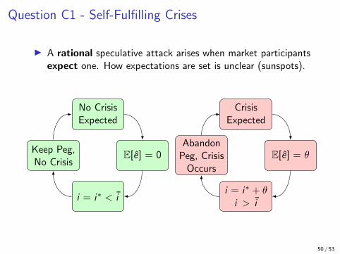
Question C1 - Self-Fulfilling Crises

I A rational speculative attack arises when market participantsexpect one. How expectations are set is unclear (sunspots).

No CrisisExpected

E[e] = 0

i = i∗ < i

Keep Peg,No Crisis

CrisisExpected

E[e] = θ

i = i∗ + θi > i

AbandonPeg, Crisis

Occurs

50 / 53

Question C1 - Financial Fragility

I Key point: Financial and currency crises are interrelated.

I E.g. Corsetti et al. (1999) and Burnside et al. (2001).

I No need for fiscal deficits, rising debt or falling reserves.

I Counting on future bailouts (moral hazard), a weaklyregulated financial sector engages in risky investment.

I News arrives of banking sector losses, and a monetaryfinanced government bailout (to satisfy solvency issues).

I Banking failure contagion to government balance sheet.

I A rational speculative attack arises as investors expectinflation and an overvalued exchange rate (M ↑⇒ P ↑, e ↑).

51 / 53

Next Class

52 / 53

Next Class

I Revision session discussing answers from mock exam.

I After econometrics project.

53 / 53

part iia supervision 9 - international economics ii

Documents