part ii mathematical biology - lent 2017 · 2019-10-18 · t c ermission 1 deterministic systems,...
TRANSCRIPT

Cop
yri
ght
c ©20
19U
niv
ersi
tyof
Cam
bri
dge
.N
otto
be
quot
edor
repro
duce
dw
ithou
tp
erm
issi
on
Part II Mathematical Biology - Lent 2017
Lecturer: Prof. Julia Gog ([email protected])
(this version September 2019 - some typos corrected)
Contents
0 Introduction 3
1 Deterministic systems, no spatial structure 5
1.1 Single population models . . . . . . . . . . . . . . . . . . . . . . . . . . 5
1.1.1 Simple birth and death models . . . . . . . . . . . . . . . . . . . 5
1.1.2 Delay models . . . . . . . . . . . . . . . . . . . . . . . . . . . . . 8
1.1.3 Populations with age structure . . . . . . . . . . . . . . . . . . . 19
1.2 Discrete time . . . . . . . . . . . . . . . . . . . . . . . . . . . . . . . . . 25
1.2.0 Revision: 1-D stability in difference equations (maps) . . . . . . 25
1.2.1 The logistic map . . . . . . . . . . . . . . . . . . . . . . . . . . . 26
1.2.2 Higher order discrete systems . . . . . . . . . . . . . . . . . . . 30
1.3 Multi-species models . . . . . . . . . . . . . . . . . . . . . . . . . . . . . 35
1.3.0 Revision: 2-D stability in continuous time . . . . . . . . . . . . . 35
1.3.1 Competition models . . . . . . . . . . . . . . . . . . . . . . . . . 36
1.3.2 Predator-prey models . . . . . . . . . . . . . . . . . . . . . . . . 40
1.3.3 Chemical kinetic models . . . . . . . . . . . . . . . . . . . . . . . 46
1.3.4 Epidemic models . . . . . . . . . . . . . . . . . . . . . . . . . . . 50
1.3.5 Excitable systems . . . . . . . . . . . . . . . . . . . . . . . . . . 59
1

Cop
yri
ght
c ©20
19U
niv
ersi
tyof
Cam
bri
dge
.N
otto
be
quot
edor
repro
duce
dw
ithou
tp
erm
issi
on
2 Stochastic systems 64
2.0 Preliminaries . . . . . . . . . . . . . . . . . . . . . . . . . . . . . . . . . 64
2.0.0 Revision: discrete probabilities and generating functions . . . . . 64
2.0.1 Why bother? . . . . . . . . . . . . . . . . . . . . . . . . . . . . . 65
2.0.2 The first step . . . . . . . . . . . . . . . . . . . . . . . . . . . . . 66
2.1 Discrete population sizes . . . . . . . . . . . . . . . . . . . . . . . . . . 68
2.1.1 Single populations . . . . . . . . . . . . . . . . . . . . . . . . . . 68
2.1.2 Extinction . . . . . . . . . . . . . . . . . . . . . . . . . . . . . . . 77
2.1.3 Multiple populations . . . . . . . . . . . . . . . . . . . . . . . . . 80
2.2 Continuous population sizes . . . . . . . . . . . . . . . . . . . . . . . . . 84
2.2.1 Fokker-Planck for a single variable . . . . . . . . . . . . . . . . . 84
2.2.2 Multivariate Fokker-Planck . . . . . . . . . . . . . . . . . . . . . 88
3 Systems with spatial structure 97
3.0 Preliminaries . . . . . . . . . . . . . . . . . . . . . . . . . . . . . . . . . 97
3.1 Diffusion and growth . . . . . . . . . . . . . . . . . . . . . . . . . . . . . 99
3.1.1 Linear diffusion in finite domain . . . . . . . . . . . . . . . . . . . 99
3.1.2 Linear diffusion in infinite domain . . . . . . . . . . . . . . . . . . 103
3.1.3 Nonlinear diffusion . . . . . . . . . . . . . . . . . . . . . . . . . . 112
3.2 Travelling waves in reaction-diffusion systems . . . . . . . . . . . . . . . 116
3.2.0 General F . . . . . . . . . . . . . . . . . . . . . . . . . . . . . . . 116
3.2.1 Fisher’s equation . . . . . . . . . . . . . . . . . . . . . . . . . . . 117
3.2.2 Bistable systems . . . . . . . . . . . . . . . . . . . . . . . . . . . 126
3.3 Spatial instabilities . . . . . . . . . . . . . . . . . . . . . . . . . . . . . . 130
3.3.1 Chemotaxis . . . . . . . . . . . . . . . . . . . . . . . . . . . . . . 130
3.3.2 Turing instabilities . . . . . . . . . . . . . . . . . . . . . . . . . . 135
2

Cop
yri
ght
c ©20
19U
niv
ersi
tyof
Cam
bri
dge
.N
otto
be
quot
edor
repro
duce
dw
ithou
tp
erm
issi
on
0 Introduction
Acknowledgements
Much of the content and the starting point for these notes comes from Prof. PeterHaynes’s version of the notes from 2012. Any typos or errors are, however, likely to bethe fault of this author.
Practicalities
This are intended as archived version of the notes from the Part II Mathematical Biologycourse, as lectured by me (Julia Gog) in Lent 2017, within Part II of the MathematicalTripos, University of Cambridge. For Part II students in future years, these notes mightbe useful as an extra resource perhaps for reading ahead over the summer, but pleasedo not use them as a replacement for attending lectures or working from the presentlecturer’s resources. Lectures are good, you should go to them: you’ll always learn abit more, see something in a different way or build more intuition for what is really goingon.
There are exercises in green boxes throughout these notes. These were set in lecturesand intended as being additional to the usual examples sheets. These exercises shouldbe fairly doable without any help from a supervisor, and I recommend doing them asyou work through the notes. There exist a full set of ‘solutions’: you might find thesewherever you found these notes: these can be used to check you are working alongthe right lines, or to see what was intended.
For anyone who uses the notes, I hope these notes are interesting and useful. Mostof all, I hope they inspire you to explore mathematical biology further. If you have anycomments or corrections, please do email me: [email protected]. I might not respondimmediately (or at all, sorry!), but feedback will be useful in updating and amendingthese for future use.
Preparation for this course
Part II Dynamical Systems is ‘helpful’ for parts of this course but certainly not essen-tial. If you did not do Dynamical Systems, then it might be wise to do a little revisionof parts of Ia Differential Equations: stability of equilibria of discrete and continuoustime systems (Jacobians, saddles/focus/node, phase-plane diagrams). Indeed ‘Ordi-nary Differential Equations’ by Robinson (see schedules for Ia Differential Equations)chapters 32 and 33 (‘coupled nonlinear equations’ and ‘ecological models’) will put youright on track for this course. The middle part of the course on stochastic systems willuse some knowledge from Ia Probability, including generating functions. It would be a
3

Cop
yri
ght
c ©20
19U
niv
ersi
tyof
Cam
bri
dge
.N
otto
be
quot
edor
repro
duce
dw
ithou
tp
erm
issi
on
good idea to revise separable solutions from Ib Methods for the last part of the courseon diffusion.
Interesting reading
None of these are essential to follow this course, but should be of interest:
• J.D. Murray Mathematical Biology (3rd edition) (see schedules) - the classic texton mathematical biology, covering a range of applications
• D. Neal Introduction to Population Biology - much overlap with this course inmathematical detail, but explores the biological principles in rather more depthand includes many real examples. Should be completely readable by you duringor after this course.
• Mathematics is biology’s next microscope, only better; Biology is mathematics’next physics, only better - article by Joel E. Cohen in PLoS Biology 2004 DOI:10.1371/journal.pbio.0020439
4

Cop
yri
ght
c ©20
19U
niv
ersi
tyof
Cam
bri
dge
.N
otto
be
quot
edor
repro
duce
dw
ithou
tp
erm
issi
on
1 Deterministic systems, no spatial structure
1.1 Single population models
1.1.1 Simple birth and death models
The simplest model?
Let x(t) be population size as a function of time t. Assume that the number of offspringproduced per individual per unit time is a constant b > 0. Similarly assume that thedeath rate (number of deaths per unit time per individual) is a constant d > 0.
x(t+ δt) = −x(t) + b x δt− d x δt
Divide by δt and take the limit as δt→ 0.
dx
dt= (b− d)x = rx where r = b− d.
Solution is x(t) = x0ert, where x(0) = x0, so the population grows indefinitely if r > 0
and decays towards zero (implying extinction) if r < 0.
Exercise 1: In the case when r < 0, find the half-life of the population
Exercise 2: Actually, this simple model is pretty good for invasions of new pop-ulations. Suppose a new disease is discovered and there are 1000 cases lastweek and 1500 cases this week, roughly when did the disease first appear?
Note that in a deterministic system, only the difference between b and d matters,e.g. b = 21, d = 20 gives entirely the same dynamics as b = 1, 000, 001, d = 1, 000, 000.These will differ in an analogous stochastic model (the ones with higher rates will fluc-tuate wildly).
Birth and death rates depend on population size Rather than constant, allowthe number of offspring per individual per unit time to depend on population size, a(x),and similarly the death rate b(x). Then we have:
dx
dt= [b(x)− d(x)]x
5

Cop
yri
ght
c ©20
19U
niv
ersi
tyof
Cam
bri
dge
.N
otto
be
quot
edor
repro
duce
dw
ithou
tp
erm
issi
on
Again, only the difference between birth and death rates matter in the deterministicsystem.
Typically, one might expect the birth rate per capita to decrease and/or death rate toincrease for very large population size, as resources become scarce. For examplehere we could take the birth rate to be constant (b(x) = B) and the death rate to beproportional to population size (d(x) = Dx):
dx
dt= [B −Dx]x
By rescaling the population size and renaming parameters, we have the logistic equa-tion:
dx
dt= αx(1− x)
Exercise 3: Find the rescaling.
For x < 1, births outnumber the deaths and the population grows. For x > 1, theopposite occurs and the population shrinks. The equilibrium population size (scaled) isone.
The logistic model
dx
dt= αx(1− x)
This is easy to solve:
∫1
x(1− x)dx =
∫1
x+
1
1− xdx = log
∣∣∣∣ x
1− x
∣∣∣∣+ C = αt
So putting x = x0 at t = 0 we have:
x
1− x=
x0
1− x0
eαt
Which rearranges to:
x =x0e
αt
(1− x0) + x0eαt
6

Cop
yri
ght
c ©20
19U
niv
ersi
tyof
Cam
bri
dge
.N
otto
be
quot
edor
repro
duce
dw
ithou
tp
erm
issi
on
Reassuringly, our steady population size is there: x0 = 1 gives x(t) = 1. Also, it isalways sensible to check zero initial conditions: x0 = 0 gives x(t) = 0.
Exercise 4: show that the solution to the logistic equation can be rewritten forsome t0 as:
x =
12
+ 12
tanh(
12α(t− t0)
)for x0 < 1
12
+ 12
coth(
12α(t− t0)
)for x0 > 1
Note that for positive initial population size (x0 > 0), x → 1 as t → ∞ (from above ifx0 > 1 and from below if x0 < 1). There is a stable equilibrium, achieved for all positiveinitial conditions. The zero equilibrium x = 0, b is unstable.
One-dimensional stability recap
Consider:
dx
dt= f(x)
The steady-states are the values of x∗ for which f(x∗) = 0. These may be interchange-ably referred to as equilibria, fixed points, steady states or constant solutions. Stabilityis determined by behaviour near the fixed point, which can be found by linearisationaround x∗. Set x(t) = x∗ + ε(t). Then:
dx
dt=dε
dt= f(x∗ + ε) = f(x∗)︸ ︷︷ ︸
=0
+εf ′(x∗) +O(ε2)︸ ︷︷ ︸ignore
Hence:
dε
dt' f ′(x∗)ε which has solution ε(t) ' ε0 exp[f ′(x∗)t].
So ε, the perturbation away from x∗ grows if f ′(x∗) > 0 (unstable) and shrinks if f ′(x∗) <0 (stable).
In practice, just check sign of f ′ at fixed points. For simple biological models, this canusually be done easily by plotting f .
Exercise 5: check stability of the fixed points of the logistic model
7

Cop
yri
ght
c ©20
19U
niv
ersi
tyof
Cam
bri
dge
.N
otto
be
quot
edor
repro
duce
dw
ithou
tp
erm
issi
on
1.1.2 Delay models
So far, we have x′(t) depending on x(t), i.e. the instantaneous current population size.Of course this is not always realistic. For example, offspring are not really producedinstantaneously, there may be a significant gestation period, or time for eggs to hatch.Even then, new offspring may need further time to mature to adulthood, before they canin turn produce offspring. So, we might want x(t) to denote adults, and births and/ordeaths may depend on the population size at some past time point. In physiologicalmodels, there is often some form of delay, for example heart rate does not respondinstantly to exercise. In biochemical signalling, there can be many steps between atrigger and effect, which can sometimes be modelled relatively simply as a time lag. end of
lecture 1Mathematically, this leads to delay-differential equations (DDEs). Here is an example,the Hutchinson-Wright equation, which can be viewed as an extension to the logisticequation:
dx
dt= αx(t) [1− x(t− T )]
where the delay time T is a new parameter in the model (assume T > 0, note T = 0was logisitic equation).
We can analyse its dynamics with much the same ideas as before: find the interestingfixed points and look at their stability by considering a small perturbation. Clearly x(t) =1 is still the non-trivial steady state. Now set x(t) = 1 + ε(t) and sub in:
dε
dt= α(1 + ε(t))(−ε(t− T ))
dε
dt= −αε(t− T ) +O(ε2)
And drop O(ε2) from here.
This is still linear, so reasonable to seek a solution of the form ε = ε0est:
s = −α e−sT (1)
We would like know the solutions for s. We see that if T = 0, then this just returnss = −α, which corresponds to the stable fixed point of the logistic equation. If T > 0,then we need to look a bit more carefully.
First we might reasonably seek real s solutions. Rearranging:
sTesT = −αT
8

Cop
yri
ght
c ©20
19U
niv
ersi
tyof
Cam
bri
dge
.N
otto
be
quot
edor
repro
duce
dw
ithou
tp
erm
issi
on
Consider the shape of the LHS as a function of sT . It has a single minimum at sT = −1when the LHS is equal to −e−1. So, there are negative real roots for αT < e−1 and noreal roots otherwise.
-1�
-e-1
�(�) = � ��
If we look at the solution near sT = 0, for small αT , the gradient is approximately 1, sowe have sT ≈ −αT so this is a continuation of the solution s = −α, which is what wewould have got with the logistic equation.
So far we have only considered real roots for s, but we might (correctly) suspect therecould be complex roots of 1 for s. What would this mean? Our perturbation wouldfollow ε0e
st, so a complex solution would just give a solution that grows or decays butwith oscillations (think back to complimentary functions in second order linear ODEs).We are now interested in the sign of the real part of s. If Re(s) > 0 we say it is unstable,if Re(s) < 0 we say it is stable. It is not usually possible to solve explicitly for s, but wecan see now that it would be sensible to find when stability might change, i.e. Re(s) = 0.
Now lets seek complex roots of (1) by setting s = σ + iω (where σ and ω are the realand imaginary parts of s). Sub in:
σ + iω = −αe−sσe−isω = −αe−sσ [cos(ωT )− i sin(ωT )]
Take real and imaginary parts:
σ = −αe−σT cos(ωT ) real part
ω = +αe−σT sin(ωT ) imaginary part
Seek a solution with σ = 0. Things simplify quite a bit:
0 = −α cos(ωT )
ω = +α sin(ωT )
Squaring and adding gives ω2 = α2 so ω = ±α. This is not too surprising: we shouldexpect complex conjugate pairs of solutions. Could limit calculuations to ω > 0 ifit helped, and just remember the complex conjugates are also there. In any case,subbing in either solution to the second equation, gives the same outcome:
9

Cop
yri
ght
c ©20
19U
niv
ersi
tyof
Cam
bri
dge
.N
otto
be
quot
edor
repro
duce
dw
ithou
tp
erm
issi
on
sin(αT ) = 1 so αT =π
2,5π
2,9π
2, . . .
and no need to worry about negative solutions, as both α > 0 and T > 0. So thinkingabout increasing T up from zero, we have a complex root switch real part sign manytimes. We are interested in the first one: αT = π/2.
This is optional, but as this is the first example, we will check that we really do havestable solutions when 0 < T < π
2α. It turns out to be sensible to split into two cases
according to modulus of ω
• For |ω| > α, from considering modulus in the equation for the real part we seethat exp(−σT ) > 1 hence σ < 0.
• For |ω| ≤ α, |ωT | ≤ αT < π/2 so cos(ωT ) > 0. From the equation for the realpart, we see σ < 0 again.
So either way, we have negative σ and hence stable solutions. Note we have notactually found any values for s, but we have shown they will have negative real part inthis range.
Numerical simulation is consistent with 0 < T < 1αe
solutions decay exponentially tothe fixed point; for 1
αe< T < π
2αsolutions decay and oscillate to the fixed point, and for
T > π2α
the solution is unstable and heads to a cycle. This is typical: delay-differentialequation models often lead to oscillatory solutions.
0 10 20 30 40����0.0
0.5
1.0
1.5
2.0
2.5
3.0�
T = 0.3 α=1
0 10 20 30 40����0.0
0.5
1.0
1.5
2.0
2.5
3.0�
T = 1.2 α=1
0 10 20 30 40����0.0
0.5
1.0
1.5
2.0
2.5
3.0�
T = 1.55 α=1
0 10 20 30 40����0.0
0.5
1.0
1.5
2.0
2.5
3.0�
T = 1.8 α=1
(See Mathematica: Delay Logistic Equation)
10

Cop
yri
ght
c ©20
19U
niv
ersi
tyof
Cam
bri
dge
.N
otto
be
quot
edor
repro
duce
dw
ithou
tp
erm
issi
on
Under the carpet
Treat this note as starred. If you are happy with DDEs already, then skip it. If you areconcerned that something might have been swept under the carpet here, you are right,so read on. What we have actually done is
• Found where there are real solutions for s and shown they are negative.
• For first range of T showed that any solution for s has negative real part
• Found all the values of T > 0 where a solution has real part zero
We can actually know more about the solutions for s of sTesT = −αT if we read up on‘Lambert W-Functions’. There are many solutions. Mathematica has a built-in functionthat can be used to give them numerically, and we can plot their real part as a functionof T (set α = 1 for simplicity).
π
2π 3π
22π 5π
23π 7π
24π 9π
25π
T
-3.0
-2.5
-2.0
-1.5
-1.0
-0.5
σ
π
2π 3π
22π 5π
23π 7π
24π 9π
25π
T
-0.10
-0.05
0.05
0.10
0.15
σ
σ = Re(s) against T for α = 1 for top 10 solutions(same plot each side, just different vertical scale)
The root with the largest real part (top line on graph) actually corresponds to that largestreal solution to start with, and you can see the sharp change of direction as it becomescomplex. The vertical zoom-in on the right shows more clearly that successive (pairsof) solutions pass upwards into positive σ.
For T = 0 we only had one value of s (namely s = −α). This was enough to determinethe linear behaviour of any small perturbation: ε = ε0 exp (−αt), and we’d just need toput in the appropriate single constant ε0. Now, for a perturbation, we should specify notjust ε(0) but also ε(t) for the interval t ∈ [−T, 0]. And the resultant dynamics will be asa sum of these types of solution with different s:
ε(t) =∑i
aiesit
11
Cop
yri
ght
c ©20
19U
niv
ersi
tyof
Cam
bri
dge
.N
otto
be
quot
edor
repro
duce
dw
ithou
tp
erm
issi
on
where the ai are determined by the initial conditions. The si with the largest real partwill end up dominating as t increases.
So, actually we have got the dynamics right from the simple approach we first took: thereal solution dominated when it existed, the we had an oscillatory but decaying solutionuntil we found the lowest T where things could lose stability. For math bio, treat thissimple approach as sufficient.
Be a bit careful when rescaling DDEs
This is just a word of caution about rescaling delay differential equations with respectto time. In short, you must remember to rescale any time lag also. In long, we will usethe above as an example:
dε(t)
dt= −αε(t− T )
There are two parameters here, α and T . It is tempting to try and get rid of α byrescaling time. We set t = αt to cancel out with the α:
dε(t)
dt= α
dε
dt= −αε(t− T )
so
dη(t)
dt= −ε(t− T ) = −η(α(t− T )) = −η(t− αT )
and finally:dη(t)
dt= −η(t− αT ).
So really we have not eliminated α but we have compounded our two parameters to asingle parameter combination αT .
In general, be aware that the lag needs to rescale with time also. It is not usual inpractice to write out all of these steps. It is usually acceptable to reuse the originalvariable name (ε here), but the change was made explicit just this once.
Exercise 6: Find the equivalent of equation (1) for this rescaled DDE. (It turnsout to be slightly different, but it ought to give us the same conditions for stabil-ity.)
12

Cop
yri
ght
c ©20
19U
niv
ersi
tyof
Cam
bri
dge
.N
otto
be
quot
edor
repro
duce
dw
ithou
tp
erm
issi
on
DDE Example: Blowflies
This example stems from classic experimental work by Nicholson and others in the1950s on the Australian sheep blowfly. Populations of flies were kept in the lab andpopulation size was tracked over time, showing some quite spectacular fluctuationsdespite the available food and other external factors being kept steady. The full lifecycle of these flies is a few weeks (eggs, larval stages, then adult). Mathematicalbiologists have modelled this using delay differential equations.
The unusual thing here is that the number of eggs produced by adult flies is verystrongly regulated by population size, in fact we assume that the per capita rate of eggproduction is exponentially decreasing with population size. This means that the totalnumber of eggs produced is no longer monotonic increasing with population size, butnow is unimodal with a peak at x = x0. end of
lecture 2Per capita egg production if population has size x: Pe−x/x0
Total egg production from population of size x: p(x) = Pxe−x/x0
x0�
����� ����
Now assume that eggs turn into adults after a delay tD, and that the per capita deathrate δ does not depend on population size, and we have our model:
dx(t)
dt= P x(t− tD)Exp
(− 1
x0
x(t− tD)
)︸ ︷︷ ︸
new eggs at time t−tD
− δ x(t)︸ ︷︷ ︸death
(2)
Note that x(blah) denotes x evaluated at blah (as opposed to multiplied by), and simi-larly for x below.
This system has four parameters1: P , tD, x0 and δ. By strategic rescaling, this can bereduced to two. As usual, we can rescale time to adsorb a parameter, and here we’llchoose the death rate. Set t = δ × t to make d
dt= δ d
dt.
We can also rescale x to tidy the exponent: set x = x/x0 . We will consider x as a
1and as usual in mathematical biology, assume everything is positive unless you have a good reasonto think otherwise
13

Cop
yri
ght
c ©20
19U
niv
ersi
tyof
Cam
bri
dge
.N
otto
be
quot
edor
repro
duce
dw
ithou
tp
erm
issi
on
function in our rescaled time: t. So we are setting this
x(t) = x0 x(t)
= x0 x (δ t ) ,
so in particularx(t− tD) = x0 x (δ × (t− tD)) = x0 x
(t− δ tD
).
Hence making these changes and also dividing through by x0:
dx(t )
dt=P
δx(t− δ tD)e−x(t−δ tD) − x(t )
From this we can see that the model really only depends on two parameter combina-tions. Set a = δtD and b = PtD (turns out to be sensible to think of them both asincreasing in tD, so use these and then drop the hats to get the system in a suitableform to analyse:
dx(t)
dt=b
ax(t− a) e−x(t−a) − x(t) (3)
Exercise 7: get from equation 2 to equation 3 (without using notes!)
To find any equilibria, we solve for x(t) = x∗ where x∗ is constant:
0 =b
ax∗e−x
∗ − x∗
Which gives x∗ = log ba
as the non-trivial solution. Assume b > a so that this solution ispositive.
For stability, look at dynamics close to this fixed point, i.e. ε small2:
x(t) = x∗ + εy(t)
Sub this into equation 3:
ε y′(t) =b
a(x∗ + ε y(t− a)) e−x
∗︸︷︷︸=a/b
e−ε y(t−a) − (x∗ + ε y(t)))
= (x∗ + ε y(t− a)) e−ε y(t−a) − (x∗ + ε y(t))
= (x∗ + ε y(t− a)) (1− ε y(t− a))− (x∗ + ε y(t)) +O(ε2)
2We don’t really need ε and y(t) (lectures just used ε(t)). Just need some function of time which isassumed to be small, but sometimes it is easier to put ε in as a constant to explicitly to keep track ofwhat is small.
14

Cop
yri
ght
c ©20
19U
niv
ersi
tyof
Cam
bri
dge
.N
otto
be
quot
edor
repro
duce
dw
ithou
tp
erm
issi
on
And the order 1 terms cancel (which is reassuring, as it was supposed to be a fixedpoint) and then taking just order ε:
y′(t) = (1− x∗) y(t− a)− y(t)
Exercise 8: Continue from here to get to:
σ = (1− x∗) e−aσ cos(aω)− 1
ω = (1− x∗) e−aσ(− sin(aω)) .
Exercise 9: Show the system is stable for b < e2a.
0 20 40 60 80 100����0.0
0.5
1.0
1.5
2.0
2.5
3.0�����
a = 5 b=40
0 20 40 60 80 100����0
1
2
3
4
�����a = 5 b=60
0 20 40 60 80 100����0
1
2
3
4
5
6
7
�����a = 5 b=100
0 20 40 60 80 100����0
2
4
6
8
10
�����a = 7 b=200
(See Mathematica: Blowflies, and keep b� a)
15

Cop
yri
ght
c ©20
19U
niv
ersi
tyof
Cam
bri
dge
.N
otto
be
quot
edor
repro
duce
dw
ithou
tp
erm
issi
on
Physiological Example: Breathing
This is a simple model of respiration (breathing) where we focus on one particularfunction of breathing: to remove carbon dioxide from the blood. We assume thereis a feedback system where the volume of breath depends positively on the level ofcarbon-dioxide in the blood.
V = air inhaled (per breath)
C(t) = concentration of carbon dioxide in the blood at time t
And we use a Hill3 function to model how V depends on C:
V (C) = VmaxCm
am + Cm
a�
Vmax/2
Vmax
�
Hill function for various m: red m = 1/2, black m = 1, blue m = 2. They all pass thoughthe same point at C = a: half of the maximum Vmax.
However, there will be a lag between the level of carbon dioxide being detected and thetime until the breath volume is adjusted. This will involve a series of chemical reactions,and communication with the brainstem, but we do not need to know all the details, justthat there is some time difference, call it T . Also assume that the amount of carbondioxide breathed out is proportional both to its current concentration and to the breathvolume, with multiplicative constant b. Finally, assume that carbon dioxide in the bloodis added at a constant rate p (from other physiological processes around the body).This gives us the folioing equation:
3Archibald Hill 1886-1977: Trinity mathmo and Nobel Prize winning Physiologist, among many otherthings: http://www.nobelprize.org/nobel_prizes/medicine/laureates/1922/hill-bio.html
16

Cop
yri
ght
c ©20
19U
niv
ersi
tyof
Cam
bri
dge
.N
otto
be
quot
edor
repro
duce
dw
ithou
tp
erm
issi
on
dC
dt= +p︸︷︷︸
CO2 in to blood
−bC(t)V (C(t− T ))︸ ︷︷ ︸breathed out
= p −bC(t)VmaxC(t− T )m
am + C(t− T )m
end oflecture 3And we go ahead and rescale in the same way as before. We can pick up a good
rescaling for C by tidying the Hill function: set C = C/a. Again, we can choose toeliminate something else by rescaling time, so go for making that first term into 1. Sett = p
at so that d
dt= p
addt
:
dC
dt= 1− abVmax
pC(t )
C(t− pT/a)m
1 + C(t− pT/a)m
Again, note how the time lag also is rescaled as we are now working with C as afunction of t. Now we can see there are essentially two new parameter combinationsemerging here, τ = pT/a and α = abVmax/p, so work in terms of those and also we candrop the hats at this point4:
dC
dt= 1− αC(t)
C(t− τ)m
1 + C(t− τ)m
This could be tidied a little further by defining f(x) = xm/(1 + xm):
dC
dt= 1− αC(t)f(C(t− τ))
Seek a constant equilibrium solution:
0 = 1− αC∗f(C∗)
1 = αC∗f(C∗)
The function f increases from zero to one. While we can’t write down an explicit solu-tion for this (at least not for general m in the Hill function), we can easily see that theright-hand side is unboundedly monotonically increasing, starting from zero, so therewill be a unique solution C∗. Also, as f < 1 we know that C∗ will satisfy C∗ > 1/α,which will turn out to be useful later.
For stability, as usual we set C = C∗ + εy(t).4in lectures, we just reused T , but done with τ here
17

Cop
yri
ght
c ©20
19U
niv
ersi
tyof
Cam
bri
dge
.N
otto
be
quot
edor
repro
duce
dw
ithou
tp
erm
issi
on
εy′(t) = 1− α (C∗ + εy(t))f(C∗ + εy(t− τ))
= 1− α (C∗ + εy(t)) (f(C∗) + εy(t− τ)f ′(C∗)) +O(ε2)
= 1− α [C∗f(C∗) + εy(t)f(C∗) + C∗εy(t− τ)f ′(C∗)] +O(ε2)
= 1− αC∗f(C∗)︸ ︷︷ ︸=0
−εα[y(t)f(C∗) + C∗y(t− τ)f ′(C∗)] +O(ε2)
And so to order ε (in other words, linearising):
y′(t) = −αf(C∗)︸ ︷︷ ︸A
y(t)− αC∗f ′(C∗)︸ ︷︷ ︸B
y(t− τ)
for some constants A and B.
Exercise 10 : show that
A =1
C∗, B =
(1− 1
αC∗
)m
C∗.
and check that B is positive
So, in essence:y′(t) = −Ay(t)−By(t− τ)
Now we have an equation which is linear in y, though it is still a delay equation, so wetry a solution of the form y = est:
s = −A−Be−sτ
We can immediately see that for τ = 0 that s = −A − B, so C∗ is stable. For moregeneral parameters, we explore this as usual by setting s = σ + iω (where we alwaystake σ and ω to be real).
σ = −A−Be−στ cosωτ
ω = Be−στ sinωτ
Note that the equations are symmetric in ±ω, which is not surprising: the roots for sshould be in complex conjugate pairs. We could restrict attention to ω > 0.
There’s a few things we could argue through now. With a bit of work, we could showfor small τ (actually not very small needed), we should show σ > 0 impossible, so stillstable.
Actually, we might be interested in the shape parameter of the Hill function m. We canshow that if m is small, then B will be small (need to be a bit careful as m is implicitly
18

Cop
yri
ght
c ©20
19U
niv
ersi
tyof
Cam
bri
dge
.N
otto
be
quot
edor
repro
duce
dw
ithou
tp
erm
issi
on
in c∗, but that can be bounded). If B is small, we can also see σ > 0 impossible. Nowthink about larger m, as it increases from small. To try and find a boundary when thereal part goes through zero (which should give us the edge of instability), set σ = 0:
0 = −A−B cosωτ
ω = B sinωτ
Which rearranges to:
−Aτ tan(ωτ) = ωτ (4)B2 = bA2 + ω2 (5)
Equation 4 has a root for ωT in (π/2, π), and its exact value will depend on Aτ . Call itg(Aτ). There are other roots further on, but this lowest one turns out to be the one ofinterest. Equation 5 gives an implicit expression that must be satisfied by A, B and τ :
B2 = A2 + τ−2g(Aτ)2
Exercise 11: Consider varying the parameter m. Show that this boundary forinstability means that:
1 +π2C∗2
4τ 2≤ m2
(1− 1
αC∗
)2
≤ 1 +π2C∗2
τ 2
And in particular, this means that this critical m is greater than 1.
1.1.3 Populations with age structure
So far, we have just been considering the population size (usually x). However, whenthinking about birth and death rates, it would often be important to consider the age ofindividuals. Now, set n(a, t) to be the number of individuals at time t who are age a 5.The total population at time t can be found by integrating over all ages:
N(t) =
∫ ∞0
n(a, t)da
Now we set up birth and death rates as functions of age. Let b(a) be the birth rate fromindividuals of age a. Let µ(a) be the death rate of individuals of age a.
5Strictly, this is a density function in a. So this should really be n(a, t)δa is the number of individualsaged between a and a+ δa. We don’t usually need to say all of this though.
19

Cop
yri
ght
c ©20
19U
niv
ersi
tyof
Cam
bri
dge
.N
otto
be
quot
edor
repro
duce
dw
ithou
tp
erm
issi
on
�(�)
μ (�)
���
Example for b(a) and µ(a). Birth rate might be highest from a particular age group, whilethe death rate may increase with age.
Now start to build the equations that govern n. Consider how a chunk6 of populationages as time increases from t to t + δt. They will age by δt, but a small number mighthave die in that time:
n(a+ δt, t+ δt) = n(a, t)− µ(a)δt n(a, t) +O(δt2) (6)
The left hand side can be expanded by Taylor series, again to first order in δt:
n(a+ δt, t+ δt) = n(a, t) + δt∂n
∂a(a, t) + δt
∂n
∂t(a, t) +O(δt2)
Sub this in to equation 6, cancel the n(a, t), divide by δt and take limit δt→ 0:
∂n
∂t(a, t) +
∂n
∂a(a, t) = −µ(a)n(a, t)
Or we usually write:
∂n
∂t+∂n
∂a= −µ(a)n(a, t) (7)
With an initial condition in time, this is most of the story, but we also need a boundarycondition in age, i.e. the newborns that appear at age zero:
n(0, t) =
∫ ∞0
b(a)n(a, t)da (8)
6c.f. fluids courses where we start with a blob of fluid. In fact this derivation is very similar if wereplace space with age. The material derivative in fluids ( D
Dt = ∂∂t + u. ∂∂x ) is like the left hand side in
equation 7 if we think about age rather than space, and our blob moves (ages) with velocity 1 in time.Note: don’t try to think too hard about a fluids equivalent for the the boundary condition at age 0: thatwould be taking the analogy too far!
20
Cop
yri
ght
c ©20
19U
niv
ersi
tyof
Cam
bri
dge
.N
otto
be
quot
edor
repro
duce
dw
ithou
tp
erm
issi
on
The age ∞ might look worrying, but in practice for any sensible model, the birth ratetimes population size is zero for a greater than some age, or at least mathematicallythe product tends to zero sufficiently fast for this integral to always be sensible.
Wave-like solutions
(Note: would be a good idea to have read through this once and understood the ideas,but otherwise treat it as starred)
The left hand side of equation 7 may remind you of characteristic or wave solutionsfrom earlier courses (such as IB Methods). This works very easily for µ(a) = 0 andignoring age boundary condition. Any general function of n(a, t) = g(a − t) solves∂n∂t
+ ∂n∂a
= 0. This would be just a fixed population age distribution, just drifting upwardsin age with time (which is fine only for no deaths).
We can extend this to account for the age-dependent death rate, and it can easily bechecked that equation 7 is solved by:
n(a, t) = Exp
[−∫ a
0
µ(s)ds
]g(a− t)
The exponential term represents the probability of surviving to age a, where s is adummy variable for age in the integration. We don’t know much about g yet. This againis a wave-like solution, with some decay with age to account for deaths.
If we are given an initial condition i.e. n(a, 0) = n0(a) then that is enough to specify g(x)for x > 0:
n(a, 0) = n0(a) = e−∫ a0 µ(s)dsg(a)
⇒ g(a) =n0(a)
e−∫ a0 µ(s)ds
Effectively, this is working out the number of births at time a ago, by consider those agea and scaling it up to account for the proportion that died before time zero.
To determine g(x) for x < 0, we should use the newborn boundary condition (equation8), which gives:
g(−t) =
∫ ∞0
b(a)e−∫ a0 µ(s)dsg(a− t)da
And then split integral range at a = t so when a − t changes sign so we can use theinitial condition in the second term:
21

Cop
yri
ght
c ©20
19U
niv
ersi
tyof
Cam
bri
dge
.N
otto
be
quot
edor
repro
duce
dw
ithou
tp
erm
issi
on
g(−t) =
∫ t
0
b(a)e−∫ a0 µ(s)dsg(a− t)da+
∫ ∞t
b(a)e−∫ a0 µ(s)dsg(a− t)da
=
∫ t
0
b(a)e−∫ a0 µ(s)dsg(a− t)da+
∫ ∞t
b(a)e−∫ a0 µ(s)ds
[e+
∫ a−t0 µ(s)ds n0(a− t)
]da
=
∫ t
0
b(a)e−∫ a0 µ(s)dsg(a− t)da+
∫ ∞t
b(a)e−∫ aa−t µ(s)ds n0(a− t)da
The first term is the births from those who were born after t = 0. The second termrepresents offspring from those individuals who were part of the initial condition popu-lation. They were age a− t initially at t = 0, then they needed to survive from age a− tto age a (which is the exponential term), and then give birth.
Under all sensible models with sensible initial conditions7, this second term tends tozero as time increases (original population dies or doesn’t contribute to birth rate).Then in principle g(−t) can be determined by using the values for g(x) for −t < x < 0.Essentially, this means that for large enough time, we can ignore the details of the initialcondition (i.e. bin the second term above). It is this irrelevance of initial condition thatwe are exploiting in the next section.
(end of starred section)
Normal mode solutions
Without worrying about initial conditions (see previous section), we look for a ‘normalmode’ solution to equations 7 and 8. Set:
n(a, t) = r(a)eγt
Where r is the general shape of the population distribution, and the whole thing isscaled up or down in time, according to the exponent γ.
Sub it into equation 7:
γ r(a)eγt + r′(a)eγt = −µ(a) reγt
r′(a) = −(µ(a) + γ) r(a)
Which we can solve by integrating with respect to a:
r(a) = r(0)e−γae−∫ a0 µ(s)ds
7‘sensible’ would certainly demand that the mean number of offspring is finite
22

Cop
yri
ght
c ©20
19U
niv
ersi
tyof
Cam
bri
dge
.N
otto
be
quot
edor
repro
duce
dw
ithou
tp
erm
issi
on
The same exponential of an integral appears as in the previous section. Again, it is theprobability of surviving from birth to age a. So we now have:
n(a, t) = r(0)eγ(t−a)e−∫ a0 µ(s)ds
We can substitute the normal mode solution with this expression for r into equation 8:
r(0)eγt =
∫ ∞0
b(a) r(0) eγ(t−a)e−∫ a0 µ(s)ds da
Cancelling, and defining φ:
1 =
∫ ∞0
b(a) e−γae−∫ a0 µ(s)ds da := φ(γ)
end oflecture 4So if we can find a gamma that satisfies φ(γ) = 1, we have a valid normal mode
solution. How does φ depend on γ? We can see that it must be a decreasing functionof γ and that it can be made as small as we like by taking very large γ, and as large aswe like by making γ more negative8. So, there will be a unique root for φ(γ) = 1. Thequestion is whether it is for positive or negative gamma, which determines whether ourpopulation will grow or decay (shrink). Check φ(0) to see which side of 1 it is:
φ(0) =
∫ ∞0
b(a) e−∫ a0 µ(s)ds da
This is just the probability of being still alive at age a, the birth rate at that age, andthen integrated over all ages. This must be the average number of births from oneindividual, i.e. the mean number of offspring from one individual.
φ(0) > 1 ⇒ solution in γ > 0 → growth
φ(0) < 1 ⇒ solution in γ < 0 → decay
8 Actually integral usually blows up for some γ < 0, but all we need to know is that there is a root toφ(γ) = 1
23

Cop
yri
ght
c ©20
19U
niv
ersi
tyof
Cam
bri
dge
.N
otto
be
quot
edor
repro
duce
dw
ithou
tp
erm
issi
on
γ
0.5
1.0
1.5
2.0
ϕ
Some example curves for φ(γ). The red corresponds to a population that will decay, andthe blue to a population that will grow.
Exercise 12: Try this method for the case where births and deaths don’t actuallydepend on age, i.e. b(a) = b and µ(a) = µ.
• Find an expression for φ(γ).
• Find φ(0) and check it makes biological sense.
• Find γ that solves φ(γ) = 1 (can’t always do this explicitly, but can in thiscase)
• Find the condition for population growth/decay.
24

Cop
yri
ght
c ©20
19U
niv
ersi
tyof
Cam
bri
dge
.N
otto
be
quot
edor
repro
duce
dw
ithou
tp
erm
issi
on
1.2 Discrete time
There is often good reason to consider time in discrete steps in biological models (asopposed to the continuous time and differential equations in previous sections). Forexample, it may be natural to consider some particular period such as a year as thatis the natural life cycle for many species (annual plants, insects such as the monarchbutterfly), or even if lifecycle is longer, it may make sense to think in terms of discretestep of a year (e.g. hibernating mammals). Another natural timescale is a day. Anotheruse of discrete time is when consider a model with generations of population, and itmight be natural to model the timestep as per generation.
However, we know (e.g from Part Ia Differential Equations) that discrete systems9 canbehave in a complicated way. In particular a first-order system can be ‘chaotic’.
1.2.0 Revision: 1-D stability in difference equations (maps)
Consider the system where the number of individuals in the next generation is a func-tion of the number in the current generation. Call this function f , so
xn+1 = f(xn). (9)
A fixed point x∗ is a solution tox∗ = f(x∗).
To analyse stability, look at perturbations from the fixed point, i.e. set xn = x∗ + εn(where we think of ε0 as small). Subbing this in to equation 9:
x∗ + εn+1 = f(x∗ + εn)
x∗ + εn+1 = f(x∗) + f ′(x∗) εn +O(ε2)
εn+1 = f ′(x∗) εn +O(ε)
So the perturbation just grows geometrically, with ratio f ′(x∗).
In practice, we don’t usually present all of this, just go from finding x∗ to consideringthe modulus of f ′(x∗):
|f ′(x∗)| < 1 x∗ is a stable fixed point
|f ′(x∗)| > 1 x∗ is an unstable fixed point
9or difference equations, or maps: means the same thing
25

Cop
yri
ght
c ©20
19U
niv
ersi
tyof
Cam
bri
dge
.N
otto
be
quot
edor
repro
duce
dw
ithou
tp
erm
issi
on
For the higher order discrete systems (see below), it is possible to come up with anal-ogous tests for f(xn, xn−1, . . .), but in practice it is usual to just do the perturbationexplicitly.
1.2.1 The logistic map
You will have encountered this example in other courses: it is probably the most studieddiscrete map. However, you should now note that it was first proposed as a populationmodel, and the need to understand biologically-motivated systems has driven forwardthe mathematical area of chaos theory. The basic equation is wonderfully simple, butas you probably already know, the resultant dynamics are wonderfully rich:
xn+1 = αxn(1− xn) = f(xn)
This just contains one parameter10. To make sure the map is from the interval [0, 1] toitself, we restrict attention to α ∈ [0, 4].
0.5 1��0
0.5
α/4
1
��+�α=���
0.5 1��0
0.5α/4
1
��+�α=���
0.5 1��0
0.5
α/4
1
��+�α=���
The logistic map, for various α.
The fixed points satisfy x = f(x), so seek:
f(x)− x = 0
αx(1− x)− x = 0
−x[αx− α + 1] = 0
And we see that x = 0 is always a fixed point. In addition, we have x∗ = 1−1/α , whichis in range when α > 1.
For stability, we havef ′(x) = α(1− 2x).
10we’re calling it α here, but often it is r, µ or a and occasionally it is rescaled by a factor of 4
26
Cop
yri
ght
c ©20
19U
niv
ersi
tyof
Cam
bri
dge
.N
otto
be
quot
edor
repro
duce
dw
ithou
tp
erm
issi
on
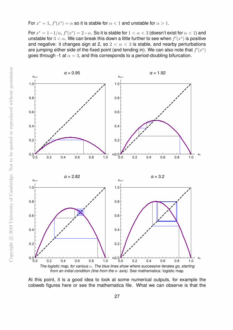
For x∗ = 1, f ′(x∗) = α so it is stable for α < 1 and unstable for α > 1.
For x∗ = 1−1/α, f ′(x∗) = 2−α. So it is stable for 1 < α < 3 (doesn’t exist for α < 1) andunstable for 3 < α. We can break this down a little further to see when f ′(x∗) is positiveand negative: it changes sign at 2, so 2 < α < 3 is stable, and nearby perturbationsare jumping either side of the fixed point (and tending in). We can also note that f ′(x∗)goes through -1 at α = 3, and this corresponds to a period-doubling bifurcation.
0.0 0.2 0.4 0.6 0.8 1.0��0.0
0.2
0.4
0.6
0.8
1.0
��+�α = ����
0.0 0.2 0.4 0.6 0.8 1.0��0.0
0.2
0.4
0.6
0.8
1.0
��+�α = ����
0.0 0.2 0.4 0.6 0.8 1.0��0.0
0.2
0.4
0.6
0.8
1.0
��+�α = ����
0.0 0.2 0.4 0.6 0.8 1.0��0.0
0.2
0.4
0.6
0.8
1.0
��+�α = ���
The logistic map, for various α. The blue lines show where successive iterates go, startingfrom an initial condition (line from the x- axis). See mathematica: logistic map.
At this point, it is a good idea to look at some numerical outputs, for example thecobweb figures here or see the mathematica file. What we can observe is that the
27

Cop
yri
ght
c ©20
19U
niv
ersi
tyof
Cam
bri
dge
.N
otto
be
quot
edor
repro
duce
dw
ithou
tp
erm
issi
on
behaviour is straightforward to α < 3. For 0 < α < 1 all trajectories head to the origin.For 1 < α < 2 all trajectories head into x∗ = 1−1/α from one side (which side dependson initial conditions). For 2 < α < 3, trajectories still head to x∗ but now in an oscillatoryway, resulting in the blocky spirals in the cobweb diagram11.
For α just a bit bigger than there, there looks to be a stable period-2 cycle, that is a pairof points where the map jumps from one to the other. Mathematically, x1 and x2 suchthat:
f(x1) = x2, f(x2) = x1 and x1 6= x2
Such x must satisfy f 2(x) = x, so we seek these solutions:
f 2(x)− x = 0
α f(x)(1− f(x))− x = 0
α2x(1− x) (1− αx(1− x))− x = 0
−α3x4 + 2α3x3 − α2(1 + α)x2 + (α2 − 1)x = 0
Then at this point it looks a hit hopeless, but there is actually a way forward: anysolution to f(x) = x will also be a solution to f 2(x) = x. So, we should be able tofactorise out f(x) − x, in fact exactly the expression we solved to find the fixed points.So working carefully, we can factorise out x[αx− α + 1]:
−x[αx− α + 1](α2x2 − α(α + 1)x+ (α + 1)
)= 0
We don’t want these fixed point solutions though (x1 6= x2 for a period-2 point), so cancancel these factors, leaving:
α2x2 − α(α + 1)x+ (α + 1) = 0 (10)
And hence:x1, x2 =
1
2α
((1 + α)±
√(1 + α)(α− 3)
)These can be assigned to x1 and x2 either way around. Looking at the square root,these exist for α > 3. When they appear at α = 3 they start at x = 2/3, i.e. where thefixed point is (x∗ = 1− 1/α).
Exercise 13: Check that f(x1) = x2 and f(x2) = x1
We can also check the stability of this period-2 cycle by considering f 2 (function appliedtwice) and checking if its derivative has modulus bigger than one or not, but there is a
11actually this must be why they are called ‘cobweb diagrams’, from the way oscillatory fixed pointslook like sort of like orb webs from spiders, but maybe only like that in minecraft.
28

Cop
yri
ght
c ©20
19U
niv
ersi
tyof
Cam
bri
dge
.N
otto
be
quot
edor
repro
duce
dw
ithou
tp
erm
issi
on
nice technique to make this simple in terms of algebra. Rather than going back to thebig expression for f 2(x), just use the chain rule:
d
dxf 2(x) =
d
dxf(f(x)) = f ′ (f(x)) f ′(x)
And at x1 (or x2), this gives is just f ′(x1)f ′(x2). We have that f ′(x) = α(1− 2x) so
f ′(x1)f ′(x2) = α(1− 2x1)α(1− 2x2) = α2[1− 2(x1 + x2) + 4x1x2]
and we can even read off the sum and product of x1 and x2 from the quadratic wesolved to find them (equation 10).
Exercise 14: Show that the period-2 cycle of the logistic map becomes unstableat α = 1 +
√6 ≈ 3.45
What happens for higher values of α? See Dynamical Systems course for more details,but in brief: there are a series of period-doubling bifurcations. We’ve found the first two,where the fixed point (a.k.a period-1) becomes unstable and a period-2 appears. Thenthe period-2 becomes unstable, and a period-4 will appear. This keeps going as α isincreased, but these all accumulate at a certain value (a∞ ≈ 3.5699). For α > α∞ thereare windows of ‘chaos’, but also windows where things settle to stable periodic orbits.
Bifurcation diagram, focusing on α > 3. For each value of α, this is made just by pickingrandom initial conditions for x and then iterating the map forward many times, throw thefirst few hundred iterates away, and then plot the results. Then keep doing this for lots of
values of alpha.end oflecture 5
29

Cop
yri
ght
c ©20
19U
niv
ersi
tyof
Cam
bri
dge
.N
otto
be
quot
edor
repro
duce
dw
ithou
tp
erm
issi
on
1.2.2 Higher order discrete systems
So far we have considered the case when the value of x in the next time step or gen-eration only depends on the current value. For many situations in biology, this is notenough: the dynamics may depend on earlier times also. We could develop some gen-eral theory, much like the box above but now for xn+1 = f(xn, xn−1, . . . , xn−p), but this isneither useful in practice nor informative. Instead we will explore a few examples, andsee techniques which can be applied more generally.
Example: discrete version of breathing
Recall the physiological example from earlier where breathing is regulated to adjust forvarying levels of carbon dioxide in the blood, with some lag. We can formulate a similarmodel in discrete time:
Vn+1︸︷︷︸Breath volume next step...
= f (Cn−k)︸ ︷︷ ︸... depends on CO2 k steps ago
= αCn−K
One could imagine a more general f , but here we just consider a linear example. Thenthe equation for carbon dioxide change in blood:
Cn+1 − Cn︸ ︷︷ ︸Change in CO2 in blood
= M︸︷︷︸CO2 added
− βVn+1︸ ︷︷ ︸breathed out
and as usual α, β and M are real, constant and positive. Note that this is actually notjust different from earlier breathing model by being discrete: the model for CO2 beingbreathed out is now just proportional to V and does not depend on C at all12. The stepsin n just represent some time step, e.g. minutes or breaths.
We can collapse this into a single variable:
Cn+1 = Cn +M − αβCn−k. (11)
Then seek constant solutions Cn = C∗:
C∗ = C∗ +M − αβC∗ =⇒ c∗ =M
αβ.
Now investigate stability of this steady state by perturbing13 as Cn = C∗ + δn and subin to (11):
C∗ + δn+1 = C∗ + δn +M − αβC∗︸ ︷︷ ︸=0
−αβδn−k
12Arguably, the earlier model is more sensible, where the higher the concentration in the blood, thehigher the amount of CO2 gets exchanged in lungs per volume of breath and expelled. This model isactually different, and chosen here just for convenient linearity later.
13not bothering with ε now, just think of δn as small
30
Cop
yri
ght
c ©20
19U
niv
ersi
tyof
Cam
bri
dge
.N
otto
be
quot
edor
repro
duce
dw
ithou
tp
erm
issi
on
δn+1 − δn + αβδn−k = 0
Normally we would then linearise in small δ, but this is already in right form here. Also,we could simplify slightly by making some compound parameter instead of αβ but thatis not essential.
Now we explore some different values of k. This is the time lag in steps between bloodlevels of CO2 taking a value and the breathing volume adjusting. First, for k = 0 wesimply have
δn+1 = (1− αβ)δn
and then it is clear that the steady state C∗ is stable for 0 < αβ < 2 and unstable forlarger αβ.
Next, try k = 1:δn+1 − δn + αβδn−1 = 0
To solve this linear difference equation, seek δn = pn solutions:
p2 − p+ αβ = 0 =⇒ p± =1
2±√
1
4− αβ.
and the general solution is a linear combination of these geometric solutions:
δn = Apn+ +Bpn−.
For 0 < αβ < 14, both p± are real and ∈ (0, 1), so pn decays for both, and hence C∗ is
stable.
For 14< αβ, both p± are complex14. This actually doesn’t change our approach very
much: we still need to know when solutions grow or decay and hence |p| < 1 orotherwise:
p± =1
2± i√αβ − 1
4=⇒ |p|2 =
(1
2
)2
+
(αβ − 1
4
)= αβ
hence for 14< αβ < 1 the steady state is stable (and a perturbation decays in an
oscillatory manner) and for 1 < αβ it is unstable. In summary, the steady state C∗is stable for 0 < αβ < 1 and unstable for larger values. As expected, the longer lagdecreases the range for stability (more parameter values are unstable).
This example worked out without too much difficulty as we could solve explicitly for p.This will be unlikely to work as we go up to higher order and therefore get somethingtrickier than a quadratic to solve. Sticking with k = 1, we can explore an alternativestrategy. For small αβ we could see that our roots for p all had modulus less than one,so all we need to do is to imagine turning up αβ until we the first time a root goes
14The p± are complex conjugates of each other. We will have real initial conditions for C and thereforeδ. This will make A and B complex conjugates and this will give real δn for all n.
31

Cop
yri
ght
c ©20
19U
niv
ersi
tyof
Cam
bri
dge
.N
otto
be
quot
edor
repro
duce
dw
ithou
tp
erm
issi
on
unstable. At the moment when this happens, a root will have modulus exactly one15.So, seek p = eiθ for some θ ∈ [0, 2π).
p2 − p+ αβ = 0 : e2iθ − eiθ + αβ
Then taking real and imaginary parts:
cos 2θ − cos θ + αβ = 0 (12)sin 2θ − sin θ = 0 (13)
Start with the simpler one, the imaginary part (13):
sin 2θ = sin θ =⇒ 2θ = θ + 2nπ or 2θ = (π − θ) + 2nπ
for n ∈ Z. Restricting attention to θ ∈ [0, 2π):
θ = 0 orπ
3,3π
3,5π
3
The real part will supply the corresponding values of αβ:
αβ = 0 or 1,−2, 1
And as we are looking for the first positive16 αβ, we see this is αβ = 1. This correspondsto θ = π/3 or θ = 5π/3. Equivalently, this is
p± = e±iπ3 =
1
2± i√
3
2
which matches up with our first approach. Note that p6 = 1 for both p+ and p−, so smallperturbations satisfy:
δn+6 = Apn+6+ +Bpn+6
− = Apn+ +Bpn− = δn
so have period 6 at the boundary (at least to linear order), and close to period 6 justabove and below.
0 10 20 30 40 50�
��
αβ = ����
0 10 20 30 40 50�
��
αβ = �
0 10 20 30 40 50�
��
αβ = ����
Typical solutions for k = 1 for various αβ near to threshold for stability, starting from aperturbation away from steady state.
15Actually expect this to happen in complex conjugate pairs. We are implicitly assuming that rootsare continuous in our model parameters (which does not seem too unreasonable in math bio). We arealso assuming that the offending root(s) actually goes right through modulus one: technically it wouldbe possible to just reach modulus one and then go back inside the unit circle. That would just be mean.
16actually the solution at zero corresponds to a root p = 1 exactly at αβ = 0, and this root edges justbelow one as we make αβ small but positive. So this is moving into the region for stability, not movingout!
32

Cop
yri
ght
c ©20
19U
niv
ersi
tyof
Cam
bri
dge
.N
otto
be
quot
edor
repro
duce
dw
ithou
tp
erm
issi
on
Example: Multi-generation model
Another set of problems which leads to higher order discrete systems is when the timesteps are population generations and multiple generations need to be considered tofind the next generation size. For example, a type of annual plant produces γ seedsin the summer and then dies. Those seeds stay in the ground over the winter. Thenext summer, each seed17 has probability σ of successfully germinating and growinginto a new adult plant. Failing that, the seed will germinate the summer after that withprobability τ . Assume they cannot germinate after that.
We turn this wordy description into equations18, accounting for number of adult plantsat season n by xn, seeds that have been waiting one year as s(1)
n and two years as s(2)n .
Then
xn = σs(1)n + τs(2)
n
s(1)n = γxn−1
s(2)n = (1− σ)s
(1)n−1
Then we can go from this system in multiple variables to one in a single variable, andhere the only sensible choice is xn:
xn = σγxn−1 + τ(1− σ)γxn−2. (14)
Indeed, arguably it would be possible to go straight here from the description in words.Note γ > 0 and σ, τ ∈ [0, 1] as they are proportions.
Note that equation (14) is linear in x and the steady state solution is x∗ = 0. In theorywe now propose a perturbation, sub it in, linearise, but of course in this case we justget the same equation back again. So, directly go for xn = pn:
p2 − σγp− τ(1− σ) = 0
17Think of this as proportion of seeds, as there are lots of seeds lots of seeds18Indeed, this is half of the art of math bio in practice in research, except the wordy descriptions tend
to be a lot more vague on crucial details and then there’s a lot of decisions for the modeller to make.
33

Cop
yri
ght
c ©20
19U
niv
ersi
tyof
Cam
bri
dge
.N
otto
be
quot
edor
repro
duce
dw
ithou
tp
erm
issi
on
p± =σγ
2± 1
2
√σ2γ2 + 4γτ(1− σ)
As the contents of the square root is positive, these roots are real. We can also seethat the roots are positive and negative with the positive root having the larger modulus(i.e. 0 < −p− < p+). Solutions will be of the form
xn = A1pn+ + A2p
n−
and the first term will dominate as n increases. In fact, we just need to check p+ forstability19.
Seeking p+ = 1 and a little algebra we arrive at
γ [σ + (1− σ)τ ] = 1
It is worth stepping back into original meaning of the parameters at this point. Consid-ering this, the square bracket is the proportion of seeds that ever germinate, and theprefactor γ is the number of seeds produced by each adult plant ever. So γ[..] is themean number of offspring per plant. Call the whole thing K:
K = γ [σ + (1− σ)τ ]
It is not surprising that it determines the boundary for stability:
mean offspring = K < 1, x = 0 is stable
mean offspring = K > 1, x = 0 is unstable
It is often the case that conditions on the boundary for stability has an intuitive expla-nation in terms of the original biological model. It is worth looking out for these as theyare a good check that the algebra has come out correctly and the answer is sensible. end of
lecture 6
19If it is greater than one, then xn grows eventually regardless of p−. If it is less than one, then p− alsohas modulus less than one, so xn decays towards zero eventually.
34

Cop
yri
ght
c ©20
19U
niv
ersi
tyof
Cam
bri
dge
.N
otto
be
quot
edor
repro
duce
dw
ithou
tp
erm
issi
on
1.3 Multi-species models
The dynamics of interacting populations (or biological substances) gives rise to themost interesting models in mathematical biology. In the next few sections, we will workthrough a series of examples, illustrating more general principles and techniques.
1.3.0 Revision: 2-D stability in continuous time
Consider the system:
du
dt= f(u, v)
dv
dt= g(u, v)
A fixed point (u∗, v∗) satisfies f(u∗, v∗) = 0 and g(u∗, v∗) = 0.
To explore stability, consider a small perturbation to that fixed point. Set u(t) = u∗+ξ(t),v(t) = v∗ + η(t) and expand in small ξ, η:
dξ
dt= f (u∗ + ξ, v∗ + η) = f(u∗, v∗)︸ ︷︷ ︸
=0 at FP
+ ξ∂f
∂u
∣∣∣∣FP
+ η∂f
∂v
∣∣∣∣FP
+O(ξ2, ξη, η2)
Similarly:dη
dt= g (u∗ + ξ, v∗ + η) = ξ
∂g
∂u
∣∣∣∣FP
+ η∂g
∂v
∣∣∣∣FP
+O(ξ2, ξη, η2)
So the local dynamics comes down to the Jacobian:(ξ
η
)=
(∂f∂u
∂f∂v
∂g∂u
∂g∂v
)∣∣∣∣∣FP
(ξ
η
)where the 2×2 matrix is the Jacobian. In practice, just find the Jacobian and start fromthere. We might sometimes want the eigenvectors to help draw phase-diagrams, butusually we just want the eigenvalues.
Or even more basic, we just need to know the sign of the real parts of the eigenvalues.Let T be the trace and D the determinant of the Jacobian evaluated at some fixedpoint. Then (for 2-D), the eigenvalues are:
λ = −1
2T ± 1
2
√T 2 − 4D
or alternatively the other way T = λ1 + λ2 and D = λ1λ2. So
D < 0 : saddle
D > 0, T < 0 : stable
D > 0, T = 0 : centre
D > 0, T > 0 : unstable
35

Cop
yri
ght
c ©20
19U
niv
ersi
tyof
Cam
bri
dge
.N
otto
be
quot
edor
repro
duce
dw
ithou
tp
erm
issi
on
We could then subdivide the stable and unstable cases according to focus or node(eigenvalues complex or real) by checking T 2 − 4D, but often in math bio we do notneed to do this.
1.3.1 Competition models
The classic example is
N1 = r1N1
(1− N1
K1
− b12N2
K2
)N2 = r2N2
(1− N2
K2
− b21N1
K1
).
where there are two species N1 and N2. Each species alone has simple logistic dy-namics (see lecture 1) with linear growth, and a negative quadratic term which meanseach species has some stable equilibrium size (K1 and K2 respectively: the carryingcapacities for each species alone). The terms with the b12 and b21 are the interactionsbetween the species: they each slightly ‘harm’ the other. An analysis of this system isone of the questions on examples sheet 1. The net outcome is not too surprising: ifthe negative interaction terms are not too big, then the two species will coexist at somestable equilibrium value. If the interaction terms are too strong, then the two speciescannot stably coexist, and one or other species wins out.
Here we study instead a different competition system, motivated by recent research oncontrolling the spread of dengue. Dengue is a virus that causes disease in humans.Rather than being transmitted directly from human to human, it requires and interme-diate vector: a mosquito. If the mosquito bites and takes blood from someone who isinfected, the mosquito could go on to infect anyone they bite later.
You can read a lot more about the ideas on the Eliminate Dengue website20, but inbrief: Wolbachia are a type of bacteria that can infect a huge range of insect species.Researchers have developed a strain of Wolbachia that can infect the kind of mosquitosthat can carry dengue. The bacteria seems to block transmission of dengue virus, sowe would like to see if this would be a viable way to control dengue in practice. Recentresearch suggests that the same approach will work for Zika virus, but there is morework to be done on this. For whichever virus, our question is the same: if we introducesome mosquitos that carry Wolbachia into the wild, will eventually all mosquitos carryWolbachia?
In mosquitos, Wolbachia is only transmitted vertically, which means to offspring mosquitos(as opposed to ‘horizontal transmission’: to general others in same species). If a fe-male mosquito is infected, her eggs will certainly be infected, regardless of the carrierstatus of the male. She will also produce fewer eggs than usual. Here’s the weird bit:
20http://www.eliminatedengue.com/
36

Cop
yri
ght
c ©20
19U
niv
ersi
tyof
Cam
bri
dge
.N
otto
be
quot
edor
repro
duce
dw
ithou
tp
erm
issi
on
if the female is uninfected but the male is infected, the eggs will not be viable at all, sono offspring at all. Now we start pulling this into a mathematical formulation.
Let x be the number of uninfected female mosquitos, and y be the number of infectedfemale mosquitos. Assume that the uninfected mosquitos have a per capita death rated and a bonus per capita death rate of ε times the total number of female mosquitos(competition). The infected mosquitos have shorter lifespans on average, which wemodel here as a higher death rates by having an additional factor µ with d (µ > 1).
We do not need to explicitly track the males: just assume their infection state is in pro-portion to the females (which you can check is the case by building full equations if youreally want), so a proportion x/(x+y) uninfected. Also assume there are enough malesaround for all eggs to be fertilised. Suppose that in a purely uninfected population, therate of viable eggs for female mosquitos being produced is r per female capita. If thefemale is infected, assume that they produce λ times the normal number of eggs, soλ < 1.
Summarising the four possible crosses (female-male infection status combinations):
Cross Frequency Egg rate State
F × M x. xx+y
r Uninfected
F × M x. yx+y
0 @
F × M y. xx+y
λr Infected
F × M y. yx+y
λr Infected
Where the F means infected and F is uninfected females, similarly for M and M formales.
Bringing this together, we get the following system:
x = r xx
x+ y− d x− ε x(x+ y)
y = λr yx
x+ y+ λr y
y
x+ y− µd y − ε y(x+ y)
By rescaling time by a factor r and both x and y by a factor ε/r, the system can beslightly tidied21:
x = x
[x
x+ y− d
r− (x+ y)
]y = y
[λ − µd
r− (x+ y)
]21There’s a wording ambiguity about which direction is meant by ‘rescale by a factor’, but interpret
here in the direction that tidies things up!
37

Cop
yri
ght
c ©20
19U
niv
ersi
tyof
Cam
bri
dge
.N
otto
be
quot
edor
repro
duce
dw
ithou
tp
erm
issi
on
Looking at each population alone (i.e. forcibly setting x = 0 or y = 0), each is justlogistic, and we can pick out the equilibrium single population sizes:
Uninfected only, y = 0 : x = x
(1− d
r− x)
= x (x0 − x)
Infected only,x = 0 : y = y
(λ− µd
r− y)
= y (y0 − y)
where x0 = 1 − d/r and y0 = λ − µd/r are the equilibrium sizes of each populationalone.
Now take some sensible assumptions, thinking about the case that we wish to model.We are imagining an uninfected resident population, so they are viable, i.e. r > d sox0 > 0. We also want to consider the case when the purely infected population isviable, otherwise the proposed introduction is hopeless anyway, so assume λr > µd,i.e. y0 > 0. We have already assumed that infection reduces the number of eggs (λ < 1)and infection increases the death rate (µ > 1). So putting all these together, we have0 < y0 < x0 < 1.
This has demonstrated another strategy for rescaling parameters: discover a meaning-ful parameter combination by considering the relatively simple equilibrium points suchas each population alone, then see if the system can be written out nicely in terms ofthese quantities. It works well for this example. Organising the parameters to be interms of x0 and y0, the full system becomes:
x = x
[x0 −
y
x+ y− (x+ y)
]y = y
[y0 − (x+ y)
]
There are four non-negative fixed points: no mosquitos (0, 0), purely uninfected (x0, 0)or purely infected (0, y0), and an interested mixed state one (x1, y1), where setting thesquare brackets to zero and working through:
x1 = y0(1− x0 + y0) and y1 = y0(x0 − y0)
and as 0 < y0 < x0 < 1, both x1 and y1 are positive.
Exercise 15: Check the Jacobian at (x1, y1) and show that it corresponds to asaddle
The next stage is to find the null clines and then put together the phase diagram.Nullclines are just when x = 0 and when y = 0. On these, the trajectories are pure
38

Cop
yri
ght
c ©20
19U
niv
ersi
tyof
Cam
bri
dge
.N
otto
be
quot
edor
repro
duce
dw
ithou
tp
erm
issi
on
vertical and pure horizontal respectively. But more usefully, these curves also divideup the phase plane into regions where the direction of trajectories is purely in onequadrant (e.g. up and left), which helps pulling the picture together.
x = 0 :
x = 0 or y = x0(x+ y)− (x+ y)2
y = 0 : y = 0 or x+ y = y0
Finally, we may answer our original question: what happens if we start at the uninfectedequilibrium and introduce some infected mosquitos? This is sketched below: it reallydepends where the dividing line is between basins of attraction of the two stable fixedpoints. The dividing line (separatrix) goes through the saddle point (indeed it is thestable manifold of the saddle point).
A schematic of the different outcomes of an introduction of infected mosquitos. Theshaded area in each case is the region where trajectories would head towards (x0, 0),
drawn for two different examples. The red dot is where we are on the phase diagram afteran introduction of a certain number of infected mosquitos. Clearly, if we want all
mosquitos infected eventually, we would like to be in the righthand regime.
So introducing a very small number of mosquitos is not enough, there has to be quitea few infected mosquitos brought in. However, on the plus side, once the infected
39

Cop
yri
ght
c ©20
19U
niv
ersi
tyof
Cam
bri
dge
.N
otto
be
quot
edor
repro
duce
dw
ithou
tp
erm
issi
on
population is established, it won’t easily revert back.
Exercise 16: Imagine you are a mathematical modeller advising on this project.The experimentalists can work to change the strain of Wolbachia so as to makeit less damaging to the mosquitos by softening the effect on the death rate(decrease µ towards 0) or the egg production rate (increase λ towards 1). Wewould like to make it so that a small introduction of infected mosquitos would beenough to make all mosquitos infected eventually. Would you advise them toconcentrate their efforts on λ or µ or a combination of the two? (Hint: considerthe impact on x0 and y0 and then the nullclines).
We come back to this example later in the course, when we consider the spatial effects.end oflecture 7
1.3.2 Predator-prey models
No course in math bio would be complete without this iconic system: the Lotka-Volterramodel of predator-prey dynamics. The prey population (size N ) would grow on itsown, and the predator population (size P ) would decay on its own. The interactionis predation which happens at rate proportion to the product of both population sizes:mass-action. The predation harms the prey and benefits the predators. This leads tothe system
dN
dt= aN − bNP = N(a− bP )
dP
dt= cNP − dP = P (cN − d)
where a, b, c and d are all positive. This can be rescaled to
u = u (1− v)
v = −α v (1− u)
Exercise 17: Carry out this rescaling and show that α = d/a (and also noteα > 0).
There are two fixed points: (0, 0) and (1, 1). The general Jacobian is given by
J =
(1− v −uαv −α(1− u)
)
40

Cop
yri
ght
c ©20
19U
niv
ersi
tyof
Cam
bri
dge
.N
otto
be
quot
edor
repro
duce
dw
ithou
tp
erm
issi
on
So evaluating at the fixed point at the origin:
J(0,0) =
(1 00 −α
)And checking the eigenvalues22 we see that the origin is a saddle. This is not a surpriseas we geared the model so the prey would group on their own and the predators woulddecay.
The non-trivial fixed point gives
J(1,1) =
(0 −1α 0
)T = 0, D = α λ = ±i
√α
which corresponds to a centre. This is neither stable nor unstable to linear order, andin theory requires further work to determine non-linear stability (higher-order terms).
Nullclines In sketching phase diagrams, fixed point analysis gives us the dynamicsclose to equilibrium values, and we are left to join up the picture in between. Very often,it is useful to divide up space into regions where u and v are positive or negative. Thismeans finding the nullclines: curves where one or other variable is unchanging.
For the Lotka-Volterra system:
u = 0 : u = 0 or v = 1
v = 0 : v = 0 or u = 1
This is starting to suggest that trajectories might be cycles: closed curves so the solu-tion is periodic. However neither the Jacobian nor the diagram with the nullclines hasconclusively shown that we have cycles. Luckily, we can explicitly find the trajectoriesfor this system. Start by removing the time dependence to just think about curves in u,v space:
du
dv=u
v=−u(1− v)
αv(1− u)
22The matrix is diagonal, so just read off the eigenvalues
41
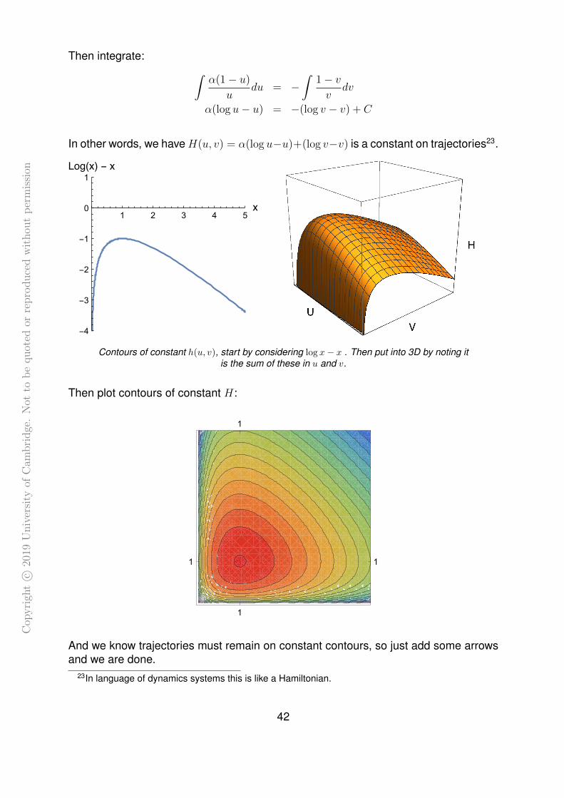
Cop
yri
ght
c ©20
19U
niv
ersi
tyof
Cam
bri
dge
.N
otto
be
quot
edor
repro
duce
dw
ithou
tp
erm
issi
on
Then integrate: ∫α(1− u)
udu = −
∫1− vv
dv
α(log u− u) = −(log v − v) + C
In other words, we haveH(u, v) = α(log u−u)+(log v−v) is a constant on trajectories23.
1 2 3 4 5�
-4
-3
-2
-1
0
1���(�) - �
Contours of constant h(u, v), start by considering log x− x . Then put into 3D by noting itis the sum of these in u and v.
Then plot contours of constant H:
1
1
1
1
And we know trajectories must remain on constant contours, so just add some arrowsand we are done.
23In language of dynamics systems this is like a Hamiltonian.
42

Cop
yri
ght
c ©20
19U
niv
ersi
tyof
Cam
bri
dge
.N
otto
be
quot
edor
repro
duce
dw
ithou
tp
erm
issi
on
For the Lotka-Volterra system, we can also show that the time-average of the periodorbits are all equal to the values of the population size at the fixed point. These wereboth normalised to 1 here, but it still holds for the system before rescaling of course.Starting from u = u (1− v) and integrating over one period:
∫1
udu =
∫1− v dt
[log u]︸ ︷︷ ︸=0 as same u at each end
=
∫1 dt︸ ︷︷ ︸
period T
−∫v dt︸ ︷︷ ︸
T× average v
So the time-average value of v is 1. A similar calculation starting from v shows that thetime-average of u is also 1. This is true no matter which contour of H we are on.
1�
1
�
�
�
�
1
�
�
�
1
�
�
�1
Solutions of the Lotka-Volterra system for assorted starting conditions, with thetrajectories shown also together in the u, v plane. Note that the vertical scale changesbetween plots, but the dotted line marks 1, the time-average of both populations. It can
also be seen from these solutions that the prey (blue) lead and the predators (red) follow.
The effect of fishing Returning to the unscaled original system, we can ask thequestion: what is the effect of fishing on the system? We simulate this by introduc-ing terms representing fishing of both populations at a constant per capita rate (butpotentially different constants for predators and prey):
43

Cop
yri
ght
c ©20
19U
niv
ersi
tyof
Cam
bri
dge
.N
otto
be
quot
edor
repro
duce
dw
ithou
tp
erm
issi
on
N = N(a− bP )− fNN = N ((a− fN)− bP )
P = P (cN − d)− fPP = P (cN − (d+ fP ))
And this is just the same system as before with just a tweak of parameters: a is replacedby a − fN and d is replaced by d + fP (taking care with the signs). So now no furtherserious work is needed: just look at the effect of shifting the parameters. The fixedpoint moves:
Originally at
(d
c,a
b
)Now:
(d+ fPc
,a− fNb
)i.e. a higher number of prey and lower number of predators. We also know from abovethat the time-average of the cycles will similarly move.
������� ������
���� ������
��
�+���
�
��
�-���
�
This result is remarkably simple, but maybe slightly surprising: fishing is depleting bothpopulations, yet the net result is actually an increase in the prey population. The ef-fects of fishing are concentrated in the predators. In general, when we have multiplepopulations in balance with each other and their environment (an ecosystem) externalinterventions can have non-obvious effects. Mathematical models can help us under-stand these24. Vito Volterra used exactly the system we have studied here to under-stand the changes in fish population in the Adriatic. During war time, fishing was lowerthan usual but the proportion of the catch that were predators (sharks etc.) went up.This is rather elegantly explained by the above analysis.
The cycles are not robust! That we have cycles is pretty special. If we change thestructure of the Lotka-Volterra system in almost any way25 then the cycles will break.Here we look at the example of adding logistic-style quadratic terms, which represent
24This is where mathematical biology has been historically most successful: at explaining observedphenomena.
25The parameter tweak of fishing was not a structural change.
44

Cop
yri
ght
c ©20
19U
niv
ersi
tyof
Cam
bri
dge
.N
otto
be
quot
edor
repro
duce
dw
ithou
tp
erm
issi
on
interaction within each species alone: intra-specific competition adds to the death rate.Working now in the rescaled system:
u = u (1− v)− εuu2
v = −α v (1− u)− α εvv2
Assume both rates εu, εv � 1 so the change to the system is small26. Note the factorof α in new term in the second equation: this is just to make the algebra tidier, as thesystem can now be written:
u = u [1− v − εuu]
v = −α v [1− u+ εvv]
Look for fixed points, paying attention only to u ≥ 0 and v ≥ 0.
Exercise 18: Show that there are three fixed points now.
• The usual trivial fixed point (0, 0)
• Prey population only (at their logistic equilibrium): (ε−1u , 0)
• One with both populations present: (u∗, v∗) where
u∗ =1 + εv
1 + εuεvand v∗ =
1− εu1 + εuεv
and hence u∗ > 1, v∗ < 1.
Use the Jacobian27 to analyse the stability of this fixed point.
J(u∗,v∗) =
[1− v∗ − εuu∗]︸ ︷︷ ︸
=0
+u∗(−εu) −u∗
αv∗ −α [1− u∗ + εvv∗]︸ ︷︷ ︸=0
−αv∗εv
=
(−εu u∗ −u∗αv∗ −α v∗ εv
)=
(− −+ −
)And hence T < 0 and D > 0 and this is always a stable fixed point.
26Or at least it is small for sensible u, v, i.e. on scale of original fixed point27Three useful tricks: (i) keep brackets intact as long as possible: for example in finding the fixed
point you will have solved (1 − v − εuu) = 0 so keep it together when differentiating and then it will beeffortlessly zero at the fixed point; (ii) don’t sub in the espressions for u∗ and v∗ too soon, just keep themas u∗ and v∗ as long as possible; (iii) often we don’t even need the full Jacobian evaluated: it is enoughto see the signs of the entries, sometimes.
45

Cop
yri
ght
c ©20
19U
niv
ersi
tyof
Cam
bri
dge
.N
otto
be
quot
edor
repro
duce
dw
ithou
tp
erm
issi
on
Exercise 19: Continue this example by using nullclines.
Hint: think about the competition terms and how their main effect is to ‘push’large u and v inwards.
Exercise 20: For those who did dynamical systemsa: construct a (strict)Lyapunov function to show (u∗, v∗) attracts all trajectories that start in u, v > 0.
Hint: H(u, v) was constant before, so seems like a good place to start.
afor those that didn’t but are unlikely to be put off by my warnings: good for you! All youneed here is that a Lyapunov function V (u, v) is such that it is strictly decreasing along trajec-tories in this domain, except at the fixed point (where is is constant). The function V should becontinuous and zero at the fixed point, positive everywhere else. If you find such a function, tra-jectories have V decreasing and bounded below, so V tends to some constant, so trajectoriestend to a some set where V = 0, which here is just the fixed point.
end oflecture 8
1.3.3 Chemical kinetic models
The big yellow blob is the bacterium, the blue things are the receptors and the pink dotsare the nutrients. OK so a bit of imagination required!
Imagine a single bacterium. It has receptors ready to pick up nutrients. The receptorsstart empty (E) and pick up nutrients in a substrate (S). Receptors then carry the nu-trient so there is a complex (C) consisting of a reception and a nutrient particle. Thisgoes into the bacterium where the nutrient is dropped off to be final product (P). Wecan describe this in terms of chemical kinetic notation as follows:
E + Sk1−−−−−⇀↽−−−−−k2
C
Ck3−−−−−→ E + P
46

Cop
yri
ght
c ©20
19U
niv
ersi
tyof
Cam
bri
dge
.N
otto
be
quot
edor
repro
duce
dw
ithou
tp
erm
issi
on
with three rates: k1 is the rate that E and S combine, k2 is the rate at which C can failand fall apart back into E and S, and k3 is the rate at which C is internalised and dropsoff P and becomes an empty E again.
To set up differential equations, suppose that everything is large numbers so that wecan sensibly talk about concentrations. Let s be the concentration of S, and similarlyfor e, p and c. Then in differential equations, our system can be described as
s = −k1 e s+ k2 c
e = −k1 e s+ k2 c+ k3 c
c = +k1 e s− k2 c− k3 c
p = + k3 c
For initial conditions, suppose that we start with all the nutrients outside and all recep-tors empty, so s(0) = s0, e(0) = e0, c(0) = 0 and p(0) = 0, for some s0, e0 > 0. Alsosuppose that there are a lot more nutrients than receptors, so that receptors are usedmany times before the substrate is fully depleted: s0 � e0.
From thinking about the original scenario, we can immediately see that there must besome invariant quantities. In particular, the number of receptors stays constant if weinclude both carrying (C) and empty (E). Also the nutrients are constant if we considerthem outside (S), being carried (C) and inside (P).
We could also see this from the equations by spotting combinations that add to give nochange:
e+ c = 0 , s+ c+ p = 0
so these are constant, and we can determine the constants by initial conditions:
e+ c = e0 , s+ c+ p = s0 .
We can use these to go from four differential equations down to two, substituting fore and p (in principle at least, p doesn’t actually occur anywhere). This is our reducedsystem:
s = −k1(e0 − c)s+ k2 c = −k1 e0 s+ (k1 s+ k2)c
c = +k1(e0 − c)s− k2 c− k3 c = +k1 e0 s− (k1 s+ k2 + k3)c
This is already much better, but we can rescale further by strategic use of our initialconditions. We set u = s/s0 and v = c/e0 and then these have nice interpretations: u isthe proportion of total nutrient still available (so u is one initially) and v is the proportionof receptors that are currently carrying nutrient (so v is zero initially). We could alsorescale time to adsorb one of the rates.
47

Cop
yri
ght
c ©20
19U
niv
ersi
tyof
Cam
bri
dge
.N
otto
be
quot
edor
repro
duce
dw
ithou
tp
erm
issi
on
Exercise 21: By a suitable rescaling, turn the system into:
u′ = −u+ (u+ µ− λ)v u(0) = 1
εv′ = +u− (u+ µ)v v(0) = 0
whereλ =
k3
k1 s0
, µ =k2 + k3
k1 s0
, ε =e0
s0
� 1 .
We see that the v dynamics are faster than the u dynamics (by an order of 1/ε). Sowe can see what the solutions will be like without doing too much more work. Do the vdynamics first imagining u to be almost fixed. We can see that it is exponential decaydown to a constant:
v =u
u+ µ
where the decay is fast (takes order ε time). So assume that has happened, and as wenow slowly change u, the fast dynamics of v ensures it keeps moving quickly back toits equilibrium value again (which is itself a function of u). Substitute this value of v intothe u′ equation:
u′ = −u+ (u+ µ− λ)u
u+ µ= − λu
u+ µ
so we can see that u just decays towards u = 0.
1�
1/2
1�
This is for ε = 0.1 which is not super small, and even then it is clear the trajectories quicklymove to v = u/(u+ µ). The red trajectory is for the initial condition u = 1, v = 0.
48

Cop
yri
ght
c ©20
19U
niv
ersi
tyof
Cam
bri
dge
.N
otto
be
quot
edor
repro
duce
dw
ithou
tp
erm
issi
on
1�
1/2
1�
Same but for ε = 0.01, when the fast-slow dynamic is clearer: trajectories move verticallyfirst until they are near the v = u/(u+ µ) curve, then they move slowly along that curve
Thinking back to the original system, the v dynamics being fast just means that the pro-portion of receptors occupied quickly settles to some value and then slowly readjustsas the nutrient is depleted. This was all a consequence of our original assumption ofthere being much more nutrient out there than the total number of receptors.
This system is actually a classic model for enzyme kinetics used by biochemists (Michaelis-Menten).
Exercise 22: Work back to the original system and show that the inverse of therate of nutrient uptake is linear in the inverse of substrate. In other words:(
dp
dt
)−1
= A+B s−1
for some constants A and B.
In principle this gives a test for whether a set of observations are consistentwith Michaelis-Menten kinetics. In practice, one should probably be more thanmildly concerned about issues with inverting small numbers, when those smallnumbers are hard-to-measure experimental quantities.
49

Cop
yri
ght
c ©20
19U
niv
ersi
tyof
Cam
bri
dge
.N
otto
be
quot
edor
repro
duce
dw
ithou
tp
erm
issi
on
Exercise 23: Translate this to differential equations:
2 C + X0k1−−−−−⇀↽−−−−−µ1
X1λ1−−−−−→ X0 + P
2 C + X1k2−−−−−⇀↽−−−−−µ2
X2λ2−−−−−→ X1 + P
Also, find an invariant sum. You can do this by considering the reactions abovedirectly, or by inspecting your differential equations (I think it is usually easierto spot these from the reactions directly.)
Note that 2 C is shorthand for C + C, so reaction rates will involve c2. Similarly3C and so on.
1.3.4 Epidemic models
There is a long and fruitful tradition of using mathematical models to capture how in-fectious disease spreads through a population. The most classic model (first publishedover a century ago) is so-called ‘SIR’ model. Here, the population is divided into threegroups: susceptible (S), infected/infectious (I) and recovered/removed (R). This com-partmental model is a little different to the population models we have seen already. Inpredator-prey and competition models that we have considered so far, the groups arereally separate and it is not possible to move from one to another: you’re there frombirth to death. Here, it is possible to move between S, I and R. This type of model isusually called a ‘compartmental model’ where there are flows and interaction betweencompartments. It works for populations as well as chemical kinetics (see below) amongmany other things.
Here we have two processes causing a flow between compartments: infection takesindividuals from S to I and recovery takes them from I to R. For now, we do notinclude any births or deaths: we are thinking of some short outbreak of disease in aclosed population. The full system is:
S = −βISI = +βIS − νIR = + νI
The total rate of infection is mass-action: proportional to the product of S and I. Wehave seen interaction terms like this before, for example in predation (N × P ). It cor-responds to the frequency of the two groups encountering each other. Or another wayto think about it is that the rate per capita of infection is proportional to the number ofinfected I, the number available to infect is S, so the total rate is proportional to S × I.We call coefficient β the transmission rate. The recovery term is simpler, just simplerate per individual: ν.
50

Cop
yri
ght
c ©20
19U
niv
ersi
tyof
Cam
bri
dge
.N
otto
be
quot
edor
repro
duce
dw
ithou
tp
erm
issi
on
It is easy to see that the total population size remains constant here28. We then denotetotal population size as N = S+ I +R, and see N = 0. So if we know N (think of as anextra parameter), then knowing any two of S, I and R is enough to determine the third.So, we might as well drop R from the system, and actually we don’t even need to subR = N − I − S in anywhere as it does not occur in the other equations:
S = −βISI = +βIS − νI
We can reconstruct R if we even need it, which we rarely do in practice. Usually I ismost visible, perhaps followed by S.
We can solve for S and I numerically without much difficulty, and here is a typical outputwhen we start with a few infecteds and the rest susceptible:
�
�
�
����
� �� �
When can an epidemic happen?
An ‘epidemic’ is simply when the cases increase, i.e. I > 0. So initially t = 0 and
I(0) = [βS(0)− ν]I(0)
and assume that one or a few infected are introduced initially so that I(0) > 0. Thewe just need to check the sign of [βS(0) − ν] (where S(0) is just the initial number ofsusceptibles). Imagine that we are starting from nearly everyone susceptible, and onlya very small number infected, then S(0) ≈ N . We see that an epidemic is possible ifand only if
β
νN > 1 .
28Disturbingly, this all still works for fatal diseases: the R compartment serves equally well for thosewho have recovered and are now fit and well and now immune to the disease, as those who are in factdead. Either way, they can’t get the disease again. We just call them all ‘removed’, which always seemsa bit uncaring.
51

Cop
yri
ght
c ©20
19U
niv
ersi
tyof
Cam
bri
dge
.N
otto
be
quot
edor
repro
duce
dw
ithou
tp
erm
issi
on
As always, we should try and interpret this inequality. Looking at the lefthand side,the trickiest bit is the 1/ν. We know ν is the recovery rate per individual. One way toimagine this is as a random process with event happening at rate ν if it hasn’t happenedalready. This leads to an exponential distribution of time to recovery. The expected timeto recovery is 1/ν, i.e. the duration of a infection. This is multiplied by β, which is therate that one individual infects each susceptible29. Finally, N is roughly the numberof susceptible individuals around. So, time infected, rate of on infected infecting eachcontact, number of contacts: the product is total number infected, on average, fromone infection.
Actually this idea holds more generally in disease modelling, and this number is knownas the reproductive ratio, or R0
30. Note this is an unfortunate piece of historical notationas this R0 has nothing to do with the R of SIR. It is defined as the mean number ofsecondary cases in an otherwise susceptible population. In other words, if we dropone infected into our susceptible population, how many others will they directly infect?For this classic SIR model, we have found:
R0 =β
νN .
and our threshold for an epidemic is R0 > 1. This of course is also the threshold inmore general models also, once we have identified R0 (which is not always easy to doin practice31). end of
lecture 9
Vaccination We actually have enough to say quite a bit about the potential for va-cation as a control measure, without going into the differential equations in any furtherdetail. Suppose that we intervene before a possible epidemic to vaccinate a proportionp of the population, and assume the vaccine gives total protection against the disease.This is equivalent32 to moving a proportion p of the population straight into R and leav-ing S(0) ≈ (1− p)N . Our condition for an epidemic to be possible is now
β
νS(0) =
β
ν(1− p)N = (1− p)R0 > 1 .
We can rearrange this to find the threshold for p in terms of R0: p < 1 − 1/R0 for anepidemic to be possible:
29a sort of per capita per capita30pronounced R-nought31There’s plenty more to read and learn about R0, and this paper by Heffernan et al. is a good place
to start: http://doi.org/10.1098/rsif.2005.004232All of this is for a perfect vaccine, so being vaccinated means you truly in R. One can easily extend
this to think about imperfect vaccines.
52

Cop
yri
ght
c ©20
19U
niv
ersi
tyof
Cam
bri
dge
.N
otto
be
quot
edor
repro
duce
dw
ithou
tp
erm
issi
on
����������
��������������
���������� �������������
�������� �������������
� � � � � � � � � � �������
���
���
���
���
����
If R0 is less than one, there’s no chance of an epidemic anyway, so no need to vacci-nate. For R0 > 1, there is some pc ∈ (0, 1) which is the vaccination threshold. It is nottoo hard to understand this intuitively, and to see why it depends on R0 only. We’d liketo vaccinate enough individuals so that the disease cannot spread through the popula-tion. We’d like to make the effective reproduction ratio less than 1. If we introduce oneinfected and they would infect R0 others, we’d like to vaccinate at least R0 − 1 of thoseR0. That’s just the proportion pc.
This is all interlinked with the idea of herd immunity which is the idea that having manyindividuals immune can even protect other individuals. For each person vaccinated, itprotects not just that person, but all the people they would have gone on to infect, andeven later generations of infection onwards. These ideas are not new to mathemati-cians, and can be thought about more generally in terms of percolation theory.
Epidemic and final size
We can go further with this simple model and learn something of the trajectory of anepidemic once it does start. Here, it does not make sense to do a traditional fixed pointanalysis: the whole the epidemic is itself transient behaviour.
At the end of an epidemic, the susceptibles are not fully depleted: S seems to plateauto some positive value. Actually, we can understand this by considering the S − Iphase-plane. The whole of I = 0 is a line of fixed points, but it is not so much these weare interested in as the trajectories that arrive at them. We can explicitly solve for I asa function of S in this case:
dI
dS=I
S=
+βIS − νI−βIS
= −1ν
βS= −1 +
N
R0
1
S
And integrating with respect to S:
I = −S +N
R0
logS + C
53

Cop
yri
ght
c ©20
19U
niv
ersi
tyof
Cam
bri
dge
.N
otto
be
quot
edor
repro
duce
dw
ithou
tp
erm
issi
on
for some constant C which is determined by initial conditions (now thinking about I andS as functions of time again):
[I(t)− I(0)] = − [S(t)− S(0)] +N
R0
log
[S(t)
S(0)
](15)
The phase plane for this system should be restricted to the triangle in the S − I planewhere S ≥ 0, I ≥ 0, and S + I ≤ N . We can see from above that dI/dS > −1 sothe trajectories never go as steep downwards as the diagonal line. If we now considerthings as a function of time, we see that trajectories can start anywhere, and head tothe I = 0 line.
�
�
�/�� �
�
Solutions I(S). To make this a phase diagram for the system in time, put some arrows onthe curves (all will have S decreasing). The trajectory in red is the one which has S ≈ Nand I ≈ 0 initially, corresponding to an epidemic starting after a few infecteds introduced
into an otherwise susceptible population.
Exercise 24: Show that trajectories have a maximum number of infecteds asS = N/R0, and explain why this is. Hint: it might be useful to use the idea of‘effective’ reproduction ratio (often labelled Reff or r) which is the equivalent ofR0 but at some general value of S).
Suppose we know I(0) and S(0), can we work out where exactly on the I = 0 linethat the trajectory will head to? In other words, can we work out what value S will
54

Cop
yri
ght
c ©20
19U
niv
ersi
tyof
Cam
bri
dge
.N
otto
be
quot
edor
repro
duce
dw
ithou
tp
erm
issi
on
tend to? It turns out we can, at least implicitly. Consider in particular the case whenwe introduce a small number of infecteds into an otherwise susceptible population(I(0) � N , S(0) ≈ N ). Let time go to infinity, and we know I(t) → 0. Suppose S(t)tends to some value which we write as σN (which is the definition of σ). We see thatσ is the proportion of the population that escape the epidemic and actually never getinfected. We can find an implicit equation for σ by substituting all our initial and finalvalues into 15:
0 = −[σN −NB] +N
R0
log
[σN
N
]and rearranging:
σ − 1
R0
log σ = 1 . (16)
Exercise 25: Start from the equations for S and I and get to equation 16 (with-out any notes).
Note that N has cancelled out: our escape proportion σ only depends on R0. Thisequation always has σ = 1 as a solution. This corresponds to nothing happens: finalvalues and initial values the same, i.e. no epidemic. This is not the interesting solution.For R0 > 1, there is a solution for σ ∈ (0, 1), and that is the one that we want33.
� � � � ���
���
���
���
���
���
σ
This was an important early result of disease modelling (about a century ago): epi-demics burn out leaving some proportion still susceptible. Before the concept of herd
33Actually for R0 securely above 1, σ ≈ e−R0 , so proportion escaping gets very small, but non-zerostill.
55

Cop
yri
ght
c ©20
19U
niv
ersi
tyof
Cam
bri
dge
.N
otto
be
quot
edor
repro
duce
dw
ithou
tp
erm
issi
on
immunity, this would have been a non-trivial result. Without this understanding, epi-demiologists would need to invoke some special reason for the epidemic ending beforeit got everyone, for example some people are naturally protected, or the virus haschanged, or the weather changed and stopped the epidemic. What this very basicmodel showed was that none of this was necessary: epidemics will just burn them-selves out before they get to everyone.
Exercise 26: Show that if R0 = 1 + ε, then σ = 1− 2ε+O(ε2).
Extensions to the SIR model
There are a lot of ways to extend the SIR model 34. Indeed it is a whole researcharea. It is tempting just to add more and more detail in the hopes of making somethingmore ‘realistic’, but in doing that, we lose model parsimony. Simple models are goodas they are tractable enough to draw some general insights (such as R0 above, whichis a useful concept far more generally). But sometimes there are some parts of thedynamics that we really need to add to understand some particular problem.
One more example here: we have looked at the simple SIR model which is a one-offepidemic. What about something like measles in the UK before vaccination? It seemedto cause large epidemics every two years or so. To consider this longer term dynamic,we absolutely must add in some host turnover, i.e. natural births and deaths (not dueto the disease), to keep a trickle of new susceptibles coming into the system. Easiestway to do that is a constant birth/death rate per capita (µ):
S = −βIS − µS + µN
I = +βIS − νI − µI
And if we did put the R equation, it would have −µR representing deaths. The birthsare all going into S: we assume everyone is born susceptible.
We can see by checking the I equation as above that we have a slightly modifiedexpression for R0 in this model:
R0 =β
ν + µN
34And maybe one way to simplify: if there is no recovery, then we have the SI model. This mightbe appropriate for an extreme zombie invasion. As before, the total population size is constant soS = N − Z. The dynamics is now just 1D, and is given by
Z = βZ(N − Z)
and hence zombies are logistic. Surprisingly, there is a whole book on the ‘Mathematical Modelling ofZombies’ by ‘Robert Smith?’ (yes, that is really his name).
56
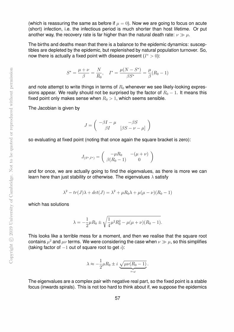
Cop
yri
ght
c ©20
19U
niv
ersi
tyof
Cam
bri
dge
.N
otto
be
quot
edor
repro
duce
dw
ithou
tp
erm
issi
on
(which is reassuring the same as before if µ = 0). Now we are going to focus on acute(short) infection, i.e. the infectious period is much shorter than host lifetime. Or putanother way, the recovery rate is far higher than the natural death rate: ν � µ.
The births and deaths mean that there is a balance to the epidemic dynamics: suscep-tibles are depleted by the epidemic, but replenished by natural population turnover. So,now there is actually a fixed point with disease present (I∗ > 0):
S∗ =µ+ ν
β=N
R0
, I∗ =µ(N − S∗)
βS∗=µ
β(R0 − 1)
and note attempt to write things in terms of R0 whenever we see likely-looking expres-sions appear. We really should not be surprised by the factor of R0 − 1. It means thisfixed point only makes sense when R0 > 1, which seems sensible.
The Jacobian is given by
J =
(−βI − µ −βS
βI [βS − ν − µ]
)so evaluating at fixed point (noting that once again the square bracket is zero):
J(S∗,I∗) =
(−µR0 −(µ+ ν)
β(R0 − 1) 0
)and for once, we are actually going to find the eigenvalues, as there is more we canlearn here than just stability or otherwise. The eigenvalues λ satisfy
λ2 − tr(J)λ+ det(J) = λ2 + µR0λ+ µ(µ− ν)(R0 − 1)
which has solutions
λ = −1
2µR0 ±
√1
4µ2R2
0 − µ(µ+ ν)(R0 − 1).
This looks like a terrible mess for a moment, and then we realise that the square rootcontains µ2 and µν terms. We were considering the case when ν � µ, so this simplifies(taking factor of −1 out of square root to get i):
λ ≈ −1
2µR0 ± i
√µν(R0 − 1)︸ ︷︷ ︸
=ω
.
The eigenvalues are a complex pair with negative real part, so the fixed point is a stablefocus (inwards spirals). This is not too hard to think about if, we suppose the epidemics
57

Cop
yri
ght
c ©20
19U
niv
ersi
tyof
Cam
bri
dge
.N
otto
be
quot
edor
repro
duce
dw
ithou
tp
erm
issi
on
happen and then host turnover refills S gradually. From these considerations, we candraw a phase diagram, and typical dynamics against time:
�
�����
�
�I have cheated here to make the diagrams a bit clearer. On the left, I have scaled S downsomewhat to fit it on same plot. On right, I’ve taken a different ν : µ ratio, to move the fixed
point away from the S axis, so swirly dynamics is clearer.
This is like a damped pendulum, settling down to some endemic equilibrium. Lookingat the these epidemics as we settle down, we can work out their approximate periodfrom the imaginary part of the eigenvalues. The dynamics will be like cos(ωt), andsome decaying exponential. So the period T is
T ≈ 2π
ω=
2π√µν(R0 − 1)
and it is of note that (µν)−12 is just the geometric mean of host lifetime and disease
infectious period. The R0 − 1 is back again. If R0 is only just above threshold, theperiod between epidemics is large. If R0 is huge, then short period (bit like a pendulumin very strong gravity).
To finish the measles story, here we have period epidemics settling down. But reallife is not like this model in one crucial way. The dynamics of measles in UK beforevaccination involved much of the spread being in school-age children. And of coursethen, we should think about how schools worked. Kids aged 5 or so start schooltogether in September, at the start of their first academic year. So, rather than therebeing a gentle trickle of susceptibles into the system, there is a huge kick once a year.This is enough to stop our damped pendulum settling down. The estimated T formeasles (using the expression above, put R0 = 20, infectious period about 12 days,lifetime about 70 years) is about 2.18 years. The forcing rounds this to a whole numberof years, and so we end up with our epidemics every two years.
The author of these notes is probably biased (this is JRG’s research area), but the fieldof disease modelling is very rich in terms of both mathematical interest and practical
58

Cop
yri
ght
c ©20
19U
niv
ersi
tyof
Cam
bri
dge
.N
otto
be
quot
edor
repro
duce
dw
ithou
tp
erm
issi
on
importance. However, we have some other interesting topics to cover in this course,so we will move on. If you want to read more, then do have a look at the book called‘Modeling Infectious Diseases in Humans and Animals’ by Keeling and Rohani. end of
lecture 9
1.3.5 Excitable systems
In this section we consider excitable systems where a biological system can ‘fire’ fol-lowing a small impulse. Heart muscle cells are one example of this: these are primedto contract in response to small electrical impulses. At the huge scale we could alsoconsider large population phenomena such as plankton blooms, where relatively smallenvironmental effects can lead to a dramatic burst of plankton growth. Arguably, someepidemic models should be considered also as excitable systems: a small number ofinitial infecteds can spark off a major epidemic. However for contrast here we will focuson a small physiological system: a neuron (nerve or brain cell) which receives a smallinput signal and can then fire an onwards signal to other cells.
The biochemical basis for signal propagation by neurons is well understood. It comesdown to considering the difference in electrical potential (voltage) between the insideand outside of the cell, and how positively charged sodium and potassium ions aretransported across the membrane by pumps. These pumps themselves change theirbehaviour according to the voltage difference. It is possible to develop a set of equa-tions to represent these quantities (the Hodgkin-Huxley model of the action potential).While this system behaves in the right sort of way, it is not very easy to use it to gainmathematical insight as to why there is a threshold where an initial impulse is largeenough to cause a ‘spike’.
Here we move to a second layer of models (so this is a really a model of a model35).This type of model was developed independently by two researchers, hence it is theFitzhugh-Nagumo model. Students of dynamical systems will see similarities with thevan der Pol oscillator, but this has a subtle but important modification.
Here is the Fitzhugh-Nagumo model:
u = c
(v + u− 1
3u3 + z(t)
)v = −1
c(u− a+ b v)
where0 < b ≤ 1, 1− 2
3b < a < 1, c� 1 .
The term z(t) represents external input, which might be applied at some time and notat others. To start with, we analyse the system with z(t) = 0. Note that the u and v are
35one could argue it is actually models all of the way down: the Hodgkin-Huxley model is itself a simplemathematical description of our understanding of the electrochemistry, and of course our understandingis an idealised model of how some imagined neuron might fire, and ‘neuron’ is catch-all term for a varietyof cells, and so it goes on until we are in the land of philosophy, which means we probably should havestopped a while back, probably before reading this footnote.
59

Cop
yri
ght
c ©20
19U
niv
ersi
tyof
Cam
bri
dge
.N
otto
be
quot
edor
repro
duce
dw
ithou
tp
erm
issi
on
not quantities that we can easily relate back to the original biochemical model: theyare not directly comparable to potassium levels, voltage difference or other physicalquantities, but the idea is that this model will illustrate the mathematical processes atwork.
The nullclines are themselves fairly simple (u on horizontal axis, v on vertical):
u = 0 : v = −u+1
3u3
-� �
- �
�
�
�
v = 0 : v =a− ub
-� ��-�
�
However we must check how they sit relative to each other. Given the v = 0 nullcline(in purple above) has gradient −1/b it is not too hard to check this is steeper than thedownwards section of the u = 0 nullcline. So there must be a single intersection. Therange in a above is rigged to ensure that at u = 1 the v = 0 nullcline is between −2/3and 0.
For c � 1, we have fast-slow dynamics again. The u dynamics are fast and so wemove quickly near-horizonal away from the u = 0 nullclines. The vertical adjustmenthappens more slowly. This means we crawl along just outside the cubic nullcline muchof the time, but if we reach the maximum or the minimum, then we ‘fall off’ and zipacross until we hit another section of the cubic.
�
For this plot, a = 0.7, b = 1 and c = 5.
60

Cop
yri
ght
c ©20
19U
niv
ersi
tyof
Cam
bri
dge
.N
otto
be
quot
edor
repro
duce
dw
ithou
tp
erm
issi
on
Same parameters, just a zoom-in on the fixed point showing how all trajectories head to it.
Depending on where we start, we might first do a stint moving up the left side of thecubic, then a hop across, and then drift down to the single fixed point. Unlike the vander Pol oscillator, that’s it! So long as z(t) = 0 we just stay there.
Finding the value of u and v at the fixed point involves solving a cubic of course, butluckily we do not actually need to do this. It suffice to say the fixed point is at (u∗, v∗) andto note that by the arrangement of nullclines, we see that u∗ > 1. Check the Jacobianat the fixed point to confirm stability (though we are already sure it must be stable):
J(u∗,v∗) =
(c (1− u∗2) c−1/c −b/c
)=
(− +− −
)which is clearly a matrix with negative trace and positive determinant, so indeed thefixed point is stable.
Suppose now that the system has settled to the fixed point, i.e. suppose the neuronis at rest. Now apply some input: z(t) = −V0, where V0 is a (possibly small) positiveconstant. We can see that the v = 0 nullcline is completely unchanged, but the u = 0nullcline shifts up by that constant. There are now three cases we must consider. Ineach of the plots for the cases below, the original cubic nullcline is shown in blue, andthe new shifted one in red, with the new fixed point in red. For the phase diagrams onthe left, the axes have been left out for clarity. The plot on the right shows v againsttime.
(i) No spike:
61

Cop
yri
ght
c ©20
19U
niv
ersi
tyof
Cam
bri
dge
.N
otto
be
quot
edor
repro
duce
dw
ithou
tp
erm
issi
on
����
�
Quite a dull case: basically the fixed point has not moved too much and the system justcorrects to the new system (same for V0 < 0).
(ii) Enough impulse for one spike:
����
�
This is the excitable behaviour! The trajectory from the old fixed point skims below thenew nullcline and thus has to go the whole way across to the other branch of the cubic,
climb up and then back to the right and climb down. This corresponds to spike in v. Afterthat, we arrive at the new fixed point, which is much as before.
(iii) Enough impulse for multiple spikes:
62

Cop
yri
ght
c ©20
19U
niv
ersi
tyof
Cam
bri
dge
.N
otto
be
quot
edor
repro
duce
dw
ithou
tp
erm
issi
on ����
�
Now V0 is large enough that it is actually a structural chance to the system. The new fixedpoint is not stable: the nullcline is now shifted so far that the fixed point has moved beyond
the minimum to the middle portion of the cubic. So, we start off as in case (ii): from theoriginal fixed point and do a loop, but now there is no fixed point to land on, so it goesaround again, and again, and again. It will keep going until z(t) is switched off again.
Exercise 27: Find the threshold for V0 for repeated firing (case (iii)).
So this Fitzhugh-Nagumo model illustrates how a mathematical system can be ex-citable. We can gain the insight that we need a nullcline which is like a cubic, withmultiple branches for a fast-slow solutions to follow. We can also see how a smallexternal input can shift the system so that there is a large single transient, or evenso that the system itself has changed and there are cycles. The fast-slow dynamicsmake it easy to illustrate what is going on, but it turns out that a large value of c is notrequired36. end of
lecture 10
36Have a go with the mathematica simulation.
63

Cop
yri
ght
c ©20
19U
niv
ersi
tyof
Cam
bri
dge
.N
otto
be
quot
edor
repro
duce
dw
ithou
tp
erm
issi
on
2 Stochastic systems
2.0 Preliminaries
2.0.0 Revision: discrete probabilities and generating functions
We will be considering discrete systems where the population size takes non-negativeinteger values (0, 1, 2, 3, . . .). This could be representing the number of individuals, cells,or perhaps molecules. We will usually37 write the random variable as N and particularvalues it takes as n.
P (n, t) = Probability(N = n at time t)
For clarity, often we will use the simpler notation of pn to mean P (n, t) when it is unam-biguous. As N can only take positive integer values, summing probabilities over all ofthese values:
∞∑n=0
pn = 1 .
We will also be making extensive use of generating functions:
φ(s, t) =∞∑n=0
snp(n, t) =∞∑n=0
snpn = 〈sN〉
Where the angle brackets 〈.〉 denote the expected value. Given a generating func-tion, we can recover pn by looking for the coefficient of sn. Recall some of the usefulproperties of generating functions, particularly by evaluating at special values of s:
φ(1, t) =∞∑n=0
pn = 1
φ(0, t) = p0 = Probability that the population has died out
We can also differentiate with respect to s:
∂
∂s
∣∣∣∣t
φ = φs =∞∑n=0
nsn−1pn
and from now on take partial derivatives with respect to s to mean t treated as constant,and vice-versa. And using this derivate of the generating function we can find the meanby evaluating at s = 1:
φs(1, t) =∑
npn = 〈N〉 = mean pop. = µ
37I will try to stick to this throughout these notes just for the sake of clarity (capitals for the randomvariable, lower case for the number it takes in an equation, usually as an index being summed over),but usually easy to interpret what is meant in any given expression, so not essential to be super carefulabout all this.
64

Cop
yri
ght
c ©20
19U
niv
ersi
tyof
Cam
bri
dge
.N
otto
be
quot
edor
repro
duce
dw
ithou
tp
erm
issi
on
(where µ is just the most commonly used letter for the mean). We do not need to besuper careful about putting limits on the sums so long as we say pn = 0 for n < 0.Differentiating a second time then evaluating at s = 1:
φss(1, t) =∑
n(n− 1)pn = 〈N(N − 1)〉 = 〈N2〉 − 〈N〉 = 〈N2〉 − µ
and recall the variance is given by
V ar(N) =⟨(N − µ)2⟩ =
⟨N2 − 2µN + µ2
⟩= 〈N2〉 − 2µ〈N〉+ µ2 = 〈N2〉 − µ2
We know µ from the generating function already, so we now have variance:
V ar(N) = φss(1, t) + µ− µ2 .
2.0.1 Why bother?
So far, we have only considered deterministic systems, and also we have focussedon continuous variables for things like population size. We know that we are doingthis for convenience of course. The number of individuals in a population should be anon-negative integer. To some extent, all biological processes are subject to randomfluctuations. However by taking these simplifications, we are in a realm where wehave a great deal of mathematical machinery we can use (differential equations, anddynamical systems in general). It means we can write down models and explore themwithout much difficulty. We can also understand them clearly enough to gain insightswhich often extend far beyond the particular model we have in front of us. We might beconfident that some of our results (for example the concept of R0 in disease dynamicsand hence the idea of a vaccination threshold) will hold even if we were to add morelayers of complexity to the models.
However, what have we missed by ignoring random fluctuations and forcing populationnumbers to be continuous? Perhaps the most obvious problem is that populations thatare decaying and getting very small still cannot ever reach zero, e.g.:
dN
dt= −λN =⇒ N = N0 e
−λt
(λ > 0) and even as t becomes very large, still N is positive. Does this matter? Well,yes it does if something changes later and the population size, which should have beenzero, can claw its way back from tiny numbers to being large.
A classic case of this was in a model for rabies in foxes proposed by Murray and others.In a published paper: the scenario of a rabies introduced to the south of England wasexplored by a deterministic diffusion model. As one might expect, rabies spreads outalmost radially over a few years. However it doesn’t end there: after some years,rabies reappears from the same initial location and spreads out again (though lessdramatically). This second introduction was not put in there by the modellers, but
65

Cop
yri
ght
c ©20
19U
niv
ersi
tyof
Cam
bri
dge
.N
otto
be
quot
edor
repro
duce
dw
ithou
tp
erm
issi
on
just happens in the simulations. This was explained by Mollison in a paper in 199138:the density of infected foxes at the origin location never actually died down to zero,though it did get to a very small value: 10−18 of a fox per square kilometre. Anyonereasonable would describe this as essentially no rabid foxes, but mathematically it isstill a quantity that can grow back when conditions allow (renewed susceptibility whenthe fox population has turned over for a few years). This Mollison called the ‘atto-fox’,and this has become a useful term to describe this modelling issue39. Note that thisis not a numerical issue from inaccuracy in computation, but one which comes fromthe very nature of continuous population deterministic models. Does this mean thatoriginal model was worthless? I would argue it still has use, but attention to resultsfrom simulations should stop after the first wave.
So although we do not always need to use stochastic models, we should be vigilant foratto-foxes and other artifactual effects in our deterministic models. And to watch outfor these effects, we must be aware of what they can be. As well as this issue withsmall numbers not going to zero, we can already guess (from thinking about excitablesystems already studied) that in some special situations, small fluctuations can lead tolarge effects. Further, we also do not always expect ‘average’ behaviour to in fact berepresentative of typical behaviours. In addition, we will see in the later parts of thissection that small fluctuations in two quantities are not always just independent noise:they can actually covary if the dynamics are interlinked.
2.0.2 The first step
Consider first this very simple system: we have states A and B only, and we are alwaysin exactly one of those states. We jump from A to B at probability rate λ. We can makea diagram like this:
� �
λ
Where dots (or nodes) denote states, arrows are the possible ‘jumps’ and the arrowsare labelled with the rates. There are two ways to proceed from here. The less formalapproach (taken in lectures) is simply to go from the diagram to consider flows ofprobability, an idea which might be familiar from continuous time Markov Chains fromIb . For completeness, the slightly more formal way is included in these notes in blue.If the more formal approach helps you understand things better than great, if not thenthen you can safely skip it. In both approaches, we introduce notation P (A, t) to meanprobability we are in state A at time t.
38Mollison, D. Dependence of epidemic and population velocities on basic parameters. 1991, Mathe-matical biosciences 107 (2)
39I have also heard this phenomena described as ‘nano-hawks’
66

Cop
yri
ght
c ©20
19U
niv
ersi
tyof
Cam
bri
dge
.N
otto
be
quot
edor
repro
duce
dw
ithou
tp
erm
issi
on
More formal What does probability rate λ actually mean? Essentially it is a probabil-ity per unit time of making a jump so that for small δt:
P ( jump by t+ δt | in A at time t) = λ δt+O(δt2)
One could justify this by essentially saying this is the definition of probability rate (a bitlike a probability density function f(x) dx). But perhaps more intuitive is to think of it asbeing an instantaneous rate λ until it happens. It might have already happened in δt sothen the rate is no longer λ. In fact that helps us to see why the correction is order δt2.
We can build up a differential equation for the probability by considering the probabilityof being in A at time t + δt conditional on each of the possibilities at time t, and whathappens in the time period between of length δt:
P (A, t+ δt) = P (A, t)P (stayed in A for δt) + P (B, t)P (went from B to A in δt)
= P (A, t) [1− P (left A during δt)] + P (B, t) [0]
= P (A, t) [1− λ δt] +O(δt)2
Then strategic rearrange and divide by δt:
P (A, t+ δt)− P (A, t)
δt= −λP (A, t) +O(δt)
and taking the limit δt→ 0:d
dtP (A, t) = −λP (A, t)
Alternatively, working straight from the diagram, it would not be unreasonable to godirectly for the same equation immediately, i.e.
d
dtP (A, t) = −λP (A, t) .
We can build a similar differential equation for P (B, t), but we do not need it as in factwe must be in A or B, so P (A, t) + P (B, t) = 1
We can solve this if we have an initial condition. Let us suppose we are at A initially soP (A, 0) = 1:
P (A, t) = e−λt
and hence alsoP (B, t) = 1− e−λt .
This rather unsurprising result lets us quickly check the distribution of times to jump.Let T be the time when we jump from state A to B. Then we can find the cumulativedistribution for T by noting we are in B if T has passed already:
P (T < t) = P (B, t) = 1− e−λt
67

Cop
yri
ght
c ©20
19U
niv
ersi
tyof
Cam
bri
dge
.N
otto
be
quot
edor
repro
duce
dw
ithou
tp
erm
issi
on
We can use this to find the probability density function:
f(t) =d
dt(1− e−λt) = λe−λt
which by now we see is the exponential distribution. And as always:∫ ∞0
f(t) dt = 1 .
We can find the expected jump time
〈T 〉 =
∫ ∞0
tf(t) dt =1
λ
and the variance of the jump time
V ar(T ) = σ2 = 〈T 2〉 − 〈T 〉2 =
∫ ∞0
t2f(t) dt− 1
λ2=
1
λ2.
and we could square root this for the standard deviation σ and we see that it is equalto the mean.
2.1 Discrete population sizes
2.1.1 Single populations
We now study the pure import model. There is a probability rate λ of adding oneindividual to the population, no matter what the current population size is. We startwith zero population. Again, represent states as dots and jumps as arrows:
λ λ λ λ λ λ λ
� � � �-� � �+�����
λ λ λ λ λ λ λ
And writing P (n, t) to mean probability of the population size (N ) being n at time t, thenthe initial condition just says that P (0, 0) = 1 and P (n, 0) = 0 for n > 0.
Again we can set things up by considering were we are at t+ δt starting from t:
P (n, t+ δt) = P (n, t)× (1− λδt+O(δt2)) + P (n− 1, t)× (λδt+O(δt2)) +O(δt2) .
In theory we should be including a term for every possible previous state on the righthand side here, but that last O(δt2) takes care of all of the others. For example, startingfrom n− 2 we would have to jump twice during δt to end up in n. Other states are evenmore remote, or even impossible to get to n: that last O(δt2) is a big bin for them all.
68

Cop
yri
ght
c ©20
19U
niv
ersi
tyof
Cam
bri
dge
.N
otto
be
quot
edor
repro
duce
dw
ithou
tp
erm
issi
on
As before, rearrange and divide by δt to prepare for a derivative:
P (n, t+ δt)− P (n, t)
δt= −λP (n, t) + λP (n− 1, t) +O(δt) .
Take the limit δt→ 0.
Or again, work directly from the diagram:
d
dtP (n, t) = λP (n− 1, t)− λP (n, t)
and at this point it would be sensible to use the shorter notation pn = P (n, t):
pn = λ(pn−1 − pn) (17)
and we can say this holds for all n ≥ 0 by the nice convention of saying pn = 0 for n < 0.
Equation (17) is an example of a master equation, which is just a fancy way of sayinga differential equation for pn. It is a slightly curious object though as it is (continuous)differential equation in t, but a (discrete) difference equation in n.
In this case, we see that the master equation gives a system of differential equationsthat we can actually fully solve explicitly.
Exercise 28: Set p0 = 1, pn = 0 for n > 0 at t = 0. Solve the master equationinductively to get
pn =(λt)n
n!e−λt
Generally we cannot fully solve in this way, in which case it is often a good idea to try agenerating function. Recall:
φ(s, t) =∞∑n=0
snpn = 〈sN〉
Then we can differentiate φ with respect to t (keeping s fixed), and substitute in usingthe master equation:
∂φ
∂t=∑
snpn =∑
snλ(pn−1 − pn) = λ∑
sn pn−1 − λ∑
sn pn
= λ∑
sn+1 pn − λ∑
snpn
= λ s φ− λφ= (s− 1)λφ
And we can integrate this (remember that s was treated as a constant):
φ = A(s)e(s−1)λ t
69

Cop
yri
ght
c ©20
19U
niv
ersi
tyof
Cam
bri
dge
.N
otto
be
quot
edor
repro
duce
dw
ithou
tp
erm
issi
on
To resolve A(s), consider t = 0:
φ(s, 0) =∑
snpn(0) = p0(0) + s p1(0) + s2 p2(0) + s3 p3(0) + . . .
and p0(0) = 1 and the rest of the pn(0) = 0 for n > 0, so φ(s, 0) = 1. And from this wesee that A(s) = 1 for all s. So here we have the full solutions for the generating function
φ(s, t) = e(s−1)λ t
Great. So what can we do with φ? Well, it encodes all of the pn, so we could useit to recover the pn by taking the coefficient of sn. This we could do by Taylor series(recognition or differentiating n times and evaluating at s = 0):
pn = Coef of sn in φ = Coef of sn in e−λ teλ ts
= Coef of sn in e−λ t(
1 + (λts) +1
2!(λts)2 + . . .+
1
n!(λts)n + . . .
)= e−λ t
(λt)n
n!
Often we are not very interested in pn itself, but rather want things like the mean andvariance, which can be found directly without having to go via the pn. For the mean:
µ = 〈N〉 =∂φ
∂s
∣∣∣∣s=1
= λ t e(s−1)λ t∣∣s=1
= λ t
and for the variance:
〈N(N − 1)〉 =∂2φ
∂s2
∣∣∣∣s=1
= (λ t)2 e(s−1)λ t∣∣s=1
= (λ t)2
so
σ2 = V ar(N) = 〈N2〉 − 〈N〉2 =∂2φ
∂s2
∣∣∣∣s=1
+ µ− µ2 = (λ t)2 + (λ t)− (λ t)2 = λ t .
This could be used to say something about the size of small fluctuations. Typical fluc-tuations are of the order of the standard deviation σ =
√λ t. Typical population sizes
are of the order of the mean µ = λ t, so relative to population size, fluctuations go like(λ t)−1/2 so fluctuations become less important for this system as time goes on.
One further note on this simple import system: if we were to construct an analogousdeterministic system, it would surely be
dN
dt= +λ
and with N(0) = 0 the solution would be N = λ t. This agrees with the mean of thestochastic system. Note: this agreement does not always hold40.
40You might like to try and identify what is special about this system. It might help to think about forwhat functions f is it true that 〈f(N)〉 = f(〈N〉) .
70

Cop
yri
ght
c ©20
19U
niv
ersi
tyof
Cam
bri
dge
.N
otto
be
quot
edor
repro
duce
dw
ithou
tp
erm
issi
on
Import and death model Here we use the same model for import (probability rateλ of adding a new individual, including when at n = 0). Now we add a per capitaprobability rate of death β so the total rate is β n:
�-� � �+�
λ λ
β � β (�+�)
By now, we should be able to build the master equation by considering ‘flows’ of proba-bility between states (the approach with δt would be fine but rather tedious). Focussingon state n in the diagram above, we can see two arrows going in and two going out,giving us the four terms: end of
lecture 12pn = λpn−1 − λpn + β(n+ 1)pn+1 − βnpn
= λ (pn−1 − pn) + β [ (n+ 1) pn+1 − n pn]
Here, we go straight for the equation satisfied by the generating function:
∂φ
∂t=∑
snpn = λ∑
sn pn−1 − λ∑
sn pn + β∑
sn (n+ 1) pn+1 − β∑
sn n pn
and as always, it is a good idea to split into separate sums, so we can shift the indexon each one separately, aiming for pn in each:
∂φ
∂t= λ
∑sn+1 pn − λ
∑sn pn + β
∑n sn−1 pn − β
∑n sn pn
The first two sums are much as before (sφ and φ), but for the latter two, we mustdifferentiate φ with respect to s to get the bonus n in the coefficients to appear:
∂φ
∂s= φs =
∑n sn−1 pn
so we can immediately recognise the third sum as φs. The fourth one is the same thingagain but with a spare factor of s:
∂φ
∂t= λ s φ− λφ+ βφs − β s φs
and we can factorise41 out (s− 1) to get
φt = (s− 1) [λφ− β φs] (18)
We should also specify an initial condition. Again we will take N = 0 initially so thatφ(s, 0) = 1.
41This keeps happening and should not be a surprise. We know that φ = 1 for s = 1, so φt = 0 fors = 1.
71

Cop
yri
ght
c ©20
19U
niv
ersi
tyof
Cam
bri
dge
.N
otto
be
quot
edor
repro
duce
dw
ithou
tp
erm
issi
on
Exercise 29: Get from the dots, arrows and rates diagram above to equation(18) without lecture notes
We can actually fully solve for φ again in this case. Take a strategic form:
φ = e(s−1)f(t)
where f(t) is a function yet to be determined and substitute into equation (18):
(s− 1)f ′(t)φ = (s− 1) [λφ− βf(t)φ]
and then it is clear that this form was designed to cancel the (s−1)φ and we’re left witha DE in purely f :
f ′(t) = λ− βf(t) =⇒ f(t) =λ
β+ Ae−β t
The initial condition that φ = 1 at t = 0 corresponds to f(0) = 0, and this determines A,which fully determines f and hence we have
φ(s, t) = eλβ
(s−1)(1−e−βt)
and the double exponential might not be pretty, but it is nice to have fully solved for φ.
Exercise 30: Use this φ to show that the mean is given by
〈N〉 =λ
β(1− e−βt)
and the variance is actually the same
V ar(N) =λ
β(1− e−βt)
Suppose we are now interested in what happens to this system at large time, so weare looking for a steady state solution and not worrying about initial condition. Wecould use our solution and let t → ∞. However, to illustrate a more generally usefultechnique we will suppose that we do not actually have the solution for φ. We can goback to equation (18) and seek the solution that is independent of time (i.e. set φt = 0):
0 = (s− 1) [λφ− β φs]
which is just a DE for φ in s, which we can solve:
φs =λ
βφ =⇒ φ = Ae
λβs
72

Cop
yri
ght
c ©20
19U
niv
ersi
tyof
Cam
bri
dge
.N
otto
be
quot
edor
repro
duce
dw
ithou
tp
erm
issi
on
and we cannot use the time initial condition here, but need something for a fixed valueof s. The one to go for here is always φ = 1 at s = 1. So A = e−
λβ and we have the
steady state solution for φ:φ = e
λβ
(s−1)
and we see this is reassuringly consistent with what we would get with t → ∞ in thegeneral solution above.
We can also quickly see the steady state pn by pulling out the appropriate coefficientof sn:
pn = Coef of sn in φ = e−λβ
(λ
β
)n1
n!
(which we recognise as the Poisson distribution).
Aside on simulations
As always, it helps build intuition for what this is all about by looking at the output ofsimulations to get a feel for how these things behave. Here’s one for this import anddeath model from this last section with λ = 20 and β = 1:
5 10 15 20�0
5
10
15
20
25
30
�λ=��� β=�
The dotted line is λ/µ = 20, what we expect the mean to settle to. Indeed you can seethat it heads quickly away from the initial condition and bumbles around near the mean.
73

Cop
yri
ght
c ©20
19U
niv
ersi
tyof
Cam
bri
dge
.N
otto
be
quot
edor
repro
duce
dw
ithou
tp
erm
issi
on
You could even say the standard deviation looks to be about 4 or 5, which is consistenttoo with long term behaviour (σ =
√20).
This programming approach is certainly not examinable, but it is actually very easy tosimulate models like these. The Gillespie algorithm is both simple to code and fast torun. It relies on some nice properties of the exponential distribution. Suppose currenttime is ti and population size is ni. Then from the model we have some probability ratesfor jumps to other states. Each of these possible jumps happens at exponentially dis-tributed time, but only the first one is actually the one that happens. The nice propertyis that the time for the first of a bunch of exponential distributions is itself an exponentialdistribution, with rate just sum of the others. Simulating an exponential distribution issuper easy: just pick uniform random real in (0, 1), take minus log of it, and divide byrate.
Then which event is it that happens? Also easy to run: just pick another uniformrandom and use it to choose event by weighting the unit interval in proportion to therates of each possible event. Then you have ti+1 = ti + ∆t and ni+1 is whatever it isafter the chosen event.
Then rinse and repeat a number of times, but how many? Can either do a set numberof events (some max for i), or until time is above some threshold (some max for t), butneed to check some event is possible, i.e. total rate has not hit zero (rtot 6= 0). That lastpossibility can’t happen in this model, but could in others later, if we are in some stuckstate (extinction, below). Here it is as pseudo code for this model: start with i = 0,choose some n0 and probably t0 = 0:
• Loop back to here, got ni, ti at some step i
• Compute rates for events rb = λ, rd = βni. Total rate rtot = rb + rd.
• Generate a couple of uniform (0, 1) random numbers: random1, random2
• Time to next event ∆t = − log(random1)/rtot
• Choose which event: if random2 < rb/rtot it is a birth, else a death
• update variables: ti+1 = ti + ∆t and ni+1 = ni + 1 if birth, ni+1 = ni − 1 if death
• i = i+ 1, loop back
Variance and step size
A generalisation of the import and death model allows us to see how the variance ofthe steady state depends on step size. The death rate is still β per capita, but now wesuppose that M individuals are added each time, rather than just one, but still at rateλ. (Take M to be some positive integer of course.) How do we expect the mean andvariance in steady state to change?
74
Cop
yri
ght
c ©20
19U
niv
ersi
tyof
Cam
bri
dge
.N
otto
be
quot
edor
repro
duce
dw
ithou
tp
erm
issi
on
�-� � �+��-� �+�
λ λ
β � β (�+�)
This works much as above, so let us jump straight to the master equation:
pn = λ (pn−M − pn) + β [ (n+ 1) pn+1 − n pn]
and then find the PDE satisfied by the generating function φ.
Exercise 31: Show∂φ
∂t= λ(sM − 1)φ− β(s− 1)φs
We could work directly with the generating function for example to find steady state:42
φt = 0 =⇒ φs =λ
β
(sM − 1
s− 1
)φ
And this would work well for any given M , as we’d just have a nice polynomial inthat bracket. But to illustrate another more general approach, suppose we couldn’tprogress with the generating function directly, then we could instead think of workingwith the master equation directly to find differential equations (in time) for the moments(expected N to some power):
d
dt〈N〉 =
∑n pn
= λ∑
n pn−M − λ∑
n pn + β∑
n(n+ 1) pn+1 − β∑
n2 pn
= λ∑
(n+M) pn − λ∑
n pn + β∑
(n− 1)n pn − β∑
n2 pn
= λ∑
M pn + β∑
(−n) pn
= λM − β〈N〉
where we have used the master equation to sub in for pn, and then expanded to writeone sum per p term, then shifted the index on each sum so the p term is pn, then ittidies from there. So this is a nice43 differential equation in 〈N〉. For initial condition, wesupposed N = 0 at t = 0, so also 〈N〉 = 0 at t = 0, and we can then easily solve:
42Do note that in stochastic models, steady state means that the pn are constant, not N . The generalbehaviour of the system has settled into something, not that the population size has settled to a fixedvalue.
43actually this all seems rather too nice, and you might be suspicious that there was something specialhere. Indeed there is! The birth and death rates were only linear in n, which means the coefficients inthe master equation are only linear. The equation for time derivative for each moment will end up beingjust in terms of that moment and lower. If birth or death rates were quadratic in n, we would find d
dt 〈N〉depends on 〈N2〉 and so on up, which means we no longer have a closed system.
75

Cop
yri
ght
c ©20
19U
niv
ersi
tyof
Cam
bri
dge
.N
otto
be
quot
edor
repro
duce
dw
ithou
tp
erm
issi
on
〈N〉 =λM
β(1− e−βt)
and we can also see 〈N〉 → λM/β as t→∞.
A similar approach with higher moments will also work:
d
dt〈N2〉 =
∑n2 pn
= λ(∑
n2 pn−M −∑
n2 pn
)+ β
(∑n2(n+ 1) pn+1 −
∑n3 pn
)= λ
∑((n+M)2 − n2
)pn + β
∑((n− 1)2n− n3
)pn
= λ∑(
2nM +M2)pn + β
∑(−2n2 + n
)pn
= λ(2〈N〉M +M2
)+ β
(−2〈N2〉+ 〈N〉
)= λM2 + (2λM + β)〈N〉 − 2β〈N2〉
and this also gives us a sensible DE as we already have solved to get 〈N〉 as a functionof time. If we write 〈N2〉 = X then we have a DE in this form:
X = −2βX + a+ b eβt
where the coefficients a and b are some constants that can be deduced from above.
Exercise 32: Show that at steady state
〈N2〉 =λ
2β
(1 +
2λ
β
)M2 +
λ
2βM .
Note, you have a choice here. Fast method (which would be fine) is to just usethe differential equation at steady state to find the equilibirum value directly.Full method (good for extra practice) is to fully solve the DE to get 〈N2〉 as afunction of t, and then let t→∞.
Either way... show also that if M � 1,
var(N) =λ
2βM2 .
Intuition and effect of step size: now think about the effect of changingM . Remem-ber that the model is to add M individuals at rate λ and they die at some per capitarate β. It is intuitive that the population will head towards some balance between intro-duction and death: if the population is much larger than this balance then death rate
76

Cop
yri
ght
c ©20
19U
niv
ersi
tyof
Cam
bri
dge
.N
otto
be
quot
edor
repro
duce
dw
ithou
tp
erm
issi
on
will dominate, if much smaller then the birth rate will dominate. So, this matches withexpected N being λM/β. We can also imagine that once the system is near that, thenit will just stay vaguely near, but some random fluctuations coming from the stochasticnature of the model.
Suppose now that we make M ten times as big, and shrink λ by a corresponding factorof 10. Then intuitively we have the same average rate of individuals being added, andindeed we see 〈N〉 is unchanged (proportional to λM ) . However, we see that thevariance (proportional to λM2 for large M ) will increase, and indeed ten times as muchif we started with large M . Hopefully, this will also seem intuitive: we’ve made thestochastic process more ‘lumpy’ by having a rarer but larger step. This idea will beuseful later!
0 10 20 30 40�0
50
100
150
200�
λ=���� β=� � �=�
0 10 20 30 40�0
50
100
150
200�
λ=��� β=� � �=��
Small M on left, large M on the right, also chaing λ to keep the mean constant. There’sclearly more variability with the larger M .
end oflecture 13
2.1.2 Extinction
The examples above had a constant import rate, so even when n = 0 there is a constantimmigration into the system. It turns out that this is crucial to get non-trivial steadystates. In models with a closed population, no immigration is possible, so there is noway to get from n = 0 to n = 1, and once the population has gone extinct, it stays thatway forever. In this section, we will build up some typical properties we might expectfrom a single population stochastic model, and we see that extinction is inevitable.
Here are three reasonable properties for a closed population model:
1. No births/immigration from n = 0
2. Death is possible for all n > 0
3. For large n, the death rate is much larger than the birth rate
77

Cop
yri
ght
c ©20
19U
niv
ersi
tyof
Cam
bri
dge
.N
otto
be
quot
edor
repro
duce
dw
ithou
tp
erm
issi
on
� � � �-� � �+�
����
�� ��-� ��
�� �� �� ��+�� � � �-� � �+�
����
Setting bn and dn to be birth and death rates respectively from state n, we can translatethese properties to something in terms of these rates:
1. b0 = 0
2. dn > 0 for all n > 0
3. Either bn = 0 for some n, or dn/bn � 1 for large n
We now divide into two cases to consider extinction:
(i) If bn = 0 for some n > 0: then the state space is actually finite (0, 1, 2, 3 . . . n− 1, n)so we can use a result from IB Markov Chains: if we have a finite state space and allstates communicate with n = 0, and n = 0 is absorbing (i.e. once we are there, we staythere), then as t→∞, p0 → 1. In other words, extinction is inevitable.
(ii) If bn > 0 for all n > 0: then we seem to have an infinite state space, but actuallythe same result turns out to be true. Perhaps this is almost intuitive if we rememberthat one of our conditions is that the death rate far outweighs birth rate large for large n,so it should behave as if the state space is effectively finite. But, here’s a slightly moremathematical argument (which of course uses that condition of deaths outweighingbirths). We set up qn the probability of extinction eventually, given we start at n. Thenwe can immediately have that q0 = 1 (this is instant game over: we started at zero).For n > 0, we set up a recurrence, again using law of total probability: if we’re at n > 0then either a birth or a death next. If there’s a birth, then we will be at n + 1 and theprobability of ultimate extinction starting from here is qn+1. Similarly for death next. So:
qn = P (birth next) qn+1 + P (death next) qn−1
and what is the probability of birth or death next? We have the rates bn and dn (andknow neither is zero in this case), so:
P (birth next) =bn
bn + dn, P (death next) =
dnbn + dn
.
Subbing these in, and multiplying through by total rate bn + dn:
(bn + dn)qn = bnqn+1 + dnqn−1
78

Cop
yri
ght
c ©20
19U
niv
ersi
tyof
Cam
bri
dge
.N
otto
be
quot
edor
repro
duce
dw
ithou
tp
erm
issi
on
Rearrange to split bn and dn:
bn(qn − qn+1) = dn(qn−1 − qn)
(qn − qn+1) =dnbn
(qn−1 − qn)
Note that we can’t immediately solve this recurrence with only one initial condition, butwe can argue through that there is only one feasible solution. Notice the bracket termsare just difference in consecutive qi, and this recurrence equation holds for all n > 0,so chase the bracket on the right down:
(qn − qn+1) =dnbn
(qn−1 − qn)
=dnbn
dn−1
bn−1
(qn−2 − qn−1)
=dnbn
dn−1
bn−1
. . .d1
b1
(q0 − q1)
=
(n∏i=1
dibi
)(q0 − q1)
And again this holds for all n. Notice the LHS is the difference of two probabilities,so must be between -1 and 1 for all n. Consider the product on the RHS and takinglarger and larger n. We can make this product as large as we like44. Obviously (q0−q1)doesn’t depend on n, but that equation holds for all n, so the only possibility we are leftwith is q0 − q1 = 0. So q1 = q0 = 1.
Now by the above equation, qn+1 − qn = 0 for all n > 0, so finally we have that qn = 1for all n. Extinction is inevitable, starting from any n. This completes the second case(infinite state space, but actually effectively finite state space).
It can be shown that a similar result holds for multiple populations. Think about a vectorfor replacing n, where the elements are population numbers for different species. Weshould still have similar conditions: the vector of zeros being absorbing, deaths in eachspecies being possible if any members are present, and very large populations beingsquished down by death rate outweighing the birth rate.
Treat this blue paragraph as starred, and ignore if it doesn’t help you... It is intuitive thatthe same sort of argument as above should work, but here’s a slightly different way tothink about it (not given in lectures): divide up the infinite state space into three: (i)extinction (all populations zero, a single state), (ii) all populations within sensible size(some very large but finite state space), (iii) at least one population ridiculously large(the rest of the infinite state space). Then think of the possible transitions betweenthese three states. State (iii) has death rates pushing us back towards (ii) and bycarefully choosing what we mean by ‘ridiculously large’ we could make conditions on
44and actually this tells us more precisely what we mean by death rate outweighing birth rate for largen. We can see that it would be enough to say dn ≥ Rbn for all n > n, for some n and some R > 1.
79

Cop
yri
ght
c ©20
19U
niv
ersi
tyof
Cam
bri
dge
.N
otto
be
quot
edor
repro
duce
dw
ithou
tp
erm
issi
on
birth/death rates that give finite expected time until we are back in (ii). From state (ii)we can go to (iii) or (i), and as there are finitely many states, we pop out one way orthe other in finite time. Obvious in (i) we stay there. So now we have something similarto a three state Markov chain with single absorbing state, and the other two statescommunicate with it. Hence, we will end up there with probability 1.
However, for single or multiple populations, the expected time to extinction could beextremely large45
2.1.3 Multiple populations
Here we are going to look at a stochastic model with two populations: wildebeest(represented by m) and flies (n). This model is a bit unusual in that we are going tohave the wildebeest affecting the dynamics of the flies, but not vice versa. This is nottypical, but means we can handle the mathematics fairly easily, and be able to see theconsequence of the interactions clearly on the flies.
The wildebeest have population size m, and ‘births’ are rate λ1 (i.e. this is the importmodel above, so no longer worry about extinction) and deaths at rate β1m (so β1 percapita). The flies have population size n, ‘birth’ rate λ2m, and death rate β2n. The weirdbit here is that the birth rate is proportional to the number of wildebeest. This is notbecause wildebeest give birth to flies, but interpret it here as a kind of import rate, andthe flies are attracted by the wildebeest. The more wildebeest there are, the higher therate of flies that join the system.
The current state of the system is given by (m,n), which we can think of as correspond-ing to grid coordinates. Then we could do our arrows diagram like this:
45It might seem alarming that any stochastic model like this leads to total extinction always, and onemight start fretting that life on earth could in principle be represented by such a system, and compli-cations like time-dependence from days and seasons could be ironed out. However, there is a bigdifference between it being a mathematical inevitability, and it being something to actually lose sleepover. Expected time could be orders of magnitude larger than the age of our solar system. The‘end of life on earth’ is not on my personal worry list. Extinction of individual species, however, is.If this also interests you, please do go and think and read more on this. Here’s one starting point:https://www.durrell.org/wildlife/wildlife/durrell-index/explore/ .
80
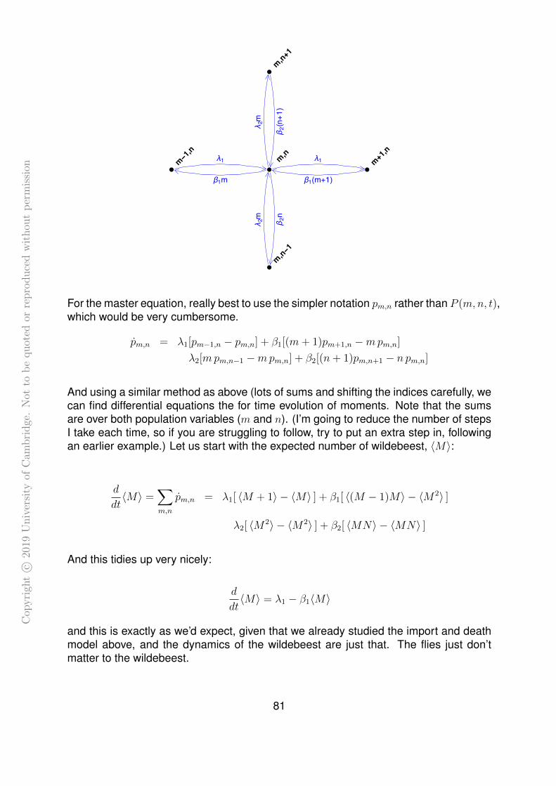
Cop
yri
ght
c ©20
19U
niv
ersi
tyof
Cam
bri
dge
.N
otto
be
quot
edor
repro
duce
dw
ithou
tp
erm
issi
on
���
�+���
�-���
���-�
���+�
λ� λ�
β�� β�(�+�)
�
�
�
β�(�+�)
For the master equation, really best to use the simpler notation pm,n rather than P (m,n, t),which would be very cumbersome.
pm,n = λ1[pm−1,n − pm,n] + β1[(m+ 1)pm+1,n −mpm,n]
λ2[mpm,n−1 −mpm,n] + β2[(n+ 1)pm,n+1 − n pm,n]
And using a similar method as above (lots of sums and shifting the indices carefully, wecan find differential equations the for time evolution of moments. Note that the sumsare over both population variables (m and n). (I’m going to reduce the number of stepsI take each time, so if you are struggling to follow, try to put an extra step in, followingan earlier example.) Let us start with the expected number of wildebeest, 〈M〉:
d
dt〈M〉 =
∑m,n
pm,n = λ1[ 〈M + 1〉 − 〈M〉 ] + β1[ 〈(M − 1)M〉 − 〈M2〉 ]
λ2[ 〈M2〉 − 〈M2〉 ] + β2[ 〈MN〉 − 〈MN〉 ]
And this tidies up very nicely:
d
dt〈M〉 = λ1 − β1〈M〉
and this is exactly as we’d expect, given that we already studied the import and deathmodel above, and the dynamics of the wildebeest are just that. The flies just don’tmatter to the wildebeest.
81
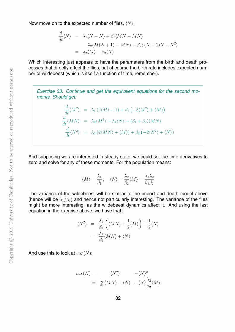
Cop
yri
ght
c ©20
19U
niv
ersi
tyof
Cam
bri
dge
.N
otto
be
quot
edor
repro
duce
dw
ithou
tp
erm
issi
on
Now move on to the expected number of flies, 〈N〉:
d
dt〈N〉 = λ1〈N −N〉+ β1〈MN −MN〉
λ2〈M(N + 1)−MN〉+ β2〈 (N − 1)N −N2〉= λ2〈M〉 − β2〈N〉
Which interesting just appears to have the parameters from the birth and death pro-cesses that directly affect the flies, but of course the birth rate includes expected num-ber of wildebeest (which is itself a function of time, remember).
Exercise 33: Continue and get the equivalent equations for the second mo-ments. Should get:
d
dt〈M2〉 = λ1 (2〈M〉+ 1) + β1
(−2〈M2〉+ 〈M〉
)d
dt〈MN〉 = λ2〈M2〉+ λ1〈N〉 − (β1 + β2)〈MN〉
d
dt〈N2〉 = λ2 (2〈MN〉+ 〈M〉) + β2
(−2〈N2〉+ 〈N〉
)
And supposing we are interested in steady state, we could set the time derivatives tozero and solve for any of these moments. For the population means:
〈M〉 =λ1
β1
, 〈N〉 =λ2
β2
〈M〉 =λ1λ2
β1β2
The variance of the wildebeest will be similar to the import and death model above(hence will be λ1/β1) and hence not particularly interesting. The variance of the fliesmight be more interesting, as the wildebeest dynamics affect it. And using the lastequation in the exercise above, we have that:
〈N2〉 =λ2
β2
(〈MN〉+
1
2〈M〉
)+
1
2〈N〉
=λ2
β2
〈MN〉+ 〈N〉
And use this to look at var(N):
var(N) = 〈N2〉 −〈N〉2
= λ2β2〈MN〉+ 〈N〉 −〈N〉λ2
β2
〈M〉
82

Cop
yri
ght
c ©20
19U
niv
ersi
tyof
Cam
bri
dge
.N
otto
be
quot
edor
repro
duce
dw
ithou
tp
erm
issi
on
var(N) = 〈N〉+λ2
β2
( 〈MN〉 − 〈M〉〈N〉 )
= 〈N〉+λ2
β2
cov(M,N)
recognising the second term as the covariance between M and N . We could thendescribe the flies variance as having two components: intrinsic variability from the firstterm, and extrinsic variability from the second term. The first term is just the fluctuationswhich come from the randomness of the flies own birth and death process directly. Ifwe somehow totally fixed the number of wildebeest and looked at the flies dynamics inisolation, the variance would just be the first term. The second term is to do with thenumber of wildebeest changing and thus moving the flies birth rate around.
Actually, if we look at a typical output of a simulation, it is possible to see that bothpopulations have fluctuations of course, but if the wildebeest numbers take a bit of adetour from the mean, then flies seem to follow suit. If we didn’t already know, we couldguess from this that the populations are interacting somehow.
5 10 15 20�0
20
40
60
80
100
�� �λ�=�� β�=� λ�=�� β�=�
One output of a Gillespie simulation of the model described above. The wildebeest M areplotted in red and the flies N in black. The means (as computed above) for each
population is marked with dotted horizontal line of appropriate colour. Look for a placewhere the red curve moves a bit away from the mean, and check the what happens to theblack curve. It should be that the flies population starts to drift in the same direction (from
increased or decreased birth rate) and thus flies curve is very variable: it has its ownintrinsic variability, but also it is being shoved around by the wildebeest fluctuations.
We will come back to these ideas again below, thinking about covariances in general.Here, we can see that we would expect M and N to be covarying positively. end of
lecture 1483

Cop
yri
ght
c ©20
19U
niv
ersi
tyof
Cam
bri
dge
.N
otto
be
quot
edor
repro
duce
dw
ithou
tp
erm
issi
on
2.2 Continuous population sizes
2.2.1 Fokker-Planck for a single variable
So far for stochastic models we have thought of the population size n as an integer.Hence we are dealing with master equations which are discrete in n (but continuous intime). Here, we recognise that these distributions ‘look like’ a continuous distribution, insome sense. This is particularly when the width of our distribution is much larger thanour typical step size (usually ±1). By convention and for clarity, when we think aboutcontinuous population sizes, we will write x rather than n, but these are really the samething. By making an approximation, we replace our master equation (discrete in n) witha Fokker-Planck equation (continuous in x). Watch carefully below for the moment ofapproximation!
To do all this, we should set up some general notation for a master equation. LetW (n, r) be the ‘jump’ rate from n to n + r. In other words, W (n, r) give the rates ofmoving from n, taking a step size of r (which can be negative). Very often, W is non-zero only for a very small set of r, such as r ∈ ±1. So far, the biggest set of r isr ∈ {−1, 1,M}.
It is useful to have a couple of examples in hand that we already have fully crackedwhile working through this, just to see how things might look in practice:
Example 1: Pure import (see above). Take N = 0 at t = 0.
λ λ λ λ λ λ λ
� � � �-� � �+�����
λ λ λ λ λ λ λ
Then
W (n, 1) =
{λ if r = 10 otherwise
and we already know that 〈N〉 = var(N) = λt.
Example 2: Import and death (see above). Also take N = 0 at t = 0.
�-� � �+�
λ λ
β � β (�+�)
Then
W (n, 1) =
λ if r = 1βn if r = −10 otherwise
and we already know that 〈N〉 = var(N) = λβ
(1− e−βt
).
Now we have this general notation, we can write a general master equation:
∂
∂tP (n, t) =
∑r
[W (n− r, r)P (n− r, t)−W (n, r)P (n, t)]
84

Cop
yri
ght
c ©20
19U
niv
ersi
tyof
Cam
bri
dge
.N
otto
be
quot
edor
repro
duce
dw
ithou
tp
erm
issi
on
where the sum over r is a finite number of terms (usually very small). We are usingthe full notation here just for extra safety. The partial derivative wrt time is just to makeclear that n is fixed. We are about to have some derivatives wrt x appear, so this mightmatter.
Looking at the square bracket in the master equation, it is essentially of the form[f(n− r)− f(n)] where f(n) = W (n, r)P (n, t). Change the n to x and consider Taylorexpansion about x:
f(x− r)− f(x) =
(f(x)− rf ′(x) +
1
2r2f ′′(x) + . . .
)− f(x) = − rf ′(x) +
1
2r2f ′′(x) + . . .
so applying that to the actual square bracket:
[W (x− r, r)P (x− r, t)−W (x, r)P (x, t)] = − r ∂∂xW (x, r)P (x, t)+
1
2r2 ∂
2
∂x2W (x, r)P (x, t)+. . .
and if we drop the . . ., then we are making an approximation that those terms are small,i.e. |r| << |x|. This is where the approximation happens. We have ditched r3 ∂3
∂x3and
higher. So, after this approximation, the master equation has become
∂
∂tP =
∑r
− r ∂∂xW (x, r)P (x, t) +
∑r
1
2r2 ∂
2
∂x2W (x, r)P (x, t)
∂P
∂t= −
∑r
r∂
∂xWP +
1
2
∑r
r2 ∂2
∂x2WP
∂P
∂t= − ∂
∂x
(∑r
rW
)P +
1
2
∂2
∂x2
(∑r
r2W
)P
where in the last step, the differential and sum were reordered (not a problem as thesum is over a finite number of terms). Now all the r are contained in sums withinthe brackets. The bracket terms depend on x but not t. Their form is actually fullydetermined by the model: these functions of x are just made out of the W . Call themA(x) and B(x) respectively, i.e. define:
A(x) =∑r
rW and B(x) =∑r
r2W
We will see below that A can be interpreted as a ‘mean drift’ or advection, some sort ofaverage movement. B is something to do with spreading, or diffusion (indeed it looksthat way in the equation below). So finally, we have the Fokker-Planck equation (FPE):
∂P
∂t= − ∂
∂x(AP ) +
1
2
∂2
∂x2(BP ) Fokker-Planck Equation (FPE)
85

Cop
yri
ght
c ©20
19U
niv
ersi
tyof
Cam
bri
dge
.N
otto
be
quot
edor
repro
duce
dw
ithou
tp
erm
issi
on
Example 2 continued:
A =∑r
rW (x, r) = (−1)(βx) + (+1)(λ) = λ− βx
B =∑r
r2W (x, r) = (−1)2(βx) + (+1)2(λ) = λ+ βx
And just sub these in to get the FPE:
∂P
∂t= − ∂
∂x((λ− βx)P ) +
1
2
∂2
∂x2((λ+ βx)P )
The FPE can be used to see how expected values of x, x2 or indeed any function of xevolve in time. Here we will do expectation of a general function f(x):
d
dt〈f(x)〉 =
d
dt
∫f(x)P (x, t)dx
=
∫f(x)
∂P
∂tdx now sub using FPE
=
∫f(x)
[∂
∂x(AP ) +
1
2
∂2
∂x2(BP )
]dx
and at this point, sensible to think about where we would like to get to. Integral wrt xof something times P is the expected value of the something. So we’d like to dig theP out from under the partial x derivatives. The way to do that is integrating by parts(once on first time, twice on second). There are some boundary terms from the partsintegration, but all involve P or ∂P
∂xas x→ |∞|, and we assume that these tend to zero.
d
dt〈f(x)〉 =
∫f(x)
∂
∂x(AP )dx +
1
2
∫f(x)
∂2
∂x2(BP )dx
= −∫ (
∂
∂xf(x)
)(AP )dx+
1
2
∫ (∂2
∂x2f(x)
)(BP )dx
〈f(x)〉′ = −∫Af ′Pdx+
1
2
∫Bf ′′Pdx
〈f(x)〉′ = 〈Af ′〉+1
2〈Bf ′′〉
And now we can put in particular f(x) and learn about the time evolution of the meanand variance. With f(x) = x (so f ′ = 1, f ′′ = 0):
〈x〉′ = 〈A〉
and this shows how A therefore gives the drift of the mean. This is not hugely surprisingas A is just sum of step size times step probability, so in some sense it captures the‘average’ behaviour of the system.
86

Cop
yri
ght
c ©20
19U
niv
ersi
tyof
Cam
bri
dge
.N
otto
be
quot
edor
repro
duce
dw
ithou
tp
erm
issi
on
Now to work towards the variance, set f(x) = x2 (so f = 2x, f ′′ = 2):
〈x2〉′ = 〈A2x〉+1
2〈B2〉
= 2〈Ax〉+ 〈B〉
so the variance time evolution is:
d
dtvar(x) =
d
dt
(〈x2〉 − 〈x〉2
)= 〈x2〉′ − 2〈x〉〈x〉′
= 2〈Ax〉+ 〈B〉 − 2〈x〉〈A〉= 〈B〉+ 2 cov(A, x)
So we can see that the rate of change involvesA and how it covaries with x, but also theB term is now involves, and hence B contributes to how the population size distributionspreads, but not to its mean.
Example 2 continued futher:
〈x〉′ = 〈A〉 = λ− β〈x〉
d
dtvar(x) = 〈B〉 + 2〈Ax〉 − 2〈x〉〈A〉
= λ+ β〈x〉+ 2〈λx− βx2〉 − 2(λ− β〈x〉)〈x〉= λ+ β〈x〉 − 2β var(x)
which can easily be solved for steady states:
〈x〉 =λ
β, var(x) =
λ
β.
Interestingly the mean and variance at steady state match what we had for the fullmaster equation, even though Fokker-Planck is an approximation. If we about whathigher terms would be if we continued the approximation earlier, we can see why thismight be. The higher terms would involve third and higher derivatives with respect tox. After doing integration by parts, these end up on f . If we’re looking for mean andvariance, we’d using f = x and f = x2, so third and higher derivatives would vanish.So, that gets the first two moments. What happens for higher moments?
87

Cop
yri
ght
c ©20
19U
niv
ersi
tyof
Cam
bri
dge
.N
otto
be
quot
edor
repro
duce
dw
ithou
tp
erm
issi
on
Exercise 34: Continue Example 1. Use the FPE to find 〈x〉, 〈x2〉, 〈x3〉 and 〈x4〉(explicitly as functions of time).Go back to the full master equation and find 〈n〉, 〈n2〉, 〈n3〉 and 〈n4〉.Checkpoint:
〈x3〉 = (λt)3 + 3(λt)2 , 〈n3〉 = (λt)3 + 3(λt)2 + (λt)
You should find the first two moments match, but the next two do not, butactually they are a reasonable match for large t, why is this?
2.2.2 Multivariate Fokker-Planck
All of this can be extended to multivariate systems (for multiple populations). Much ofthe algebra works through in similar ways, just sometimes with vectors and matricesnow. We do however get a nice result at the end of this, i.e. a relatively simple equationto find how populations covary with each other at steady state. We started to thinkabout this with the wildebeest and flies example above (section 2.1.3). Actually we willuse that example again to illustrate things in this section.
So now start setting up the language and equations: we write vector x to give thepopulation sizes. The ‘jump’ is now also a vector (r) and if an event leads to only onepopulation changing size, then the vector r will be zeros except for one entry. We allowit to be more general though: for example our ‘populations’ might be stages of thesame species e.g. caterpillars and butterflies, in which case we could reasonably haver = (−1,+1) for the event of one turning into the other. Anyway, there will only be asmall (and certainly finite) set of r to consider.
As before, we let W (x, r) be the rate at which we make a jump from x of size r, i.e. end-ing up at x + r.
Then our general master equation46 is given by
∂
∂tP (x, t) =
∑r
[W (x− r, r)P (x− r, t)−W (x, r)P (x, t)]
and again the square bracket is expanded using Taylor series, but now for a functionof a vector. Here is the relevant expansion for a general F , expanding around x andhoping r is small (at least when compared with x):
F (x− r) = F (x)− ri∂F
∂xi+
1
2rirj
∂2F
∂xi∂xj+ . . .
46for 1D we were a bit more careful about using N for when we were thinking about population size asdiscrete and x when continuous. By now, we know where this is going so just launch straight into x here
88

Cop
yri
ght
c ©20
19U
niv
ersi
tyof
Cam
bri
dge
.N
otto
be
quot
edor
repro
duce
dw
ithou
tp
erm
issi
on
where we are using summation convention. We could also write this in vectors usingdivergences, but this more explicit form seems like a sensible idea while we are workingthrough the detail below. end of
lecture 15Hence our master equation becomes, approximating to the first two terms only (socorrect up to r2 in effect):
∂P
∂t=∑r
−ri∂
∂xi(WP ) +
1
2
∑r
rirj∂2
∂xi∂xj(WP )
where we are still using summation convention. Now reorder sums and integrals tobunch up the sums into A and B terms:
∂P
∂t= − ∂
∂xi
(∑r
riW
)︸ ︷︷ ︸
Ai(x)
P +1
2
∂2
∂xi∂xj
(∑r
rirjW
)︸ ︷︷ ︸
Bij(x)
P
where we will see that Ai give components of the vector of average movement. Thematrix B is trickier, but we can already see that it is a symmetric matrix (same if weswap i and j). So in summary we have our multidimensional FPE:
∂P
∂t= − ∂
∂xi(AiP ) +
1
2
∂2
∂xi∂xj(BijP ) Fokker-Planck Equation (FPE)
Exercise 35: Find A and B for wildebeest and flies.
Much as we did for one dimension, we can use the FPE to find time evolution of anyfunction of x, but here we will explicitly look at components of first and second mo-ments.
d
dt〈xm〉 =
d
dt
∫xmP (x, t) dx1dx2 . . . dxn
=
∫xm
∂P
∂tdV now sub using FPE
=
∫−xm
∂
∂xi(AiP ) +
1
2xm
∂2
∂xi∂xj(BijP ) dV
and again we use parts (or divergence theorem if thinking in terms of vectors) to liberatethe P from the derivatives. Again, assume that P and its derivatives go to zero at theboundaries:
89

Cop
yri
ght
c ©20
19U
niv
ersi
tyof
Cam
bri
dge
.N
otto
be
quot
edor
repro
duce
dw
ithou
tp
erm
issi
on
d
dt〈xm〉 =
∫+(AiP )
∂
∂xixm︸ ︷︷ ︸
=δim
+1
2(BijP )
∂2
∂xi∂xjxm︸ ︷︷ ︸
=0
dV
=
∫(AiP )δim dV =
∫Am P dV = 〈Am〉
Hence in vectors we could write:
〈x〉′ = 〈A〉
and hence we can see that A represents the ‘mean drift’, i.e. the time derivative of themean population sizes. Now continue with same approach for 〈xmxn〉, but we can reusethe working above as it is almost the same initially, and jump in after the integration byparts:
〈xmxn〉′ =
∫+(AiP )
∂
∂xixmxn︸ ︷︷ ︸
=δimxn+δinxm
+1
2(BijP )
∂2
∂xi∂xjxmxn︸ ︷︷ ︸
=δimδjn+δinδjm
dV
=
∫(Amxn + Anxm)P +
1
2(Bmn +Bnm)P dV
=
∫(Amxn + Anxm)P +Bmn P dV
using that Bmn = Bnm. Hence
〈xmxn〉′ = 〈Amxn〉+ 〈Anxm〉+ 〈Bmn〉 .
These second moments can be used to consider the covariances
Cmn = cov(xm, xn) = 〈xmxn〉 − 〈xm〉〈xn〉 ,
so Cii = var(xi), and C is a symmetric matrix. Using the above:
C ′mn = 〈xmxn〉′ − 〈xm〉′〈xn〉 − 〈xm〉〈xn〉′
= 〈Amxn〉+ 〈Anxm〉+ 〈Bmn〉 − 〈Am〉〈xn〉 − 〈xm〉〈An〉= 〈Amxn〉 − 〈Am〉〈xn〉 + 〈Anxm〉 − 〈xm〉〈An〉 + 〈Bmn〉
C ′mn = cov(Am, xn) + cov(An, xm) + 〈Bmn〉
and all this holds for general A and B.
90

Cop
yri
ght
c ©20
19U
niv
ersi
tyof
Cam
bri
dge
.N
otto
be
quot
edor
repro
duce
dw
ithou
tp
erm
issi
on
Finding behaviour at steady state:
Here is another run of the wildebeest and flies, each plotted against time:
5 10 15 20 25 30 �0
20
40
60
80
100
�� �λ�=�� β�=� λ�=�� β�=�
a different way to visualise this would be plotting flies against wildebeest, i.e. exactlythe two-dimensional space that the system is moving around in:
5 10 15 20 25 ����������
20
40
60
80
100
�����
91
Cop
yri
ght
c ©20
19U
niv
ersi
tyof
Cam
bri
dge
.N
otto
be
quot
edor
repro
duce
dw
ithou
tp
erm
issi
on
and as the tracks go over themselves repeatedly, we can add the blue dots at fixedtime intervals47. And by now we are comfortable with thinking of this as steady state:the system is not stuck at fixed x but rather the probability of being a in a given statehas settled.
We can see that the steady state mean (marked in black) is in the middle of this randomsplurge, but we can also see that the spread around it has some interesting shape: itis spread out diagonally. This corresponds to saying the wildebeest and flies covarypositively.
We would like to find this steady state covariance (and variances) in general (not justwildebeest and flies model). We have an equation above for C ′, but it depends onAm(x) and Bmn(x) which in turn depend on x.
Here’s the final idea that we need to do this. Approximate near steady state (summationconvention below):
• Appoximate Am as being linear in x:
Am(x) = λm + amk xk
• Appoximate Bmn as being constant in x:
Bmn(x) = bmn
and in both cases this is usually done by taking approximation (Taylor series) nearsteady state. All of λm, amk and bmn now are constants. Actually a can be thought of asthe Jacobian near the steady state mean.
Then (still with summation convention):
cov(Am, xn) = amk cov(xk, xn) = amk Ckn
〈Bmn〉 = bmn
and hence:C ′mn = amkCkn + ankCkm + bmn .
This looks nice in matrix notation:
C′ = aC + (aC)T + b
47should be careful to use set time period, not fixed number of steps, or will not be sampling uniformlyover time
92

Cop
yri
ght
c ©20
19U
niv
ersi
tyof
Cam
bri
dge
.N
otto
be
quot
edor
repro
duce
dw
ithou
tp
erm
issi
on
and as C is symmetric, (aC)T = CaT . So at steady state, the covariace matrix C mustsatisfy:
aC + CaT + b = 0 Lyapunov equation
or in components (with summation convention):
aikCkj + ajkCki + bij = 0 .
Exercise 36: Continue with the wildebeest and flies: approximate aroundsteady state, i.e.:
x1 =λ1
β1
, x2 =λ1λ2
β1β2
(i.e. where A = 0). Find a, b. By taking components of the Lyapunov equationshow that near steady state:
C11 =λ1
β1
, C12 =λ1λ2
β1(β1 + β2), C22 =
λ1λ2
β1β2
(1 +
λ2
β1 + β2
).
These give the variance of x1, covariance between x1 and x2, and the varianceof x2 respectively.
And just for completeness with the example we have been following, C can be usedto find the confidence ellipse (or error ellipse), and shown here for equivalent of onestandard deviation, and also the 95% CI. And this looks pretty good at capturing thespread and directionality of fluctuations from the mean at steady state.
5 10 15 20 25 ����������
20
40
60
80
100
�����
93

Cop
yri
ght
c ©20
19U
niv
ersi
tyof
Cam
bri
dge
.N
otto
be
quot
edor
repro
duce
dw
ithou
tp
erm
issi
on
Steady-state vs quasi steady-state
(Treat as starred.) For one small logical jump we can have a big extension to ourcovariance result. We already know that if zero (for all species) is fixed (no way to jumpout from that state), then the only true steady state for the full system is total extinctionin the long term. However, if we have a solution x for where the mean is constant intime A(x) = 0 and it is well away from zero, then we call a spread around that as a‘quasi steady-state’. It is not truly a steady state, but it might look like one for a veryvery long time, so our above results hold well.
We could in principle be a little more formal about it either by thinking about eigen-vectors of the Markov transition matrix (the one with second largest eigenvalue is thequasi-steady-state: the largest corresponds to total extinction). Or we could write aboutlarge t conditioning on non-extinction and call that the quasi steady state, but no needto go further for this course: just know that it is often OK to use these results even forsystems where extinction is possible.
Example
To illustrate what we mean by quasi steady-state, we can use a one-dimensional sys-tem as an example for clarity. Consider again the simple import and death model(example 2). Set λ = 10, β = 1 for these plots. So we know that the steady statesolution has mean and variance 10. Here’s an output for large time for the full model inblue, and the normal distribution with the mean and variance from the FPE at steadystate in black:
0 5 10 15 20 25 300.00
0.02
0.04
0.06
0.08
0.10
0.12
0.14
�
��
This matches fairly well.
94

Cop
yri
ght
c ©20
19U
niv
ersi
tyof
Cam
bri
dge
.N
otto
be
quot
edor
repro
duce
dw
ithou
tp
erm
issi
on
If we now modify the import and death model so there is NO import if n = 0, then we inprinciple know that if we wait long enough, then P0 = 1 and Pn = 0 for n 6= 0. However,look at what happens for modest time, here t = 10 (modified import and death modelin red):
0 5 10 15 20 25 300.00
0.02
0.04
0.06
0.08
0.10
0.12
0.14
�
��
It just looks as if there is no modification, hence the steady-state approximation frombefore is pretty good for early times for this modified system. Indeed if we increasetime, here to t = 100:
0 5 10 15 20 25 300.00
0.02
0.04
0.06
0.08
0.10
0.12
0.14
�
��
We can see the shape is right, except some of the probability density has ‘leaked’ outto extinction at N = 0. And go further to t = 1000:
95

Cop
yri
ght
c ©20
19U
niv
ersi
tyof
Cam
bri
dge
.N
otto
be
quot
edor
repro
duce
dw
ithou
tp
erm
issi
on
0 5 10 15 20 25 300.00
0.02
0.04
0.06
0.08
0.10
0.12
0.14
�
��
It still has basically right shape, even though more area has been lost to P0. The restof the curve still keeps its mean and variance.
The FPE for both the original model and this modified model will be almost the same(just A and B will differ at x = 0), and the approximation for the variance near steadystate from the Lyapunov equation will be the same (from approximating A as linear inx and B as constant near x = 10). Unsurprisingly, we’ve lost the information aboutextinction being possible. However, we do have the right mean and variance for somelarge range of times, or even later times if we condition on non-extinction: call this quasisteady-state.
96

Cop
yri
ght
c ©20
19U
niv
ersi
tyof
Cam
bri
dge
.N
otto
be
quot
edor
repro
duce
dw
ithou
tp
erm
issi
on
3 Systems with spatial structure
3.0 Preliminaries
Life is spatial. Whether we are thinking about the dynamics within a single living cell,or the interaction of microbes, or pandemics which encompass the globe, the relativephysical position of things matters. Back in section 1, we ignored space. One can thinkof this as an implicit assumption that things are ‘well mixed’, i.e. things may be spatial,but our populations or other biological quantities are so well mixed or connected acrossspace that they might as well be treated as all being in the same place. This is clearlyat best only approximately true, but often the complication of adding space does notreally tell us anything new (and model parsimony is essential in mathematical biology:only include things if they are useful for the purpose in hand). But, for this final sectionof the course, we consider approaches to consider the maths of spatial systems. Wereach a rather surprising and delightful result at the end with Turing Instabilities.
To start this section, we derive a rather general system for spatial dynamics. Here, usex as the variable for spatial location (often our space will be R, R2 or R3). As always, tis time. And C(x, t) is the quantity of interest. Here, we will rather generically call if theconcentration of ‘stuff’. And for example, ‘stuff’ could be cytokines (chemical signals),bacteria, insects or humans. We will consider a small region in our space: let our (fixed)volume be V which has surface S. Now consider what goes in and out, and changeswithin the volume. The rate of change of total amount of ‘stuff’ in V is determined bythe creation and loss inside V and also the gain and loss across S. We can set this upmathematically by writing F (x, t) (scalar) is the births/deaths at position x at time t andJ(x, t) (vector) is the flux of stuff. So then we have
d
dt
∫VC(x, t) dV︸ ︷︷ ︸
rate of change of stuff in V
=
∫VF (x, t) dV︸ ︷︷ ︸
creation/loss in V
−∫SJ(x, t).n dS︸ ︷︷ ︸
flow out through S
.
Note the minus sign here and the decision to use the flow out of S. This makes sensewith the usual practice below of taking the normal of a surface as being outward fromthe volume. Now writing it more simply and using the divergence theorem and workingtowards each of the terms being a volume integral over V.
d
dt
∫VC dV =
∫VF dV −
∫SJ.n dS∫
V
∂C
∂tdV =
∫VF dV −
∫V∇.J dV
Strategic rearrange: ∫V
∂C
∂tdV +
∫V∇.J dV −
∫VF dV = 0
97

Cop
yri
ght
c ©20
19U
niv
ersi
tyof
Cam
bri
dge
.N
otto
be
quot
edor
repro
duce
dw
ithou
tp
erm
issi
on
∫V
(∂C
∂t+∇.J− F
)dV = 0
and we’re there. This holds for any choice of V, hence the integrand must be zero forall x:
∂C
∂t= F −∇.J
The term F = F (x, t) represents all of the non-spatial processes, effectively everythingin section 1 could go here. What can we say about this flux J(x, t)? Essentially thereare two types of flux terms:
(i) Advection or active motion: Here, the ‘stuff’ moves with velocity u(x, t). The fluxof ‘stuff’ at a particular location and time is given by:
J(x, t) = u(x, t)C(x, t)
This could be passive motion, for example the background medium is moving, carryingour stuff with it. Or it could be something more active such as bacteria swimming.
(ii) Diffusion: Here our ‘stuff’ is moving as a sum of small movements of separateparticles (or individuals in a population):
J(x, t) = −D(x, t)∇C(x, t)
In fact, this is Fick’s law48. Do remember the minus sign here: remember it as net fluxwill be down the population gradient (random movement makes stuff spread out). TheD(x, t) is diffusivity. It is a coefficient that adjusts the rate of movement. Very often thisis a constant. It could depend on time or place though, and we will investigate belowwhere it depends on time and place implicitly through actually being a function of C .
Combining these into one form we have
J = uC −D∇C
and putting this into our equation from earlier we have our transport equation
∂C
∂t+∇.(uC −D∇C) = F (x, t) .
Various cases of this will be the subject of the next few sections.48actually this can be connected back to the previous section: think of n as a position rather than
population size, and then our jumps are small movements in space. Zooming out to larger length scales,the Fokker-Planck equation represented the dynamics. This term is just like our ∇P .
98

Cop
yri
ght
c ©20
19U
niv
ersi
tyof
Cam
bri
dge
.N
otto
be
quot
edor
repro
duce
dw
ithou
tp
erm
issi
on
3.1 Diffusion and growth
3.1.1 Linear diffusion in finite domain
For this subsection (and the next) we will take the diffusivity D to be constant. To startwith, we are going to study the diffusion alone, so keep F = 0 and u = 0. We will alsowork in one dimension only, so our transport equation reduces to the classic diffusionequation that you will have seen in other courses:
∂C
∂t= D
∂2C
∂x2.
We consider a finite domain of length L: suppose x ∈ [0, L]. For boundary conditionsat the end, for example suppose that C takes some fixed constant values at each end,i.e.
C(0, t) = C0 , C(L, t) = C1 .
To imagine a particular example, consider a population of bacteria in a (narrow) tube.The bacteria can move about with diffusion. Each end of the tube is connected toa (large) population with constant density (maybe different populations each end, somaybe different densities). There is no birth/death of bacteria in the tube. The ‘large’populations at the ends mean they stay constant concentration and the bugs diffusingin and out of the tube really don’t affect the outside density. The ‘narrow’ tube meanswe don’t care about any variations in concentration across the cross-section of thetube: we can treat the system as 1D.
We use the tactic here of first finding the steady solution first, which helps when wethink about the full solution (for given initial conditions) as we can just consider thedifference from the steady solution (linear system!).
Steady solution Here we just seek a solution which is constant in time, but not nec-essarily in space. So, this must just satisfy
0 = D∂2C
∂x2
and hence just be linear in x:
C(x, t) = C∗(x) = c0 + (c1 − c0)x/L
and we’re done.
It is instructive to get a sense of what this makes the flux J at so-called ‘steady state’.
J = −D∂C∂c
= −DL
(c1 − c0)
99

Cop
yri
ght
c ©20
19U
niv
ersi
tyof
Cam
bri
dge
.N
otto
be
quot
edor
repro
duce
dw
ithou
tp
erm
issi
on
and this is constant across all x ∈ [0, L]. This means (for c1 6= c0) there’s a net fluxthroughout. Remember individual bacteria can be going either direction, but the totalflow is from the higher concentration to the lower. This is an example of ‘conducting’boundary conditions. Demanding that C is constant at the ends but the two ends aredifferent means that there has to be some net flow to hold this in balance.
We still call this ‘steady’ as the overall density C is constant in time.
General solution We actually need more boundary conditions. We have conditionson the ends x = 0, L, and we should also have some initial conditions such as theconcentration being known at t = 0, i.e. C(x, 0). For general time, we can now justfocus on the difference from the steady solution, so we set
C(x, t) = C∗(x) + C(x, t) .
By linearity (or subbing and cancelling if we aren’t awake enough), we have that Csolves the same diffusion equation:
∂C
∂t= D
∂2C
∂x2
Then work our boundary conditions to be in terms of C. The ends condition becomesC(0, t) = C(L, t) = 0, which is nice and simple.
To build a general solution, try first for a separable solution (one which is made of aproduct of functions in purely x and t). Set
C(x, y) = F (x)G(t)
sub in to the diffusion equation:
F (x)G′(t) = DF ′′(x)G(t)
Divide by F (x)G(t) to make each side a function of a single variable:
G′(t)
G(t)= D
F ′′(x)
F (x).
So we have a function of t always equals some function of x, so both must be constantand equal. Because we have simple boundary conditions in x, sort that out first. Wemust have F (0) = F (L) = 0 so only possible solutions are
F (x) = sin(nπxL
)for n = 1, 2, . . .
and following through for each n separately, we must have
100
Cop
yri
ght
c ©20
19U
niv
ersi
tyof
Cam
bri
dge
.N
otto
be
quot
edor
repro
duce
dw
ithou
tp
erm
issi
on
G(t) = e−λnt with λn = Dn2π2
L2.
From the IB Methods course, we know to build a linear combination of these to make ageneral solution:
C(x, t) =∞∑n=1
an e−λnt sin
(nπxL
)and just add back in the steady solution to get it back in terms of C:
C(x, t) = c0 + (c1 − c0)x
L+∞∑n=1
an e−λnt sin
(nπxL
)where the coefficients an are determined by the initial conditions.
And we can see no matter what the initial conditions are, each of the terms in the sumwill decay exponentially until only C∗(x) remains. So, things do indeed settle to thesteady solutions.
There’s a bit more to be seen here though: the exponents λn give the decay rates andthese are proportional to n2 and hence get large (and negative) quickly. So supposewe wait until the first exponential is fairly small, e.g. 0.1. Then the next exponential is10−4 and the one after is 10−9 and so on, so really (so long as a1 6= 0) it’s all about thatfirst one:
C = C∗(x) + a1 e−Dπ
2tL2︸ ︷︷ ︸
=0.1
sin(πxL
)+ a2 e
−4Dπ2t
L2︸ ︷︷ ︸=0.0001
sin
(2πx
L
)+ . . .
The deviation from the steady solution is mainly proportional to sin(πx/L): we call thisthe ‘gravest mode’. This is not a massive surprise: diffusion wipes out sharp patternsquickly, so the more wiggly sin(2πx/L), sin(3πx/L) etc. will decay much faster. We areleft with the largest scale pattern that fits the conditions49.
49all of this is assuming we do not happen to have some special initial condition that leads to a1 = 0.Of course this would be some special case: ‘nearly all’ initial conditions contain some component ofeach of the modes, so usually assume all an 6= 0
101

Cop
yri
ght
c ©20
19U
niv
ersi
tyof
Cam
bri
dge
.N
otto
be
quot
edor
repro
duce
dw
ithou
tp
erm
issi
on
� ���
��
�
�(���)
This shows C(x, t) for successive timepoints for an example initial condition, starting withred at t = 0 (the most wiggly one) and then moving through the rainbow. We can see thatthe ‘wiggles’ decay away quickly, leaving effectively a single loop of sin(xπ/L) which then
gently settles in.
Exercise 37: Change the boundary conditions so that we still have a fixedconcentration at one end, but instead we have no flux at the other end, i.e.:
∂C
∂x= 0 at x = 0 , C = C1 at x = L .
(This is equivalent to closing off one end of the tube.) What is the gravest modenow?
Add linear growth to finite domain. Finally, still with linear diffusion in a finite do-main, we get a very interesting result if we include linear growth. Suppose that ourbacteria concentration grows with per capita rate λ (and take λ > 0). In other words,we have F = λC in the transport equation so
∂C
∂t= D
∂2C
∂x2+ λC
and take C = 0 at x = 0, L now, so there’s no population outside of the tubes. Bacteriacan diffuse out, but none are coming in. If it was just diffusion (λ = 0), all the bacteriawould leak out of the tube, so we’d head to an empty tube. If it was just growth (D = 0,λ > 0), the bacterial population would grow exponentially without bound. So, with both,which one wins out?
102

Cop
yri
ght
c ©20
19U
niv
ersi
tyof
Cam
bri
dge
.N
otto
be
quot
edor
repro
duce
dw
ithou
tp
erm
issi
on
We can solve this immediately with one trick: basically factorise out the growth. SetC(x, t) = eλtC(x, t) and sub this in for an equation in C:
λeλtC + eλt∂C
∂t= Deλt
∂2C
∂x2+ λeλtC
And we see this works as things cancel out to leave
∂C
∂t= D
∂2C
∂x2
which is exactly what we had with zero growth, so we can solve exactly as before.
Exercise 38: Show (for general an, i.e. assume none are zero) that the thepopulation will die out for L < Lc and grow for L > Lc for some critical Lc(which you should find!).
If the tube is too short, the bacterial population dies out, even though it has positivegrowth rate. This is intuitive in some ways: if the tube is short then diffusion wins outas the bacteria keep falling out of the ends faster than they can grow inside. If the tubeis long enough, the growth inside will more than compensate for the loss at the ends.(Similarly, if you’ve done the exercise, you will be able to see that population dies out ifD is too large or λ too small, so this all fits.)
This is non-intuitive in other ways: the stability of the system depends on the geom-etry (the length of the tube). This surprising result is a nice precursor to the Turinginstabilities that we will see at the end of this chapter. end of
lecture 17
3.1.2 Linear diffusion in infinite domain
Linear diffusion (constant D) in an infinite domain (real line) has been covered in otherearlier courses already, more than once probably, so the results will not be terriblysurprising. Here we will use this recap to work through some language and approachesthat will be more generally useful (in nonlinear diffusion, next subsection). We alsoneed it as a basis of comparison with what happens when we add the local dynamics(see travelling waves in next section), or more than one variable (spatial instabilities,final section).
We are still using the linear diffusion equation
∂C
∂t= D
∂2C
∂x2
and now considering x ∈ R. To start with, we will consider systems where the con-centration of stuff is ‘localised to the origin’. This means that the initial conditions arethat the initial concentration is all somewhere close from origin (or indeed all at origin).
103

Cop
yri
ght
c ©20
19U
niv
ersi
tyof
Cam
bri
dge
.N
otto
be
quot
edor
repro
duce
dw
ithou
tp
erm
issi
on
Mathematically we should interpret that as C goes to zero far from origin, and does sosufficiently fast that we may C, ∂C/∂x, and whatever other derivatives as tending tozero for large x (positive or negative).
The total amount of ‘stuff’ (population, chemical or whatever it was) can be found justby integrating:
M =
∫ ∞−∞
C(x, t)dx
where we have labelled this total as M . By differentiating with respect to time subbingusing the diffusion equation, we can check this is constant:
dM
dt=
d
dt
∫ ∞−∞
C(x, t)dx =
∫ ∞−∞
∂C
∂tdx =
∫ ∞−∞
D∂2C
∂x2dx =
[D∂C
∂x
]∞−∞
= 0
where the last move is using our ‘localised to origin’ condition to say integrand tends tozero at ends.
We will solve our diffusion equation, subject to total stuff being constant, using simi-larity solutions. There’s two natural ways to do this, and of course they’re actually notfundamentally different, but useful to see both. In both, we will set up a new variable ξas a space-like variable, which means it can be used as a substitute for x (in fact it isproportional to x here).
Approach 1: non-dimensionalise We will seek a solution of the form C(x, t) =ηf(ξ), where η has no dependence on x. Here the idea is to think about dimensions toset up the only possible ξ and η, and then we’ll have lovely simple differential equationsand boundary conditions to solve. But, there’s a bit of work to set it up. We will havedimensions of length (L) and time (T ). We also need dimensions for concentration‘stuff’: just call that C again. We will use square brackets to determine taking thedimension of a variable, e.g. [x] = L. We want a non-dimensional space-like variablei.e. [ξ] = 1, and we want [η] = C to make the overall solution have right dimension.
Here are all of our available quantities to make our ξ and η, and their dimensions:{[t] = T, [x] = L, [D] = L2T−1, [M ] = CL
}The first two are our obvious free variables. The next two are the constants in our PDEand in the integral (which says total stuff is constant). For the dimensions of a diffusionconstant, it is probably easiest just to look at the PDE. Same for M and the integral(integrate C wrt space so it has dimensions CL).
We can immediately simplify by noting we don’t want the dimension T for anything, soeliminate50 it: {
[x] = L, [Dt] = L2, [M ] = CL}
50This is all basically Gaussian elimination. We could encode the dimensions above into a matrixwhere columns represent quantities that we can use (t, x, D, M ) and rows are the powers of the dimen-sions (T , L and C respectively here). Then by writing ξ = tu1xu2Du3Mu4 and seeking dimensionless ξ
104

Cop
yri
ght
c ©20
19U
niv
ersi
tyof
Cam
bri
dge
.N
otto
be
quot
edor
repro
duce
dw
ithou
tp
erm
issi
on
Then working towards ξ we would eliminate C (which just wipes out M ) and make itproportional to x, and balance the other to make it dimensionless, hence we are led to
ξ =x√Dt
.
For η, we want no x-dependence but we do want dimension of C, so we must have
η =M√Dt
.
And so to summarise where we are, we are now looking for a solution to
∂C
∂t= D
∂2C
∂x2,
∫ ∞−∞
C(x, t)dx = M
withC(x, t) = ηf(ξ) , with ξ =
x√Dt
and η =M√Dt
.
The next move is to update our PDE and integral to our new variables, and hope some-thing nice happens. There’s a danger of algebraic mess while making this change, soit is a very good idea to prepare the first derivates beforehand in a tidy way, and thenpull them in as needed:
∂η
∂t= −1
2
η
t,
∂ξ
∂t= −1
2
ξ
t,
∂η
∂x= 0,
∂ξ
∂x=
1√Dt
=ξ
x.
Then working first with the PDE (diffusion equation):
LHS =∂C
∂t=
∂
∂t(ηf(ξ)) =
∂η
∂tf +
∂ξ
∂tηf ′ = − 1
2t(ηf + ηξf ′) = − η
2t(ξf)′
where prime denotes differentiation wrt ξ. Note we have tidied as far as we can, andalso have one step of integration at the ready there. Meanwhile the RHS is not at allbad:
∂
∂x=
1√Dt
∂
∂ξand
∂2
∂x2=
∂
∂x
(1√Dt
∂
∂ξ
)=
1√Dt
∂
∂x
∂
∂ξ
using that partial differentiation with respect to x can commute past functions of t (asthat it is what is kept fixed), so
∂2
∂x2=
1√Dt
(1√Dt
∂
∂ξ
)∂
∂ξ=
1
Dt
∂2
∂ξ2
we are solving for the ui such that 1 0 −1 00 1 2 10 0 0 1
u1u2u3u4
=
000
and demand that u2 = 1.
105

Cop
yri
ght
c ©20
19U
niv
ersi
tyof
Cam
bri
dge
.N
otto
be
quot
edor
repro
duce
dw
ithou
tp
erm
issi
on
and hence we can now prepare the right-hand side:
RHS = D∂2C
∂x2= D
1
Dt
∂2
∂ξ2(ηf(ξ)) =
η
tf ′′
Equating the two sides and tidying, our PDE diffusion equation becomes this equationfor f . :
f ′′ +1
2(ξf)′ = 0 .
This is all ready to integrate:
f ′ +1
2ξf = k
where k is the constant of integration, which can be resolved by using the ‘localised toorigin’ condition. Far away from the origin, we have C and its derivatives in space arezero, which must mean we have f(ξ) and derivatives tend to zero far away. Hence LHStends to zero, so k = 0. So now we have
f ′ = −1
2ξf
which we can integrate again to get
f = Ae−14ξ2
with a new constant of integration A. As well as working with the diffusion equation, weshould also work with the integral (that says total stuff is constant), and this will resolveA:
M =
∫ ∞−∞
C(x, t)dx =
∫ ∞−∞
M√Dt︸ ︷︷ ︸η
f(ξ)√Dt dξ︸ ︷︷ ︸dx
.
Hence ∫ ∞−∞
f dξ = 1
which is rather nice. We can then sort out the constant A = (4π)−12 . Putting it all
together we have
C(x, t) =M√4πDt
e−x2
4Dt
106

Cop
yri
ght
c ©20
19U
niv
ersi
tyof
Cam
bri
dge
.N
otto
be
quot
edor
repro
duce
dw
ithou
tp
erm
issi
on
�
�
�(���)
This shows C(x, t) for successive timepoints, starting with red at t very small and thenmoving through the rainbow. It is a Gaussian where the height drops width grows both
proportional to square root time.
Running time backwards towards zero, this will tend to a Dirac delta function (or ratherM δ(x)): the area stays constant but C tends to zero everywhere except x = 0. In fact,we could use this as a Green’s function now to handle any general initial condition. But,that’s enough for now.
Approach 2: just sort powers of t Sorting out the dimensions worked nicely ingiving us a form which would tidy up. Really though, getting things right with x andt were the only important bits mathematically, the rest just made it nice in M and D.This leads to a second approach to reach the same thing: just sort out the powers oft. Start with a general exponents and then see what is required to make the similaritysolution actually work. Set
C(x, t) = tαG(ξ) , with ξ =x
tβ
and we go ahead with this form, and see what α or β would work. First the diffusionequation, aiming to write this in terms of ξ and t only (no x):
LHS =∂C
∂t= αtα−1G+ tα
(−β x
tβ+1
)G′ = αtα−1G− βtα−1ξG′ = tα−1 (αG− βξG′)︸ ︷︷ ︸
fn of ξ , no t
RHS = D∂2C
∂x2= Dtαt−2βG′′ = D tα−2βG′′
107

Cop
yri
ght
c ©20
19U
niv
ersi
tyof
Cam
bri
dge
.N
otto
be
quot
edor
repro
duce
dw
ithou
tp
erm
issi
on
Equating, we must have the powers of t match up if this is to be a valid solution.
α− 1 = α− 2β
hence β = 12.
Next, the integral should also behave correctly with time:
M =
∫ ∞−∞
Cdx =
∫ ∞−∞
tαG(ξ)tβdξ = tα+β
∫ ∞−∞
Gdξ︸ ︷︷ ︸no t
this must not depend on t, so α + β = 0. Combining with earlier, α = −12
and β = 12.
Reassuringly, this matches up with the time dependence of our ξ and η from the ap-proach using dimensions. Things will proceed almost as before to resolve G, exceptthere will be more stray factors of D and M lurking around, but it will come out thesame as before.
Exercise 39: Try this powers approach for n dimensions. Solve
M =
∫ ∞−∞
C(x, t)dV ,∂C
∂t= D∇2C
using
C(x, t) = tαG(ξ) , with ξ =|x|tβ.
What α and β make this work?
In addition to thinking about solutions which are ‘localised to the origin’, for some ap-plications in mathematical biology we might be interested in solutions which tend todifferent constants far from the origin. In principle we could use the solution above asa Green’s function to resolve these, but we can also just solve directly, but now withdifferent boundary conditions:
∂C
∂t= D
∂2C
∂x2with
{C → +1 as x→ +∞C → −1 as x→ −∞
and again assume that derivatives of C with respect to x tend to zero as fast as weneed below. Note we cannot talk about integral of C over the range (it’s tending to anon-zero constant far away, so we certainly have a problem with the integral). Here,we will take approach 2 from above, and just sort out powers of t. Indeed the conditionabove to make the PDE depend on time in a consistent manner is exactly the same,so we already have β = 1
2, so we are already at
C(x, t) = tαG(ξ) , with ξ =x
t12
.
108
Cop
yri
ght
c ©20
19U
niv
ersi
tyof
Cam
bri
dge
.N
otto
be
quot
edor
repro
duce
dw
ithou
tp
erm
issi
on
Demanding that C tends to a non-zero constant far away tells us that we must nowhave α = 0 (and now our G must tend to −1 as ξ tends to −∞, and +1 as ξ tends to∞).
Reusing our working from above, our PDE must have:
LHS =∂C
∂t= tα−1(αG− βξG′) = t−1(−1
2ξG′)
RHS = D∂2C
∂x2= D tα−2βG′′ = D t−1G′′
Hence the diffusion equation has become
−1
2ξG′ = DG′′
Which we can go ahead and integrate once:
G′ = Ae−1
4Dξ2
for some constant A. Integrating again:
G = B + A
∫ ξ
0
e−1
4Dξ2dξ
And if we use the error function51 we can write down the solution in fairly nice form:
G = B + A
√π
2
√4DErf
(ξ√4D
)We also want G tending to ±1 as x tends to ±∞, so that resolves A and B (B = 0 andA is whatever is needed to make factor 1 at the front of Erf ). Moving back from oursimilarity solution in ξ to a final result in x:
C(x, t) = Erf
(x√4Dt
)51Error function is defined as
Erf(x) =2√π
∫ x
0
e−t2
dt .
You might recognise this from probability/stats courses. It’s an odd function which goes from −1 to +1as x goes from −∞ to +∞ and zero at zero. For small x we can approximate Erf(x):
Erf(x) ≈ 2√πx for |x| � 1
109

Cop
yri
ght
c ©20
19U
niv
ersi
tyof
Cam
bri
dge
.N
otto
be
quot
edor
repro
duce
dw
ithou
tp
erm
issi
on
�
�
�(���)
This shows C(x, t) for successive timepoints, starting with red at t very small and thenmoving through the rainbow.
Example: FRAP A simple application of this solution is in analysing FRAP: fluo-rescence recovery after photobleaching. This is a technique to estimate the diffusioncoefficient D. The details don’t matter for the course, but in case you are interested:suppose there are some proteins on some surface (like membrane proteins on thesurface of a cell) and these are tagged with fluorescence. This fluorescence can bebleached by using a laser. Then there is some small patch which no longer glows. Asthe membrane proteins are moving around, and the bleached patch was small, even-tually the fluorescence is recovered after some time. By observing how fluorescencerecovers, these experiments can give estimates for D.
Set it up mathematically: let C(x, t) be the fluorescence, have it starting at one ev-erywhere and suppose bleaching takes it to zero. so the patch is width 2w (from −wto +w). We want something that at time zero is one for |x| > w and zero inside thatwindow |x| < w. We are using the same diffusion equation as above, and the trick is tonote that it is linear we can superpose solutions. We want to step down from 1 to 0 atx = −w and back up from 0 to 1 at x = w. So, have error functions centred on x = ±wand appropriate coefficients:
C(x, t) = 1− 1
2Erf
(x+ w√
4Dt
)+
1
2Erf
(x− w√
4Dt
)
110

Cop
yri
ght
c ©20
19U
niv
ersi
tyof
Cam
bri
dge
.N
otto
be
quot
edor
repro
duce
dw
ithou
tp
erm
issi
on
� �-�
�
�
�
�(���)
This shows C(x, t) for successive timepoints, starting with red at t very small and thenmoving through the rainbow.
We know what width w is, and we can observe fluorescence as a function of time, sowe should be able to estimate D from this.
Exercise 40: Suppose that fluorescence is half recovered after about 1 second.The window of bleaching is w = 1µm (one micron, which is = 10−6 meters).Estimate D. (Hint, use x = 0).
end oflecture 18
Add simple growth to linear diffusion in infinite domain. One final note beforemoving on to more funky forms of diffusion: what happens when we introduce growthto diffusion in an infinite domain, when things are localised to the origin? In otherwords, use
∂C
∂t= D
∂2C
∂x2+ λC
with initial conditionM =
∫ ∞−∞
C(0, t)dx
where this is not going to be constant any more. Recall our trick from linear diffusion ina finite domain to basically factor out the growth by a strategic change of variable. SetC(x, t) = eλtC(x, t) and then, as before, we will have
∂C
∂t= D
∂2C
∂x2.
111

Cop
yri
ght
c ©20
19U
niv
ersi
tyof
Cam
bri
dge
.N
otto
be
quot
edor
repro
duce
dw
ithou
tp
erm
issi
on
Which we can solve immediately as before, then return our factor of eλt to see that
C(x, t) =M√4πDt
eλt−x2
4Dt
Hence this behaves as expected. If λ ≤ 0 then for each value of x, C(x, t) → 0 ast → ∞. If λ > 0 then for each value of x, C(x, t) → ∞ as t → ∞. In other words, thegrowth λ does exactly what you expect it to do. It was different in a finite domain asstuff diffusing out of the sides could prevent total growth, even for λ > 0. Here, with aninfinite domain, diffusion cannot stop the growth.
3.1.3 Nonlinear diffusion
Up until here, the diffusion coefficient D has been a constant, though we did set upthe original system to allow for it being a function of space and time. In practice thediffusion rate D could depend on local concentration C. For example bacteria may‘sense’ the presence of other bacteria and either move more to avoid competition. Or,more interestingly, they could choose to move less in order to cluster together (andmove more when local concentration is low). However, their movement will still berandom and undirected, just that there is more or less of it.
Consider the example of D = kC where k is some positive constant (case where morebacteria means more movement). We will still work in one dimension only, and considersolutions which are localised to the origin again. Our transport equation is given by
∂C
∂t=
∂
∂x
(D∂C
∂x
)=
∂
∂x
(kC
∂C
∂x
)= k
∂
∂x
(C∂C
∂x
).
We still have constant total: ∫ ∞−∞
C(x, t)dx = M .
Now we follow the approach of non-dimensionalising. As before a solution of the formC(x, t) = ηF (ξ), where η has no dependence on x. Again, we want a non-dimensionalspace-like variable i.e. [ξ] = 1, and we want [η] = C. Rather than having the diffusioncoefficient in our set of available quantities, we now just have the constant k and wecan deduce its dimensions from looking at the transport equation again, or by usingD = kC and recalling the dimensions of D from before. So, now here are all of ouravailable quantities to make our ξ and η, and their dimensions:{
[t] = T, [x] = L, [k] = L2T−1C−1, [M ] = CL}
Again the natural first move is to eliminate T as we don’t need it for ξ or η:{[x] = L, [kt] = L2C−1, [M ] = CL
}
112

Cop
yri
ght
c ©20
19U
niv
ersi
tyof
Cam
bri
dge
.N
otto
be
quot
edor
repro
duce
dw
ithou
tp
erm
issi
on
Working towards ξ, eliminate C:{[x] = L, [Mkt] = L3
}then make ξ proportional to x and eliminate L:
ξ =x
(Mkt)13
.
Then for η, return to {[x] = L, [kt] = L2C−1, [M ] = CL
}and we don’t use x, so just {
[kt] = L2C−1, [M ] = CL}
eliminate L: {[M2/kt] = C3
}and make [η] = C:
η = [M2/kt]13 =
M
(Mkt)13
where that last rearrangement is the natural one to bring out the shared factor in ξ andη.
Exercise 41: Find suitable ξ, η fpr D = kCp (where p is some constant)
This time we will update the integral first:
M =
∫ ∞−∞
C(x, t)dx =
∫ ∞−∞
ηF (ξ)dx =
∫ ∞−∞
M
(Mkt)13︸ ︷︷ ︸
η
F (ξ) (Mkt)13dξ︸ ︷︷ ︸
dx
= M
∫ ∞−∞
F (ξ)dξ ,
hence ∫ ∞−∞
F dξ = 1 .
For the PDE, and it is a good idea to prepare all the necessary partial derivatives tochange variable:
∂ξ
∂t= −1
3
ξ
t,
∂η
∂t= −1
3
η
t,
∂ξ
∂x=
1
(Mkt)13
∂η
∂x= 0 .
113

Cop
yri
ght
c ©20
19U
niv
ersi
tyof
Cam
bri
dge
.N
otto
be
quot
edor
repro
duce
dw
ithou
tp
erm
issi
on
And a little more preparation this time, using chain rule:
∂
∂t= −1
3
ξ
t
∂
∂ξ− 1
3
η
t
∂
∂η= − 1
3t
(ξ∂
∂ξ+ η
∂
∂η
)and
∂
∂x=
1
(Mkt)13
∂
∂ξ
(And don’t worry too much about the prefactors involving t on the right hand side, hopefor them to cancel somewhere, and remember the ∂/∂x can commute past them.)
So LHS of the PDE becomes
LHS =∂C
∂t= − 1
3t
(ξ∂
∂ξ+ η
∂
∂η
)ηF (ξ) = − 1
3t(ηξF ′ + ηF ) = − η
3t(ξF )′
And with RHS we have to be careful about multiple occurrences of C now:
RHS = k∂
∂x
(C∂C
∂x
)=
kη2
(Mkt)23
∂
∂ξ
(F∂F
∂ξ
)=
kMη
(Mkt)(FF ′)′ =
η
t(FF ′)′
Equate, tidy, integrate (which is not hard as we tidied things into derivatives as wewent):
FF ′ +1
3ξF = some constant
and as before, we see this constant must be zero by noting that the LHS goes to zerofar from the origin. Hence
F (F ′ +1
3ξ) = 0
Be very careful not to just divide out F at this point: we need it still to get the fullsolution. Factorising, either F = 0 or (F ′ + 1
3ξ) = 0. The first one just zero everywhere.
The second one gives a parabola F = A − 16ξ2. However, neither of these seems to
work with our boundary conditions and integral∫F = 1. If we use F = 0, then we
certainly have things tending to zero far from the origin, but the integral will never besatisfied. If we use the other one, then we get something non-trivial at least, but neitherthe integral or the condition far from origin have any hope of being satisfied.
The answer here is to splice together solutions, and this works52. We can cut betweenthem only where F = 0, so that F (F ′ + 1
3ξ) = 0 is (almost!) satisfied. Hence, here is
the only hopeful form:
F (ξ) =
{A− 1
6ξ2 for |ξ| < ξ0 where ξ0 =
√6A
0 otherwise.
52Your inner pure mathmo will be growling here... strictly this doesn’t quite work as F ′ is not definedat the splice point. Your inner applied mathmo will be saying ‘wait, were we always allowed to do thisand I never knew?’. Both can be resolved by noting the very special form here with the two factors:F (F ′ + 1
3ξ) = 0. Strictly we should probably say something like we smooth things out very close to thecorner where we splice between solutions (to make F ′ sensible), and that solution will evolve close tothe ‘solution’ presented here. But, for math bio, it’s fine to go with these spliced solutions here.
114
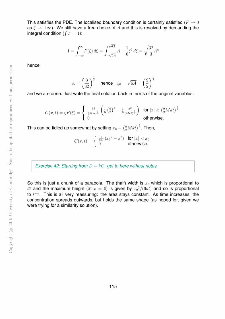
Cop
yri
ght
c ©20
19U
niv
ersi
tyof
Cam
bri
dge
.N
otto
be
quot
edor
repro
duce
dw
ithou
tp
erm
issi
on
This satisfies the PDE. The localised boundary condition is certainly satisfied (F → 0as ξ → ±∞). We still have a free choice of A and this is resolved by demanding theintegral condition (
∫F = 1):
1 =
∫ ∞−∞
F (ξ) dξ =
∫ √6A
−√
6A
A− 1
6ξ2 dξ =
√32
3A3
hence
A =
(3
32
) 13
hence ξ0 =√
6A =
(9
2
) 13
and we are done. Just write the final solution back in terms of the original variables:
C(x, t) = ηF (ξ) =
M
(Mkt)13
(16
(92
) 23 − 1
6x2
(Mkt)23
)for |x| <
(92Mkt
) 13
0 otherwise.
This can be tidied up somewhat by setting x0 =(
92Mkt
) 13 . Then,
C(x, t) =
{1
6kt(x0
2 − x2) for |x| < x0
0 otherwise.
Exercise 42: Starting from D = kC, get to here without notes.
So this is just a chunk of a parabola. The (half) width is x0 which is proportional tot13 and the maximum height (at x = 0) is given by x0
2/(6kt) and so is proportionalto t−
13 . This is all very reassuring: the area stays constant. As time increases, the
concentration spreads outwards, but holds the same shape (as hoped for, given wewere trying for a similarity solution).
115

Cop
yri
ght
c ©20
19U
niv
ersi
tyof
Cam
bri
dge
.N
otto
be
quot
edor
repro
duce
dw
ithou
tp
erm
issi
on
�
�
�(���)
This shows C(x, t) for successive timepoints, starting with red at t very small and thenmoving through the rainbow.
The sharp (or nearly sharp) edges might seem odd to start with, but recall the originalmodel: D = kC. So, our substance/population essentially cannot diffuse at very lowconcentration, so it piles up at the edge of its reaches, until there are enough to startmoving, explaining why this is such a weird boundary. This corner is a consequence ofour form of diffusion, together with condition that things are localised to the origin. end of
lecture 19
3.2 Travelling waves in reaction-diffusion systems
3.2.0 General F
From now on we focus on constant diffusivity D and work in one-dimension, unlessotherwise stated.
Recall the general transport equation had a term F (x, t) to represent the ‘creation/loss’of our stuff. So far we have looked at the behaviour of systems with diffusion, but theF has been restricted to just be linear growth of stuff i.e. F (x, t) = λC. In this section,we bring back the possibility of a more general F (C) (so local dynamics depends onconcentration of stuff, not time or space on its own), and we start to explore more theinteraction between local dynamics (F ) and spatial dynamics (diffusion terms).
∂C
∂t= D
∂2C
∂x2+ F (C)
116

Cop
yri
ght
c ©20
19U
niv
ersi
tyof
Cam
bri
dge
.N
otto
be
quot
edor
repro
duce
dw
ithou
tp
erm
issi
on
Another way to describe this is as a ‘reaction-diffusion’ equation: F is the reaction(change from non-spatial processes, or local processes) and obviously D ∂2C
∂x2is the
diffusion term.
This is, in general, a non-linear PDE in C (unless F happens to be proportional to C).First, see what happens if we revert to our usual tactic of solve and perturb. Thinkabout a purely spatially homogeneous dynamics first. Spatially homogeneous meansC(x, t) = C(t). Then subbing this in, our PDE becomes
dC
dt= F (C)
which is exactly the sort of thing we studied near the start of the course. Let us supposewe find C0 is a fixed point of this system, i.e. F (C0) = 0. Then consider a small spatialperturbation C(x, t) = C0 + ε(x, t). Subbing this in, we get a PDE for ε:
∂ε
∂t= D
∂2ε
∂x2+ F (C0 + ε(x, t)) ,
and as we take ε to be small, we can Taylor Series expand:
F (C0 + ε(x, t)) = F (C0)︸ ︷︷ ︸=0
+ε(x, t)F ′(C0)︸ ︷︷ ︸λ
+ O(ε2)︸ ︷︷ ︸neglect
and F (C0) = 0 as we were working around a fixed point. F ′(C0) is some number, call itλ. Ignore higher order terms. Then we have
∂ε
∂t= D
∂2ε
∂x2+ λ ε
which is exactly what we had near the end of subsection 3.1.2 when we consideredlinear growth. So we already know the outcome. If F ′(C0) < 0 then perturbationsabout C = C0 will decay and if F ′(C0) > 0 then perturbations will grow. Note that theseare also the same conditions for the non-spatial system, just classic section 1 styleresults.
What we ask next in this section is this: OK, we’ve done the linearised dynamics nearhomogeneous solution, what happens when the solution is further away from the equi-librium and the linear approximation isn’t valid? Can we get at the full dynamics inany way? This turns out to be rather tricky in general, but we will see some possibleapproaches below.
3.2.1 Fisher’s equation
We start by studying a classic equation, motivated by a classic model (first publishedin 1937 I think) which describes how a beneficial mutation can spread in a population.Imagine a spatial population and somewhere a mutation arises which turns out to begood for those individuals who carry that mutation. In population genetics, ‘good’ meanthey are fitter, which means they have more offspring.
117

Cop
yri
ght
c ©20
19U
niv
ersi
tyof
Cam
bri
dge
.N
otto
be
quot
edor
repro
duce
dw
ithou
tp
erm
issi
on
First we will build the model in a non-spatial setting. Let N(t) be the total populationand let p(t) be the proportion of the population which currently has the ‘good’ mutation(N > 0, 0 ≤ p ≤ 1). Suppose that at time t the non-mutant population is growing atrate λ and the mutant population at rate λ+ s. So s > 0 is the boost to the growth rateconferred by the mutation. Once the mutation has first appeared, there is no furthermutations happening, i.e. mutants give birth to mutants and non-mutants give birth tonon-mutants only.
Now build a picture of how things change in some short time δt (a bit like an approachyou may have seen to derive the rocket equation in Ia Dynamics & Relativity). Just forclarity in the table and below, write N = N(t) and p = p(t).
Number of Number oftime non-mutants mutants
(growth rate λ) (growth rate λ+ s)t N (1− p) Np
t+ δt N (1− p) (1 + λ δt) +O(δt2) Np (1 + (λ+ s)δt) +O(δt2)
To find N(t+ δt), add the number of non-mutants and mutants at time t+ δt:
N(t+ δt) = N(1− p)(1 + λ δt) +Np (1 + (λ+ s)δt) +O(δt2)
= N(1 + λ δt+ sp δt) +O(δt2)
And similarly to find p(t+ δt), divide number of mutants at time t+ δt by N(t+ δt):
p(t+ δt) =mutants(t+ δt)
N(t+ δt)=N(1− p)(1 + λ δt)
N(1 + λ δt+ sp δt)+O(δt2)
= p
[1 +
(s− sp)δt1 + (λ+ sp)δt
]+O(δt2)
= p [1 + s(1− p)δt] +O(δt2)
Hence (now writing p(t) properly) we have
p(t+ δt) = p(t) + sp(t) (1− p(t)) δt+O(δt2) .
So as usual, rearrange, take limit t→ 0 to get a differential equation for p:
dp
dt= sp(1− p)
and we recognise this as the logistic equation, again. This is maybe not a massivesurprise: a beneficial mutation, once introduced, should take over. In other words, pshould grow from small but positive up towards 1.
118
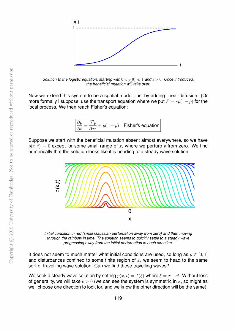
Cop
yri
ght
c ©20
19U
niv
ersi
tyof
Cam
bri
dge
.N
otto
be
quot
edor
repro
duce
dw
ithou
tp
erm
issi
on
�
�
�(�)
Solution to the logistic equation, starting with 0 < p(0)� 1 and s > 0. Once introduced,the beneficial mutation will take over.
Now we extend this system to be a spatial model, just by adding linear diffusion. (Ormore formally I suppose, use the transport equation where we put F = sp(1−p) for thelocal process. We then reach Fisher’s equation:
∂p
∂t=∂2p
∂x2+ p(1− p) Fisher’s equation
Suppose we start with the beneficial mutation absent almost everywhere, so we havep(x, t) = 0 except for some small range of x, where we perturb p from zero. We findnumerically that the solution looks like it is heading to a steady wave solution:
�
�
�(���)
Initial condition in red (small Gaussian perturbation away from zero) and then movingthrough the rainbow in time. The solution seems to quickly settle to a steady wave
progressing away from the initial perturbation in each direction.
It does not seem to much matter what initial conditions are used, so long as p ∈ [0, 1]and disturbances confined to some finite region of x, we seem to head to the samesort of travelling wave solution. Can we find these travelling waves?
We seek a steady wave solution by setting p(x, t) = f(ξ) where ξ = x− ct. Without lossof generality, we will take c > 0 (we can see the system is symmetric in x, so might aswell choose one direction to look for, and we know the other direction will be the same).
119

Cop
yri
ght
c ©20
19U
niv
ersi
tyof
Cam
bri
dge
.N
otto
be
quot
edor
repro
duce
dw
ithou
tp
erm
issi
on
Note carefully that at this point, we are just trying some constant c: we have no guar-antee that this will work for this c, or indeed for any value of c. In addition, suppose wefind some solutions, we don’t immediately know from this which travelling wave solutionit is that our general initial condition seems to be headed to. Still, the simulations areenough that this looks like it should work, so we carry on in hope.
Substituting this form into Fisher’s equation, we get a differential equation for f :
−cf ′ = f ′′ + f(1− f) .
There’s more than one way to proceed now, and we look at three apparently-differentapproaches in this course:
Approach 1 to Fisher’s equation: phase-plane analysis Essentially, we are look-ing for a solution to the DE for f that runs from near f = 1 to near f = 0. We couldthink of the second order DE as a coupled first order dynamical system for (f, f ′), anduse all of our usual tools to analyse it. Set f ′ = g, then:
f ′ = g
g′ = −cg − f(1− f)
Exercise 43:
• Check fixed points are at (0, 0) and (1, 0)
• Find the Jacobian at each of the fixed points
• Show that (1, 0) is a saddle (for c > 0)
• Show that (0, 0) is a stable node for c ≥ 2 and a stable focus for c < 2
(A stable node has both eigenvalues real and negative, and stable focus has acomplex conjugate pair of eigenvalues both with negative real part.)
The nullclines are straightforward: f ′ = 0 corresponds g = 0, i.e. the x-axis. And g′ = 0gives g = −c−1f(1 − f) which is the parabola in dashed blue in the diagrams below.Using the results of the fixed point types together with a nullcline analysis, it is not toohard to draw the phase-diagram53. Below we will consider c = 1, 2 and 3 and considerthe corresponding solutions that join (1, 0) with (0, 0). These trajectories between thefixed points correspond with solutions for f which run from near constant f = 1 tof = 0, as we want.
53and it’s even easier if you use mathematica...
120

Cop
yri
ght
c ©20
19U
niv
ersi
tyof
Cam
bri
dge
.N
otto
be
quot
edor
repro
duce
dw
ithou
tp
erm
issi
on
-0.2 0.2 0.4 0.6 0.8 1.0 1.2f
-0.3
-0.2
-0.1
0.1
g
5 10 15 20 25Ξ
0.2
0.4
0.6
0.8
1.0
fHΞL
This is c = 1. These do correspond to valid solutions of the Fisher equation, but as it goesinto f < 0, they can’t correspond to the travelling wave solution that we were looking for.
-0.2 0.2 0.4 0.6 0.8 1.0 1.2f
-0.20
-0.15
-0.10
-0.05
0.05
0.10
g
10 15 20 25 30Ξ
0.2
0.4
0.6
0.8
1.0
fHΞL
This is c = 2. This turns out to be the one we are after. The origin is a stable node.
121

Cop
yri
ght
c ©20
19U
niv
ersi
tyof
Cam
bri
dge
.N
otto
be
quot
edor
repro
duce
dw
ithou
tp
erm
issi
on
-0.2 0.2 0.4 0.6 0.8 1.0 1.2f
-0.15
-0.10
-0.05
0.05
0.10
g
15 20 25 30 35Ξ
0.2
0.4
0.6
0.8
1.0
fHΞL
This is c = 3. These also correspond to valid solutions of the Fisher equation, and are inright range, but turn out to not be the solution that we head to for general initial conditions.Note that the red trajectory is near the nullcline, but not exactly on it (this was where I had
problems drawing in lectures)
So with all this we can see that for each c > 0, there exists a corresponding steadywave solution. If we want f ∈ [0, 1] for all of x, then we can rule out the oscillatorysolutions (as f < 0 for some x). That just leaves us with all of c ≥ 2 to consider.
Approach 2 to Fisher’s equation: linearise near the leading edge Still thinking ofa wave moving to the right, we have f ≈ 0 for large positive ξ. So the dynamics outthere ought to be close to that of a system linearised around f = 0. Linearising justmeans ejecting the f 2 term here:
−cf ′ = f ′′ + f(1− AAf) .
i.e.f ′′ + cf ′ + f = 0
This is just a linear second order system with constant coefficients, so we can go aheadand solve with54 f = e−λξ for some λ and sub in:
λ2 − cλ+ 1 = 0
Normally we would now solve for λ (two solutions) and write down the complimentaryfunction and so on, but it all depends on c, so really focus on the relationship betweenλ (which determines the shape of the solution) and c (the speed):
54note minus in exponent, just so that we want real positive λ to have solutions that decay exponentiallytowards zero for large ξ.
122

Cop
yri
ght
c ©20
19U
niv
ersi
tyof
Cam
bri
dge
.N
otto
be
quot
edor
repro
duce
dw
ithou
tp
erm
issi
on
� � � � � ��
�
�
�
�
�
�
λ
�
Wave speed c as a function of the exponent of the shape of the wave λ. The red dot at(1,2) marks the minimum.
end oflecture 20
We can see that for real positive λ, we have c takes values in [2,∞).
Thinking back to the original system we have the Fisher equation in p
∂p
∂t=∂2p
∂x2+ p
has solution p = e−λ(x−ct) if c = λ + 1/λ. We have yet to say why the system settlesto one particular such speed and shape. Here, treat this next bit as starred, but solu-tions of the full nonlinear system will settle to the slowest wave speed of the linearisedsystem. Here is a sketch argument for this, but treat as starred:
**Arguments for slowest linear speed First, the nonlinear system speed must beone of the linear speeds (consider the leading edge as above, if we have a steadynonlinear solution, its front must satisfy the linear system). Second, we will show thatany nonlinear speed must be slower or equal to any linear speed. Combining these,the nonlinear speed can only be the slowest linear speed.
This can be done more formally (see work of Kolmogorov and others. . . ) but here’san intuitive picture. Our initial conditions are ‘localised’ to some region, so we can sayat least that p(x, 0) = 0 for x > x0 for some x0. Everywhere, p(x, 0) ≤ 1. So, we cancertainly bound our initial condition above by a curve of the form p = Ae−λx by choosingA large enough55. Use this p as an initial condition for the linearised system. So nowwe’re running two separate systems:
p(x, t) solves∂p
∂t=∂2p
∂x2+ p− p2
55A = eλx0 will do: then p > 1 for x < x0 and p > 0 everywhere
123

Cop
yri
ght
c ©20
19U
niv
ersi
tyof
Cam
bri
dge
.N
otto
be
quot
edor
repro
duce
dw
ithou
tp
erm
issi
on
p(x, t) solves∂p
∂t=∂2p
∂x2+ p
And we have rigged it so that p(x, 0) < p(x, 0). Consider both p and p running forwardin time now, each according to their own systems. Can p push past p? No, surely no.The extra −p2 pulls the p down. And, even without that, the diffusion tend to pull anyprotrusions back. To be slightly more formal, consider g(x, t) = p(x, t) − p(x, t). Wehave g(x, 0) > 0 for all x.
∂
∂tg(x, t) =
∂p
∂t− ∂p
∂t
=
(∂2p
∂x2+ p
)−(∂2p
∂x2+ p− p2
)=
∂2g
∂x2+ g + p2
>∂2g
∂x2+ g
So the g system is just diffusion and growth but with an extra p2 growth, which is non-negative. So if g starts non-negative everywhere, it will remain non-negative for alltime.
So we have that p bounds p for all time. And p is just one of the nonlinear solutions(we could choose the λ and it will trundle along with the appropriate speed c(λ) fromabove). Whatever p does, it cannot get past that big rolling road-block of the linearsolution. Hence, if it settles to a wave form with constant wave speed, that speedcannot be faster than c(λ) = λ+ 1/λ. This all works for any λ > 0.
If we accept this minimum speed argument, we now know that if the Fisher equationsettles to a constant speed, it must have speed c = 2.
Approach 3 to Fisher’s equation: mechanical analogy Really, this is firmly intothe land of overkill with respect to the Fisher equation: we don’t learn anything wedon’t already know from the other two approaches. However, it is included here forcompletion as it turns out to be useful with other systems where the earlier approachesdon’t work so nicely.
The idea is to take our differential equation in f and reinterpret it as a mechanicalsystem. We take ξ to be ‘time’ and f to be position56.
f ′′︸︷︷︸acceleration
= −cf ′︸︷︷︸force from friction
−f(1− f)︸ ︷︷ ︸−V ′ =Force from potential V
and take mass to be one to avoid that hassle. The first force is some sort of resistanceto motion: proportional to speed and in opposite direction. The second force is from
56this is the confusing bit as we really want x to be space, but just think of this as a separate systemnow for a moment. More serious is that ξ as time will feel backwards.
124

Cop
yri
ght
c ©20
19U
niv
ersi
tyof
Cam
bri
dge
.N
otto
be
quot
edor
repro
duce
dw
ithou
tp
erm
issi
on
some potential V (f), so here we need V ′(f) = −f(1 − f) hence V (f) = 12f 2 − 1
3f 3.
Perhaps the easiest way to imagine a potential is as a wire where V (f) gives its heightas a function of its position f .
-��� ��� ��� ��� ���
-����
����
����
����
����
�
�(�)
V (f) = 12f
2 − 13f
3 . Think of a bead on a wire of this shape, with a bit of friction.
We are seeking a solution which goes from one to zero as time (ξ) increases. Imaginethe bead starts close to that maximum at f = 1 and then slides towards the minimumat f = 0. If friction coefficieint c is low (but not zero), it will overshoot and oscillatearound f = 0. If friction is large enough, there is no overshoot. We call this overdamp-ing/underdamping in mechanics language.
It would be entirely reasonable to guess at this point that critical damping is at c = 2,without bothering to do any further work in this system.
� �� �� �� ��-���
-���
���
���
���
���
���
���
ξ
�(ξ)
������������ ��� �������� (�<�)
� �� �� �� ��
���
���
���
���
���
���
ξ
�(ξ)
����������� ���� �������� (�>�)
Solving system with f(0) = 0.99 and c = 0.2 (left) and c = 3.5 (right)
When working with this analogy, it is useful to remember that stability will appear tobe the wrong way around. In the world of the bead, f = 1 is unstable and f = 0 isstable. In the world of the Fisher equation, it is the other way around. The explanationis simply that time is reversed: ξ = x − ct is ‘time’ in bead world, and we have takenc > 0.
125

Cop
yri
ght
c ©20
19U
niv
ersi
tyof
Cam
bri
dge
.N
otto
be
quot
edor
repro
duce
dw
ithou
tp
erm
issi
on
3.2.2 Bistable systems
For Fisher’s equation above, there was one unstable state (p = 0) and one stable state(p = 1). So maybe it was not too surprising that we would find a travelling wave solution.Thinking in terms of the beneficial mutation: it is not surprising that it will spread and fixeverywhere (aka mutant invasion?). It is less obvious what happens when there’s twostable states: will one will win out if we’re at one state for part of space, and the otherfor another part of space?
We call such a system bistable. We actually have a bistable system at the ready fromearlier in the course: in section one we studied competition models using the exampleof wolbachia and mosquitos. After rescaling and so on we had
x = x
[x0 −
y
x+ y− (x+ y)
]y = y
[y0 − (x+ y)
]
Where x represent uninfected mosquitos, y is infected mosquitos. We have that 0 <y0 < x0 < 1. We know there are two stable fixed points (x0, 0) and (0, y0) which repre-sent the situation when no mosquitos are infected and when they all are, respectively.
It turns out that we can turn this apparently two-dimensional system into a one dimen-sional system by working in terms of proportion57 of mosquitoes that are infected: setu = y/(x+ y).
If we compute u using quotient rule and substituting the above equations, we find thatthe dynamics of u depends only on u: any other x,y dependency disappears.
Exercise 44: Show thatu = −u(u− r)(u− 1)
where r = x0 − y0, so we know r ∈ (0, 1).
57We have a small problem at the origin, but that situation is that there are no mosquitoes of any kind,so the model is kind of pointless.
126

Cop
yri
ght
c ©20
19U
niv
ersi
tyof
Cam
bri
dge
.N
otto
be
quot
edor
repro
duce
dw
ithou
tp
erm
issi
on
���
��
�
�
�
�
�(�)
Left: the phase plane in x and y. Right: now u as a function of t.
Dyn Sys note: we’re only looking at one dimension now, but we can see from the phasediagram that things collapse fairly quickly to the unstable manifold of that saddle point,so this is not unreasonable. We also can know the basins of attraction of the two stablefixed points58: it’s just the line y = rx.
In fact, this is a nicely generic one-dimensional bistable system: just a cubic givingstable points at 0 and 1 and unstable at r ∈ (0, 1). We can extend this to a spatialsystem just by adding diffusion:
∂u
∂t= −u(u− r)(u− 1) +
∂2u
∂x2
And now what happens? Suppose we have initial conditions where we are mostlyat zero, but have a patch with u ≈ 1. This is like we introduce our mosquitos withwolbachia some patch. Will the patch spread outwards or will it shrink? Both 0 and 1are stable, so which one wins? Things close to 1 should push towards 1, and thingsclose to 0 should push towards 0. But, diffusion hates sharp corners: we’re not goingto end up with a sharp boundary of all wolbachia and no wolbachia, it must blur out.
It turns out to depend on r, and we can show this by using the techniques we developedabove to look for travelling waves, then the mechanics approach is nice here. So, seeka travelling wave solution:
u(x, t) = f(ξ) where ξ = x− ct
Sub this in:−cf ′ = f ′′ − f(f − r)(f − 1)
58I left this suitably vague in the hand-drawn figures in section 1, but actually they’re just straight lines,it turns out
127

Cop
yri
ght
c ©20
19U
niv
ersi
tyof
Cam
bri
dge
.N
otto
be
quot
edor
repro
duce
dw
ithou
tp
erm
issi
on
Rearrange to think of as a mechanical system:
f ′′︸︷︷︸accelleration
= −cf ′︸︷︷︸friction
+ f(f − r)(f − 1)︸ ︷︷ ︸−V ′(f)
where V (f) is the potential (e.g. height of bead on a wire). We want
−V ′(f) = f(f − r)(f − 1)
So integrate up (choose constant, it does not matter):
V (f) = −1
4f 4 +
1
3(1 + r)f 3 − 1
2rf 2
Now consider the shape of this potential. There are maxima at 0 and 1 (the two sta-ble fixed points of u) and a minimum as r (the unstable fixed point of u). But, whichmaximum is higher? It depends on r.
Compare the heights of the maxima:
V (0) = 0 , V (1) = −1
4+
1
3(1 + r)− 1
2r =
1
6
(1
2− r)
so it depends: if r < 12
then higher max is at f = 1 and if r > 12
it is at f = 0. (Note,come back to equal case later.)
� ��
�(�)� < ���
� ��
�(�)� > ���
Now imagine the dynamics of our bead sliding with friction. Take c > 0 so that thefriction resists motion. If we start almost stationary near the lower maximum, we clearlycannot slide to the higher maximum. If we start near the higher maximum, then it ispossible59 that we go to the lower max exactly. If friction is too high, we fall short andend up in the minimum. If friction is too low, we will overshoot. So, there is one magicvalue of c in between where we grind to a halt exactly at the lower maximum.
59almost like when sports commentators call something a ‘theoretical possibility’: it is a possibility, justnot one we think is it all likely. However, here we are specifically hunting for the special outcome of goingfrom one of 0 and 1 to the other, not the typical dynamics.
128

Cop
yri
ght
c ©20
19U
niv
ersi
tyof
Cam
bri
dge
.N
otto
be
quot
edor
repro
duce
dw
ithou
tp
erm
issi
on
That will give a curve for f(ξ) which goes from 0 to 1 or vice versa. We do not reallymuch care about the shape of this curve, we just want to know which one can happen.Translate back to u(x, t) and we have the wave shape that moves to the right (with thespecial value of c).
�
�(���)
� < ���
�
�(���)
� > ���
Once the wave has passed through a region, it leaves u = 1 for r < 1/2 and u = 0for r > 1/2. So, if we want wolbachia to take hold in a population, we certainly needr < 1/2.
As a bonus, work this back to the original variables to see if it makes sense. We hadr = x0 − y0 were x0 and y0 were the carrying capacities of uninfected and infectedmosquito populations alone. Then, to say r < 1/2 is to say y0 > x0 − 1/2. In otherwords, having wolbachia does not reduce the carrying capacity of the population toomuch.
We know r < 1/2 is necessary for a successful introduction of wolbachia. Is it suffi-cient? Turns out no, not enough in bistable case. If the initial conditions are such thatthe initial introduction is too small or too narrow, it will not become established.
�
�(���)
�
�(���)
�
�(���)
129

Cop
yri
ght
c ©20
19U
niv
ersi
tyof
Cam
bri
dge
.N
otto
be
quot
edor
repro
duce
dw
ithou
tp
erm
issi
on
Here are three realisations with same system (r=0.3) and differing initial conditions. Theinitial conditions are in red (the blocky shape) and subsequent time points go through the
rainbow.
�
�(���)
�
�(���)
�
�(���)
In the top run, the initial window is toonarrow: diffusion of nearby uninfected
mosquitos will pull that initial spikedown.
In the middle run, the window ofintroduction is just wide enough, and
you can see several curves closetogether as the distribution hangs onthe brink of collapse, but it just gets
through, then settles to steadytravelling wave each way.
In the bottom run, the initial window isvery wide, and the solution quicklyreshapes to be the travelling wave
each way.
Exercise 45: Suppose insecticide kills mosquitos at some constant per capitarate (and it is the same for both infected and uninfected mosquitos). How willthis chance the required introduction width?
end oflecture 21
3.3 Spatial instabilities
So far in this section, we have had one variable at a time (concentration of bacteria,proportion of mutants, infected mosquitos). Here, we now extend to two variables.This is not just a more complicated version of the above, but it turns out that with twoquantities, we have some rather interesting new outcomes.
3.3.1 Chemotaxis
Chemotaxis sounds like something scary, but it just means the movement of somethingin response to a chemical. Here, think of small organisms (bacteria or amoebas, say)which more around slightly randomly, but generally prefer to go up (or down) the gradi-ent of the chemical. If go up the gradient, then we call the chemical a chemoattractant(it is like the bacteria are looking for the highest concentration, as they are attractedby the chemical). The chemical could be some nutrients that the bacteria are hunting.
130

Cop
yri
ght
c ©20
19U
niv
ersi
tyof
Cam
bri
dge
.N
otto
be
quot
edor
repro
duce
dw
ithou
tp
erm
issi
on
Or perhaps the chemical were excreted by the organisms themselves. For example, ifamoebas excrete a chemical and are also attracted by it, they should all end up cluster-ing. If they are repelled, then one might expect that to cause the population to spreadout.
Let us suppose we are dealing with a population of bacteria denoted by n(x, t) andsome chemical c(x, t). We can still use the transport equation for each of n and c. Wefinally use the active motion component, and say bacteria move speed v. There is stilldiffusion in there: think of this as a biased random walk60.
∂n
∂t+∇.(nv −Dn∇n) = F (n, c)
∂c
∂t+∇.( −Dc∇c) = G(n, c)
where Dn and Dc are the diffusion constants of the bacteria and chemical respectively.The right hand side (F and G) represent all the local dynamics: all the non-spatialprocesses, e.g more or less anything from section 1 of this course.
The active movement velocity v is for the chemotaxis. Let us take v = χ∇c, whichmeans if χ > 0 then the bacteria are swimming up the gradient of the chemical. Wecould in general have χ(c) so that the chemotaxis rate also depends on the chemicalconcentration, similar to the non-linear diffusion earlier, but here we will just take it tobe constant.
For the local dynamics:
F (n, c) = γ − δnG(n, c) = αn− βc
where all the constants (α, β, γ, δ) are positive. This represents a simple import (γ) anddeath (δ) model for the bacteria, and the chemical being excreted (α) by the bacteriaand decaying (β). So now our system is:
∂n
∂t+∇.(nχ∇c−Dn∇n) = γ − δn
∂c
∂t+∇.( −Dc∇c) = αn− βc
and note we have not actually specified what dimension of space we are working in,but it turns out below that this does not matter.
These tactics are the general to take with spatial systems:
• Deal with the spatially homogeneous system first60or think back to Fokker-Plank: there are analogous drift and spread terms here
131

Cop
yri
ght
c ©20
19U
niv
ersi
tyof
Cam
bri
dge
.N
otto
be
quot
edor
repro
duce
dw
ithou
tp
erm
issi
on
• Consider a small spatial perturbation around a fixed point
• Suppose the perturbation has the form cos(kx) (or cos(k.x) if more dimensions)
So working through for this example:
Spatially homogeneous first Here we treat everything as if it were constant inspace. We throw out the diffusion and chemotaxis term and set n(x, t) = n(t) andc(x, t) = c(t). Then we just have
n = γ − δnc = αn− βc
Solve for the fixed points, and find there is always one:
n∗ =γ
δ, c∗ =
αγ
βδ
Find the Jacobian at the fixed point:
J(n∗,c∗) =
(−δ 0α −β
)
The Jacobian as triangular, so we could just read off the eigenvalues and see they areboth negative so the fixed point is stable. For completeness though, note that the tracetr = −(δ + β) and determinant det = δβ. We will spot these again below in the spatialanalysis.
Consider spatial perturbations Start with a strategic rearrangement (put the diffu-sion and chemotaxis on the right):
∂n
∂t= γ − δn+Dn∇2n−∇.(nχ∇c)
∂c
∂t= αn− βc+Dc∇2c
Then perturb around the fixed point:
n(x, t) = n∗ + u(x, t)
c(x, t) = c∗ + v(x, t)
where both u and v are small, so we will linearise in these. The only tricky term is thechemotaxis one, but note that grad of a constant is zero so we lose ∇c∗ immediately.Also, we are linearising so throw out u∇v when it occurs in the chemotaxis term:
∇.(nχ∇c) = ∇.((n∗ + u)χ∇(c∗ + v)) = ∇.((n∗ + u)χ∇(v)) = ∇.((n∗)χ∇(v)) =γ
δχ∇2v
132

Cop
yri
ght
c ©20
19U
niv
ersi
tyof
Cam
bri
dge
.N
otto
be
quot
edor
repro
duce
dw
ithou
tp
erm
issi
on
so it is not so bad in the end. Continue subbing in our perturbation, linearising:
ut = −δu +Dn∇2u− γ
δχ∇2v
vt = αu− βv +Dc∇2v
We should consider taking general time initial conditions for u and v, but we couldconsider them as a sum of Fourier modes61. In fact, in this linear system we find thateach mode evolves on its own, so we can just consider a general mode.
If we are doing one-dimensional space, we could just look at perturbations with spatialform cos(kx). In general though, we could have vector k and x so we are looking atcos(k.x) and it will all work out the same. Some text books use eikx instead: I personallyprefer cos(kx), which makes it easier to think about the nature of the perturbation interms of bacteria and chemicals, but it is all mathematically equivalent, so feel free touse whichever you like. Whichever approach, the key thing is that ∇2 becomes −k2 (orperhaps we should say −|k|2 for the vectors).
Setu(x, t) = u(t) cos kx , then ∇2u = −k2u cos kx
and similarlyv(x, t) = v(t) cos kx , then ∇2v = −k2v cos kx
Substitute these in, cancel the cos kx everywhere, then our spatial system with pertur-bation of the form cos kx has become
ut = −δu −k2Dnu+ k2χγ
δv
vt = αu− βv −k2Dcv
There are lots of approaches continuing on from here, but I think the simplest is to reuseas much of our existing machinery as possible. We can read off the coefficients here toget a modified Jacobian: some terms are as before, and some appear with the spatialprocess. Say Jmod is the Jacobian in the u v system (i.e. under cos kx perturbation).Writing it strategically
Jmod =
(−δ 0α −β
)︸ ︷︷ ︸
Local dynamics
−k2
(Dn 00 Dc
)︸ ︷︷ ︸
Diffusion
+k2
(0 χγ
δ
0 0
)︸ ︷︷ ︸
Chemotaxis
The local dynamics are represented by the old Jacobian (which is exactly as we anal-ysed above when considering the homogenous system). The diffusion is −k2 timesa diagonal matrix, where the entries are the diffusion constants. The chemotaxis isrepresented also by a matrix with k2 factor, and here is a single off diagonal entry (thebacteria are undergoing chemotaxis due to the chemical).
61if this is confusing, look back at your Ib Methods notes: superposition of solutions, completeness ofeigenfunctions and so on, or just go with the flow here.
133

Cop
yri
ght
c ©20
19U
niv
ersi
tyof
Cam
bri
dge
.N
otto
be
quot
edor
repro
duce
dw
ithou
tp
erm
issi
on
As usual, we check for stability: it is stable if trace is negative and determinant ispositive. We already know that without the spatial components (which we can see isk = 0) then indeed these conditions are met. With the spatial components, the traceonly becomes even more negative
Tr(Jmod) = −(δ + β)︸ ︷︷ ︸Tr(J)<0
−k2(Dn +Dc) < 0
So, it comes down then to the determinant. If that is positive for a particular value of k,then the system is stable for that k. If it is positive for all (real) values of k, then we cansay the system is stable to small spatial perturbations of any kind. If the determinant isnegative for any k, then we have a spatial instability. So, let us go ahead and investigatethe determinant, remembering that we’re interesting in what happens for the full realrange of k (wlog k > 0).
Det(Jmod) =
∣∣∣∣( −δ − k2Dn k2 χγδ
α −β − k2Dc
)∣∣∣∣= (k2Dn + δ)(k2Dc + β)− k2χ
αγ
δ
= DnDc︸ ︷︷ ︸diffusions
k4 +(δDc + βDn − χ
αγ
δ
)︸ ︷︷ ︸
interactions between local and spatial
k2 + δβ︸︷︷︸old det
and so we have a quadratic in k2. The coefficient of k4 is the product of the diffusioncoefficients, and so is positive. The constant is the old determinant. This should notbe a surprise: if k = 0, then perturbing with spatial form cos kx is just the same as oldhomogeneous perturbation (old trace is also recovered above). We were working witha fixed point that is stable to homogeneous perturbations, so this det is positive. Themiddle term (coefficient of k2) is the fun one. Recognising the parameters, we can seeeach term is a product of local (α, β and δ) and spatial (Dn, Dc and χ) parameters.
Can this Det(Jmod) be negative for some real k? Well, yes. Just make the chemotaxiscoefficient χ big enough and Det goes negative and hence we have an instability forthat k. We can rearrange to get a condition for negative det (easier to reverse to secondto last line and rearrange for χ:
αγ
δχ >
(k2Dn + δ)(k2Dc + β)
k2
���
��
���
If we imagine starting with χ small, then there is no real k for which there is instability.If we increase χ, the first kc that goes unstable is the minimum of the RHS. We call
134

Cop
yri
ght
c ©20
19U
niv
ersi
tyof
Cam
bri
dge
.N
otto
be
quot
edor
repro
duce
dw
ithou
tp
erm
issi
on
this the critical wavenumber : the value of k when the instability first appears. With ageneral perturbation, it is this mode (cos kx) that will grow first.
Exercise 46: Show that we will have instability for χ > δαγ
(√δDc +
√βDn
)2.Find kc and check its dimensions.
end oflecture 22Think back to the original system: bacteria excrete chemical and also head up the
chemical gradient by chemotaxis. It’s hardly a surprise that it is unstable if there isenough chemotaxis: the bacteria are going to head to cluster together by calling toeach other with the chemical. It is fairly interesting though that the instability is first atan intermediate value of k (i.e. not k very small or very large), and we will see more ofthis below.
The fact that there is instability here is down to the chemotaxis. If χ = 0 there is nospatial instability. So, how about in general without chemotaxis? Consider generalreaction-diffusion systems. Suppose we have some system where the local dynam-ics is stable (around some fixed point). If the only spatial process is diffusion, thenalone is also going to support stable dynamics as it just smoothes stuff out. Can thecombination cause an instability?
In one dimension, we already know the answer. In section 3.1.2 we had a diffusionequation with linear growth, and found that the growth term is beaten by the diffusivespread in an infinite domain. In 3.2.0 we found that a more general local term stillbehaves like a linear term for small perturbations, so nothing much changes. So in onedimension, there’s no possibility of a spatial instability if the local dynamics are stableand all we have is diffusion.
In two or more dimensions, well, read on. . .
3.3.2 Turing instabilities
We will now see that in two (or more) dimensions, it is possible to have a spatial insta-bility in a system which is stable to homogenous diffusion and the only spatial processis linear diffusion. This result was first shown in a paper by Alan Turing published in1952. This result is not just mathematically interesting, but also is exciting as it givesa mechanism for patterns to emerge from a homogenous system. This is important indevelopmental biology: how do things grow? For anything from coat patterns (spotsand stripes) to anatomy of any growing creature, there must be some mechanism tocreate spatial structure starting from something uniform. The beautiful thing is that wedo not need to write down some extremely complicated system, but we can set it upfrom two chemicals (morphogens here) in the type of mathematical language we haveused above.
So, to the general theory: start with two chemical concentrations, u and v, which areboth functions of space and time, and write down a general system where they have
135
Cop
yri
ght
c ©20
19U
niv
ersi
tyof
Cam
bri
dge
.N
otto
be
quot
edor
repro
duce
dw
ithou
tp
erm
issi
on
some local dynamics (given by functions f and g) and their spatial dynamics are justlinear diffusion (with rates D1 and D2):
∂u
∂t= f(u, v) +D1∇2u
∂v
∂t= g(u, v) +D2∇2v .
We will first analyse the homogenous system and suppose we find a stable fixed point,then we look at what happens to spatial perturbations about this fixed point. In otherwords, this tracks through much as the chemotaxis example above, but we work with ageneral system here with just diffusion.
First, the homogenous system then. Formally, this is considering the case where uand v are constant in space but may vary in time, so we are setting u(x, t) = u(t) andv(x, t) = v(t). More simply in practice, just cross out the diffusion terms and we’reback to Section 1. We are seeking fixed points, i.e. we want u∗ and v∗ such thatf(u∗, v∗) = g(u∗, v∗) = 0. In particular, we want stable fixed points. We write theJacobian at this fixed point as:
J =
(fu fvgu gv
)where this is slightly lazy notation as we really mean these all evaluated at the fixedpoint, i.e.
fu =∂f
∂u
∣∣∣∣(u∗,v∗)
, fv =∂f
∂v
∣∣∣∣(u∗,v∗)
etc. .
For a Turing instability, we want the homogenous system to be stable (otherwise it’srather boring). So we require:
Tr(J) = fu + gv < 0
Det(J) = fugv − fvgu > 0
for stability. For given functions f and g, this usually boils down to some nice parameterrange. So now suppose that we have a fixed point, and that we are in the parameterrange where it is stable from now on.
Now, consider spatial perturbations about this homogenous fixed point of this form:
u(x, t) = u∗ + u(t) cos kx
v(x, t) = v∗ + v(t) cos kx
where u and v are functions of time (but not space) and we are interested in the dy-namics when they are small. So, speeding through this (as it goes much like the
136

Cop
yri
ght
c ©20
19U
niv
ersi
tyof
Cam
bri
dge
.N
otto
be
quot
edor
repro
duce
dw
ithou
tp
erm
issi
on
chemotaxis example above), we know that the cos will cancel everywhere. This will justleave a factor −k2 with the diffusion, so to linear order we have:
u′ = fuu+ fvv − k2D1u
v′ = guu+ gvv − k2D2v
where prime denotes differentiation wrt t. Hence, reusing the notation of the modifiedJacobian, we can read off:
Jmod =
(fu fvgu gv
)︸ ︷︷ ︸
original J
− k2
(D1 00 D2
)︸ ︷︷ ︸
from diffusion
.
To see if the spatial perturbation is stable or unstable, we can now just work with thismodified Jacobian. Calculate the trace and det, and try to pull out terms which are thetrace and det from the original Jacobian:
Tr(Jmod) = (fu + gv)︸ ︷︷ ︸old Tr
−k2(D1 +D2)
and as the trace of the homogenous J was negative (as we decided we were going tolook at stable fixed points only) this trace of Jmod is certainly negative. So, that’s dealtwith.
The real fun begins with the determinant:
Det(Jmod) = D1D2︸ ︷︷ ︸>0
k4 − (D1gv +D2fu)︸ ︷︷ ︸the magic!
k2 + (fugv − fvgu)︸ ︷︷ ︸old Det
Looking at this as a quadratic in k2, there are three terms. The coefficient of k4 is justthe product of the diffusion coefficients, so this is always positive. At the other end,the term which is constant in k is just the original determinant. This is not a surpriseas k = 0 just recovers the the original Jacobian. The term in between is the reallyinteresting one. Notice the k4 term contains just constants from diffusion, nothing fromthe local dynamics. The constant term is the other way: just the local dynamics, andnothing from the diffusion process. The term in the middle somehow represents theinteraction between the diffusion and the local dynamics: there are both D1,D2 and f ,gin there.
Is this perturbation stable? It is if both the trace is negative (which it is) and the det ispositive (which is in question). So, is it possible that det < 0 for some value of k (orsome range of values of k)?
Rewrite as follows62:Det(Jmod) = Ak4 −Bk2 + C
62Note the minus sign before B. Can do it either way, but this makes more sense to me in the end.
137

Cop
yri
ght
c ©20
19U
niv
ersi
tyof
Cam
bri
dge
.N
otto
be
quot
edor
repro
duce
dw
ithou
tp
erm
issi
on
where we have already that A, C are positive. For this to be negative, we certainly needB > 0 (sometimes this is referred to as the ‘necessary’ condition). Suppose that is truefor now. Think about this graphically, plotting determinant against k2. It is a parabola,with a minimum at k2 = B/2 which is positive. We can now see that it depends whetherthe minimum is above or below zero:
��
�
���
Parabolae with A,B,C > 0: one in blue does not have any real roots and never negative(in real k2). One in gold has real roots, so there is a range of k2 > 0 which where Det < 0.
In fact, within B > 0 we can now see we also need there to be real roots63 for Det < 0in some range of (real) k, hence we need positive discriminant: B2 − 4AC > 0.
Pulling this together, we have spatial instability for some k iff
B > 0 AND B2 − 4AC > 0
(and this pair of conditions together are now necessary and sufficient). Of course, aswe know the signs of A and C we can get this down to being equivalent to a singlecondition:
B > 2√AC .
This might look simpler, but sometimes in a given example it is easier to use the twoconditions.
Putting back in the full expressions for A, B and C we can then write down a conditionin full:
D1gv +D2fu > 2√D1D2(fu gv − fv gu)
condition for Turing Instability
63Plural if we’re being careful: equal roots just means it touches Det = 0, but we actually need itnegative to be sure of instability so use strict inequalities here.
138

Cop
yri
ght
c ©20
19U
niv
ersi
tyof
Cam
bri
dge
.N
otto
be
quot
edor
repro
duce
dw
ithou
tp
erm
issi
on
This is a nice core result here. However, please do not put any effort into memorisingthe expression here: the condition for a given example can usually be derived moredirectly than plugging things into here.
Imagine now that there is some parameter (within f or g) that we are varying, and forsome range this condition is not met, and for some other range, it is met. The transitionas we move between them is for no instability to having instability for some range ofk. The value of k that first is unstable as we transition is the critical wave number, kc.Algebraically, it is when our quadratic in k2 has a double root. In other words the doubleroot of Ak4 − Bk2 + C = 0 in the case when B2 − 4AC = 0. One can write this valuedown in many ways e.g.
k2c =
√C
Aor k2
c =B
2A
and they will all be equivalent so just choose whichever one is convenient. It is usuallypossible to eliminate one parameter.
Finally, we can think about Turing Instabilities in a few different ways to try to build moreintuition about what they are and how they occur:
Thinking about wavelength Our perturbation was of the form cos kx so the wave-length is 2π/k.
• If k � 1: these are really long waves. On the scale that diffusion operates on,these look to be almost constant. So diffusion does not do very much, and hencethe dynamics are approximately the local dynamics alone. Indeed, we can checkabove and see that for small k, Jmod ≈ J . And in our quadratic for the determinant,it is indeed approximately the old determinant. If we have conditioned on the localdynamics being stable, then we should not find instability for k � 1.
• If k � 1: these are really short waves, with wiggles with high curvature. Diffusionis fast to eliminate wiggles, so in this range expect diffusion to dominate, andhence things to be stable, no matter the local dynamics.
Hence we can start to understand why instability can only occur for some intermediaterange of k. Either regime of diffusion or local dynamics dominating will result in stability.The only possibility is somewhere in between.
Thinking about the algebra This is a nice way to grasp why we really have to have asystem of two or more dimensions (u and v) and to discover that we must have differingdiffusion rates. We can see in general that in general our modified Jacobian will be theold Jacobian minus k2 times some diagonal matrix with positive elements:
Jmod = J − k2D
where D is a matrix with D1, D2 etc down the diagonal.
139

Cop
yri
ght
c ©20
19U
niv
ersi
tyof
Cam
bri
dge
.N
otto
be
quot
edor
repro
duce
dw
ithou
tp
erm
issi
on
For a Turing instability, we want the local dynamics to be stable, but not the spatialdynamics (for some values of k) – indeed perhaps this is the definition of a Turinginstability. In terms of matrices then, we want all eigenvalues of J to have negative realpart, but not true for Jmod.
Brief aside: If a matrix M has eigenvector v with eigenvalue λ, then matrix M − µI(where I is the identity matrix) has the same eigenvector but now the eigenvalue isλ− µ.64
So if the diagonal matrix D was in fact a multiple of I, then all of our new eigenvalueswould be the old ones minus some real positive number, and hence still stable. Hencewe cannot have D1 = D2 and still get a Turing instability. Or in more dimensions,we can’t have the diffusion coefficients all be equal. In one dimension? Well, it isconsistent: we really can’t have a Turing instability.
Back to two dimensions: might be confusing that Turing instabilities are possible at allnow. It still feels like subtracting stuff off the diagonal should make the eigenvalueshave more negative real part. Maybe this tends to be true more often than not, but itcertainly is possible to subtract things off the diagonal and grow the real part of one ofthe eigenvalues, which is all we need.
All of this is mainly to build intuition about what is going on here, but it is also slightlyuseful in practice: we often have D1 = 1 and D2 = d or similar. Then we know d = 1cannot be in the range where a Turing instability is possible. This often a useful sanitycheck in working through a particular example.
Activator-Inhibitor dynamics Turing instabilities are often introduced which the mech-anistic explanation being in terms of ‘activator-inhibitor’ dynamics. Think of u and vas being some chemicals and here one is an ‘activator’ so its presence generally in-creases one/both of them and the other decreases one/both. This doesn’t work per-fectly for all examples, but it is still a useful way to think about it sometimes. We canconnect it with the algebra above:
B > 0 corresponds to D2fu +D1gv > 0
Tr < 0 corresponds to fu + gv < 0
So we have two different linear combinations of fu and gv with positive coefficients, andone combination is positive and the other is negative. So we must have exactly one offu and gv positive and one negative. Without loss of generality, say fu < 0 < gv andthen we would naturally think of f as an inhibitor: fu < 0 means that it dampens itselfback down (1-D dynamics on its own are stable). Similarly g is the activator. Looking atthe coefficients above, we can see in this case we need D1 > D2
65 Hence the inhibitor64Easy to check: (M − µI)v =Mv − µIv = λv − µv = (λ− µ)v.65Either stare at the two inequalities for a while, or do something more organised like consider
(D2fu +D1gv)︸ ︷︷ ︸>0
−D2 × (fu + gv)︸ ︷︷ ︸<0
= (D1 −D2)gv.
140

Cop
yri
ght
c ©20
19U
niv
ersi
tyof
Cam
bri
dge
.N
otto
be
quot
edor
repro
duce
dw
ithou
tp
erm
issi
on
diffuses more than the activator. We also must have |gv| < |fu| in this case, so theinhibitor is ‘stronger’ in some sense.
This can make intuitive sense: the activator works very locally to stimulate the pertur-bation. The inhibitor spreads out and pushes things a bit further away in the oppositedirection. So if the perturbation is flat, it gets pushed back. If the perturbation is wavywith about the right wavelength, then it may grow.
This is useful for building intuition as it helps underline why there must be (at least) twoquantities. It also shows in another way that Turing instabilities are about how the localdynamics interact with diffusion in just the right way at approximately the right wave-lengths. But, be cautious not to push this too far: for setting up which is the activatorand which is the inhibitor, we have not thought about how the two quantities interactwith each other (which are encapsulated, at least to first order, by fv and gu). end of
lecture 22
Worked example: Finally to finish this section, and the course, here is an examplequestion on Turing instabilities:
Consider this system:
∂u
∂t= −u+ u2v +∇2u
∂v
∂t= b− u2v + d∇2v .
Find condition for this system to have a Turing instability. Find the critical wavenum-ber kc on the boundary of instability.
To illustrate to tackle these problems in practice, the solution (with annotation in red) isin my handwriting on the remaining pages.
141

Cop
yri
ght
c ©20
19U
niv
ersi
tyof
Cam
bri
dge
.N
otto
be
quot
edor
repro
duce
dw
ithou
tp
erm
issi
on
142

Cop
yri
ght
c ©20
19U
niv
ersi
tyof
Cam
bri
dge
.N
otto
be
quot
edor
repro
duce
dw
ithou
tp
erm
issi
on
143