1

PART II - LOCALIZED AND COMPARATIVE STUDIES

PARTE II - ESTUDIOS LOCALIZADOS Y COMPARATIVOS

OCEAN SCALE AND REGIONAL COMPARISON - ESTUDIOS

OCEANICOS Y COMPARACION REGIONAL

INFLUENCE OF THE OCEAN ON THE ATMOSPHERIC GLOBAL

CIRCULATIONS AND SHORT-RANGE CLIMATIC FLUCTUATIONS

by

Tatsushi Tokioka

Meteorological Research Institute Nagamine 1–1, Tsukuba, Ibaraki 305

Japan

Resumen

Alrededor del 70% de la superficie de la tierra está cubierta por los océanos. Se reconoce que los intercambios de energía y momentum entre la atmósfera y el océano son muy importantes para mantener la circulación global de la atmósfera. Otro aspecto importante del océano es su amplia inercia térmica comparada con la de la atmósfera y la superficie de la tierra. La anomalía térmica observada en la parte superior del océano tiene un tiempo de persistencia de varios meses lo que es casi un orden de magnitud mayor que las anomalías dentro de la atmósfera. Por esta razón, se considera que la anomalía de la temperatura de la superficie del mar es uno de los frentes superficiales más importantes para los fines de predicción de corto alcance de las fluctuaciones climáticas.

Han habido estudios muy activos donde se han descubierto relaciones entre las anomalías de la temperatura de la superficie del mar y la circulación anómala dentro de la atmósfera. Una de las variaciones no estacionales más notables observadas en la temperatura superficial del mar es aquella asociada con el fenómeno de El Niño. En la etapa madura de El Niño, la mitad oriental del océano Pacífico tropical tiene una temperatura superficial del mar que es mucho más cálida de lo normal. Al mismo tiempo la parte occidental del océano Pacífico subtropical está cubierto de una temperatura superficial del mar más fría que lo normal.

Durante el fenómeno de El Niño se observan fuertes lluvias en el área de anomalía cálida de la temperatura de la superficie del mar. Se presenta una liberación anómala del calor latente en la misma región, lo que causa cambios en las circulaciones este-oeste (circulación de Walker) en su ubicación e intensidad dentro de los trópicos. En las bajas latitudes también se observa una marcada anomalía de número de onda l en dirección este-oeste en la presión a nivel del mar. Esto coincide con el fenómeno que por mucho tiempo ha sido reconocido como Oscilación del Sur. Independientemente de la longitud, en la parte superior de la troposfera tropical se observan temperaturas más altas y una mayor altura geopotencial.

En base a las observaciones se ha establecido que durante el fenómeno de El Niño las anomalías de la circulación de la atmósfera se extienden hacia latitudes extratropicales en el invierno del

2

hemisferio norte. El mecanismo de teleconección puede ser explicado como una propagación de las ondas externas de Rossby dentro de la atmósfera.

Aparte del fenómeno del El Niño, también se han estudiado las conecciones entre otras anomalías de la temperatura superficial del mar y la circulación anómala de la atmósfera, y se han descubierto correlaciones significativas entre ellas en áreas y épocas particulares.

Varios investigadores han reportado estudios teóricos y numéricos relacionados con las anomalías de la temperatura superficial del mar. Estos investigadores están de acuerdo en que la anomalía de la temperatura superficial del mar a bajas latitudes tiene importancia en producir una respuesta significativa a través de la atmósfera global. Algunas conecciones encontradas en el fenómeno de El Niño han sido confirmadas por experimentos numéricos recientes usando el modelo global atmosférico.

Los estudios mencionados anteriormente nos proporcionan ejemplos de que los pronósticos mensuales y estacionales son factibles para áreas seleccionadas bajo circunstancias particulares, si es que las anomalías de la temperatura superficial del mar son conocidas con anterioridad. De momento, se considera que una forma muy directa de desarrollar un sistema de corto alcance para pronosticar el clima es mediante la extensión de modelos usados para la simulación de la circulación global atmosférica o por las predicciones del clima de corto o medio alcance, aun cuando algunas mejoras en el modelo pueden ser necesarias. Entre estas se incluyen las mejoras en la descripción de los fenómenos físicos en la superficie y los intercambios de temperatura turbulentos, la humedad y el momentum en la superficie.

INTRODUCTION

Ocean influences the atmospheric global circulations both thermally and dynamically. The source of energy that drives the atmospheric global circulations is the solar energy. This does not mean that the atmosphere receives energy directly from the sun. Actually, the earth's surface is the main absorber of the solar energy. Fig. 1 shows schematically how energy flows within the atmosphere. The incoming solar energy flux is normalized as 100. About 30 is returned back to space without being absorbed by the earth or the atmosphere, and 70 is absorbed by either of them. The figure shows that about 70% of the absorption takes place at the earth's surface, and that the energy is transferred from the earth's surface into the atmosphere through sensible and latent (water vapour) heat fluxes due to turbulent motions and through the terrestrial radiation. About 70% of the earth's surface is covered by the ocean, and the ocean absorbs the solar energy more efficiently than the land surface. In this sense, the ocean is a very important agent that determines the present climate.

3

Figure 1: A schematical figure to show energy flow within the earth's atmosphere. Incoming solar radiation (338 w/m2) is normalized as 100. All the energy fluxes are expressed in the normalized unit.

The major physical elements and feedback processes of the coupled atmosphere-ocean system is shown in Fig. 2. Evaporation (latent heat flux) from the ocean surface supplies water vapour to the atmosphere. Latent heat is transformed into sensible heat when condensation takes place, and water goes back to the surface. Usually the place of condensation differs from that of evaporation due to atmospheric motions. Therefore the place where the atmosphere is heated through condensation differs from the place where the surface loses its energy through evaporation. Both evaporation and condensation also cause salinity change, and thus density change, within the ocean.

4

Sensible heat flux through the ocean surface causes temperature change in both the atmosphere and the ocean. Because of the big difference in the thermal inertia between them, the temperature change in the sea surface temperature (SST) is usually small compared to that in the surface air. When the ocean surface is being heated, the shallow upper layer of the ocean is effectively heated due to the stable stratification, and the SST increases fairly rapidly. On the other hand, when the ocean surface is being cooled, downward convection takes place, mixing a relatively thick layer, and changing the SST only slightly.

Figure 2: The major physical elements and feedback process of the coupled atmosphere-ocean system. (Taken from Gates, W.L., 1976, Bull. Am. Meteorol. Soc., 57:542)

Global motions within the atmosphere are initiated by the non-uniform heating in the horizontal direction due mainly to geometry and non-uniform topography. The atmospheric global circulations thus initiated transport airmass, energy (or temperature), water vapour and momentum within the atmosphere. Oceanic circulations are initiated not only by the non-uniform density distribution in the horizontal direction caused by heating and salinity change but also by the wind stress at the ocean surface or the momentum transfer through the surface, and transports mass, energy and momentum within the ocean.

The transports of energy and momentum from the earth's surface to the atmosphere due to turbulent motions are given by the following empirical forms:

5

Fs, Fw and Fv are the sensible heat flux, the latent heat flux and the momentum flux vector respectively, : the density of the surface air, cD: the drag coefficient, |Vs|: the amplitude of the surface wind Vs , Ss : dry static energy (enthalpy + geopotential) of the surface air, Sg : dry static energy of the earth's surface, L: the latent heat of vaporization, qs : the mixing ratio of the surface air, q*

g : the saturation mixing ratio of the earth's surface, r: the factor which depends on the ground wetness. It is noted that no direct information about the oceanic surface currents enter in Eq.(3). This is because the intensity of the surface current of the ocean is much smaller than the atmospheric wind speed. Therefore, changes (or anomalies) in the ocean surface conditions are not recognized by the atmosphere through the dynamical link well, but through the thermal link. On the other hand, changes (or anomalies) in the atmosphere are recognized by the ocean through the dynamical link rather than through the thermal link. This is because the thermal relaxation time of the ocean is longer then the dynamical response time scale of it, due to the large thermal inertia of the ocean.

The changes in the atmospheric circulations are caused by many other processes, for example through interactions with the surface boundaries other than ocean (bare land, snow and ice), through changes in the atmospheric compositions which cause changes in the radiative heatings, such as CO2, aerosols and so on. These changes may further trigger changes in the oceanic circulations also.

In this paper, a brief summary will be given on the influence of the ocean on the mean atmospheric circulations, and on the observational links between the SST anomalies (SSTA) and the anomalous atmospheric circulations (AAC). Then some theoretical and numerical model studies concerning the influence of the SSTA on the AAC are reviewed. Whether those anomalies are predictable or not is a very important and also a very interesting problem. Present views on that problem will be given in a later section.

THE OCEAN'S ROLE IN THE MAINTENANCE OF CLIMATE

Ocean is distributed non-uniformly on the globe. Therefore geographical differences in the seasonal variations of the circulation may be viewed as a measure of oceanic influence on the seasonal cycle. For example, the annual amplitude of surface air temperature shown in Fig. 3 confirms the widely-held impression that the seasonal variations are much less over ocean than over land. This seasonal modulation by ocean is recognized also in other statistics of circulations, such as pressure, wind, precipitation and cloudiness.

Dynamically, the oceanic surface is smoother than the land surface. Therefore the wind speed can be larger near the oceanic surface than near the land surface, if other conditions are the same. The zonally averaged sea level pressure is shown in Fig. 4. for both January and July. One of the most notable features of the figure is a large pressure gradient in the north-south direction around 500S in both months. The latitude zone just coincides with the position of circum-antarctic oceanic belt, where the zonally averaged westerly wind at the surface is the strongest. The zonally averaged wind is approximately connected with the zonally averaged mass distribution through the following geostrophic wind balance:

6

Figure 3: The global distribution of annual amplitude of surface temperature (oK), with the solid line drawn every 40K. (Taken from Monin, A.S., 1976, “The physical basis of climate modelling,” GARP Pub. Ser. No 16).

Figure 4: The zonally averaged sea level pressure (mb) for January and July.

where [u] is the zonally averaged eastward wind, [p] : the zonally averaged air density, f : the Coriolis factor (=2 sin ), : the rotation rate of the earth, : latitude, a: the radius of the earth. Therefore we may explain the feature noted above as a dynamical effect of the ocean.

More quantitative study has been presented by Oort and Vonder Haar (1976), with respect to ocean's contribution to the total energy balance of the atmosphere-ocean system. They estimated the seasonal variation of the oceanic heat flux required in the northern hemisphere to maintain an overall balance in the system. The rate of heat storage in both the atmosphere and the ocean is determined based on observational data and is shown in Fig.5 (a) and (b), respectively. The rate of atmospheric heat storage reaches a maximum in May at high latitudes, while the oceanic heat

7

storage rate is a maximum in June in middle latitudes. Somewhat larger heat storage rate and a more complicated meridional and seasonal structure in the ocean are also noted, compared to that in the atmosphere. In mid-latitudes, the oceanic heat storage rate is approximately in phase with the net radiational heating rate and serves to reduce the seasonal contrast by storing heat in summer and releasing it in winter. While near 15°N, the ocean exhibits a maximum storage in spring and a minimum in fall. This behaviour is apparently related to seasonal variations of low-latitude upwelling.

Fig.6 (a) and (b) show the seasonal variation of the meridional heat flux in both the atmosphere and the ocean for the northern hemisphere. The flux in the ocean is obtained as a residual of the energy budget equation. A strong northward heat flux is found in winter in the atmosphere, while the oceanic heat flux exhibits a strong semi-annual variation, with maximum northward heat flux in spring and fall in the sub-tropics and southward flux in winter and summer in higher latitudes. In the tropics, an intense southward heat flux occurs in summer, contributing to reduce the global-scale latitudinal contrast of temperature. The amount of heat flux reaches as much as 8 × 1015 W during August, the maximum heat flux found in the atmosphere-ocean system. Although some errors may be inevitable in residuals, Oort and Vonder Haar clearly demonstrate that the ocean is at least as important as the atmosphere in satisfying the heat transport requirement of the atmosphere-ocean system.

Figure 5: Rate of heat storage (W/m2) in the atmosphere (a) and in the ocean (b). (Taken from Oort and Vonder Haar, 1976).

8

Figure 6: Northward flux of energy (1015W) in the atmosphere (a) and in the ocean (b). (Taken from Oort and Vonder Haar, 1976).

Figure 7: (a) SST deviations from the 1947–1966 man (dashed line) for the North Pacific in the region 15° to 60°N and 130°E to 110°W. Thin lines connect monthly anomalies; the thick curve shows the 12-month running means. (taken from Namias and Cayan, 1981).

(b) 12-month and (c) 36-month running means of the surface air temperature deviations averaged over the northern hemisphere (solid line). The two dotted curves represent the 95% confidence limit for the error. (Taken from Yamamoto and Hoshiai, 1979).

9

Figure 8: Cross-correlations of 700mb height (top) and sea level pressure (bottom) with the values at the point (40°N, 150°W) for winter. (Taken from Namias, 1982).

NON-SEASONAL CHANGES OF SST AND ATMOSPHERIC CIRCULATIONS

It may be convenient to group studies into four categories, i.e., changes in the hemispheric scale, the changes within the mid- and high-latitudes, the changes within the tropics and the teleconnection between the tropics and the extratropics.

The changes in the hemispheric scale

Namias and Cayan (1981) have shown the existence of interseasonal and interannual changes in the averaged SST departures from the 1947 – 1966 mean SST for the North Pacific in the region 15° to 60°N and 130°E to 110°W. The region corresponds to 20% of the hemisphere. In Fig.7(a) are shown monthly values and their 12-month running means. In the figure, the low frequency signal of the North Pacific SST is quite clear, having periods of several years. The largest anomaly within that period is almost as much as 0.5K over the bulk of the North Pacific.

Changes in the atmospheric temperature have been studied by many workers (Yamamoto et al.,1975; Angell and Korshover, 1977, 1978; Yamamoto and Hoshiai, 1979, etc.). They have shown the existence of interannual changes of atmospheric temperature globally as well as hemispherically. Fig.7 (b) and (c), obtained by Yamamoto and Hoshiai (1979), show 12-month and 36-month running means of the surface air temperature deviations over the northern hemisphere. It is interesting to note similar variations between (a) and (b) or (c). This indicates some connections between the SST in the North Pacific and the surface air temperature of the northern hemisphere. From further comparison of those figures, several months' delay, say 6 months, seems to be noted in the peaks of the surface air temperature anomalies.

10

Regional studies in the extratropics

Many studies have been reported on the behaviours of the SSTA (sea surface temperature anomaly) and of the AAC (anomalous atmospheric circulation) in the extratropics, especially in the North Pacific. Namias (1982) has shown that there is a great deal of spacial coherence in the SSTA, and that the overlying atmospheric anomalies of mid-tropospheric heights go with high (low) SST's and enhanced northerly air currents off the West Coast are associated with cold water, whereas high pressures and southerly current usually go with warm currents.

The coherence of SSTA over the North Pacific with respect to time is studied by Namias and Born (1970) and Walsh and Richman (1981). In Fig.9 are shown the lagged autocorrelations of monthly mean of SST, 700mb height and sea level pressure, which confirm the fact that SSTA's have their persistence time of several months, which is almost an order of magnitude longer than that of anomalies within the atmosphere. The seasonal dependence of the persistence of SSTA has also been clarified. Fig. 10 shows lagged autocorrelations of SSTA, based on the first five EOF (empirical orthogonal function) modes of SSTA, obtained for each season centered on January, April, July and October (Walsh and Richman, 1981). Notice that seasonal persistence is largest when winter (January) is antecedent, and that the persistence does not decrease monotonically with lag. Persistence from January actually increase monotonically with lag. Persistence from January actually increases between lags of 9 and 12 months. Namias and Born has suggested that the warm and shallow mixed layer formed in the upper part of ocean in summer might temporarily shield the SSTA, causing low correlations during that season. Relatively high correlation in the persistence from April between lags of 6 and 10 months may be due to the same mechanism.

Because of the persistent nature of the SSTA mentioned above, and because of sizable effects of the SSTA on the atmospheric global circulations, SSTA is considered as one of the most important predictors of monthly or seasonal predictions (or short-range climate prediction). Namias (1968, 1969, 1971, 1972) pioneered in this respect. Namias (1976) showed that the North Pacific SSTA in summer are significantly correlated with the sea level pressure in fall in the area of the Gulf of Alaska and the temperature anomaly in the United State. Davis (1978) indicated that autumn and winter sea level pressure (SLP) anomalies are predictable from prior observations of either SST or SLP over the North Pacific. On the other hand, he found little or no predictability in SLP of other seasons. Concerning the temperature forecast over the United States, many studies (Harnack and Landsberg, 1978; Harnack, 1979; Walsh and Richman, 1981; Barnett, 1981) followed after Namias (1976), showing that predictions of temperature anomaly over North America are feasible for particular seasons and areas, by use of the SSTA in the North Pacific. Highest predictability is shown in winter along the west coast, the southeastern United States, the northern tier of states and southern Canada (Barnett, 1981).

11

Figure 9: Lagged auto-correlations of values for monthly mean of SST, 700mb height and sea level pressure (SLP) covering the North Pacific (north of 20°N) based on data covering from 1947 to 1966. (Taken from Namias and Born, 1970).

Regional studies in the tropics

In the eastern part of the equatorial Pacific, there are well known interannual fluctuations in SST called El Niño which originally indicated a weak warm coastal current which annually runs southward along the Ecuador coast around the Christmas season (Wrytki, 1975). In scientific fields, the term has now been used not only to indicate more extreme warmings along the Peru-Ecuador coast which occur every few years, but also to encompass the larger-scale features of the warming event along the equator as well as the South American coast.

12

Figure 10: Lagged auto-correlations for seasonal mean of SST centered on January, April, July and October covering the North Pacific. Each dot represents a weighted sum of the auto- correlations of the first five EOF SST amplitudes (3-month running mean). (Taken from Walsh and Richman, 1981).

13

Figure 11: Mature phase anomaly composite (average for December-February following E1 Niño). Top: SSTA (0k)middle: surface wind anomaly (m/s), bottom: divergence of surface wind anomaly (10-6 s-1). (Taken from Rasmusson and carpenter, 1982).

Rasmusson and Carpenter (1982) studied the evolution of SSTA, surface wind and precipitation patterns throughout El Niño event by compositing data during six warm episodes since 1949. They show that maximum SST anomalies typically occur around April-June (peak phase) along the South American coast, and near the end of the year (mature phase) around 170°W over the equator. Fig.11 shows anomaly composite patterns of SST, surface winds and divergence of the surface winds in the mature phase. Equatorial Pacific east of 160°E is covered by warm SSTA with its peak about 1.6°K. Convergent surface winds extend along the equator over the warm SSTA.

Tropical troposphere is conditionally unstable. Therefore cumulus activity is enhanced over the regions of warm SSTA, causing anomalous heavy rainfall and considerable amount of condensational heating within the atmosphere. Ichie and Petersen (1963) have reported on this for the equatorial central Pacific area and Shukla and Misra (1977) for the Arabian Sea and India.

Considerable warming within the entire tropical atmosphere is observed during El Niño event. Newell and Weare (1976) have shown that average temperature between 700mb and 300mb near 20°N and 20°S is well correlated with the first EOF (empirical orthogonal function) of the Pacific SSTA obtained by Weare et al. (1976) (see Fig.12). The first EOF is clearly identified as El Niño mode. The correlation between the SSTA and the air temperature is 0.74 when the former leads the latter by 6 months. In Fig.13 is shown similar results obtained by Angell (1981). Horel and Wallace (1981) have also confirmed the spread of the atmospheric response to the SSTA throughout the tropical belt. They show the 200 mb height (i.e. a measure of the troposphere temperature) in the tropics increases during El Niño.

14

Figure 12: The first EOF (empirical orthogonal function) of SSTA. (Taken from Weare, 1976).

Figure 13: Time variation of the Southern Oscillation Index (normalized pressure difference between Tahiti and Darwin), SSTA (averaged in the region 0° –10°S, 180° –90°W), zonally averaged temperature in 0–16km in the tropics between 30°N and 30°S and summer monsoon (June–September) rainfall for India. (Taken from Angell, 1981).

15

There is a phenomenon called “the Southern Oscillation (SO)” in the tropics. This is characterized as an interannual seesaw in the sea level pressure between southeast and west equatorial Pacific (or roughly equatorial eastern and western hemispheres) (see Fig. 14). Although the Southern Oscillation was found nearly a century ago, it has started to attract workers again since evidence of a link between the Southern Oscillation and El Niño was found in the late 1960's. Bjerknes (1966, 1969) clearly linked both phenomena by way of changes in the east-west circulation (the Walker circulation). The covariance between the SSTA (0°–10°S, 180°–90°W) or the El Niño mode and the SO index (normalized SLP difference between Tahiti and Darwin) has been demonstrated by many studies (Julian and Chervin, 1978; Angell, 1981; Horel and Wallace, 1981, etc.), as shown in Fig. 13. Negative SO index (relatively low SLP at Tahiti) correlates with the positive SSTA. The correlation is -0.62 with zero time lag. Angell (1981) further shows significant correlation of -0.62 between the SSTA and Indian summer monsoon rainfall 1–2 seasons earlier. The search for the link between the intensity of the Indian summer monsoon, the SST of the Indian Ocean, the SST of the eastern equatorial Pacific and the Indian sea level pressure was tried by Weare (1979).

It is currently accepted that El Niño is a part of the larger phenomenon, i.e. the SO. It is now also likely that the SO is connected further with the Indian monsoon. For thoroughly understanding the trigger mechanism of El Niño, further search for the links between them are highly desired.

16

Figure 14: Correlations of pressures with the Southern Oscillation Index (thick line) for (a) December–February and (b) June–August, and mean sea level pressure (thin line). (Taken from Troup, A.J. 1965. Quart. J. Roy. Meteor. Soc., 91:490)

The teleconnection between the tropics and the extratropics

In the late 1960's, a hypothesis of teleconnection from the equatorial ocean to the atmospheric circulations in the extratropics was presented by Bjerknes (1966, 1969). His insight was based on the anomalous low in the Gulf of Alaska observed in 1967–68 winter, when the anomalous warm water existed in the tropical Pacific from the American coast westward to the dateline. He thought that the sudden introduction of a large anomalous heat into the tropical atmosphere intensified the Hadley circulation locally in association with strong westerly winds and deep low pressure further

17

polewards, and that the deep low had the downwind effect of weakening the Iceland low and setting the stage for a cold winter in northern Europe.

Figure 15: Correlations between 700mb geopotential height at grid points poleward of 20°N and (a) the SST index (based on the average SSTA in the area 5° S–5°N, 180°–80°W), (b) December–February rainfall at Fanning (4°N, 159° W), (c) the Southern Oscillation Index, (d) the tropical 200mb Index (based on geopotential height at Nairobi, Darwin, Nandi, Hilo and San Juan in Dec.–Feb. season). (Taken from Horel and Wallace, 1981).

Bjerknes' hypothesis has now been verified observationally by Horel and Wallace (1981), Angell (1981), Fritz (1982), Barnett (1981) and Arkin (1982). Fig. 15 shows the correlation maps between 700mb height and various indices such as the tropical SST index, rainfall at Fanning Island (4°N, 159°W), the SO index and the tropical 200mb height index (Horel and Wallace, 1981). These maps indicate the long distance path of the positive and negative anomalies in various fields. The patterns resemble each other, implying that all factors are mutually interrelated. It is also noted that these maps contain elements of climatologically dominant patterns (Pacific/North American and west Pacific patterns) (Wallace and Gutzler, 1981). Similar teleconnection patterns have been reported by Wright (1979), van Loon and Madden (1981) and van Loon and Rogers (1981), although the links to the extratropical circulations are studied not directly with the SSTA but with the SO index. Trenberth (1976), Angell (1981) and Rogers and van Loon (1982) have pointed out some indications of teleconnection in the southern hemisphere, also.

18

Barnett (1981) showed that the SSTA in the eastern equatorial Pacific is superior as a predictor of air temperature over the United State to the SSTA in the middle latitudes. Similar results have also been obtained by Angell (1981), showing that the eastern equatorial Pacific SSTA leads the surface temperature anomalies over the United States by two to three seasons. It is interesting that a large portion of predictive skill over the United States comes from the SST in the eastern equatorial Pacific, i.e., the El Niño area.

THEORETICAL AND NUMERICAL MODEL STUDIES RELATED TO THE INFLUENCE OF SSTA ON THE ATMOSPHERIC CIRCULATIONS

As mentioned earlier, atmosphere recognizes anomalies in the ocean surface through the thermal energy flux, not through the momentum flux. Therefore both theoretical and numerical model studies consider only the thermal aspect of the anomalies in the ocean surface, i.e. the SSTA.

Theoretical studies (Webster, 1981, 1982; Hoskins and Karoly, 1981) have shown three types of atmospheric response to the thermal forcing, i.e., the response in the tropics (or diabatic limit), the response in the extratropics (advective limit) and teleconnections through the propragation of Rossby waves.

Atmospheric responses in diabatic and advective limits

We consider forced solutions within the atmosphere to the thermal forcing. Because the movement of the SSTA is usually quite slow, we study stationary responses of the atmosphere to the stationary thermal forcing. Then the governing equations are written as follows:

Eq. (5) is the linearized form of quasi-geostrophic vorticity equation, which is a good approximation of the vorticity equation for the slowly varying large-scale motions except in the vicinity of the equator. Eq. (6) is the linearized form of the thermodynamic equation. Elements with the bar and the superscript indicate basic and forced parts respectively. u,v and w are velocities in the eastward (x), northward (y) and vertical (z) directions respectively; 5, the vertical component of vorticity (=vx -uy); f, the Coriolis factor; =df/dy; , potential temperature; Q, diabatic heating rate; ,density of the air; cp, the specific heat of the air. The subscripts x, y, and z, indicate derivatives with respect to the subscripted variables.

In the atmosphere, horizontal temperature gradients are small in the tropics compared to that in the extratropical latitudes. Therefore in the tropics, the third term on the left hand side of Eq. (6) is a major term that balances with the diabatic heating term on the right hand side. This balance is termed as “diabatic limit” by Webster (1981). In the extratropics, on the other hand, the first and second terms, especially the second one, are the main terms that balance with the diabatic term. Temperature usually decreases poleward. Therefore equatorward wind transports cold air-mass, which counterbalances with the diabatic heating. This balance is the “advective limit”.

The forced steady motions should also satisfy dynamical balance, Eq.(5). In the diabatic limit, convergence (w'z> 0) exists in the lower atmosphere of the heated region. This acts to increase cyclonic vorticity (stretching effect). For the scale of motion (L) larger then Lc =2 (/ui / 1/2, the second term on the left hand side of Eq.(5) is dominant over the first one. Thus poleward wind is required to counterbalance the stretching effect. This means a westward shift of cyclonic center relative to the heating center. The first term, under this circumstance, acts in the same sense as the second term in low latitudes where easterly prevails on the average. L is approximately 3,00km at 10° latitude when |u| = 5m/s.

19

In the advective limit, equatorward wind is required over the heated region. This means an eastward shift of cyclonic center relative to the heating center. In the extratropics, westerly wind exists on the average. If we take this into account, the left hand side of Eq. (5) tends to increase cyclonic circulations over the heated region for L>Lc, and anticyclonic circulations for L<Lc. In order to counterbalance this effect, divergence (w'z< 0 is required in the former case (L>Lc), i.e.subsidence in the lower part of the atmosphere in the heated region, and upward motion in the latter case.

Fig. 16 shows examples of atmospheric response to the localized thermal forcing in both the diabatic and advective limits. The top figures show the vertical p-velocity maps (negative values indicate upward motions) where the center of the thermal forcing is located at solid circles. Middle and bottom figures show stream function and wind vector at 250mb levels, respectively. These figures confirm the qualitative discussion above.

Teleconnection through the propagation of Rossby waves

Hoskins and Karoly (1981) discussed how barotropic stationary Rossby waves forced at a localized region propagate over the sphere. In their nondivergent barotropic model, forcing of anticyclonic vorticity in a tropical region is considered as an equivalent to thermal forcing in a barotropic model, as a tropical thermal anomaly forces anticyclonic circulation at upper levels through the stretching effect.

They showed that the stationary response of the non-divergent barotropic model to the forcing of anticyclonic vorticity can be explained by the propagation of barotropic Rossby wave activity along the ray path, which is governed by a dispersion relation and

where ug and vg are the group velocities of the Rossby wave in x- and y-directions respectively. For a low- latitude source, the ray directs polewards as well as eastwards for long waves. Shorter waves are trapped equatorward of the poleward flank of the jet, resulting in a split of wave trains at this latitude. Fig. 17 shows ray paths from the source at 15° and phases every 180° for wavenumbers indicated by numbers in the figure. The characteristics in the figure are common to the response of a baroclinic model atmosphere to the tropical thermal forcing (Fig.18) and also to the observed teleconnection patterns (see Fig. 15 for example).

It is observationally known that there is a seasonal dependence in the teleconnection between the tropics and the extratropics. Large responses are usually observed in the extratropics of the winter hemisphere. This is due to the high sensitivity of wave propagations to the zonal wind distributions. Easterlies do not allow propagation of stationary waves. Subtropical easterly region extends poleward in summer, providing unfavourable conditions for stationary wave propagations. Webster (1982) confirmed this seasonality with the use of a 2-layer global model.

Studies on the effects of SSTA with the use of numerical atmospheric models

Numerical atmospheric models are widely used in meteorology. In the numerical models, physical variables, such as winds, temperature, mixing ratio of water vapour, surface pressure, etc., are represented in terms of values at grid points distributed in space or in terms of a set of coefficients of some orthogonal functions in space. The time evolution of the variables are determined by numerical time integration of the governing equations (the momentum equation, the thermodynamic eq., the conservation of mass, water vapour, etc.). Numerical models give us a complete data set of variables, which enables us to analyse any phenomena occurring within the model atmosphere. Some of the data may even be such that are usually difficult to measure or impractical to get in global scale. Therefore a reliable numerical atmospheric model is very useful for many purposes.

20

Figure 16: Vertical velocity (unit 10-3Pa/s) (top), horizontal wind and geopotential (unit m) at 250mb (middle) and 750mb (bottom) for the “diabatic limit ”case (a) and the “advective limit” case (b). Maximum SSTA is located at (a) 5.7°N and (b) 36.0°N (solid circle in the top figure), respectively. Ordinate indicates sine of latitude. (Taken from Webster, 1981).

21

Figure 17: Ray paths (solid line) and phases every 180° (cross) of the barotropic Rossby waves originated from the source at 15°N. Numerals in the figure denote wavenumbers of the waves in the east-west direction. Low wavenumber modes reach high latitudes, while high wavenumber modes are trapped equatorward of the poleward flank of the jet. (Taken from Hoskins and Karoly, 1981).

Figure 18: Steady state geopotential solution of baroclinic model for a deep heat source (shaded area) of its center at 15°. (Taken from Hoskins and Karoly, 1981).

22

Figure 19: Difference of geopotential (top) and temperature (bottom) at 300mb between the runs with and without the SSTA shown in Fig. 15. Units are gpm and 0.1K respectively. Negative area is shaded. (Tokioka, Kitoh and Katayama).

The effects of SSTA on the atmospheric circulation have also been studied by use of numerical atmospheric models. Rowntree (1972) studied the Bjerknes' hypothesis, employing 9-level hemispheric model of the atmosphere developed at the GFDL (Geophysical Fluid Dynamics Laboratory, NOAA). Four 30-day integrations were made, two with warm and two with cool tropical east Pacific SST, under January conditions. He obtained, for the warm SST cases, increased rainfall over the central and east Pacific with decreases over the west Pacific and parts of South America, a strong mid-Pacific high near 30°N and a deep Gulf of Alaska low with warm air over much of Alaska and western Canada, with fair agreements with Bjerknes' hypothesis. Changes further downstream depended on the initial conditions. He suggested the importance of using correct tropical SST even for short period numerical predictions in the tropics, and for the

23

prediction in the extratropics extending more than a week. Later a similar problem was also examined by Julian and Chervin (1978).

Recently numerical experiments concerning the effects of mature phase El Niño were performed by Shukla and Wallace and by Tokioka, Kitoh and Katayama, with the use of the GLAS (Goddard Laboratory for Atmospheric Sciences)- and the MRI (Meteorological Research Institute)- global atmospheric models respectively. Both studies adopted the SSTA analyzed by Rasmusson and Carpenter (1982) as a forcing (see Fig. 11), and confirmed responses similar to those revealed by observational studies, showing the existence of stationary significant responses in the global extent to the tropical SSTA. Further they clearly confirmed primarily equivalent barotropic nature of the extratropical anomalies, with temperature anomalies and geopotential height anomalies occurring in phase with one another (see Fig. 19), again in agreement with observations. The reason why equivalent barotropic (external) Rossby modes are observed as the most dominant anomalies may be explained as that the equivalent barotropic nature of the anomalies allow farther horizontal propagation of wave action than other modes because of no energy dispersions in the vertical direction. The situation may be similar to the long lived propagation of “tsunami” or long waves in the ocean. The model response similar to the SO is also recognized by them. Fig. 20 shows the anomalous east-west (Walker) circulations averaged between 10°S and 10°N. In this figure, smaller scale of east-west circulations, reflecting rather smaller scales of SSTA in Fig. 15 are superposed on the large-scale circulation corresponding to the SO.

Figure 20: Difference of the east-west circulations between the runs with and without the SSTA shown in Fig. 15. The circulations are averaged between 10°S and 10°N. (Tokioka, Kitoh and Katayama)

Concerning the effects of other tropical SSTA's, several studies have been performed. Rowntree (1976) studied the case of the north tropical Atlantic SSTA, Shukla (1975) the Arabian sea anomaly, Moura and Shukla (1981) the tropical Atlantic anomaly, and Keshavamurty (1982), the eastern, central and western Pacific anomalies in the June– August season. These studies have demonstrated the sizable effects of SSTA on the atmospheric part in each situation.

Houghton et al. (1974), Chervin et al. (1976), Kutzbach et al. (1977) and Chervin et al. (1980) studied the atmospheric response to the extratropical SSTA with the use of the northern hemisphere NCAR (National Center for Atmospheric Sciences) model, and showed that a statistically significant signal can be detected in the immediate vicinity of large SSTA, but that teleconnections of the signal further downstream can be identified only with a small statistical confidence. This is quite contrasting to the cases of equatorial SSTA forcing, where significant

24

atmospheric responses are detected in the extratropical latitudes of winter hemisphere as well as within the tropics.

Simpson and Downey (1975) studied the atmospheric response to the SSTA centered at 45°S 180°E with the use of the southern hemisphere model. They showed that even the atmospheric response in the immediate vicinity of the anomaly is not systematic. Recent global model study by Manabe and Hahn (1981) showed that the model with a fixed SST reproduces the “observed” variability of pressure patterns in mid-latitudes, but the model variability in the tropics is much less than the observed one. All these studies support the view that the SSTA effects in the extratropics are difficult to identify with confidence over the natural noise level, and also do not contradict with the results by Webster (1981, 1982) that the SSTA in the advective limit has less effects on the atmosphere than that in the diabatic limit.

PREDICTABILITY OF SHORT-RANGE CLIMATIC FLUCTUATIONS DUE TO SSTA

Feasibility

As briefly discussed in the Introduction, there are many physical processes which take part in determining the present climate (see Fig.1 and 2). Important processes which contribute to the changes of atmospheric circulations vary with the time scale dealt with. Energy is converted from total potential energy to kinetic energy at the approximate rate of 0.7 in the normalized unit in Fig. 1. This rate provides us a time scale of about five days to build up (or dissipate) the kinetic energy of the atmosphere. We may define another time scale, i.e. the build-up time of the total potential energy. This time scale is much longer than the time scale of dissipation and is roughly equal to four months. If we consider predictions of large scale flows over the period much less than five days, say 5 hrs, advective processes are very important and energy conversion from the total potential energy to the kinetic energy is negligible. For the one or two days' prediction, we have to consider energy conversions from the total potential energy into the kinetic energy, although the energy supply mechanisms of the total potential energy itself may still be neglected. However, the importance of the proper treatment of diabatic process increases with the increase of the prediction range.

Miyakoda (1982) pointed out that the SST, soil moisture, snow cover and sea-ice are the most important surface boundary forcing for short-range (from monthly to seasonal) climatic fluctuations. As shown previously, the tropical SSTA is effective in producing significant effects on the atmospheric variabilities not only in the tropics but also in the extratropics. The impact of the SSTA depends appreciably on the seasons and the areas and the SSTA can be used as a predictor in the statistical forecasts for particular seasons and the areas, although elaborate statistical approaches have up to now provided only a slight improvement in the forecasting over simple climatological and persistence methods (e.g. Nicholls, 1980; Nap et al., 1981). Because of the great value in any forecast of significance, efforts should be continued to improve and extend the current statistical approaches. Yet, any such improvements from purely statistical approaches are likely to be limited for the following reasons (Dickinson, 1982):

i) Much of the seasonal memory of the climate system is expected to reside in surface variables such as the SST and the soil moisture, whose information is at best imperfectly captured by current schemes that rely largely on conventional meteorological observations.

ii) Another limitation on statistical approaches is imposed by the combination of the short time over which climate data are available, together with the high number of degrees of freedom in the climate system.

At present, it seems to be a straightforward way to develop a forecasting system for the short range climate prediction by direct extensions of the models used for the simulation of the global atmospheric circulations or for the short- or the medium-range weather predictions. Shukla (1981) has carried out two-month atmospheric predictions with the GLAS model from observed initial

25

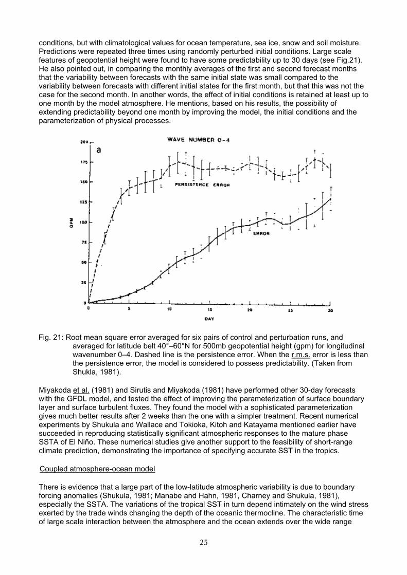
conditions, but with climatological values for ocean temperature, sea ice, snow and soil moisture. Predictions were repeated three times using randomly perturbed initial conditions. Large scale features of geopotential height were found to have some predictability up to 30 days (see Fig.21). He also pointed out, in comparing the monthly averages of the first and second forecast months that the variability between forecasts with the same initial state was small compared to the variability between forecasts with different initial states for the first month, but that this was not the case for the second month. In another words, the effect of initial conditions is retained at least up to one month by the model atmosphere. He mentions, based on his results, the possibility of extending predictability beyond one month by improving the model, the initial conditions and the parameterization of physical processes.

Fig. 21: Root mean square error averaged for six pairs of control and perturbation runs, and averaged for latitude belt 40°–60°N for 500mb geopotential height (gpm) for longitudinal wavenumber 0–4. Dashed line is the persistence error. When the r.m.s. error is less than the persistence error, the model is considered to possess predictability. (Taken from Shukla, 1981).

Miyakoda et al. (1981) and Sirutis and Miyakoda (1981) have performed other 30-day forecasts with the GFDL model, and tested the effect of improving the parameterization of surface boundary layer and surface turbulent fluxes. They found the model with a sophisticated parameterization gives much better results after 2 weeks than the one with a simpler treatment. Recent numerical experiments by Shukula and Wallace and Tokioka, Kitoh and Katayama mentioned earlier have succeeded in reproducing statistically significant atmospheric responses to the mature phase SSTA of El Niño. These numerical studies give another support to the feasibility of short-range climate prediction, demonstrating the importance of specifying accurate SST in the tropics.

Coupled atmosphere-ocean model

There is evidence that a large part of the low-latitude atmospheric variability is due to boundary forcing anomalies (Shukula, 1981; Manabe and Hahn, 1981, Charney and Shukula, 1981), especially the SSTA. The variations of the tropical SST in turn depend intimately on the wind stress exerted by the trade winds changing the depth of the oceanic thermocline. The characteristic time of large scale interaction between the atmosphere and the ocean extends over the wide range

26

from days to some thousand years. In this sense, climate model should basically be a coupled atmosphere-ocean model.

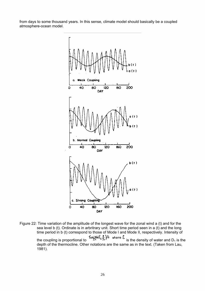
Figure 22: Time variation of the amplitude of the longest wave for the zonal wind a (t) and for the sea level b (t). Ordinate is in arbritrary unit. Short time period seen in a (t) and the long time period in b (t) correspond to those of Mode I and Mode II, respectively. Intensity of

the coupling is proportional to is the density of water and D1 is the depth of the thermocline. Other notations are the same as in the text. (Taken from Lau, 1981).

27

Theory predicts that the time-scale of the dominant process of the ocean highly depends on latitude and that it decreases with the decrease of latitude (Moore and Philander, 1977). The time required for the baroclinic Rossby waves to cross the Pacific Ocean is 9 years at 80°N, 2 years at 15°N and only 1 year near the equator after Miyakoda's (1982) estimate. In equatorial regions,

signals within the ocean propagate as Kelvin waves eastward with the speed of 2m/s, and as

Rossby waves westward with 0.5m/s (Hurlbert et al., 1976; McCreary, 1976; Philander and

Pacanowski, 1980). Because the equatorial ocean possesses such a relatively short time scale, the coupling between the atmosphere and ocean is of considerable interest and importance in the equatorial regions.

Lau (1981) constructed a very simplified coupled model in which the atmosphere is coupled with the ocean through thermal link and the ocean is coupled with the atmosphere through dynamical link. He simplified the model further to confine his study to the coupling between large-scale atmospheric and oceanic equatorial Kelvin waves only. He showed the existence of two time scales in his model. One of them (Mode I) is related to the atmospheric Kelvin wave and is mostly manifest in the atmospheric response. The other (Mode II) is related to the oceanic Kelvin wave and is the predominant mode in the equatorial climatic time-scale (see Fig.22). The time-scale and the amplitude of Mode II increases substantially with the increase of air-sea interaction. It is interesting to note that the numerical experiments of his simplified system show an El Niño-type oscillation in a baroclinic coupled system as a result of strengthening and subsequent weakening in the barotropic component of the wind.

Detailed coupled atmosphere-ocean circulation model was tried first by Manabe and Bryan (1969). They used a 1/3 sector model which is symmetric with respect to the equator and has a simplified square ocean. Later the coupled model was extended to the global model with a realistic geographical distribution of ocean without seasonal variation (Manabe et al., 1975; Bryan et al.,1979). Washington et al. (1980) also have reported a simulation study with a global realistic model with seasonal variations. All these models consider the interaction process shown in Fig. 2.

Global distribution of sea surface temperature obtained by Manabe et al. (1979) is shown in Fig. 23. This shows success in simulating basic features of seasonal variation of SST. There are, however, important differences between the simulation and the actual features. For example, the amplitude of seasonal variation of zonal mean SST in mid-latitudes of northern hemisphere is too small. The model also gives too high SST along the periphery of the Antarctic continent. The effect of Peru current and upwelling along the equator is not simulated well. Therefore, a great deal of improvement is still needed for a fully realistic simulation of the coupled atmosphere-ocean system. The resolution of the oceanic model and the treatment of the cloud amount are considered to be among the central problems.

28

Figure 23. Global distribution of SST computed with the GFDL coupled atmosphere ocean circulation model for February and August. Observed ones are also shown for comparison. (Taken from Manabe et al., 1979).

At present, it might be still too early for discussions about prediction of climatic fluctuations with the coupled atmosphere- ocean model, as no such attempts have yet been reported. However, many scientists in this field consider that the use of some kind of coupled atmosphere-ocean model is one of the most promising ways to extend the forecasting range of the climate fluctuations. We believe that comprehensive numerical models of the climate system have potentials to predict

29

essentially all the potentially predictable climate signals. Such comprehensive models adequate for seasonal forecasting, however, would require predictive capability for soil moisture, snow cover and the large-scale diabatic processes within the atmosphere as well as the SST, especially in the tropics. There are also many other problems to be considered before such a numerical model approach could be justified. Establishment of procedures for near real- time retrieval of global SST, snow cover and soil moisture will be one of the most crucial ones.

REFERENCES

Angell, J.K. and J. Korshover. 1977. Estimate of the global change in temperature, surface to 100mb between 1958 and 1975. Mon.Wea.Rev. 105:375.

Angell, J.K. and J. Korshover. 1978. Global temperature variation, surface to 100mb; an update into 1977. Mon.Wea.Rev. 106:755.

Angell, J.K. and J. Korshover. 1981. Comparison of variations in atmospheric quantities with sea-surface temperature variations in the equatorial eastern Pacific. Mon.Wea.Rev. 109:230.

Arkin, P.A. 1982. The relation between interannual variability in the 200mb tropical wind field and the Southern Oscillation. Mon.Wea.Rev. 110:1393.

Barnett, T.P. 1981. Statistical prediction of North American air temperatures from Pacific predictors. Mon.Wea.Rev. 109:1021.

Bjerknes, J. 1966. A possible response of the atmospheric Hadley circulation to equatorial anomalies of ocean temperature. Tellus. 18:820.

Bjerknes, J. 1969. Atmospheric teleconnections from the equatorial Pacific. Mon.Wea.Rev. 97:163.

Bryan, K., S. Manabe and R.C. Pacanowski. 1975. A global ocean-atmosphere climate model. Part II. The oceanic circulation, J.Phys.Oceanogr. 5:30.

Charney, J.G. and J. Shukla. 1981. Predictability of monsoon in “Monsoon Dynamics” (Sir James Lighthill and R.P. Pearce eds.) Cambridge Univ. Press.

Chervin, R.M., W.M. Washington and S.H. Schneider. 1976. Testing the statistical significance of the response of the NCAR general circulation model to North Pacific Ocean surface temperature anomalies. J.Atmos.Sci. 33:413.

Chervin, R.M., J.E. Kutzbach, D.D. Houghton and R.G. Gallimore. 1980. Response of the NCAR general circulation model to prescribed changes in ocean surface temperature. Part II. Midlatitude and subtropical changes. J.Atmos.Sci. 37:308.

Davis, R.E. 1978. Predictability of sea level pressure anomalies over the North Pacific Ocean. J.Phys.Oceanogr. 8:233.

Dickinson, R.E. 1982. Feasibility of monthly and seasonal forecasting by numerical models. “Physical basis for climate prediction on seasonal, annual and decadal time scales”. Leningrad, USSR, 13–17 September, 1982.

Fritz, S. 1982. Northern hemisphere 700mb heights and Pacific Ocean temperatures for winter Mon.Wea.Rev. 110:18.

Harnack, R.P. and H.E. Landsberg. 1978. Winter season temperature outlook by objective methods. J.Geophys.Res. 85:3601.

30

Harnack, R.P. 1979. A further assessment of winter temperature predictions using objective methods. Mon.Wea.Rev. 107:250.

Harnack, R.P. 1982. Objective winter temperature forecasts: An update and extension to the western United States. Mon.Wea.Rev. 110:287.

Horel, J.D. and T.M. Wallace. 1981. Planetary-scale atmospheric phenomena associated with the interannual variability of sea-surface temperature in the equatorial Pacific. Mon.Wea.Rev. 109:813.

Hoskins, B.J. and D.J. Karoly. 1981. The steady linear response of a spherical atmosphere to thermal and orographic forcing. J.Atmos.Sci. 38:1179.

Houghton, D.D. J.E. Kutzbach, M. McClintock and D. Suchman. 1974. Response of a general circulation model to a sea temperature perturbation, J.Atmos.Sci. 31:857.

Hurlbert, H.E., J.C. Kindel and J.J. O'Brien. 1976. A numerical simulation of the onset of El Niño. J.Phys.Oceanogr. 6:621.

Ichie, T. and J.R. Petersen. 1963. The anomalous rainfall of the 1957–58 winter in the equatorial central Pacific arid area. J.Meteor.Soc.Japan. 41:172.

Julian, P.R. and R.M. Chervin. 1978. A study of the southern Oscillation and Walker Circulation phenomena. Mon.Wea.Rev. 106:1433.

Keshavamurty, R.N. 1982. Response of the atmosphere to sea surface temperature anomalies over the equatorial Pacific and the teleconnections of the Southern Oscillation. J.Atmos.Sci. 39:124.

Kutzbach, J.E., M. Clintock and D. Suchman. 1974. Response of a general circulation model to a sea temperature perturbation. J.Atmos.Sci. 31:857.

Kutzbatch, J.E., R.M. Chervin and D.D. Houghton. 1977. Response of NCAR general circulation to prescribed changes in ocean surface temperature. Part I: Mid-latitude changes. J.Atmos.Sci. 34:1200.

Lau, Ka-M. 1981. Oscillations in a simple equatorial climate system. J.Atmos.Sci. 38:248.

McCreary, J. 1976. Eastern tropical ocean response to changing wind systems with application to El Nino. J.Phys.Oceanogr. 6:632.

Manabe, S. and K. Bryan. 1969. Climate calculations with a combined ocean-atmosphere model. J.Atmos.Sci.26:786.

Manabe, S., K. Bryan and M.J. Spelman. 1975. A global ocean-atmosphere climate model. Part I. The atmospheric circulation. J.Phys.Oceanogr. 5:3.

Manabe, S., K. Bryan and M.J. Spelman. 1979. A global ocean-atmosphere climate model with seasonal variation for future studies of climate sensitivity. Dyn.Atmos.Oceans. 3:393.

Manabe, S. and D.G. Han. 1981. Simulation of atmospheric variability. Mon.Wea.Rev. 109:2260.

Miyakoda, K. 1982. Surface boundary forcing, “Physical basis for climate prediction on seasonal, annual and decadal time scales”. Leningrad, USSR, 13–17 September 1982.

31

Miyakoda, K., T. Gordon, R. Caverly, W. Stern, J. Sirutis and W. Bourke. 1981. Simulation of a blocking event in January 1977. Preprints for Fifth conference on Numerical Weather Prediction, 2–6 November 1981. Monterey, CA, 99.

Moore, D.W. and S.G.H. Philander. 1977. Modeling of the tropical oceanic circulation. In The Sea, 6, Interscience, New York.

Moura, D.A. and J. Shukla. 1981. On the dynamics of droughts in northeast Brazil: observations, theory and numerical examples with a general circulation model. J.Atmos.Sci. 38:2653.

Namias, J. 1968. Long-range weather forecasting history, current status and outlook. Bull.Amer.Meteor.Soc. 49:438.

Namias, J. 1969. Seasonal interactions between the Northern Pacific Ocean and the atmosphere during the 1960's. Mon.Wea.Rev. 97:173.

Namias, J. 1971. The 1968–69 winter as an outgrowth of sea and air coupling during antecedent seasons. J.Phys.Oceanogr. 1:65.

Namias, J. 1972. Experiments in objectively predicting some atmospheric and oceanic variables for the winter of 1971–72. J.Appl.Meteor. 11:1164.

Namias, J. 1976. Negative ocean-air feedback systems over the North Pacific in the transition from warm to cold season. Mon. Wea. Rev. 104:1107.

Namias, J. 1982. Case studies of long period air-sea interactions relating to long range forecasting. “Physical basis for climate prediction on seasonal, annual and decadal time scales”. Leningrad, USSR. 13–17 September, 1982.

Namias, J. and R.M. Born. 1970. Temporal coherence in North Pacific Ocean and the atmosphere during the 1960's. Mon. Wea. Rev. 97:173.

Namias, J. and D.R. Cayan. 1981. Large-scale air-sea interactons and short-period climatic fluctuations. Science. 214:869.

Nap, J.L., H.M. Van den Dool and J. Oerlemans. 1981. A verification of monthly weather forecasts in the seventies. Mon. Wea. Rev. 109:306.

Newell, R.E. and B.C. Weare. 1976. Ocean temperatures and large scale atmospheric variations. Nature. 262–40.

Nicholls, N. 1980. Long-range weather forecasting: Value, status and prospects. Rev. Geophys. Space Phys. 18:771.

Oort, A.H. and T.H. Vonder Haar. 1976. On the observed annual cycle in the Ocean-atmosphere heat balance over the northern hemisphere. J.Phys.Oceanogr. 6:781.

Philander, S.G.H. and R.C. Pacanowski. 1980. The generation of equatorial of equatorial currents. J. Geophys. Res. 85:1123.

Rasmusson, E.G. and T.H. Carpenter. 1982. Variation in tropical sea surface temperature and surface wind fields associated with the Southern Oscillation/El Nino. Mon. Wea. Rev. 110:254.

32

Rogers, J.C. and H. van Loon. 1979. The seesaw in winter temperatures between Greenland and Northern Europe. Part II: Some oceanic and atmospheric effects in middle and high latitudes. Mon. Wea. Rev. 107:509.

Rogers, J.C. and H. van Loon. 1982. Spatial variability of sea level pressure and 500mb height anomalies over the southern hemisphere. Mon. Wea. Rev. 110:1375.

Rowntree, P.R. 1972. The influence of tropical East Pacific Ocean temperature on the atmosphere. Quart. J. Roy. Meteor. Soc. 98:290.

Rowntree, P.R. 1976. Tropical forcing of atmospheric motions in a numerical model. Quart. J. Roy. Meteor. Soc. 102:583.

Shukla, J. 1975. Effects of Arabian Sea-surface temperature in Indian summer monsoon: A numerical experiment with GFDL mode. J.Atmos. Sci. 32:503.

Shukla, J. 1981. Dynamic predictability of monthly means. J.Atmos. Sci. 38:2547.

Shukla, J. and B.M. Misra. 1977. Relationships between sea surface temperature and wind speed over the central Arabian Sea and monsoon rainfall over India. Mon.Wea.Rev. 105:998.

Sirutis, J. and K. Miyakoda. 1981. Comparative integrations of global models with various parameterized processes of sub-grid scale vertical eddy transports. Preprints for Fifth conference on Numerical Weather Prediction. 2–6 November 1981. Monterey, CA 106.

Trenberth, 1976. Spatial and temporal variations of the Southern Oscillation. Quart.J.Roy.Meteor.Soc. 102:639.

van Loon. H. and R.A. Madden. 1981. The Southern Oscillation. Part I. Global associations with pressure and temperature in northern winter. Mon.Wea.Rev. 109:1150.

van Loon, H. and J.C. Rogers. 1981. The Southern Oscillation. Part II. Association with canges in the middle troposphere in the northern winter. Mon.Wea.Rev. 109:1163.

Wallace, J.M. and D.S. Gutzler. 1981. Teleconnections in the geopotential height field during the northern hemisphere winter. Mon.Wea.Rev. 109:784.

Walsh, J.E. and M.B. Richman. 1981. Seasonality in the associations between surface temperatures over the United States and the North Pacific Ocean. Mon.Wea.Rev. 109:767.

Washington, W.M., A.J.Semtner, Jr., G.A. Meehl, D.J. Knight and T.A. Mayer. 1980. A general circulation experiment with a coupled atmosphere, ocean and sea ice model. J.Phys.Oceanogr. 10:1887.

Weare, B.C. 1977. Empirical orthogonal analaysis of Atlantic Ocean surface temperature. Quart.J.Roy.Meteor.Soc. 103:467.

Weare, B.C. 1979. A statistical study of the relationships between ocean surface temperatures and the Indian monsoon. J.Atmos.Sci. 36:2279.

Weare, B.C., A.R. Navato, and R.E. Newell. 1976. Empirical orthogonal analysis of Pacific sea surface temperatures. J.Phys.Oceanogr. 6:671.

Webster, P.J. 1981. Mechanisms determining the atmospheric response to sea surface temperature anomalies. J.Atmos.Sci. 38:554.

33

Webster, P.J. 1982. Seasonality in the local and remote atmospheric response to sea surface temperature anomalies. J.Atmos.Sci. 39:41.

Wright, P.B. 1979. A simple model for simulating regional short-term climatic changes. Mon.Wea.Rev. 107:1567.

Wyrtki, K. 1975. El Niño - the dynamic response of the equatorial Pacific Ocean to atmospheric forcing. J.Phys.Oceanogr. 5:572.

Yamamoto, R., T. lwashima and M. Hoshiai. 1975. Change of the surface air temperature averaged over the northern hemisphere and large volcanic eruptions during the year 1951–1972. J. Meteor.Soc.Japan. 53:482.

Yamamoto, R. and M. Hoshiai. 1979. Recent change of the northern hemisphere mean surface air temperature estimated by optimum interpolation. Mon.Wea.Rev. 107:1239.