part ii general relativity - university of cambridge · part ii general relativity lecture notes...
TRANSCRIPT

Part II General Relativity
Lecture Notes
Abstract
These notes represent the material covered in the Part II lecture General Relativity(GR). While the course is largely self-contained and some aspects of Newtonian Gravityand Special Relativity will be reviewed, it is assumed that readers will already be famil-iar with these topics. Also, calculus in N dimensions and Linear Algebra will be usedextensively without being introduced.
This set of notes differs from the long version by representing in almost verbatim stylehow the material is presented in the lecture room. It is primarily designed to dispensewith the necessity to take notes during the lectures.
A more in-depth discussion of books is given in the long set of notes. Here we merelydiscuss a few books seemingly most suitable for an introduction to general relativity.
• S. M. Carroll: “Spacetime and Geometry: An Introduction to General Relativity”[2] ; cf. also [1] .
• R. d’Inverno: “Introducing Einstein’s Relativity” [3] .
• J. B. Hartle: “Gravity, An Introduction to Einstein’s General Relativity” [4] .
• L. Ryder: “Introduction to General Relativity” [5] .
• B. Schutz, “A first course in general relativity” [6] .
I would not set any of them apart over the others, but recommend each reader to have alook at them and find where the best chemistry is found.
Example sheets will be pointed to at some later stage, probably on
http://www.damtp.cam.ac.uk/user/examples
Lectures Webpage:
http://www.damtp.cam.ac.uk/user/us248/Lectures/lectures.html
Cambridge, Dec 10 2016
Ulrich Sperhake
1

CONTENTS 2
Contents
A Preliminaries 4A.1 Units . . . . . . . . . . . . . . . . . . . . . . . . . . . . . . . . . . . . . . . . . . 4A.2 Newtonian Gravity . . . . . . . . . . . . . . . . . . . . . . . . . . . . . . . . . . 6A.3 Special Relativity . . . . . . . . . . . . . . . . . . . . . . . . . . . . . . . . . . . 11
B Differential geometry 16B.1 Manifolds and tensors . . . . . . . . . . . . . . . . . . . . . . . . . . . . . . . . 16B.2 The metric tensor . . . . . . . . . . . . . . . . . . . . . . . . . . . . . . . . . . . 22B.3 Geodesics . . . . . . . . . . . . . . . . . . . . . . . . . . . . . . . . . . . . . . . 24B.4 Covariant derivative . . . . . . . . . . . . . . . . . . . . . . . . . . . . . . . . . 27B.5 The Levi-Civita connection . . . . . . . . . . . . . . . . . . . . . . . . . . . . . . 29B.6 Parallel transport . . . . . . . . . . . . . . . . . . . . . . . . . . . . . . . . . . . 30B.7 Normal coordinates . . . . . . . . . . . . . . . . . . . . . . . . . . . . . . . . . . 31B.8 The Riemann tensor . . . . . . . . . . . . . . . . . . . . . . . . . . . . . . . . . 33
C Physical laws in curved spacetimes 38C.1 The covariance principle . . . . . . . . . . . . . . . . . . . . . . . . . . . . . . . 38C.2 The energy momentum tensor . . . . . . . . . . . . . . . . . . . . . . . . . . . . 38C.3 The Einstein equations . . . . . . . . . . . . . . . . . . . . . . . . . . . . . . . . 41
D The Schwarzschild solution and classic tests of GR 42D.1 Schwarzschild’s solution . . . . . . . . . . . . . . . . . . . . . . . . . . . . . . . 42D.2 Geodesics in the Schwarzschild spacetime . . . . . . . . . . . . . . . . . . . . . . 43D.3 Classic tests of GR . . . . . . . . . . . . . . . . . . . . . . . . . . . . . . . . . . 47D.4 The causal structure of the Schwarzschild spacetime . . . . . . . . . . . . . . . . 51D.5 Hawking radiation . . . . . . . . . . . . . . . . . . . . . . . . . . . . . . . . . . 58
E Cosmology 59E.1 Homogeneity and isotropy . . . . . . . . . . . . . . . . . . . . . . . . . . . . . . 59E.2 The Friedmann equations . . . . . . . . . . . . . . . . . . . . . . . . . . . . . . 61E.3 Cosmological redshift . . . . . . . . . . . . . . . . . . . . . . . . . . . . . . . . . 62E.4 Cosmological models . . . . . . . . . . . . . . . . . . . . . . . . . . . . . . . . . 64
F Singularities and geodesic incompleteness 70F.1 Coordinate vs. physical singularities . . . . . . . . . . . . . . . . . . . . . . . . 70F.2 Geodesic incompleteness . . . . . . . . . . . . . . . . . . . . . . . . . . . . . . . 70
G Linearized theory and gravitational waves 72G.1 Plane waves and pp metrics . . . . . . . . . . . . . . . . . . . . . . . . . . . . . 72G.2 Linearized theory . . . . . . . . . . . . . . . . . . . . . . . . . . . . . . . . . . . 72G.3 The Newtonian limit . . . . . . . . . . . . . . . . . . . . . . . . . . . . . . . . . 74G.4 Gravitational waves . . . . . . . . . . . . . . . . . . . . . . . . . . . . . . . . . . 75

CONTENTS 3
G.5 The quadrupole formula . . . . . . . . . . . . . . . . . . . . . . . . . . . . . . . 76

A PRELIMINARIES 4
A Preliminaries
A.1 Units
SI units: • metres, second, kilogram etc.
• Adapted to “ourselves” → numbers O(1)
Natural units: • Take into account constants of nature.
→ 1) unifies physical dimensions (space, time etc.)
2) indicate possible breakdown of theories
• Better adapted to extreme physics.
Speed of light
c = 299 792 458 m/s ≈ 3× 10⁸ m/s!
= const
Suggests to measure all speeds in units of c.
⇒ c = 3.00× 10⁸ m/s!
= 1
⇒ 1 s = 3.00× 10⁸ m
Familiar from the light year: 1 yr = 9.4607× 10¹⁵ m
v c = 1 ⇒ Galileo trafo, Newtonian kinematics accurate
v . 1 ⇒ both break down → need special relativity (SR)
Gravitational constant
G = 6.67408× 10⁻¹¹ m3
kg s2
!= const
Set c = 1, G = 1 ⇒ 1 m = 1.3466× 1027 kg or 1 s = 4.0370× 1035 kg
Example: Solar mass M = 1.4771 km = 4.9269 µs → ∼ Schwarzschild radius of sun
M
R c2
G= 1 ⇒ Newtonian gravity (NG) accurate
M
R≈ 1 ⇒ NG breaks down → need general relativity (GR)

A PRELIMINARIES 5
Comment: If velocities determined by gravity, the regimes v ≈ 1 and M/R ≈ 1 overlap.
E.g.: (1) Spherical orbit around mass M :v2
c2=G
c2
M
R⇒ v2 =
M
R
(2) Escape velocity from sphere of mass M :v2e
c2=
2G
c2
M
R⇒ v2
e =2M
R
Planck’s constant
~ ..=h
2π= 1.0545718× 10⁻³⁴ kg m2
s
Set c = 1, ~ = 1 ⇒ 1 kg = 8.5223× 1050 Hz or 1 m =1
3.51767288× 10−43 kg
Compton wavelength: λ =~mc
=1
m
Compare Compton wavelength of a body with its size or available volume.
E.g. : Sun: λ =~
Mc= 0.177× 10−72 m ⇒ λ
R 1
Proton: λp =~mpc
= 0.210268 fm ∼ radius of atomic nuclei ∼ 1 . . . 10 fm
λ
R 1 ⇒ Classical physics accurate
λ
R≈ 1 ⇒ Need quantum mechanics (QM)
Planck mass
Consider a system withG
c2
M
R= 1 (GR!) and
~McR
= 1 (QM!).
⇒ M =
√~cG
= 2.18× 10⁻⁸ kg = 1.22× 10¹⁹ GeV
In this regime, quantum and GR effects are important.
The theory of quantum gravity for this regime remains unknown.
A PRELIMINARIES 6
A.2 Newtonian Gravity
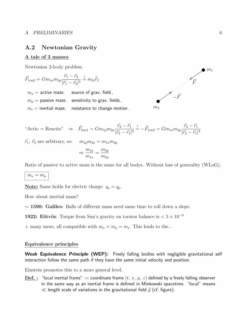
A tale of 3 masses
Newtonian 2-body problem
~F1on2 = Gm1am2p~r1 − ~r2
|~r1 − ~r2|3!
= m2i~r2
ma = active mass: source of grav. field ,
mp = passive mass: sensitivity to grav. fields ,
mi = inertial mass: resistance to change motion .
−~F
m2
m1
~F
“Actio = Reactio” ⇒ ~F2on1 = Gm1pm2a~r2 − ~r1
|~r2 − ~r1|3!
= −~F1on2 = Gm1am2p~r2 − ~r1
|~r2 − ~r1|3
~r1, ~r2 are arbitrary, so: m1pm2a = m1am2p
⇒ m1p
m1a
=m2p
m2a
Ratio of passive to active mass is the same for all bodys. Without loss of generality (WLoG),
ma = mp
Note: Same holds for electric charge: qa = qp.
How about inertial mass?
∼ 1590: Galileo: Balls of different mass need same time to roll down a slope.
1922: Eotvos: Torque from Sun’s gravity on torsion balance is < 5× 10⁻⁹
+ many more, all compatible with ma = mp = mi. This leads to the...
Equivalence principles
Weak Equivalence Principle (WEP): Freely falling bodies with negligible gravitational selfinteraction follow the same path if they have the same initial velocity and position.
Einstein promotes this to a more general level.
Def. : “local inertial frame” ..= coordinate frame (t, x, y, z) defined by a freely falling observerin the same way as an inertial frame is defined in Minkowski spacetime. “local” means length scale of variations in the gravitational field ~g (cf. figure).
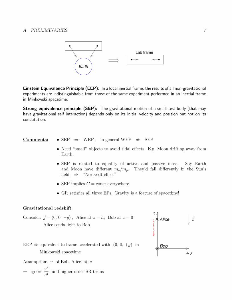
A PRELIMINARIES 7
Earth
Lab frame
Einstein Equivalence Principle (EEP): In a local inertial frame, the results of all non-gravitationalexperiments are indistinguishable from those of the same experiment performed in an inertial framein Minkowski spacetime.
Strong equivalence principle (SEP): The gravitational motion of a small test body (that mayhave gravitational self interaction) depends only on its initial velocity and position but not on itsconstitution.
Comments: • SEP ⇒ WEP ; in general WEP ; SEP
• Need “small” objects to avoid tidal effects. E.g. Moon drifting away fromEarth.
• SEP is related to equality of active and passive mass. Say Earthand Moon have different ma/mp. They’d fall differently in the Sun’sfield ⇒ “Nortvedt effect”
• SEP implies G = const everywhere.
• GR satisfies all three EPs. Gravity is a feature of spacetime!
Gravitational redshift
Consider: ~g = (0, 0, −g) , Alice at z = h, Bob at z = 0
Alice sends light to Bob.
Bob
x, y
g
z
Alice
EEP ⇒ equivalent to frame accelerated with (0, 0, +g) in
Minkowski spacetime
Assumption: v of Bob, Alice c
⇒ ignorev2
c2and higher-order SR terms

A PRELIMINARIES 8
⇒ zA(t) = h+1
2gt2 , zB(t) =
1
2gt2 , vA = vB = gt
! c .
• Alice emits first signal at t1
⇒ z1(t) = zA(t1)− c(t− t1) = h+1
2gt21 − c(t− t1)
• This reaches Bob at T1, i.e. h+1
2gt21 − c(T1 − t1) =
1
2gT 2
1 (∗∗)
• Alice emits second signal at t2 = t1 + ∆τA .
This reaches Bob at T2 = T1 + ∆τB .
⇒ h+1
2g(t1 + ∆τA)2 − c(T1 + ∆τB − t1 −∆τA) =
1
2g(T1 + ∆τB)2
∣∣∣∣ subtract (∗∗)
⇒ c(∆τA −∆τB) +1
2g∆τA (2t1 + ∆τA) =
1
2g∆τB (2T1 + ∆τB)
• Assumption: ∆τA t1 , ∆τB T1 , e.g. period in light waves
⇒ c(∆τA −∆τB) + g∆τA t1 = g∆τB T1
⇒ ∆τB (gT1 + c) = ∆τA (gt1 + c)
⇒ ∆τB =
(1 +
gT1
c
)−1(1 +
gt1c
)∆τA ≈
[1− g(T1 − t1)
c
]∆τA
∣∣∣∣ we usedgt
c 1
• (∗∗) ⇒ h
c− (T1 − t1) =
1
2
g
c(T1 + t1)︸ ︷︷ ︸ 1
(T1 − t1) ≈ 0
∣∣∣∣ we usedgt
c 1
⇒ T1 − t1 =h
cto leading order.
• ⇒ ∆τB ≈(
1− gh
c2
)∆τA
!< ∆τA
⇒ Signal appears blue shifted to Bob: c∆τB = λB ≈(
1− gh
c2
)λA
Confirmed in Pound-Rebka experiment (1960): light falling in tower.
Light climbing out of a gravity well is red shifted.
Redshift in curved spacetime
Recall: Invariant interval in SR: c2∆τ 2 = c2 ∆t2 −∆x2 −∆y2 −∆z2
For weak, static gravitational field, this generalizes to (cf. later):
A PRELIMINARIES 9
c2 dτ 2 =
[1 +
2φ(x, y, z)
c2
]c2dt2 −
[1− 2φ(x, y, z)
c2
](dx2 + dy2 + dz2) ;
φ
c2 1
• Alice: ~xA , Bob: ~xB , at fixed positions!
• Alice emits signals at tA, tA + ∆t
Bob receives the first at tB . When does he see the second?
• The spacetime is static: φ does not depend on t
⇒ The two signals travel on identical trajectories, just shifted in time
⇒ Bob receives the second signal at tB + ∆t .
• But what proper times do Alice’s and Bob’s clocks measure?
∆τ 2A =
(1 +
2φAc2
)∆t2 ,
⇒ ∆τA ≈(
1 +φAc2
)∆t ,
∆τ 2B =
(1 +
2φBc2
)∆t2
⇒ ∆τB ≈(
1 +φBc2
)∆t ,
⇒ ∆τB ≈(
1 +φBc2
) (1 +
φAc2
)−1
∆τA ≈(
1 +φB − φA
c2
)∆τA
Newtonian gravity for matter fields
Index notation:
• Write vectors, matrices as components: xi = (x1, x2, x3) = (x, y, z); vi = (v1, v2, v3) etc.
• Repeated indices in a product are summed over: Aijvj ..=3∑j=1
Aijvj
• No index may appear more than twice: Aiivi is not defined.
• We may rename indices summed over: Aijvj = Aikvk
• In an equation or a sum, free (not repeated) indices must match on both sides:
wi + Aikvk = 0 is correct; wj = Aikvk is not.
• We denote partial derivatives by ∂i =∂
∂xi. Sometimes, we also use a comma:
vk,i ..= ∂ivk =∂vk∂xi

A PRELIMINARIES 10
Example: Motion of point particle in gravitational field ~g.
m~x = m~g(~x, t) ⇒ xi = gi(xk, t).
Let xi be a non-inertial coordinate system: xi = xi − bi(t).
⇒ ¨xi = g(xk, t) = gi(xk, t)− bi(t)
Comments: 1) If gi is uniform (xk independent) ⇒ ∃ bi such that gi = 0.
2) gi not uniform ⇒ we can only get gi = 0 locally → freely falling frame
Index version of Newtonian gravity
Tidal forces on two particles at xi, xi + δxi :
d2
dt2xi = gi(xj, t) ,
d2
dt2(xi + δxi) = gi(xj + δxj, t)
⇒ d2
dt2δxi = δxk∂kgi +O(δx2
j) ,
⇒ d2
∂t2δxi + Eijδxj = 0 , Eij ..= −∂jgi .
~g is curl free ⇒ ~g = −~∇φ ⇔ gi = −∂iφ
It follows: Eij = Eji .
Poisson equation: ~∇ · ~g = −4πGρ ⇒ ~∇2φ = ∂i∂iφ = 4πGρ ⇒ Eii = 4πGρ .
The definition Eij = −∂jgi implies
∂kEij = −∂k∂jgi = ∂jEki ⇒ Ei[j,k]..=
1
2(Eij,k − Eik,j) = 0
The need for GR: not so much from experiment, but the incompatibility of SR with Newto-nian space and time.

A PRELIMINARIES 11
A.3 Special Relativity
Extend index notation
• Distinguish upstairs and downstairs indices: vi 6= vi.
• Summation only over one up and one downstairs index: vjuj ..=3∑j=1
vjuj .
• Latin indices i, j, . . . = 1, 2, 3. Greek indices α, β, . . . = 0 . . . 3.
Metric
Pythagoras as matrix equation: ∆s2 = ∆x2 + ∆y2 + ∆z2 = δij∆xi ∆xj (†)
δij = diag(1, 1, 1) = flat Euclidean metric in Cartesian coords.
In polar coordinates: ds2 = dx2 + dy2 + dz2
= dr2 + r2dθ2 + r2 sin2 θ dφ2
= gijdxidxj , gij = diag(1, r2, r2 sin2 θ) .
Note: Unlike (†), this only works for infinitesimal distances!
Lorentz transformations
Consider inertial (non-accelerated) frames with Cartesian coords.
Proper distance between spacetime events (t, x, y, z) and (t+ ∆t, x+ ∆x, y + ∆y, z + ∆z):
∆s2 = −∆t2 + ∆x2 + ∆y2 + ∆z2
In SR, no inertial frame is prefered over another ⇒ same proper distance in xα:
∆s2 = −∆t2 + ∆x2 + ∆y2 + ∆z2
Note: For ∆s = 0, the events are connected by a light ray.
⇒ All inertial frames measure the same speed of light.
Index notation: ∆s2 = ηαβ∆xα∆xβ = ηαβ∆xα∆xβ
ηαβ = ηαβ =
−1 0 0 00 1 0 00 0 1 00 0 0 1
⇔ ηαβ = ηαβ =
−1 0 0 00 1 0 00 0 1 00 0 0 1
ηαβ is the inverse of ηαβ.

A PRELIMINARIES 12
Inertial frames are related by xα = Λαµx
µ + xµ0 , Λαµ = const
WLoG: xµ0 = 0.
z
y
x
~v
z
y
x
We want: ηαβ∆xα∆xβ = ηαβΛαµ∆xµ Λβ
ν∆xν !
= ηµν∆xµ ∆xν
⇒ ηµν = ΛαµΛβ
νηαβ
One can show that this is satisfied by the Lorentz transformations
Λαµ =
γ −γv 0 0−γv γ 0 0
0 0 1 00 0 0 1
⇔ Λµα =
γ γv 0 0γv γ 0 00 0 1 00 0 0 1
, γ =1√
1− v2
Comments • WLoG, coordinates oriented such that the velocity v points in the x direction
• One can show ΛαµΛµ
β = δαβ , ΛµαΛα
ν = δµν
World lines and 4-velocity
Def.: The interval between two spacetime events xα and xα + ∆xα is called
timelike :⇔ ηµν∆xµ ∆xν < 0
null :⇔ ηµν∆xµ ∆xν = 0
spacelike :⇔ ηµν∆xµ ∆xν > 0 .
Def.: Proper time ∆τ 2 ..= −∆s2 = ∆t2 −∆x2 −∆y2 −∆z2

A PRELIMINARIES 13
Postulate: A clock moving on a world line xα(λ) , λ ∈ R, that is in every point timelike or null,measures the proper time along this world line
τ ..=
∫ λ2
λ1
√−ηµν
dxµ
dλ
dxµ
dλdλ . (‡)
Comments: • τ is invariant under reparametrizing λ→ µ(λ).
• We often parametrize timelike curves with τ
• (‡) ⇒ dτ =
√−ηµν
dxµ
dτ
dxν
dτdτ ⇒ ηµν x
µxν ..= ηµνdxµ
dτ
dxν
dτ= −1
Def.: The four velocity along a timelike curve is uα ..=dxα
dτ
By def. ηµνuµuν = −1
Geodesics
Consider the action S[xα(λ)] =
∫ √−ηαβ
dxα
dλ
dxβ
dλ︸ ︷︷ ︸=..L
dλ
Geodesics are curves that extremize this action.
They follow from the Euler-Lagrange (EL) equations
d
dλ
∂L∂xµ
=∂L∂xµ
⇒ . . . ⇒ d2xα
dτ 2= 0 .
One can derive the same equation for null and spacelike geodesics (cf. GR case below).
Postulate: Free massive (massless) particles in special relativity move on straight timelike (null)curves,
d2xα
dτ 2= 0 . (A.1)
A PRELIMINARIES 14
Time dilation
Let O, O be 2 observers with coordinates xµ, xα.
Let O move with v in the x direction relative to O.
Clock at rest in O: uα =
(dt
dτ, 0, 0, 0
)
Viewed from O: uµ =
(dt
dτ,dxi
dτ
)!
= Λµαu
α =
(γdt
dτ, γv
dt
dτ, 0, 0
)(†)
ut component:dt
dτ= γ
dt
dτ⇒ dt
dt= γ
⇒ dt =dt√
1− v2: O sees the moving O age more slowly.
Lorentz contraction
Def.: Length of a rod in O ..= proper distance ∆s between two events A and B, where xiA is theposition of the rod’s tail at a specified time tA = t0 and xiB is the position of the rod’s headat the same time tB = t0.
∆s =√ηαβ∆xα∆xβ =
√δij∆xi∆xj , ∆xi = xiB − xiA (A.2)
Let the rod be at rest in O.
World lines of head and tail: xµ = (ttail, xi0) , yµ = (thead, x
i0 + ∆xi)
O will pick events with ttail = thead ⇒ `2 = ∆s2 = δij∆xi∆xj
World lines in O: (ttail, xi) = xα = Λα
µxµ
(thead, yi) = yα = Λα
µyµ = Λα
µ(xµ + ∆xµ)
O will pick events A, B with ttail = thead.
⇒ . . .⇒ ttail = thead +Λ0
i ∆xi
Λ00
= thead − vi∆xi
Proper distance ∆s2AB
: xµA = (thead − vi∆xi, xi0) , xµB = (thead, xi0 + ∆xi)
⇒ ˜2 = ∆s2AB = ηµν(x
µ
B − xµ
A)(xνB − xνA)
= −(vi∆xi)2 + δij∆x
i ∆xj

A PRELIMINARIES 15
Orient the rod along the x axis ⇒ ` = ∆x , ˜=√
1− v2x∆x
Comments: • The sign of v does not matter.
• Velocity perpendicular to the rod causes no contraction.
Four momentum and Doppler shift
Def.: Four momentum of a particle with rest mass m and 4-velocity uµ: pα = muα
ηµνuµuν = −1 ⇒ ηµνp
µpν = −m2
Let O move with v in x direction relative to O; consider particle at rest in O.
⇒ pα = (m, 0, 0, 0)
pµ = Λµαp
α = γm(1, v, 0, 0)
γm = total relativistic energy of particle in O
γmv = linear momentum of particle in O
⇒ pµ = (E, p, 0, 0)
ηµνpµpν = −E2 + p2 = −m2 ⇒ E2 = m2c4 + p2c2
Comment: Null curves do not have a four velocity (unit tangent vector), but they have afour momentum.
Recall for massless particles: E = hν, p = h/λ.
⇒ pα = hν(1, 1, 0, 0) e.g. photon moving in x direction
Now consider such a photon and let O move with v in x-direction relative to O.
⇒ in O: pα = (E, E, 0, 0) , E = hν
⇒ in O: pα = Λαµp
µ =(γE − γvE, − γvE + γE, 0, 0
)=..(E, E, 0, 0
), E = hν
Redshiftν
ν=E
E= γ(1− v) =
√1− v1 + v
Note: • Redshift if O moves in same direction as photon. Blueshift if v < 0.
• Transverse Doppler shift if v perpendicular to propagation of photon.
More complicated to calculate!

B DIFFERENTIAL GEOMETRY 16
B Differential geometry
Goal: Extend Euclidean geometry to curved spaces.
Motivation: GR generalizes SR like Riemannian geometry generalizes Euclidean geometry.
Conventions: • An upstairs index in a denominator counts as a downstairs index.
E.g.: ∂i ..=∂
∂xi
• Contravariant indices: upstairs. Covariant indices: downstairs.
B.1 Manifolds and tensors
Strategy: Start with manifold M. Establish structure on M step by step.
Def.: n dimensional manifoldM ..= set of points that locally resembles Euclidean space Rn ateach point. For our purposes, this means that there exists a one-to-one and onto map
φ :M→ U ⊂ Rn , p ∈M 7→ xα ∈ U ⊂ Rn , α = 0, . . . , n− 1 , (B.1)
where U is an open subset of Rn. xα are the coordinates on M.
M
p
xα
U ⊂ R
φ
B DIFFERENTIAL GEOMETRY 17
Comments: • It is sufficient if we can chop up M and map each piece separately to Rn.Everything we will develop also holds for such subdivisions of M.
• Think of coordinates like house numbers in a street. Houses don’t change ifwe change their numbers. Likewise, we will find objects onM to be invariantunder coordinate changes.
• Curves, vectors etc. live on M, not in the coordinate space. But φ is one-to-one, so this distinction often blurred.
Functions and curves
Def.: Function on M: f :M→ R
f is smooth :⇔ ∀ coordinate systems xα: f(xα) is a smooth function from Rn to R. If fis invariant under a change of coordinates, it is a scalar.
Def.: Curve ..= a map λ : I ⊂ R→M, I open. λ is smooth :⇔ ∀ coordinate systems xα: themap xα λ : I → Rn is smooth
Vectors
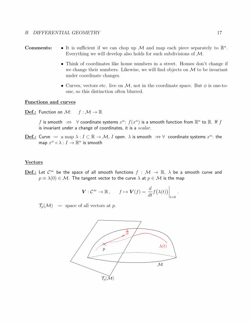
Def.: Let C∞ be the space of all smooth functions f : M → R, λ be a smooth curve andp ≡ λ(0) ∈M. The tangent vector to the curve λ at p ∈M is the map
V : C∞ → R , f 7→ V (f) =d
dtf(λ(t)
)∣∣∣∣t=0
.
Tp(M) ..= space of all vectors at p.
λ(t)
M
p
ddt
Tp(M)
B DIFFERENTIAL GEOMETRY 18
A vector is a derivative operator! It obeys:
(i) Linearity: α, β ∈ R, f, g ∈ C∞ ⇒ V (αf + βg) = αV (f) + βV (g)
(ii) Leibniz rule: f, g ∈ C∞ ⇒ V (f g) = V (f) g(p) + f(p)V (g)
Consider coordinates xα ⇒ V (f) =d
dtf(xµ(λ(t)
))=dxµ
dt
∣∣∣∣λ
∂
∂xµf(xα)
↑
vector components basis vectors
One can show: Tp(M) has dimension n and eµ ..= ∂µ ..=∂
∂xµform a basis.
Components: V µ =dxµ
dt⇒ V = V µeµ = V µ∂µ =
dxµ
dt
∂
∂xµ=
d
dt
Coordinate change xµ → xα: eµ =∂
∂xµ→ eα =
∂
∂xα=∂xµ
∂xα∂
∂xµ=∂xµ
∂xαeµ
V µ =dxµ
dt→ V α =
dxα
dt=∂xα
∂xνdxν
dt=∂xα
∂xνV ν
⇒ V = V µeµ = V αeα is invariant!
∂µ is a coordinate basis. Non-coordinate bases also exist but we do not consider them.
Covectors / one-forms
Def.: A covector or one-form is a linear map
η : Tp(M)→ R , V 7→ η(V )
T ∗p (M) ..= Cotangent space of all covectors at p ∈M. T ∗p (M) is an n dimensional vectorspace. Let eµ be a basis of Tp(M). The components of a covector η are ηµ ..= η(eµ).
Properties: Linearity: α, β ∈ R, V , W ∈ Tp(M) ⇒ η(αV + βW ) = αη(V ) + βη(W )
Components: η(V ) = η(V µeµ) = V µη(eµ) = V µηµ
Transformation rule: We require η(V ) to be a scalar
⇒ η(V ) = ηµVµ !
= ηαVα = ηα
∂xα
∂xµV µ ⇒ ηβ =
∂xµ
∂xβηµ

B DIFFERENTIAL GEOMETRY 19
Def.: Gradient df of a smooth function f : df : Tp(M)→ R ,d
dt7→ df
dt
Let V =d
dt∈ Tp(M) ⇒ df(V ) =
df
dt= V (f)
Basis: Let f = xα , α fixed ⇒ dxα(eβ) = dxα(
∂
∂xβ
)=∂xα
∂xβ= δαβ
⇒ ηαdxα(V ) = ηαdx
α(V β∂β) = ηαVβdxα(∂β) = ηαV
βδαβ = ηαVα = η(V )
⇒ η = ηαdxα
Tensors
Def. : A tensor T at p ∈M of rank(rs
), r, s ∈ N0, is a multilinear map
T : T ∗p (M)× . . .× T ∗p (M)︸ ︷︷ ︸r factors
×Tp(M)× . . .× Tp(M)︸ ︷︷ ︸s factors
→ R
Plug in r one-forms and s vectors and out pops a real number.
Examples: • Covector η = tensor of rank(
01
): input V , output η(V )
• Vector V can be viewed as: V : T ∗p (M)→ R , η 7→ η(V )
⇒ V is a(
10
)tensor.
Components of V : η(V ) = ηαdxα(V ) = ηαV
α ⇒ V α = dxα(V ) = V (dxα)
This holds for all tensors: Tα1...αrβ1...βs = T (dxα1 , . . . , dxαr , eβ1 , . . . , eβs)
• δ : T ∗p (M)× Tp(M)→ R , (η,V ) 7→ η(V ) ∀ η ∈ T ∗p (M) , V ∈ Tp(M)
is a(
11
)tensor with components δ(dxα, ∂β) = dxα(∂β) =
∂xα
∂xβ= δαβ
One can show that tensors of rank(rs
)form a vector space of dimension nr+s and transform
according to
Tα1...αrβ1...βs =
∂xα1
∂xµ1. . .
∂xαr
∂xµr∂xν1
∂xβ1. . .
∂xνs
∂xβsT µ1...µrν1...νs

B DIFFERENTIAL GEOMETRY 20
Tensor operations
(1) Addition, scalar multiplication: Let c1, c2 ∈ R, S, T(
11
)tensors
⇒ c1S + c2T : T ∗p (M)× Tp(M)→ R , η, V 7→ c1S(η,V ) + c2T (η,V )
(2) (Anti-) symmetrization: E.g. for(
02
)tensor T
symmetric part: Sαβ ..=1
2(Tαβ + Tβα) =.. T(αβ)
antisymm. part:1
2(Tαβ − Tβα) =.. T[αβ]
Index subset: T (αβ)γδ
..=1
2(Tαβγδ + T βαγδ)
non-adjacent indices: T(α|βγ|δ)..=
1
2(Tαβγδ − Tδβγα)
Over n > 2 indices: • sum over all permutations
• apply sign of permutation for anti-symm.
• divide by n!
E.g.: Tα[βγδ] =1
3!
(Tαβγδ + Tαδβγ + Tαγδβ − Tαδγβ − Tαγβδ − Tαβδγ
)
(3) Contraction of(rs
)tensor ..= Summation over 1 upper and 1 lower index
→(r−1s−1
)tensor
Example: Let T be a(
32
)tensor
⇒(
21
)tensor S(ω,η,V ) ..= T (dxµ,ω,η, ∂µ,V )
This is basis independent:
T(dxµ,ω,η,
∂
∂xµ,V)
=∂xµ
∂xα∂xβ
∂xµ︸ ︷︷ ︸=δβα
T(dxα,ω,η,
∂
∂xβ,V)
= T (dxα,ω,η, ∂α,V )
Components: Sµνρ = Tαµναρ

B DIFFERENTIAL GEOMETRY 21
(4) Let S be a(pq
)tensor, T a
(rs
)tensor
“outer product” S ⊗ T is a(p+rq+s
)tensor with(
S ⊗ T)(ω1, . . . , ωp, η1, . . . , ηr, X1, . . . , Xq, Y 1, . . . , Y s)
..= S(ω1, . . . , ωp, X1, . . . , Xq)T (η1, . . . , ηr, Y 1, . . . , Y s)
One straightforwardly shows:
(i)(S ⊗ T
)α1...αpβ1...βrµ1...µqν1...νs = Sα1...αp
µ1...µq Tβ1...βr
ν1...νs
(ii) In a coord. basis, a(
21
)tensor can be written as
T = T µνρeµ ⊗ eν ⊗ dxρ
likewise (r, s) tensor
Tensor fields
So far: tensors at point p ∈M
Def.: Tensor field of rank(rs
)..= collection of
(rs
)tensors at each p ∈ M.
Like a map : p → T p of rank(rs
). The tensor field is smooth :⇔
its components in a coordinate basis are smooth functions .
Sometimes we write Xp = vector, X = field. Often it’s clear from context.
Example: Vector field (VF) X :M→ Tp(M) , p 7→Xp
For function f : X(f) :M→ R , p 7→Xp(f) is a function
Henceforth we assume all tensor fields to be smooth.
Integral curves
Def.: Integral curve λ of a VF V through p ∈M ..= curve through p whose tangent at every pointq along the curve is V q.
In coords:d
dt
∣∣∣∣λ
= V ⇒ dxµ(λ(t)
)dt
= V µ(xα) with xµ(λ(t0)
)= xµ(p)
Has a unique solution by ODE theory.

B DIFFERENTIAL GEOMETRY 22
B.2 The metric tensor
Goal: Measure distances, volumes, etc. → need metric!
Def.: A metric at p ∈M ..=(
02
)tensor that is:
(i) symmetric: g(V ,W ) = g(W ,V ) ∀ V , W ∈ Tp(M) ⇔ gαβ = gβα
(ii) non-degenerate: g(V ,W ) = 0 ∀W ∈ Tp(M) ⇔ V = 0
Components: g = gαβdxα ⊗ dxβ , gµν = g(∂µ, ∂ν) , ds2 = gαβdx
αdxβ
A metric maps vectors to 1-forms:
V 7→ g(V , . ) =: V , i.e. V : Tp(M)→ R , W 7→ V (W ) ..= g(V ,W ) = V µWµ = gµνV
µW ν
Components: Vµ ..= V µ = gµνVν
g non-degenerate ⇒ g invertible
Def.: inverse metric g−1 ..= symmetric(
20
)tensor gαβ with gαβgβγ = δαγ
Example: Line element on the unit sphere, x2 + y2 + z2 = 1 in R3: ds2 = dθ2 + sin2 θ dφ2,
gαβ =
(1 0
0 sin2 θ
), gαβ =
(1 0
0 1sin2 θ
)
g−1 maps 1-forms to vectors:(g−1(η, . )
)(ω) ..= g−1(η,ω)
The metric mappings between vectors and 1-forms are inverses of each other:
g−1(g(V , . ), .
)= V , g
(g−1(η, . ), .
)= η
→ natural isomorphism
Signature
g symmetric ⇒ components of g at p ∈M are a symmetric matrix
⇒ ∃ basis where gµν is diagonal
g non-degenerate ⇒ all diagonal elements are 6= 0
⇒ we can rescale the basis such that the diagonal elements = ±1
“orthonormal basis” ← basis non-unique!

B DIFFERENTIAL GEOMETRY 23
“Sylvester’s law” ⇒ the number of +1 and −1 entries is independent of basis
Def.: Signature ..= sum +1, −1 over all diagonal elements
Riemannian metrics: signature = + + . . .+ or +n = # of dims.
Lorentzian metrics: −+ + . . .+ or n− 2. Some people use +−− . . .−
Note: Equivalence principle
⇒ in a local inertial frame, the laws of SR hold
⇒ ∃ coords: metric gµν = ηµν = diag(−1, 1, 1, 1) “Lorentz invariant”
Only possible locally! At q 6= p, gµν 6= ηµν in general
Def.: A Riemannian (Lorentzian) manifold
..= (M, g) where M is a diff. manifold and g a Riemannian (Lorentzian) metric
spacetime ..= Lorentzian manifold
Example: Minkowski metric in R4 with Cartesian coords. x0, x1, x2, x3:
η = −(dx0)2 + (dx1)2 + (dx2)2 + (dx3)2 , (dx0)2 ≡ dx0 ⊗ dx0 , . . .
Def.: Let (M, g) be a Lorentzian manifold, V ∈ Tp(M), V 6= 0
V is timelike :⇔ g(V ,V ) < 0
null :⇔ g(V ,V ) = 0
spacelike :⇔ g(V ,V ) > 0
local inertial frame: gµν = ηµν
⇒ locally we have the light cone structure of SR
null
spacelike
timelike
Def.: Norm of spacelike vector V ∈ Tp(M) is |V | ..=√g(V ,V ).
Angle between spacelike V , W ∈ Tp(M) is θ ..= arccos(
g(V ,W )|V | |W |
).
B DIFFERENTIAL GEOMETRY 24
B.3 Geodesics
Curves
Def.: A curve is timelike (null, spacelike) at a point p ∈M:⇔ its tangent vector at that point is timelike (null, spacelike).
Note: This can change along a curve λ(t).
Def.: Length along a spacelike curve
s ..=
∫ t1
t0
√g(V ,V )|λ(t)dt =
∫ t1
t0
√gαβ
dxα
dt
dxβ
dtdt , V =
d
dt.
Proper time along timelike curve λ(t)
τ(t1) ..=
∫ t1
t0
√− g(V ,V )|λ(t) dt =
∫ t1
t0
√−gαβ
dxα
dt
dxβ
dtdt .
Def.: Four velocity along timelike curves uµ ..=dxµ
dτ
∣∣∣∣λ(τ)
⇒ gµνuµuν = −1
Noether’s theorem
Action S =
∫L(qk, qk, λ) dλ is extremized by the curve satisfying the
Euler-Lagrange eqs.:d
dλ
(∂L∂qk
)=∂L∂qk
Noether’s theorem: (i) L not explicitly dependend on qk
⇒ pk ..=∂L∂qk
conserved along curve that extremizes S.
(ii) L not explicitly dependend on parameter λ
⇒ I ..= qk∂L∂qk− L conserved along curve.

B DIFFERENTIAL GEOMETRY 25
Geodesics, variation 1
Consider timelike curves from A to B.
WLoG: λ = 0 (1) at A (B).
S =
∫ 1
0
Ldλ , L =√−gµν xµxν
Note: S invariant under reparametrization κ(λ),dκ
dλ> 0 :
A
B
xα(λ)
S =
∫ 1
0
√−gµν
dxµ
dλ
dxν
dλdλ =
∫ κ(1)
κ(0)
√−gµν
dxµ
dκ
dxν
dκdκ
EL eqs.:∂L∂xα
=1
2L (−gµνδµαxν − gµν xµδνα) = −gµαxµ
L∂L∂xα
=1
2L (−xµxν ∂αgµν)
⇒ d
dλ
(−gµαx
µ
L
)+xµxν ∂αgµν
2L = 0
Change parameter: τ(λ) =
∫ λ
0
√−gµν
dxµ
dλ
dxν
dλdλ ⇒ dτ
dλ= L
⇒ −L d
dτ
(gµα
dxµ
dτ
)+L2
dxµ
dτ
dxν
dτ∂αgµν = 0
⇒ d2xµ
dτ 2gµα + ∂νgµα
dxν
dτ
dxµ
dτ− 1
2∂αgµν
dxµ
dτ
dxν
dτ= 0
∣∣∣ · gβα⇒ d2xβ
dτ 2+
βµ ν
dxµdτ
dxν
dτ= 0 (†)
Def.: Christoffel symbols:
βµ ν
..=
1
2gβρ (∂µgνρ + ∂νgρµ − ∂ρgµν)
symmetric in µ, ν !
For spacelike geodesics: L =√gµν xµxν ,
ds
dλ= L ⇒ Eq. (†) with τ → s

B DIFFERENTIAL GEOMETRY 26
Geodesics, variation 2
Alternatively: S =
∫ B
A
Ldλ , L = gαβdxα
dλ
dxβ
dλ
Differences: (1) No restriction to timelike geodesics.
(2) Not invariant under reparamterization.
Euler-Lagrange Eqs. ⇒ . . . ⇒ xα +
αν β
xν xβ = 0 , ˙ =
d
dλ(?)
So far so good. But now take (†) and let
τ = τ(λ),dτ
dλ> 0 ⇒ d
dτ=dλ
dτ
d
dλ⇒ d2
dτ 2=d2λ
dτ 2
d
dλ+
(dλ
dτ
)2d2
dλ2
⇒ d2xα
dλ2+
αν β
dxνdλ
dxβ
dλ= −
(dλ
dτ
)−2d2λ
dτ 2
dxα
dλ∝ dxα
dλ(??)
That’s not (?) above! What’s going on?
Answer: S not invariant under parameter change ⇒ Variation gives different curve
Eqs. (†), (?) only agree ifd2λ
dτ 2= 0 ⇔ λ = c1τ + c2 , c1, c2 = const ∈ R (††)
Def.: The parameter λ along a timelike (spacelike) curve is affine ⇔ it is related toproper time τ (proper distance s) by Eq. (††). For a non-affine parameter, the geodesicequation is (??).
Summary for all curves (incl. null):
Def.: If a curve C : I ⊂ R→M , λ 7→ xα(λ)
(1) satisfies (?) → geodesic, λ is affine.
(2) satisfies Eq. (??) with non-zero right-hand side → geodesic; λ is non-affine.
(3) satisfies neither (?) nor (??) → it is not a geodesic.
ODE theory ⇒ solutions to (?), (??) unique if xα, xα fixed at λ = λ0
Geodesic postulate: Test particles with positive (zero) rest mass move on timelike (null)geodesics.

B DIFFERENTIAL GEOMETRY 27
L gives an easy way to calculate
αν β
:
Example: Schwarzschild metric in Schwarzschild coords.:
ds2 = −f dt2 + f−1dr2 + r2dθ2 + r2 sin2 θ dφ2 , f = 1− 2M
r, M = const
⇒ L = f t2 − f−1r2 − r2θ2 − r2 sin2 θ φ2
EL for t(τ):d
dτ
(2f t)
= 0 ⇒ d2t
dτ 2+ f−1 df
drt r = 0
⇒tt r
=tr t
=df/dr
2f,
tµ ν
= 0 otherwise
B.4 Covariant derivative
Physical laws involve derivatives.
Problem: Cannot take difference between vectors at different points:
U ∈ Tp(M), V ∈ Tq(M)
→ Covariant derivative ∇ on manifold M
Def.: For functions: ∇f : Tp(M)→ R , V 7→ ∇V f ..= V (f) = V α∂αf
∇f is(
01
)tensor: ∇αf ..= (∇f)α = ∂αf
Def.: For vectors: ∇V : Tp(M)→ Tp(M) , X 7→ ∇XV with
(1) ∇fX+gY V = f∇XV + g∇Y V ,
(2) ∇X(V +W ) = ∇XV +∇XW
(3) ∇X(fV ) = f∇XV + (∇Xf)V (Leibnitz rule)
Equivalently: ∇V : T ∗p (M)× Tp(M)→ R , (η,X) 7→ η(∇XV )
∇V is a(
11
)tensor: V α
;β..= ∇βV
α ..= (∇V )αβ
Def.: Let eµ be a basis of Tp(M).
Connection coefficients Γρµν : ∇νeµ ..= ∇eνeµ = Γρµνeρ

B DIFFERENTIAL GEOMETRY 28
We get for V = V µeµ , W = W µeµ
⇒ ∇VW = ∇V (W µeµ) = V (W µ)eµ +W µ∇V eµ
= V νeν(W µ) eµ +W µ∇V νeνeµ
= V νeν(W µ) eµ +W µV ν ∇νeµ︸ ︷︷ ︸=Γρµνeρ
= V ν(∂νW
ρ +W µΓρµν
)eρ
⇒ (∇VW )ρ = V ν∂νWρ + V νΓρµνW
µ
∣∣∣∣ V arbitrary
⇒ W ρ;ν
..= ∇νWρ ..= (∇W )ρν = ∂νW
ρ + ΓρµνWµ
Coordinate transformation xµ → xα
⇒ . . . ⇒ Γσµν =∂xσ
∂xρ∂xα
∂xν∂xβ
∂xµΓρβα +
∂xσ
∂xρ∂2xρ
∂xν∂xµ(†)
⇒ Γσµν is not a tensor! But the difference of two connections is. E.g.:
Def.: Torsion tensor: Tµνλ ..= Γλµν − Γλνµ .
Γ is called torsion free :⇔ Tµνλ = 0.
Comments: • ∂νW µ =∂W µ
∂xνis not a tensor either!
Second term in (†) just cancels this to make ∇νWµ a tensor.
• Example: The Christoffel symbols are a connection.
• Convention: Derivative index = 2nd downstairs index in Γρµν .
Some people use the first.
Covariant derivative of tensors
Obtained from Leibniz rule;(rs
)tensor T 7→ ∇T is
(rs+1
)tensor
B DIFFERENTIAL GEOMETRY 29
E.g. 1-form: ∇V
(η(W )
)..=(∇V η
)(W ) + η(∇VW )
⇒(∇V η
)(W ) = ∇V
(η(W )
)− η(∇VW )
∇η is a(
02
)tensor since:(
∇η)(V ,W ) =
(∇V η
)(W ) = ∇V (ηµW
µ)− ηµ(∇VW )µ
= V ρ∂ρ(ηµWµ)− ηµ
(V ρ∂ρW
µ + V ρΓµνρWν)
= V ρW µ∂ρηµ − ΓµνρηµVρW ν
=(∂ρηµ − Γνµρην
)V ρW µ
Components: ηµ;ρ..= ∇ρηµ ..= (∇η)ρµ = ∂ρηµ − Γνµρην .
Covariant derivative of (r, s) tensor:
∇ρTµ1...µr
ν1...ν2 = ∂ρTµ1...µr
ν1...νs + Γµ1σρ Tσµ2...µr
ν1...ν2 + . . .+ Γµrσρ Tµ1...µr−1σ
ν1...νs
−Γσν1ρ Tµ1...µr
σν2...νs − . . .− Γσνsρ Tµ1...µr
ν1...νs−1σ
B.5 The Levi-Civita connection
Note: We need no metric for the covariant derivative.
But: A metric singles out a special connection.
Theorem: On a manifold M with metric g ∃ unique connection with
(1) Γαµν = Γανµ =
αµ ν
Christoffel symbols, torsion free
(2) ∇g = 0 “metric compatible”
This connection is called the Levi-Civita connection.
B DIFFERENTIAL GEOMETRY 30
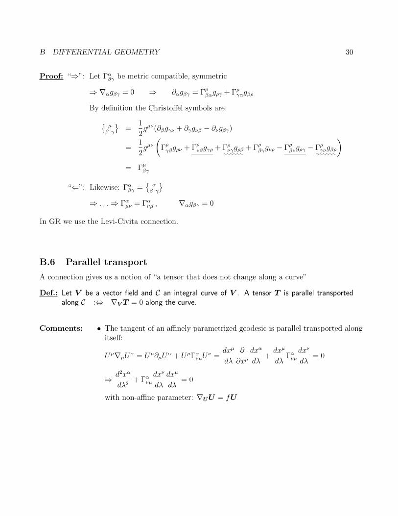
Proof: “⇒”: Let Γαβγ be metric compatible, symmetric
⇒ ∇αgβγ = 0 ⇒ ∂αgβγ = Γρβαgργ + Γργαgβρ
By definition the Christoffel symbols areµβ γ
=
1
2gµν(∂βgγν + ∂γgνβ − ∂νgβγ)
=1
2gµν(
Γργβgρν + Γρνβgγρ + Γρνγgρβ::::::
+ Γρβγgνρ − Γρβνgργ − Γργνgβρ::::::
)= Γµβγ
“⇐”: Likewise: Γαβγ =
αβ γ
⇒ . . .⇒ Γαµν = Γανµ , ∇αgβγ = 0
In GR we use the Levi-Civita connection.
B.6 Parallel transport
A connection gives us a notion of “a tensor that does not change along a curve”
Def.: Let V be a vector field and C an integral curve of V . A tensor T is parallel transportedalong C :⇔ ∇V T = 0 along the curve.
Comments: • The tangent of an affinely parametrized geodesic is parallel transported alongitself:
Uµ∇µUα = Uµ∂µU
α + UµΓανµUν =
dxµ
dλ
∂
∂xµdxα
dλ+dxµ
dλΓανµ
dxν
dλ= 0
⇒ d2xα
dλ2+ Γανµ
dxν
dλ
dxµ
dλ= 0
with non-affine parameter: ∇UU = fU

B DIFFERENTIAL GEOMETRY 31
• ∇V T = 0 determines T uniquely along the curve:
in coords. (xµ) the curve is xµ(λ)
⇒ V σ∇σTµν = V σ∂σT
µν + ΓµρσT
ρνV
σ − ΓρνσTµρV
σ
=d
dλT µν + ΓµρσT
ρνV
σ − ΓρνσTµρV
σ = 0
ODE theory ⇒ unique solution for all T µν
• parallel transport T along a curve from p to q
→ isomorphism between tensors at p, q
Unlike SR, this is path dependent in GR!
• Parallel transport preserves length of vectors:
d
dλ(WαW
α) = V µ∇µ(WαWα) = 2Wα V
µ∇µWα︸ ︷︷ ︸
=0
⇒ Geodesics do not change their timelike, spacelike or null character.
Def.: Acceleration along timelike curve: aµ ..= uρ∇ρuµ
The curve is a geodesic if aµ = 0 or aα = f uα
B.7 Normal coordinates
Def.: Let M be a manifold, Γ a connection, p ∈M.
“exponential map” : e : Tp →M , Xp 7→ q with
q ..= point a unit affine parameter distance along
geodesic through p with tangent Xp
Comments: 1) e can be shown to be one-to-one and onto locally
2) The vector Xp fixes the parametrization of the geodesic:
One can show that λXp , 0 ≤ λ ≤ 1 is mapped to point at
affine par. distance λ along the geodesic of Xp. (∗∗)

B DIFFERENTIAL GEOMETRY 32
Def.: Let eµ be a basis of Tp(M). “Normal coords. in nbhd. of p ∈M”:
coords. that assigns to q = e(X) ∈M the coordinates Xµ
Note: The coords. Xµ are not fixed by the vector X.
We still have the freedom to choose a basis for Tp(M).
Lemma: In normal coordinates, Γµ(νρ) = 0 at p.
If Γ is torsion free, then Γµνρ = 0.
Proof: From (∗∗) ⇒ affinely parametrized geodesic is given by
xµ(λ) = λXµp in normal coords.
⇒ geodesic eq.: 0 + Γµνρdxν
dλ
dxρ
dλ= ΓµνρX
νpX
ρp = 0 at p ∀X ∈ Tp(M)
⇒ Γµ(νρ) = 0
torsion free ⇒ Γµ[νρ] = 0 ⇒ Γµνρ = 0
Note: in general Γµνρ 6= 0 away from p !
Lemma: With Levi-Civita connection ⇒ in normal coords. at p: ∂ρgµν = 0
Proof: Γρµν = 0 ⇒ 2gσρΓρµν = ∂νgσµ + ∂µgνσ − ∂σgµν = 0
symmetrize on σ, µ, add ⇒ ∂νgσµ = 0
Lemma: Let (M, g) be a spacetime with LC connection
⇒ ∃ coordinates at p with: ∂ρgµν = 0 , gµν = ηµν = diag(−1, +1, +1, +1)
Proof: Choose an orthonormal basis eµ for Tp(M)
⇒ at p: X = X0e0 + . . .+X3e3 defines normal coords. xµ = Xµ
(∗∗) ⇒ point an affine par.distance along geodesic through p with
tangent e0 has coords. λ (e0)µ = (λ, 0, 0, 0)
⇒ The geodesic is xµ(λ) = (λ, 0, 0, 0)
In any coordinate system, the tangent to the curve (λ, 0, 0, 0) is ∂0 = ∂/∂x0
Likewise ∂µ = eµ ⇒ ∂µ is orthonormal ⇒ gµν = g(∂µ, ∂ν) = ηµν at p .
B DIFFERENTIAL GEOMETRY 33
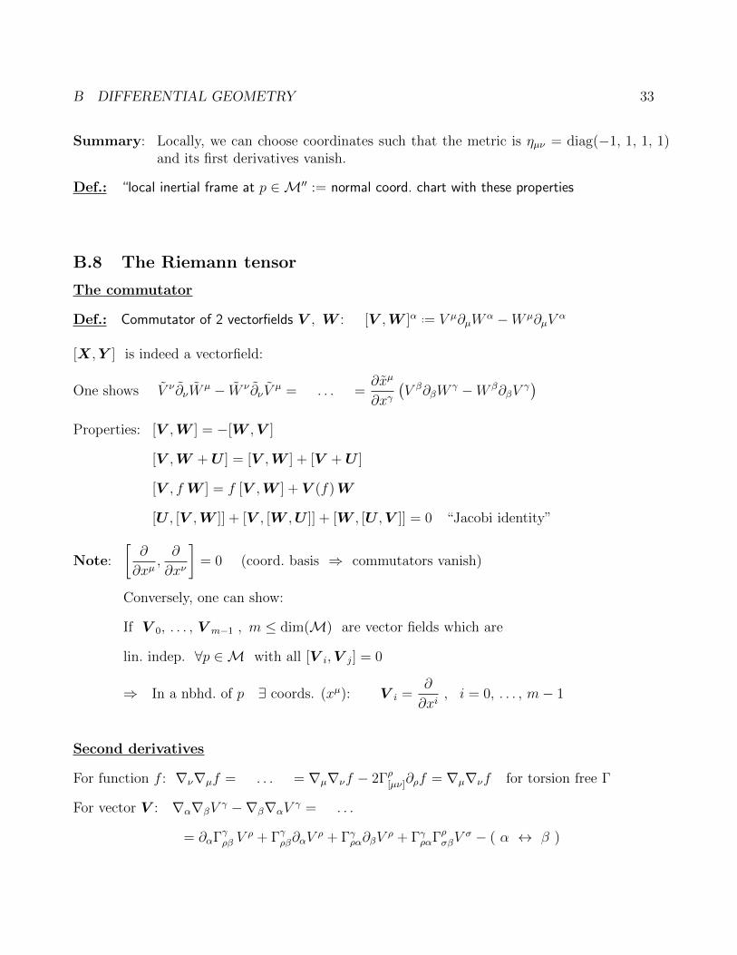
Summary: Locally, we can choose coordinates such that the metric is ηµν = diag(−1, 1, 1, 1)and its first derivatives vanish.
Def.: “local inertial frame at p ∈M′′ := normal coord. chart with these properties
B.8 The Riemann tensor
The commutator
Def.: Commutator of 2 vectorfields V , W : [V ,W ]α ..= V µ∂µWα −W µ∂µV
α
[X,Y ] is indeed a vectorfield:
One shows V ν ∂νWµ − W ν ∂νV
µ = . . . =∂xµ
∂xγ(V β∂βW
γ −W β∂βVγ)
Properties: [V ,W ] = −[W ,V ]
[V ,W +U ] = [V ,W ] + [V +U ]
[V , fW ] = f [V ,W ] + V (f)W
[U , [V ,W ]] + [V , [W ,U ]] + [W , [U ,V ]] = 0 “Jacobi identity”
Note:
[∂
∂xµ,∂
∂xν
]= 0 (coord. basis ⇒ commutators vanish)
Conversely, one can show:
If V 0, . . . , V m−1 , m ≤ dim(M) are vector fields which are
lin. indep. ∀p ∈M with all [V i,V j] = 0
⇒ In a nbhd. of p ∃ coords. (xµ): V i =∂
∂xi, i = 0, . . . , m− 1
Second derivatives
For function f : ∇ν∇µf = . . . = ∇µ∇νf − 2Γρ[µν]∂ρf = ∇µ∇νf for torsion free Γ
For vector V : ∇α∇βVγ −∇β∇αV
γ = . . .
= ∂αΓγρβ Vρ + Γγρβ∂αV
ρ + Γγρα∂βVρ + ΓγραΓρσβV
σ − ( α ↔ β )
B DIFFERENTIAL GEOMETRY 34
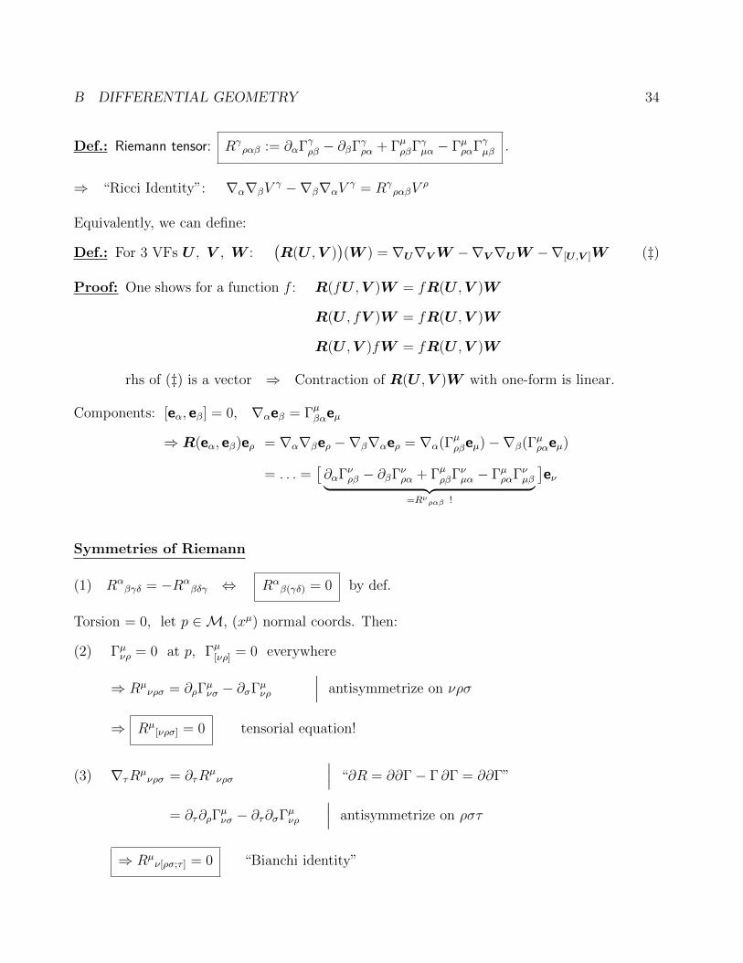
Def.: Riemann tensor: Rγραβ := ∂αΓγρβ − ∂βΓγρα + ΓµρβΓγµα − ΓµραΓγµβ .
⇒ “Ricci Identity”: ∇α∇βVγ −∇β∇αV
γ = RγραβV
ρ
Equivalently, we can define:
Def.: For 3 VFs U , V , W :(R(U ,V )
)(W ) = ∇U∇VW −∇V∇UW −∇[U ,V ]W (‡)
Proof: One shows for a function f : R(fU ,V )W = fR(U ,V )W
R(U , fV )W = fR(U ,V )W
R(U ,V )fW = fR(U ,V )W
rhs of (‡) is a vector ⇒ Contraction of R(U ,V )W with one-form is linear.
Components: [eα, eβ] = 0, ∇αeβ = Γµβαeµ
⇒ R(eα, eβ)eρ = ∇α∇βeρ −∇β∇αeρ = ∇α(Γµρβeµ)−∇β(Γµραeµ)
= . . . =[∂αΓνρβ − ∂βΓνρα + ΓµρβΓνµα − ΓµραΓνµβ︸ ︷︷ ︸
=Rνραβ !
]eν
Symmetries of Riemann
(1) Rαβγδ = −Rα
βδγ ⇔ Rαβ(γδ) = 0 by def.
Torsion = 0, let p ∈M, (xµ) normal coords. Then:
(2) Γµνρ = 0 at p, Γµ[νρ] = 0 everywhere
⇒ Rµνρσ = ∂ρΓ
µνσ − ∂σΓµνρ
∣∣∣ antisymmetrize on νρσ
⇒ Rµ[νρσ] = 0 tensorial equation!
(3) ∇τRµνρσ = ∂τR
µνρσ
∣∣∣ “∂R = ∂∂Γ− Γ ∂Γ = ∂∂Γ”
= ∂τ∂ρΓµνσ − ∂τ∂σΓµνρ
∣∣∣ antisymmetrize on ρστ
⇒ Rµν[ρσ;τ ] = 0 “Bianchi identity”

B DIFFERENTIAL GEOMETRY 35
(4) Levi-Civita connection, p ∈M ⇒ in normal coords.: ∂µgνρ = 0
⇒ 0 = ∂µδνρ = ∂µ(gνσgσρ) = gσρ∂µg
νσ∣∣∣ · gρτ
⇒ ∂µgντ = 0
⇒ ∂ρΓτνσ =
1
2gτµ(∂ρ∂σgµν + ∂ρ∂νgσµ − ∂ρ∂µgνσ
)⇒ Rµνρσ =
1
2
(∂ρ∂νgσµ + ∂σ∂µgνρ − ∂σ∂νgρµ − ∂ρ∂µgνσ
)+ “ΓΓ− ΓΓ”︸ ︷︷ ︸
=0
⇒ Rµνρσ = Rρσµν
It follows: Rαβγδ = −Rβαγδ
Parallel transport and curvature
Let X, Y be VFs with: lin. indep. everywhere and [X,Y ] = 0; let torsion = 0
⇒ we can choose coords. (s, t, . . .) such that X =∂
∂s, Y =
∂
∂t
Let p, q, r, u ∈M along integral curves of X, Y with coords.
(0, . . . , 0), (δs, 0, . . .), (δs, δt, 0, . . .), (0, δt, 0, . . .)
X
X
YY
p (0,0) δq ( s,0)
r ( s, t)δ δu (0, t)δ
Let Zp ∈ Tp(M) , parallel trapo Z along pqrup
to get Z ′p ∈ Tp(M)
⇒ limδs,δt→0
(Z ′p −Zp)α
δs δt= (Rα
βγδZβY γXδ)p
Proof: long script.

B DIFFERENTIAL GEOMETRY 36
Geodesic deviation
Goal: quantify relative acceleration of geodesics
Def.: Let (M,Γ) be a manifold with connection.
“1-parameter family of geodesics” := a map
γ : I × I ′ →M with I, I ′ ⊂ R, open and
(i) for fixed s, γ(s, t) is a geodesic with affine par. t
(ii) locally, (s, t) 7→ γ(s, t) is smooth, 1-to-1 has smooth inverse
⇒ the family of geodesics forms a 2-dim. surface Σ ⊂M
Let T be the tangent vector to γ(s = const, t) and S to γ(s, t = const)
In coords. (xµ): Sµ =dxµ
ds
⇒ xµ(s+ δs, t) = xµ(s, t) + δs Sµ(s, t) +O(δs2)
⇒ δsS points from one geodesic to a nearby one: “deviation vector”
⇒ “relative velocity” of nearby geodesics: ∇T (δsS) = δs∇TS
⇒ “relative acceleration” of nearby geodesics: δs∇T∇TSt=
s=
const
const
T
S
Theorem: ∇T∇TS = R(T ,S)T
⇔ T µ∇µ(T ν∇νSα) = Ra
λµνTλT µSν
Lemma: V µ∇µWα −W µ∇µV
α = V µ∂µWα + V µΓαρµW
ρ −W µ∂µVα −W µΓαρµV
ρ
= V µ∂µWα −W µ∂µV
α = [V ,W ]α
⇒ ∇VW −∇WV = [V ,W ]

B DIFFERENTIAL GEOMETRY 37
Proof: Use coords. (s, t) on Σ and extend to (s, t, . . .) in nbhd. of Σ
⇒ S =∂
∂s, T =
∂
∂t⇒ [S,T ] = 0
No torsion ⇒ ∇TS −∇ST = [T ,S] = 0
⇒ ∇T∇TS = ∇T∇ST = ∇S∇TT︸ ︷︷ ︸+R(T ,S)T 2
= 0 geodesic!
Comments: • Rαβγδ measures geodesic deviation; manifestation of curvature.
• Rαβγδ = 0⇔ relative acceleration = 0 for all families of geodesics.
• Tidal forces arise from geodesic deviation.
The Ricci tensor
Def.: The “Ricci tensor” is Rαβ..= Rµ
αµβ .
The “Ricci scalar” is R ..= gµνRµν .
The “Einstein tensor” is Gαβ −1
2gαβR .
Recall Bianchi Identity: Rαβ[γδ;µ] = 0∣∣∣ · gαγgβδ
⇒ 1
6gαγgβδ
[Rαβγδ;µ +Rαβδµ;γ +Rαβµγ;δ − Rαβδγ;µ︸ ︷︷ ︸
=−Rαβγδ;µ
−Rαβγµ;δ −Rαβµδ;γ
]= 0
⇒ 1
3gαγgβδ
[Rαβγδ;µ +Rαβδµ;γ +Rαβµγ;δ
]= 0
⇒ R;µ − gαγRαµ;γ − gβδRβµ;δ = 0
⇒ ∇µR− 2∇γRγµ = −2∇γ
(Rγµ −
1
2gγµR
)⇒ ∇µGµα = 0 “Contracted Bianchi Id.”

C PHYSICAL LAWS IN CURVED SPACETIMES 38
C Physical laws in curved spacetimes
Goal: How do we use differential geometry to describe physics?
C.1 The covariance principle
What we have so far:
• Equivalence principle: freely falling frame = inertial frame in SR
• Normal coordinates: ∃ coordinates: gαβ = ηαβ, Γαβγ = 0
• laws of SR invariant under Lorentz trafos
this motivates the
Covariance principle: The laws of GR are tensorial, i.e. coordinate invariant, and follow fromSR laws by replacing
(1) the metric: ηµν → gµν .
(2) the derivative: ∂ → ∇ .
Example: Electromagnetic field in SR:
Fµν = F[µν] with F0i = −Ei , Fij = εijkBk , (i, j, k = 1 . . . 3)
vacuum Maxwell eqs.: ηµν∂µFνρ = 0 , ∂[µFνρ] = 0
→ in GR: gαβ∇αFβγ = 0 , ∇[αFβγ] = 0
Note: Step SR → GR not unique since Rαβ = 0 in SR
C.2 The energy momentum tensor
Postulate: Mass-energy, stress in GR is described by the “energy momentum tensor” with
(1) Tαβ ..= flux of α momentum across a surface of constant xβ
(2) Tαβ = Tβα , ∇µTµν = 0
Interpretation: Tαβ = T (dxα,dxβ)
T 00 = 0 momentum across t = const = energy density
T i0 = xi momentum density
T 0i = energy flux across surface xi = const
T ij = flux of i momentum across xj = const

C PHYSICAL LAWS IN CURVED SPACETIMES 39
Tαβ often obtained from SR + covariance principle
Particles
1) in SR: Point like object with 4-momentum P µ = muµ = (E, P i)
4-velocity of observer in particle’s rest frame: wµ = (1, 0, 0, 0)
particle energy measured by this observer: E = −ηµνwµP ν
particle’s rest mass: ηµνPµP ν = −E2 + ~p 2 = −m2
2) in GR: Covariance ⇒ Pα = muα ⇒ gαβPαP β = −m2
Particle energy measured by observer: E = −gαβ(p) wα(p) P β(p)
works only if both are at p!electromagnetic field
1) pre-relativistic notation, Cartesian coordinates:
energy density: ρ =1
8π(EiEi +BiBi)
momentum density, energy flux: ji = 14πεijkEjBk “Poynting vector”
stress tensor: Sij =1
4π
[1
2(EkEk +BkBk)δij − EiEj −BiBj
]Maxwell eqs. ⇒ ∂ρ
∂t+ ∂iji = 0 ,
∂ji∂t
+ ∂jSij = 0
2) Special relativity:
Tµν =1
4π
(FµρFν
ρ − 1
4F ρσFρσηµν
)= Tνµ
T00 = ρ , T0i = −ji , Tij = Sij ; from 1)
Conservation: ∂µTµν = ηµσ∂σTµν = 0
3) GR: Tαβ =1
4π
(FαµFβ
µ − 1
4F µνFµνgαβ
)with ∇µTµα = 0

C PHYSICAL LAWS IN CURVED SPACETIMES 40
Dust
Continuum limit of non-interacting particles of rest mass m and number density n
⇒ Particles are freely falling!
In comoving frame: uµ = [1, 0, 0, 0], locally gαβ = ηαβ
⇒ ρ = mn , T i0 = T 0j = 0 , T ij = 0
⇒ Tαβ = ρuαuβ = mnuαuβ .
Perfect fluids
Def.: Continuous matter with (1) no heat conduction, (2) no viscosity in locally comovingframe.
(1) = energy can only flow if the particles flow.
(2) = Force between particles only has radial component.
⇒ For particles on xi axis, only pi momentum can flow.
⇒ T ij 6= 0 only for i = j.
No direction preferred ⇒ T 11 = T 22 = T 33 =.. P
In SR: In comoving frame Tαβ = diag(ρ, P, P, P ) ; uα = (1, 0, 0, 0) , gαβ = ηαβ
⇒ Tαβ = (ρ+ P )uαβ + Pηαβ
Covariance principle ⇒ Tαβ = (ρ+ P )uαuβ + Pgαβ
Conservation ∇αTαβ = 0
⇒ uα∇αρ+ (ρ+ P )∇αuα = 0
(ρ+ P )uα∇αuβ = −(gαβ + uαuβ)∇αP GR’s version of Euler equation
Comments: • We still need an equation of state describing the matter. E.g. polytrope P ∝ ρΓ
• P = 0 ⇒ fluid moves on geodesics

C PHYSICAL LAWS IN CURVED SPACETIMES 41
C.3 The Einstein equations
Postulates of GR
(1) Spacetime is a 4-dim. Lorentzian manifold with metric and Levi-Civita connection.
(2) Free particles follow timelike or null geodesics.
(3) Energy, momentum and stress of matter is described by a symmetric,
conserved tensor Tαβ : ∇αTαβ = 0 .
(4) Curvature is related to matter by the Einstein eqs.
Gαβ = Rαβ −1
2gαβR =
8πG
c4Tαβ ; G = Newton’s constant
Comments: • Factor8πG
c4from Newtonian limit (cf. below)
• Vacuum ⇒ Gαβ = Rαβ −1
2gαβ R = 0
∣∣∣ · gαβ⇒ R = 0 ⇒ Rαβ = 0
• G = 8πT represents 10 coupled, non-linear PDEs. Hard to solve!
Theorem: (Lovelock 1972) Let Hαβ be a symmetric tensor with
(i) in any coords. Hµν = Hµν(gµν , ∂ρgµν , ∂σ∂ρgµν) at every p ∈M
(ii) ∇αHαβ = 0
(iii) Hµν linear in ∂σ∂ρgµν
⇒ ∃A,B∈R Hαβ = AGαβ +B gαβ
⇒ we can modify Einstein’s eqs.: Gαβ + Λgαβ =8πG
c4Tαβ
Λ = Cosmological constant
Λgαβ is equivalent to perfect fluid with ρ = −P =Λc4
8πG
D THE SCHWARZSCHILD SOLUTION AND CLASSIC TESTS OF GR 42
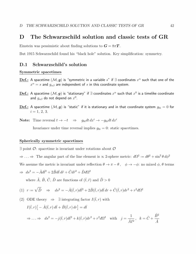
D The Schwarzschild solution and classic tests of GR
Einstein was pessimistic about finding solutions to G = 8πT .
But 1915 Schwarzschild found his “black hole” solution. Key simplification: symmetry.
D.1 Schwarzschild’s solution
Symmetric spacetimes
Def.: A spacetime (M, g) is “symmetric in a variable s” if ∃ coordinates xα such that one of thexα = s and gαβ are independent of s in this coordinate system.
Def.: A spacetime (M, g) is “stationary” if ∃ coordinates xα such that x0 is a timelike coordinateand gαβ do not depend on x0.
Def.: A spacetime (M, g) is “static” if it is stationary and in that coordinate system g0i = 0 fori = 1, 2, 3.
Note: Time reversal t→ −t ⇒ g0idt dxi → −g0idt dx
i
Invariance under time reversal implies g0i = 0: static spacetimes.
Spherically symmetric spacetimes
∃ point O: spacetime is invariant under rotations about O
⇒ . . .⇒ The angular part of the line element is ∝ 2-sphere metric: dΩ2 ..= dθ2 + sin2 θ dφ2
We assume the metric is invariant under reflection θ → π− θ , φ→ −φ: no mixed φ, θ terms
⇒ ds2 = −Adt2 + 2Bdt dr + Cdr2 + DdΩ2
where A, B, C, D are functions of (t, r) and D > 0
(1) r ..=√D ⇒ ds2 = −A(t, r)dt2 + 2B(t, r)dt dr + C(t, r)dr2 + r2dΩ2
(2) ODE theory ⇒ ∃ integrating factor I(t, r) with
I(t, r)[− A(t, r) dt+ B(t, r) dr
]= dt
⇒ . . .⇒ ds2 = −j(t, r)dt2 + k(t, r)dr2 + r2dΩ2 with j =1
AI2, k = C +
B2
A

D THE SCHWARZSCHILD SOLUTION AND CLASSIC TESTS OF GR 43
(3) Now Einstein eqs.: Rtr =
∂tk
k2r= 0 ⇒ k = k(r)
Rtt =
r2∂rk + k2 − kk2r2
= 0 ⇒ . . .⇒ k =r
r − 2M, M = const
Rrr =−r∂rj + jk − j−jkr2
= 0 ⇒ j =r − 2M
rf(t)
(4) signature +2 ⇒ f(t) > 0
Rescale t such that√f(t)dt = dt
⇒ ds2 = −(
1− 2M
r
)dt2 +
(1− 2M
r
)−1
dr2 + r2(dθ2 + sin2 θ dφ2) (†)
Comments: • (†) = unique solution in spherical symmetry and vacuum. It is static!
• limr→∞
gαβ = ηαβ: asymptotic flatness
• M can be shown to be the mass-energy of the spacetime.
• (†) also describes the spacetime exterior to spherically symmetric stars.
⇒ Birkhoff’s Theorem: Any spherically symmetric solution of the vacuum Einstein equations isgiven by the Schwarzschild metric. It is static and asymptotically flat.
D.2 Geodesics in the Schwarzschild spacetime
L = −(
1− 2M
r
)t2 +
(1− 2M
r
)−1
r2 + r2θ2 + r2 sin2 θ φ2
θ component: ⇒ d
dλ
(∂L∂θ
)− ∂L∂θ
= 2r2θ + 4rrθ − 2r2 sin θ cos θ φ2 = 0
⇒ θ + 2rθ
r− sin θ cos θ φ2 = 0
Rotate coordinates such that θ = π/2 , θ = 0 at λ0
⇒ θ = π/2 always WLoG!

D THE SCHWARZSCHILD SOLUTION AND CLASSIC TESTS OF GR 44
Noether⇒ (i)∂L∂t
= 0 ⇒ E = −1
2
∂L∂t
=
(1− 2M
r
)t = const
(ii)∂L∂φ
= 0 ⇒ L =1
2
∂L∂φ
= r2 sin2 θ φ = r2φ = const
(iii)∂L∂λ
= 0 ⇒ Q = −(
1− 2M
r
)t2 +
(1− 2M
r
)−1
r2 + r2φ2 =
−1 timelike
0 null
1 spacelike
Meaning of E, L: Consider r M ⇒ gαβ → ηαβ ⇒ SR
E: for timelike geodesics with λ = τ : E =dt
dτ= γ
⇒ Em = mγ ⇒ E = energy per rest mass m
L: Likewise Lm = mr2φ = mγr2dφ
dt= angular momentum per rest mass
Plug E, L into Eq. for Q
⇒ −E2 + r2 +1
r2
(1− 2M
r
)L2 =
(1− 2M
r
)Q
⇒ 1
2r2 + V (r) =
1
2E2 , V (r) =
1
2
(1− 2M
r
) (L2
r2−Q
)(‡)
Comparison with Newtonian equations
Energy balance for particle in Newtonian gravity
Ekin =1
2mr2 +
1
2mr2φ2 =
1
2mr2 +
m
2
L2
r2
Epot = −GMm
r, Let’s set G = 1
⇒ 1
2mr2 +
1
2mL2
r2− Mm
r= Ekin + Epot = const
Comparison with (‡) forQ = −1: (1) (E2 − 1)m/2 = Ekin + Epot
(2) GR has extra term −ML2
r3

D THE SCHWARZSCHILD SOLUTION AND CLASSIC TESTS OF GR 45
Summary:1
2r2 + VN/GR(r) = const . VN(r) =
1
2
L2
r2− M
r
VGR(r) =1
2
L2
r2+Q
M
r− ML2
r3
Effective potential V determines trajectories
Newtonian: For L 6= 0: limr→0
V =∞ , limr→∞
V = 0
Extrema from: V ′N(r) = −L2
r3+M
r2= 0 ⇒ r =
L2
M
V ′′N(r) =3L2
r4− 2M
r3⇒ V ′′N(L2/M) = M4/L6 > 0
⇒ circular orbit at r =L2
M
VN min. ⇒ orbit stable
0 5 10
r / M
-2
-1
0
1
2
3
4
VN
L / M = 0
L / M = 1
L / M = 2
L / M = 4
L / M = 8
Newtonian

D THE SCHWARZSCHILD SOLUTION AND CLASSIC TESTS OF GR 46
GR null: limr→0
V = −∞ , limr→∞
V = 0
Extrema: V ′GR(r) = −L2
r3+ 3
ML2
r4= 0 ⇒ r = 3M
V ′′GR(r) =3L2
r4− 12ML2
r5⇒ V ′′GR(3M) = − L2
81M4< 0
⇒ circular orbit at r = 3M
VGR max. ⇒ orbit unstable
0 5 10
r / M
-4
-3
-2
-1
0
1
2
VGR
L / M = 1L / M = 2L / M = 4L / M = 8
GR null geodesics
GR timelike: limr→0
V = −∞ , limr→∞
V = 0
Extrema: r = r± =L2
2M±√
L4
4M2− 3L2 > 0 for L2 > 12 M2
For L2 > 12 M2 : V ′′GR(r+) > 0 , V ′′GR(r−) < 0
⇒ stable circular orbit at r+
⇒ unstable circular orbit at r−
0 5 10
r / M
-4
-3
-2
-1
0
1
2
VGR
L / M = 0L / M = 1L / M = 2
L2 / M
2 = 12
L / M = 4L / M = 8
GR timelike geodesics
0 5 10 15 20
r / M
-0.1
-0.05
0

D THE SCHWARZSCHILD SOLUTION AND CLASSIC TESTS OF GR 47
D.3 Classic tests of GR
Mercury’s perihelion precession
Newtonian:1
2mr2 +
1
2mL2
r2− Mm
r=.. E (†)
φ = L/r2 ⇒ φ(t) monotonic → parametrize orbit with φ
y ..=1
r⇒ . . .⇒ r ..=
dr
dt= −Ldy
dφ=.. −Ly′
(†) ⇒ (y′)2L2 + L2y2 − 2My = 2E∣∣∣ d
dφ
⇒ 2L2y′y′′ + 2L2yy′ − 2My′ = 0
⇒ y′ = 0 ∨ y′′ + y =M
L2
⇒ y =M
L2(1 + ε cosφ) Keppler ellipse for ε < 1: No perihelion precession
GR: Use again y(φ), Q = −1
⇒ . . .⇒ L2(y′)2 + L2y2 − 2My − 2ML2y3 = E2 − 1∣∣∣ d
dφ
⇒ y′′ + y =M
L2+ 3My2
Expand solution in α ..= 3M2
L2∼ O(10−7) for Mercury
⇒ y = y0 + αy1 +O(α2)
⇒ y′′0 + y0 −M
L2+ α
(y′′1 + y1 −
L2
My2
0
)+O(α2) = 0
Order α0: y′′0 + y0 −M
L2= 0 ⇒ y0 =
M
L2(1 + ε cosφ) Newtonian case!
Order α1: Plug in y0 and use cos2 φ = (1 + cos 2φ)/2
⇒ y′′1 + y1 =M
L2
(1 +
ε2
2
)+
2M
L2ε cosφ+
M
2L2ε2 cos 2φ
Ansatz: y1 = A+Bφ sinφ+ C cos 2φ
⇒ . . . ⇒ A =M
L2
(1 +
ε2
2
), B =
Mε
L2, C = −Mε2
6L2.

D THE SCHWARZSCHILD SOLUTION AND CLASSIC TESTS OF GR 48
Solution: y = y0 + αy1 =M
L2(1 + ε cosφ) + α
M
L2
[1 + εφ sinφ+ ε2
(1
2− 1
6cos 2φ
)]Ignore last term ∝ ε2
⇒ y ≈ M
L2(1 + α + ε cosφ+ αεφ sinφ)
α 1 ⇒ cos(φ− αφ) = cosφ cosαφ+ sinφ sinαφ ≈ cosφ+ αφ sinφ
⇒ y ≈ M
L21 + α + ε cos[φ(1− α)]
Key result: y returns to the same value as (1− α)φ increases by 2π
⇒ Perihelion period: φn+1 − φn =2π
1− α ≈ 2π(1 + α) = 2π
(1 +
3M2
L2
)Circular timelike geodesic ⇒ r = r+ ⇒ . . .⇒ L2 =
Mr
1− 3M/r≈Mr
⇒ ∆φ ≈ 6πM
r=
43′′
century
Light bending
1) Newtonian
Without gravitational field: y′′ + y = 0 ⇒ y =1
bsinφ , straight line
φ2
r2r1b φ1
light from left (φ = π) to right (φ = 0); b = impact parameter

D THE SCHWARZSCHILD SOLUTION AND CLASSIC TESTS OF GR 49
With field: Recall y =M
L2(1 + ε sinφ) , we shifted Phase: cos → sin
Small deflection ⇒ y = 0 at φ = −∆φ, π + ∆φ with ∆φ 1
⇒ sin(−∆φ) ≈ −∆φ = −1
ε, sin(π + ∆φ) ≈ −∆φ = −1
ε
It follows:1
ε 1 ⇒ ε 1
Impact parameter1
b= y(π/2) =
M
L2(1 + ε) ≈ M
L2ε
Angular momentum: mL = |~r × ~p| = bmc = bm ⇒ L = b
Total deflection 2∆φ =2
ε=
2M
b
bφ
π +∆φ
−∆φ
r
2) GR
Geodesic equation forQ = 0: L2(y′)2 + L2y2 − 2ML2y3 = E2∣∣∣ d
dφ
⇒ y′′ + y = 3My2
Without field: M = 0 ⇒ y′′0 + y0 = 0 ⇒ y0 =1
bsinφ (like Newtonian)
Small deflection: perturb around straightline y0 = (sinφ)/b
⇒ y = y0 +M
b∆y +O(M2/b2)
⇒ . . .⇒ ∆y′′ + ∆y =3
b
1− cos 2φ
2

D THE SCHWARZSCHILD SOLUTION AND CLASSIC TESTS OF GR 50
Homogeneous DE: ∆y′′ + ∆y = 0 solved by ∆y = A cosφ+B sinφ
Particular solution: ∆y =1
2b(3 + cos 2φ)
With A =2
b, B = 0, we get y = 0 for φ→ π
⇒ y = y0 +M
b∆y =
1
bsinφ+
M
2b2(3 + cos 2φ) +
2M
b2cosφ
Deflection δφ from y = 0 at φ = 0 + δφ
⇒ 0 ≈ δφ
b+M
2b2(3 + 1) +
2M
b2
⇒ δφ ≈ −4M
b
For sun: M = 1.5 km, b ≈ R = 7× 10⁵ km: |δφ| ≈ 1.77′′
Measured by Eddington expedition in 1919.
Shapiro time delay
Radio signal past sun to Venus and back. Measure time delay.
1) Without field: Pythagoras ⇒ T = 2(√
r21 − b2 +
√r2
2 − b2)
Venus Earthr1 r
2
b
Sun
2) With field
Null geodesic (Q=0): r2 +
(1− 2M
r
)L2
r2= E2 , t =
(1− 2M
r
)−1
E
⇒ . . .⇒ dr
dt= ±
(1− 2M
r
)√1−
(1− 2M
r
)L2
r2E2
D THE SCHWARZSCHILD SOLUTION AND CLASSIC TESTS OF GR 51
At point of closest approach: r = b , dr/dt = 0
⇒(
1− 2M
b
)L2
b2E2= 1 ⇒ L2
E2=
b2
1− 2Mb
eliminates L, E
⇒ T = 2
∫ r1
b
dr
f(r)+ 2
∫ r2
b
dr
f(r), f(r) =
(1− 2M
r
)√1− b2
r2
1− 2M/r
1− 2M/b
Solve integral by Taylor expanding f(r) in M/r using M/b 1
⇒ . . .⇒ T ≈ 2
(√r2
1 − b2 +√r2
2 − b2
)︸ ︷︷ ︸
=..TMink
+4M
(lnr1 +
√r2
1 − b2
b+ ln
r2 +√r2
2 − b2
b
)
+2M
(√r1 − br1 + b
+
√r2 − br2 + b
).
For Venus and Earth: ∆T ≈ 77 km = 257 µs
D.4 The causal structure of the Schwarzschild spacetime
Recall Schwarzschild: ds2 = −(
1− 2M
r
)dt2 +
(1− 2M
r
)−1
dr2 + r2(dθ2 + sin2 θ dφ2)
singular at r = 0, r = 2M ; what’s happening?
Light cones
Timelike (null) curves travel inside (on) light cones
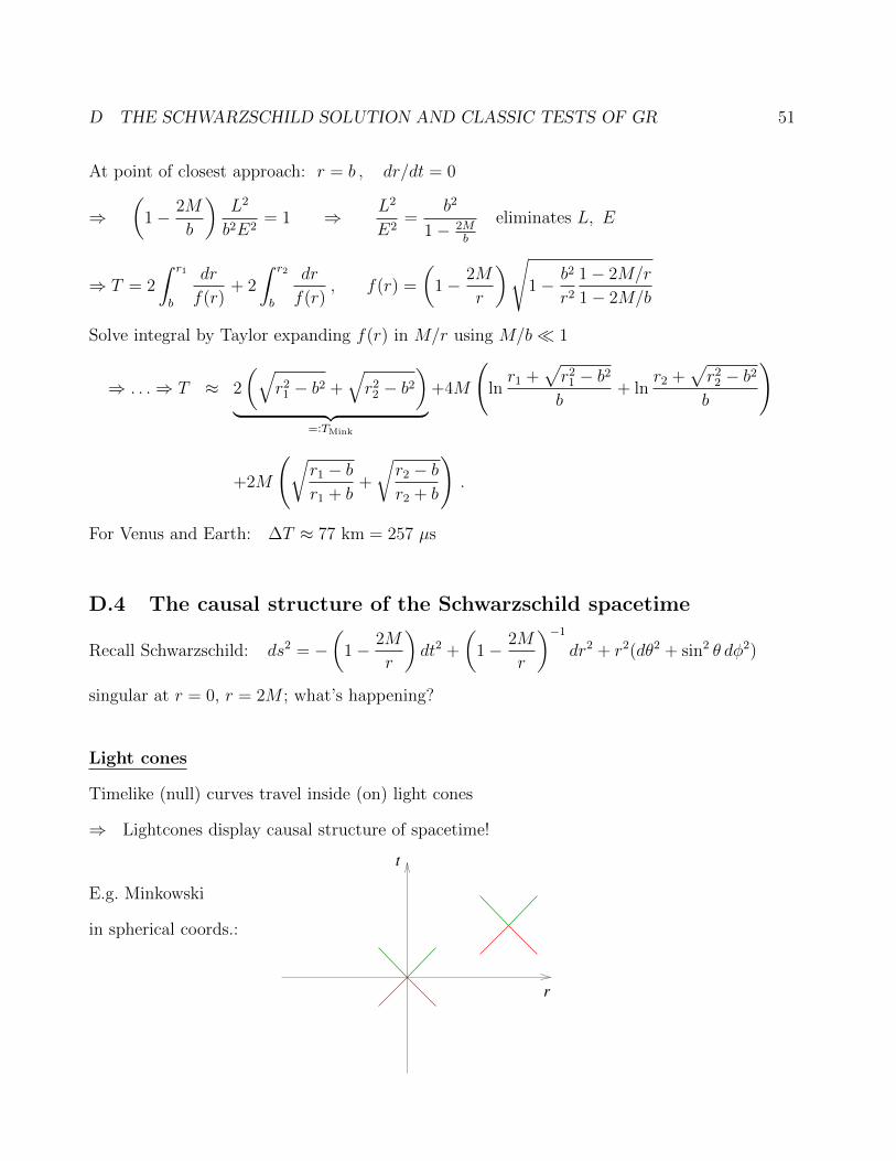
⇒ Lightcones display causal structure of spacetime!
E.g. Minkowski
in spherical coords.:
r
t

D THE SCHWARZSCHILD SOLUTION AND CLASSIC TESTS OF GR 52
Radial null geodesics: dθ = dφ = 0; Let λ be an affine parameter
t component: We already know
(1− 2M
r
)t = E = const
r component: EL eqs.:d
dλ
∂L∂r
=∂L∂r
⇒ . . .⇒(
1− 2M
r
)r2
Mr = r2 − E2
Solved by r = ±E
⇒ r = ±Eλ+ r0 is also an affine parameter. Let’s use r.
⇒ dt
dr=t
r= ± r
r − 2M
⇒ . . .⇒ t(r) = ±(r + 2M ln |r − 2M |) + k , k = const
0 2M 4M
r
0
5M
10M
t
r > 2M : In/Outgoing null geodesics for the +/− sign.
Note: r = const timelike (inside light cone)
r < 2M : ds2 = −(
2M
r− 1
)−1
dr2 +
(2M
r− 1
)dt2
⇒ grr < 0 , gtt > 0 ⇒ r is the timelike coordinate, t spacelike
Light cones tilted horizontally, but In/Outgoing direction unclear.

D THE SCHWARZSCHILD SOLUTION AND CLASSIC TESTS OF GR 53
Infalling observers
Consider timelike geodesic starting at large r:(1− 2M
r
)t = E , −
(1− 2M
r
)t2 +
(1− 2M
r
)−1
r2 = Q = −1
⇒ −E2 + r2 = −1 +2M
r
Observer starting at rest at r →∞ ⇒ E = 1 (cf. Sec. D.2)
Use proper time: r2 =2M
r⇒ dτ
dr= −
√r
2M< 0 infalling!
⇒ . . .⇒ τ − τ0 =2
3√
2M
(r
3/20 − r3/2
)How about coordinate time t?
dt
dr=t
r= −
√r
2M
(1− 2M
r
)−1
⇒ . . .⇒ t−t0 = − 2
3√
2M
[r3/2 − r3/2
0 + 6M(√r −√r0)
]+2M ln
(√r +√
2M)(√
r0 −√
2M)
(√r0 +
√2M)(√
r −√
2M)
0 5 10 15 20
r / M
0
10
20
30
40
50
60
70
τ(r)
t(r)
Interpretation: • t = proper time of observer at infinity
• geodesic crosses r = 2M at finite τ but t→∞
• one falls in finite time, but process infinitely redshifted for outside observer
D THE SCHWARZSCHILD SOLUTION AND CLASSIC TESTS OF GR 54
Ingoing Eddington Finkelstein (IEF) coordinates
Ingoing null geodesics: t+ 2M ln |r − 2M | = −r + const
New time coordinate: t = t+ 2M ln |r − 2M | ⇒ dt = dt+2M
r − 2Mdr
⇒ . . .⇒ ds2 = −(
1− 2M
r
)dt2 +
4M
rdtdr +
(1 +
2M
r
)dr2 + r2(dθ2 + sin2 θ dφ)
Ingoing geodesics: t = −r + const
Outgoing geodesics: t = r + 4M ln |r − 2M |+ const
0 2M 10M
r
0
5M
10M
t
Light cones tilt over inwards at r = 2M .
Def.: Event horizon: The outermost boundary of a region of spacetime from which no null geodesicsor timelike curves can escape to infinity.
Israel’s theorem: If a spacetime is static, asymptotically flat and contains a regular horizon thenit is a Schwarzschild spacetime.
We can use a null coordinate v = t+ r ⇒ dt = dv − dr
⇒ . . .⇒ ds2 = −(
1− 2M
r
)dv2 + 2dr dv + r2dΩ2
Note: ∂r is tangent to curves v = const. Clearly g(∂r, ∂r) = 0.

D THE SCHWARZSCHILD SOLUTION AND CLASSIC TESTS OF GR 55
Outgoing Eddington Finkelstein (OEF) coordinates
Outgoing null geodesics: t− 2M ln |r − 2M | = r + const
New time coordinate: t = t− 2M ln |r − 2M | ⇒ dt = dt− 2M
r − 2Mdr
⇒ . . .⇒ ds2 = −(
1− 2M
r
)dt2 − 4M
rdtdr +
(1 +
2M
r
)dr2 + r2(dθ2 + sin2 θ dφ) (∗)
We can use a null coordinate u = t− r ⇒ dt = du+ dr
⇒ . . .⇒ ds2 = −(
1− 2M
r
)du2 − 2dr du+ r2dΩ2
Ingoing geodesics: t = −r − 4M ln |r − 2M |+ const
Outgoing geodesics: t = r + const
0 2M 10M
r
0
5M
10M
t
Now all light cones point outwards.
But above we showed that light cones point inwards at r < 2M . WTF?!?
On the other hand: Schwarzschild should be time symmetric. What’s going on?
D THE SCHWARZSCHILD SOLUTION AND CLASSIC TESTS OF GR 56
Kruskal-Szekeres coordinates
Step 1: Combine IEF and OEF: v = t+ r + 2M ln
(r − 2M
r∗
); r∗: integration constant
u = t− r − 2M ln
(r − 2M
r∗
)
⇒ ds2 = −(
1− 2M
r
)du dv + r2dΩ2
Step 2: Use an exponential version of u, v:
v = ev
4M , u = −e− u4M
⇒ uv = −e v−u4M = −r − 2M
r∗e
r2M
⇒ . . .⇒ ds2 = −16M2
r/r∗e−
r2M du dv + r2dΩ2
Step 3: Go back to time and radius:
t =1
2(v + u) , r =
1
2(v − u)
⇒ . . .⇒ ds2 =16M2
r/r∗e−
r2M (−dt2 + dr2) + r2dΩ2 , from now on set r∗ = 1
r implicitly given through t2 − r2 = −e r2M (r − 2M)
Comments: • Metric regular at r = 2M
• Radial null geodesics are: t = ±r + const
• Coordinate range:
a) r = 2M ⇒ t2 − r2 = 0 ⇒ t = ±r
b) r = 0 ⇒ t2 − r2 = 2M ⇒ t = ±√r2 + 2M
c) t2 − r2 = −er/(2M)(r − 2M) monotonically decreasing in r
⇒ t2 − r2 < 2M for all r > 0
d) No further restrictions on t, r: r ∈ (−∞,∞) , t2 ≤ r2 + 2M

D THE SCHWARZSCHILD SOLUTION AND CLASSIC TESTS OF GR 57
Kruskal diagram
(1) Curves r = r0: t2 − r2 = −e r02M (r0 − 2M) =.. C
⇒ t = ±√r2 + C
(2) Curves t = t0: t =1
2(v + u) =
√r − 2Me
r4M sinh
t
4M
r =1
2(v − u) =
√r − 2Me
r4M cosh
t
4M
⇒ tanht
4M=t
r
-4 -2 0 2 4
r
-4
-2
0
2
4t
r=3M
r=0
r=2.5Mr=3M r=2.5M
r=2M r=2M
r=1.8M
r=1.5M
r=1.8M
r=1.5M
r=0
t=-2M
t=-M
t=M
t=2M
Comments: • Spacetime extended: white hole, black hole, 2 asymptotically flat regions
• Resolves puzzle of light cones in IEF/OEF coordinates.

D THE SCHWARZSCHILD SOLUTION AND CLASSIC TESTS OF GR 58
D.5 Hawking radiation
GR is a classical theory and we do not yet have a quantum theory of gravity.
Semi-classical calculations: QM on curved background spacetime.
Hawking effect: Pair creation of virtual particles
→ one falls into black hole; the other escapes
Hawking radiation depends on temperature T =~c3
8πGMkB
− 1
A
dM
dt= σT 4 , σ =
π2k4B
60~3c2
⇒ dM
dt= − ~c6
15360π G2M2⇒ t = 5120
πG2
~c6M3 ; for M : t = O(1060) yr
Note: Energy loss → higher T → more radiation!

E COSMOLOGY 59
E Cosmology
Goal: Simplified model of the entire universe.
E.1 Homogeneity and isotropy
Observations: • Electromagnetic observations of universe out to ∼ 1011 pc.
• Galaxies have R ∼ 105 km → point like on scale 1011 pc.
• On scales ∼ 109 pc, the universe looks the same on average and the samein every direction.
• Hubble redshift → universe seems to expand.
⇒ Model universe as an isotropic, spatially homogeneous spacetime with fluid matter.
Cosmological principle: At a given time, the universe is spatially homogeneous and isotropicwhen viewed on large scales.
Weyl’s postulate: The world lines of the universe’s fluid elements are orthogonal to hypersurfacesof constant time, Σt, to which the cosmological principle applies.
Comments: • Isotropy is observer dependent: a boosted observer will not see isotropy.
• Which observer sees isotropy? The one comoving with the cosmological fluid.
• We do not require homogeneity in time!
Adapted coordinates
Let xi be spatial coordinates comoving with the cosmological fluid.
Let t be proper time along the world lines of observers comoving with the fluid.
Isotropy ⇒ no spatial metric component has a prefered time dependency
⇒ ds2 = −dt2 + g0idt dxi + a(t)2hij(x
k)dxi dxj .
Consider basis e0 = ∂t, ei = ∂i
⇒ e0 = four-velocity of comoving observers and ei are tangent to Σt
By Weyl’s postulate, e0 is orthogonal to Σt, i.e. to the ei
⇒ g0i = g(e0, ei) = 0

E COSMOLOGY 60
⇒ ds2 = −dt2 + a(t)2hij(xk)dxi dxj (†)
Note: Observers moving relative to the fluid do not move orthogonally to Σt.
⇒ g0i 6= 0 ⇒ this observer does not see isotropy.
Recall: Spatial part of spherically symmetric metric: d`2 = C(t, r)dr2 +D(t, r)dΩ2 (‡)
Spherical symmetry = isotropy around one point
Isotropy around every point = “Maximal symmetry” = Spherical symmetry + more
⇒ we can combine (†) and (‡)
⇒ factorize C(t, r) = a(t)2e2β(r) , D(t, r) = a2(t)r2 ⇒ d`2 = a2(t)[e2β(r)dr2 + r2dΩ2
]Next use our differential geometry on the hypersurface t = const
3-dimensional Ricci scalar R = Rii , i = 1, 2, 3
Spatial homogeneity ⇒ R = . . . =2
r2
[1− ∂r(re−2β)
]= const =.. k
⇒ e2β =1
1− 16kr2 − A
r
No conical singularity ⇒ limr→0
d`2 ∝ (dr2 + r2dΩ2) ⇒ A = 0
⇒ Robertson-Walker metric: ds2 = −dt2 + a(t)2
[dr2
1− kr2+ r2(dθ2 + sin2 θ dφ2)
]Note: We can always rescale r, a so that k = +1, 0 or −1
1) k = 0 : d`2 = dr2 + r2dΩ2 = dx2 + dy2 + dz2
Flat metric on R3; k = 0 models are called flat.
2) k = +1: r = sinχ ⇒ d`2 = dχ2 + sin2 χdΩ2
Metric on a 3-sphere (w2 + x2 + y2 + z2 = r2 in R4); closed models
3) k = −1: r = sinhψ ⇒ d`2 = dψ2 + sinh2 ψdΩ2
Metric of a “saddle”; open models
E COSMOLOGY 61
E.2 The Friedmann equations
The matter fields
Recall: Perfect fluids are isotropic by definition!
We therefore set Tµν = (ρ+ P )uµuν + Pgµν
Comoving frame: uµ = (1, 0, 0, 0) ⇒ T µν = diag(−ρ, P, P, P )
⇒ T = T µµ = −ρ+ 3P coordinate invariant!
Conservation: ∇µTµν = 0 ⇒ . . .⇒ ρ = −3
a
a(ρ+ P )
Equation of state: Cosmological matter typically has P = wρ , w = const
⇒ ρ
ρ= −3(1 + w)
a
a⇒ ρ ∝ a−3(1+w)
(1) Dust
w = 0 ⇒ P = 0 ⇒ ρ ∝ a−3
Pressure between galaxies ≈ 0.
(2) Radiation
Statistical Physics: photons are a gas with P = ρ/3
⇒ w =1
3⇒ ρ ∝ a−4
Fourth power of a comes from redshift (cf. below).
(3) Dark energy
Recall Lovelock’s theorem: We can add Λgαβ to the Einstein equations.
Perfect fluid with w = −1: 8πTµν = 8πPgµν!
= −Λgµν ⇒ − P = ρ =Λ
8π
w = −1 ⇒ ρ ∝ a0
Interpretation: Non-zero of the vacuum. Density = const, independent of volume
Do not confuse with dark matter!
E COSMOLOGY 62
Def.: H :=a
ais the Hubble parameter.
q := −aaa2
is the deceleration parameter.
ρcrit :=3H2
8πis the critical density; its significance will be revealed below.
Ω =ρ
ρcrit
=8π
3H2ρ is the density parameter.
Note: These are time dependent variables. The “parameters” are their present day values.
The Einstein equations
Plug Robertson-Walker metric into Gαβ + Λgαβ = 8πTαβ
⇒ . . .⇒ 3a2 + k
a2− Λ = 8πρ (I) ,
2aa+ a2 + k
a2− Λ = −8πP (II)
a
a= −4π
3(ρ+ 3P ) +
Λ
3(III)
Note: Eq. (III) follows from (I), (II) but can be useful.
Differentiate (I) and combined with (I), (II)
⇒ . . .⇒ ρ+ 3a
a(ρ+ P ) = 0
∣∣∣ · a3
⇒ d
dt(a3ρ) + P
d
dta3 = 0
Volume V ∝ a3, energy E = V ρ, so this can be written as dE + PdV = 0
E.3 Cosmological redshift
Radial null curves: ds2 = −dt2 +a2
1− kr2dr2 = 0 ⇒ dt
a(t)= ± dr√
1− kr2
A galaxy at r = R emits at times te and te + ∆te.
These reach an observer at r = 0 at times to, to + ∆to.

E COSMOLOGY 63
⇒∫ to
te
dt
a= −
∫ 0
R
dr√1− kr2
=
∫ to+∆to
te+∆te
dt
a
(‘−’ since ingoing geodesic)
⇒∫ to+∆to
to
dt
a=
∫ te+∆te
te
dt
a
r=0 r=R
t
E.g. crests of light wave: ∆te, ∆to to − te ⇒ a ≈ const
⇒ ∆toa(to)
=∆tea(te)
⇒ λoλe
=a(to)
a(te)
Nearby galaxies: Taylor expand a(te) ≈ a(to)− (to − te)a(to)
⇒ a(to)
a(te)≈ 1 + (to − te)
a(to)
a(to)= 1 + (to − te)H(to)
Hubble’s law with distance = c(to − te) , c = 1.
Luminosity distance: Surface of constant radius, time: ds2 = a(t)2r2(dθ2 + sin2 θ dφ2)
Area of sphere of constant r: 4πa2r2
Intensity of light collected at r = 0 from source at r = R:
I ..=energy
area=
E
4πa2R2(1 + z)2
Factors (1 + z) from (i) redshift, (ii) reduced rate of photon hits.
Luminosity distance D2L
..=E
4πI(1 + z)2

E COSMOLOGY 64
E.4 Cosmological models
General considerations
(1) Eq. (I) ⇒ k
a2= Ω− 1 +
Λ
3H2
For Λ = 0: ρ > ρcrit ⇔ Ω > 1 ⇔ k = +1 “closed”
ρ = ρcrit ⇔ Ω = 1 ⇔ k = 0 “flat’
ρ < ρcrit ⇔ Ω < 1 ⇔ k = −1 “open”
(2) Consider Λ = 0, ρ > 0, P ≥ 0. Then: Eq. (III) ⇒ a < 0.
Observations: H0 ≈ 71 km/(s Mpc) ⇒ a > 0
If a = 0, then a = 0 at t = −13.8 Gyr
“Big Bang”!
a < 0 ⇒ Universe is less old
t
a(t)
t0
−13.8 Gyr −13.8 Gyrt>
(3) Again Λ = 0, ρ > 0, P ≥ 0. Then Eq. (I) ⇒ a2 =8π
3a2ρ− k.
For k = 0, − 1: a2 > 0 always ⇒ a > 0 always (since a > 0 today)
Recall:d
dt
(a3ρ)
= −P d
dta3 = −3a2P a ≤ 0
But: ρa3 ≥ 0, so limt→∞
a2ρ = 0
Then: Eq. (I) ⇒ a2 = a2H2 =8π
3a2ρ− k → k ⇒ lim
t→∞a = |k|
Expansion never stops.
For k = +1: Eq. (I) ⇒ a2 =8π
3a2ρ− 1. As before lim
a→∞a2ρ = 0
⇒ a = 0 at a = amax =√
3/(8πρ).
Eq. (III) ⇒ lima→amax
a = −4π
3(ρ+ P )amax < 0
⇒ contraction back to a = 0: “Big Crunch”

E COSMOLOGY 65
open
closed
flatk=0
k=−1
k=1
t
a
now
Let’s calculate solutions of the Friedmann Eqs.
1) Flat, matter dominated: k = 0, P = 0
Recall: a3ρ = const for P = 0.
Eq. (I) ⇒ 8πa3ρ = 3
(aa2 + ka− 1
3Λa3
)!
= const =.. 3C ⇒ C =8π
3a3ρ .
⇒ a2 =C
a+
1
3Λa2 − k (†)
Λ > 0: Set k = 0 in (†) and use variable
u =2Λ
3Ca3 ⇒ u =
2Λ
Ca2a
⇒ u2 =4Λ2
C2a4
(C
a+
Λ
3a2
)=
4Λ2
Ca3 +
4Λ3
3C2a6 = 6Λu+ 3Λu2
⇒ u2 = 3Λ(2u+ u2)
⇒ u =√
3Λ(2u+ u2)1/2
Initial conditions: a = u = 0 at t = 0 ⇒∫ u
0
1√2u+ u2
du =√
3Λ t

E COSMOLOGY 66
Use u = −1 + coshw
⇒∫ u
0
du√u2 + 2u
=
∫ u
0
du√(u+ 1)2 − 1
=
∫ w
0
sinh w dw√cosh2 w − 1
=
∫ w
0
dw = w
⇒ u+ 1 = coshw = cosh(√
3Λt)
⇒ 2Λ
3Ca3 = cosh(
√3Λ t)− 1 ⇒ a3 =
3C
2Λ
[cosh(
√3Λ t)− 1
]
Λ < 0: Use u = −2Λ
3Ca3
⇒ . . .⇒ a3 =3C
2(−Λ)
[1− cos(
√−3Λ t)
]
Λ = 0: Set k = 0 in (†) ⇒ a2 =C
a⇒
∫ √ada =
∫ √Cdt
⇒ 2
3a3/2 =
√Ct ⇒ a3 =
9C
4t2
⇒ H =a
a=
2
3t, q = −aa
a2= −
(a
a
)−1(a
a
)=
1
2
“Einstein-de Sitter model”
t
a
Λ > 0Λ = 0Λ < 0
P = 0, k = 0
Einstein-de Sitter

E COSMOLOGY 67
2) Matter dominated, no cosmological constant: Λ = 0, P = 0
Eq. (†) on page 65 ⇒ a2 =C
a− k
⇒ . . .⇒ For k = +1: C
[arcsin
√a
C−√a
C
√1− a
C
]= ±t+ b± , b± = const
For k = −1: C
[√a
C
√1 +
a
C− arsinh
√a
C
]= ±t+ b±
For k = 0: Einstein-de Sitter model from above.
WLoG b± = 0. Also t ≥ 0 for future oriented models.
t
a
k = -1k = 0k = +1
P = 0, Λ = 0
Einstein-de Sitter
3) The static Einstein Universe: a = a = 0, P = 0
Eqs. (I), (II) ⇒ 3k
a2= Λ + 8πρ ,
k
a2= Λ ⇒ k = 4πa2ρ
ρ > 0 ⇒ k = +1 necessarily for “sensible” matter.
Eq. (†) on page 65 ⇒ 3a = 3C + Λa3 = 3C + a
⇒ a =3C
2∧ Λ =
4
9C2
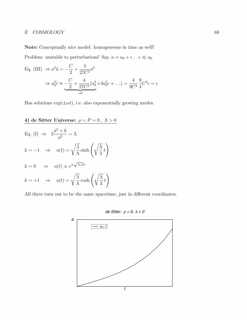
E COSMOLOGY 68
Note: Conceptually nice model: homogeneous in time as well!
Problem: unstable to perturbations! Say, a = a0 + ε , ε a0
Eq. (III) ⇒ a2a = −C2
+4
27C2a3
⇒ a20ε ≈ −
C
2+
4
27C2(a3
0︸ ︷︷ ︸=0
+3a20ε+ . . .) =
4
9C2
9
4C2ε = ε
Has solutions exp(±αt), i.e. also exponentially growing modes.
4) de Sitter Universe: ρ = P = 0 , Λ > 0
Eq. (I) ⇒ 3a2 + k
a2= Λ
k = −1 ⇒ a(t) =
√3
Λsinh
(√Λ
3t
)
k = 0 ⇒ a(t) ∝ e±√
Λ/3 t
k = +1 ⇒ a(t) =
√3
Λcosh
(√Λ
3t
)All three turn out to be the same spacetime, just in different coordinates.
t
a
k=-1
de Sitter: ρ = 0, Λ > 0

E COSMOLOGY 69
5) Λ = 0, radiation dominated: P = ρ/3
From Sec. E.2: in generald
dt(a3ρ) + P
d
dta3 = 0
P = ρ/3 ⇒ 0 =d
dt(a3ρ) + ρa2da
dt= . . . =
1
a
d
dt(a4ρ)
⇒ B ..=8π
3a4ρ = const
We find k = 0 ⇒ a =√
2B1/4√t
k = +1 ⇒ a =√B
√1−
(1− t√
B
)2
k = −1 ⇒ a =√B
√(1 +
t√B
)2
− 1
t
a
k = -1k = 0k = +1
P = ρ/3, Λ = 0
Summary: • Radiation dominated: ρa4 = const
Matter dominated: ρa3 = const
Dark energy: ρ ∝ Λ = const
• Radiation dominant in early universe, dark energy in lateexpanding universe.
• Presently: ∼ 75 % dark energy, 4 % visible matter, ∼ 21 %dark matter, radiation negligible
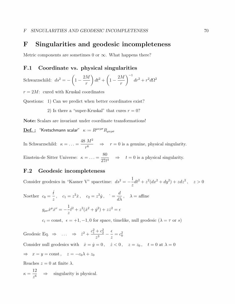
F SINGULARITIES AND GEODESIC INCOMPLETENESS 70
F Singularities and geodesic incompleteness
Metric components are sometimes 0 or ∞. What happens there?
F.1 Coordinate vs. physical singularities
Schwarzschild: ds2 = −(
1− 2M
r
)dt2 +
(1− 2M
r
)−1
dr2 + r2dΩ2
r = 2M : cured with Kruskal coordinates
Questions: 1) Can we predict when better coordinates exist?
2) Is there a “super-Kruskal” that cures r = 0?
Note: Scalars are invariant under coordinate transformations!
Def. : “Kretschmann scalar” κ ..= RµνρσRµνρσ
In Schwarzschild: κ = . . . =48 M2
r6⇒ r = 0 is a genuine, physical singularity.
Einstein-de Sitter Universe: κ = . . . =80
27t4⇒ t = 0 is a physical singularity.
F.2 Geodesic incompleteness
Consider geodesics in “Kasner V” spacetime: ds2 = −1
zdt2 + z2(dx2 + dy2) + zdz2 , z > 0
Noether c0 =t
z, c1 = z2x , c2 = z2y , ˙ =
d
dλ, λ = affine
gµν xµxν = −1
zt2 + z2(x2 + y2) + zz2 = ε
ci = const, ε = +1,−1, 0 for space, timelike, null geodesic (λ = τ or s)
Geodesic Eq. ⇒ . . . ⇒ z2 +c2
1 + c22
z3− ε
z= c2
0
Consider null geodesics with x = y = 0 , z < 0 , z = z0 , t = 0 at λ = 0
⇒ x = y = const , z = −c0λ+ z0
Reaches z = 0 at finite λ.
κ =12
z6⇒ singularity is physical.

F SINGULARITIES AND GEODESIC INCOMPLETENESS 71
Def.: A geodesic is incomplete if it cannot be extended to arbitrarily large values of its parameter,either to the future or the past. The termination point is a singularity.
Can this happen too at coordinate singularities? Yes! Example:
Rindler spacetime: ds2 = −z2dt2 + dx2 + dy2 + dz2 , t, x, y, z, ∈ R , z > 0
Noether: c0 = z2t , c1 = x , c2 = y all const.
−z2t2 + x2 + y2 + z2 = ε = +1, −1 or 0 as in Kasner V
Consider timelike geodesics with x = y = 0 , z < 0 , z = z0 , t = 0 at τ = 0
⇒ . . . ⇒ z(τ) =√z2
0 − τ 2 , t(τ) = artanhτ
z0
geodesic hits singular z = 0 at finite τ
Now transform coordinates: x = X , y = Y , z =√Z2 − T 2 , t = artanh
T
Z
⇒ . . . ⇒ ds2 = −dT 2 + dX2 + dY 2 + dZ2
Rindler spacetime is just a wedge of Minkowski spacetime!
Here the singular point z = 0 can be cured with better coordinates.
Is there a systematic way to find such better coordinates?
In 4 dimensions no, but in 2 dimensions (e.g. spherical symm.) there is: Sec. 6.4 in Wald.

G LINEARIZED THEORY AND GRAVITATIONAL WAVES 72
G Linearized theory and gravitational waves
G.1 Plane waves and pp metrics
Plane waves are common in physics. E.g. electromagnetic waves ~E, ~B ∝ ei(~k~x−ωt)
Rotate coordinates such that ~k = (0, 0, k) ⇒ ~E, ~B ∝ ei(kz−ωt) = eik(z−vt)
phase velocity: v =ω
k
The components satisfy the wave equation 2f = −∂2t f + ~∇2f = 0
With f ∝ ei(~k~x−ωt) ⇒ ω2 − ~k2 = 0 ⇒ k = |~k| = ±ω ⇒ v =
ω
k= ±1 = ±c
SR notation: f ∝ eikαxα
with kα = (−ω, ~k)
2f = ηαβ∂α∂βf = 0 ⇒ kαkα = 0
plane wave in +z direction: kα = (−ω, 0, 0, k)
Plane waves also exist in full GR!
Def.: Spacetimes admitting a covariantly constant vector field V are called pp wave spacetimes.They admit plane wave solutions.
Example: Brinkmann metrics: ds2 = H(u, x, y)du2 + 2du dv + dx2 + dy2
V ..= ∂v satisfies V β = ∂αVβ + ΓβµαV
µ = 0 + Γβµαδµv = Γβvα = . . . = 0
Furthermore: Ruu = 0 ⇒ . . . ⇒ ∂2xH + ∂2
yH = 0
Clearly solved by H = H0 eikαxα , H0 = const , kα = (−ω, 0, 0, ω)
pp metrics are important in the construction of analytic solutions in GR.
E.g. Aichelburg-Sexl metric: Schwarzschild BH boosted to the speed of light.
G.2 Linearized theory
Consider a system close to a known solution: Metric = background + perturbation
For us background is Minkowski, but idea works for general backgrounds: perturbation theory
⇒ gµν = ηµν + hµν , ηµν = diag(−1, 1, 1, 1) , hµν = O(ε) 1
We regard hµν as a tensor field on Minkowski background

G LINEARIZED THEORY AND GRAVITATIONAL WAVES 73
inverse metric: gµν = ηµν + kµν
⇒ gµνgνρ = δµρ + kµνηνρ + ηµνhνρ + kµνhνρ︸ ︷︷ ︸=O(ε2)→0
!= δµρ
⇒ kµν = −ηµρηνσhρσ =: −hµν = O(ε)
To O(ε): Γµνρ =1
2ηµσ(∂ρhσν + ∂νhρσ − ∂σhνρ) ,
Rµνρσ = ηµτ(∂ρΓ
τνσ − ∂σΓτνρ
) ∣∣∣ Γ · Γ = O(ε2)
= 12
(∂ρ∂νhµσ + ∂σ∂µhνρ − ∂ρ∂µhνσ − ∂σ∂νhµρ
)Rµν = ∂ρ∂(µhν)ρ −
1
2∂ρ∂ρhµν −
1
2∂µ∂νh
∣∣∣ h := hµµ , ∂µ := gµρ∂ρ
Gµν = ∂ρ∂(µhν)ρ −1
2∂ρ∂ρhµν −
1
2∂µ∂νh−
1
2ηµν(∂
ρ∂σhρσ − ∂ρ∂ρh)!
= 8πTµν
⇒ Tµν 1
Def.: “trace-reversed perturbation” hµν ..= hµν −1
2hηµν ⇔ hµν = hµν −
1
2hηµν ,
h = hµµ = −h
⇒ . . .⇒ Gµν = −1
2∂ρ∂ρhµν + ∂ρ∂(µhν)ρ −
1
2ηµν∂
ρ∂σhρσ = 8πTµν
Coordinate freedom
xα = xα − ξα , ξα = O(ε) ⇒ ∂xα
∂xµ= δαµ − ∂µξα ,
∂xν
∂xβ= δνβ + ∂βξ
ν
⇒ gµν = ηµν + hµν , hµν = hµν + ∂µξν + ∂νξµ +O(ε2)
Note: • Background unchanged
• 4 free functions: We choose ξµ such that ∂ν∂νξµ = −∂ν hµν
⇒ . . . ⇒ ∂ν ¯hµν = 0 “Lorentz gauge”
⇒ − 2Gµν = 2¯hµµ = ∂ρ∂ρ¯hµν = −16πTµν
Wave equation! drop ˜ from now on.

G LINEARIZED THEORY AND GRAVITATIONAL WAVES 74
G.3 The Newtonian limit
Newtonian gravity: ~∇2Φ = 4πρ ; Φ ∼ v2 1 (Sec. A.1) , ε ..=v2
c2= v2
⇒ matter sources weak: ρ ∼ O(ε)
Newtonian matter: T00 = ρ+O(ε2)
T0i ∼ T00 vi ∼ O(ε3/2)
Tij ∼ T00 vivj ∼ O(ε2)
E.g. perfect fluid: Tµν = (ρ+ P )uµuν + Pgµν , P ∼ ρv2 ≈ 10−5 ρ in sun
In Newt. gravity temporal changes in Φ are caused by motion of sources
⇒ ∂
∂t∼ v
∂
∂xi= O(ε1/2)
∂
∂xi
⇒ 2hµν = ∂ρ∂ρhµν = ∂i∂ihµν = ~∇2hµν = −16πTµν
⇒ ~∇2h00 = −16πT00 = −16πρ+O(ε2) , h0i = O(ε3/2) , hij = O(ε2)
Newton’s law with h00 = −4Φ
⇒ h = ηµν hµν = 4Φ +O(ε2) = −h
⇒ h00 = h00 −1
2η00h = −2Φ , hij = hij −
1
2ηijh = −2Φδij
or ds2 = −(1 + 2Φ)dt2 + (1− 2Φ)(dx2 + dy2 + dz2) cf. Sec. A.2
Geodesics
L = (1+2Φ)t2−δij(1−2Φ)xixj!
= 1 ⇒ t2 = (1+2Φ)−1[1+δijx
ixj+O(ε2)]
⇒ t = 1− Φ +1
2δijx
ixj +O(ε2)
EL for xk:d
dτ
L∂xk
=d
dτ
[− 2δjk(1− 2Φ)xj
]=
∂L∂xk
= 2∂kΦ (t2 + δijxixj)︸ ︷︷ ︸
=1+O(ε)
⇒ xk =d2xkdτ 2
=d2xkdt2
= −∂kΦ to O(ε) ; test body in Newt. gravity
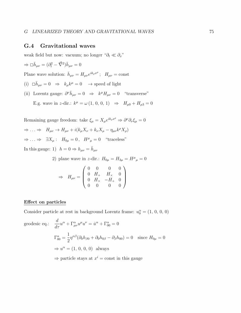
G LINEARIZED THEORY AND GRAVITATIONAL WAVES 75
G.4 Gravitational waves
weak field but now: vacuum; no longer “∂t ∂x”
⇒ 2hµν = (∂2t − ~∇2)hµν = 0
Plane wave solution: hµν = Hµνeikρxρ ; Hµν = const
(i) 2hµν = 0 ⇒ kµkµ = 0 → speed of light
(ii) Lorentz gauge: ∂ν hµν = 0 ⇒ kµHµν = 0 “transverse”
E.g. wave in z-dir.: kµ = ω (1, 0, 0, 1) ⇒ Hµ0 +Hµ3 = 0
Remaining gauge freedom: take ξµ = Xµeikρxρ ⇒ ∂ν∂νξµ = 0
⇒ . . .⇒ Hµν → Hµν + i(kµXν + kνXµ − ηµνkρXρ)
⇒ . . .⇒ ∃Xµ : H0µ = 0 , Hµµ = 0 “traceless”
In this gauge: 1) h = 0⇒ hµν = hµν
2) plane wave in z-dir.: H0µ = H3µ = Hµµ = 0
⇒ Hµν =
0 0 0 00 H+ H× 00 H× −H+ 00 0 0 0
Effect on particles
Consider particle at rest in background Lorentz frame: uα0 = (1, 0, 0, 0)
geodesic eq.:d
dτuα + Γαµνu
µuν = uα + Γα00 = 0
Γα00 =1
2ηαβ(∂0hβ0 + ∂0h0β − ∂βh00) = 0 since H0µ = 0
⇒ uα = (1, 0, 0, 0) always
⇒ particle stays at xi = const in this gauge
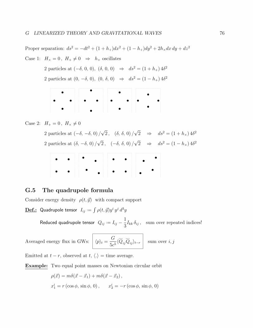
G LINEARIZED THEORY AND GRAVITATIONAL WAVES 76
Proper separation: ds2 = −dt2 + (1 + h+)dx2 + (1− h+)dy2 + 2h×dx dy + dz2
Case 1: H× = 0 , H+ 6= 0 ⇒ h+ oscillates
2 particles at (−δ, 0, 0), (δ, 0, 0) ⇒ ds2 = (1 + h+) 4δ2
2 particles at (0, −δ, 0), (0, δ, 0) ⇒ ds2 = (1− h+) 4δ2
Case 2: H+ = 0 , H× 6= 0
2 particles at (−δ, −δ, 0) /√
2 , (δ, δ, 0) /√
2 ⇒ ds2 = (1 + h×) 4δ2
2 particles at (δ, −δ, 0) /√
2 , (−δ, δ, 0) /√
2 ⇒ ds2 = (1− h×) 4δ2
G.5 The quadrupole formula
Consider energy density ρ(t, ~y) with compact support
Def.: Quadrupole tensor Iij ..=∫ρ(t, ~y)yi yj d3y
Reduced quadrupole tensor Qij..= Iij −
1
3Ikk δij , sum over repeated indices!
Averaged energy flux in GWs: 〈p〉t =G
5c5〈...Qij
...Qij〉t−r sum over i, j
Emitted at t− r, observed at t, 〈.〉 = time average.
Example: Two equal point masses on Newtonian circular orbit
ρ(~x) = mδ(~x− ~x1) +mδ(~x− ~x2) ,
xi1 = r (cosφ, sinφ, 0) , xi2 = −r (cosφ, sinφ, 0)

G LINEARIZED THEORY AND GRAVITATIONAL WAVES 77
Newtonian orbit: ω = φ =
√Gm
4r3
⇒ Ixx = 2mr2 cos2 ωt = mr2(1 + cos 2ωt)
Iyy = 2mr2 sin2 ωt = 2mr2(1− cos2 ωt) = mr2(1− cos 2ωt)
Ixy = Iyx = 2mr2 cosωt sinωt = mr2 sin 2ωt
Qij = Iij −2
3mr2 = Iij − const
⇒...Qxx = 8ω3mr2 sin 2ωt...Qyy = −8ω3mr2 sin 2ωt
...Qxy =
...Qyx = −8ω3mr2 cos 2ωt
Adding all up: 〈p〉t =2
5
G4
c5
m5
r5
Gravitational waves directly detected on 14 Sep 2015: New window to the universe!

REFERENCES 78
References
[1] S. M. Carroll. Lecture notes on general relativity, 1997. gr-qc/9712019.
[2] S. M. Carroll. Spacetime and Geometry: An Introduction to General Relativity. Pearson,2003.
[3] R. d’Inverno. Introducing Einstein’s Relativity. Oxford: Clarendon Press, 1992. ISBN-9780198596868.
[4] J. B. Hartle. Gravity: An Introduction to Einstein’s General Relativity. Pearson, 2014.
[5] L. Ryder. Introduction to General Relativity. Cambridge University Press, 2009.
[6] B. F. Schutz. A First Course in General Relativity. Cambridge University Press, 2009. 2ndEdition.