part ii chapter 6 applications of...
TRANSCRIPT
C H A P T E R 6Applications of Integration
Section 6.1 Area of a Region Between Two Curves . . . . . . . . . . 264
Section 6.2 Volume: The Disk Method . . . . . . . . . . . . . . . . . 271
Section 6.3 Volume: The Shell Method . . . . . . . . . . . . . . . . 278
Section 6.4 Arc Length and Surfaces of Revolution . . . . . . . . . . 282
Section 6.5 Work . . . . . . . . . . . . . . . . . . . . . . . . . . . . 287
Section 6.6 Moments, Centers of Mass, and Centroids . . . . . . . . . 290
Section 6.7 Fluid Pressure and Fluid Force . . . . . . . . . . . . . . . 297
Review Exercises . . . . . . . . . . . . . . . . . . . . . . . . . . . . . 299
Problem Solving . . . . . . . . . . . . . . . . . . . . . . . . . . . . . . 305
P A R T I I

C H A P T E R 6Applications of Integration
Section 6.1 Area of a Region Between Two CurvesSolutions to Even-Numbered Exercises
264
2. A � �2
�2 ��2x � 5� � �x2 � 2x � 1�� dx � �2
�2 ��x2 � 4� dx
4. A � �1
0 �x2 � x3� dx 6. A � 2�1
0 ��x � 1�3 � �x � 1�� dx
8.
x−2 2
−2
2
y
�1
�1 ��1 � x2� � �x2 � 1�� dx 10.
1
−1
2
2 4 5 6 7
3
4
5
6
7(3, 6)
(3, 1)
23
2,( )
y
x
�3
2��x3
3� x �
x
3 dx 12.
π4
π4−
π4− 2
2,( )
π4− , 2( ) π
4 , 2( )
π4
22,( )
y
x
2
3
���4
���4�sec2 x � cos x� dx
14.
Matches (a)
x
1
3
4
1 2 3
(0, 2)
(4, 0)
y
A � 1
g�x� � 2 � x
f �x� � 2 �12 x 16.
2
2
4
6
8
4 6 10
y
x
(2, 9)
2,
(8, 6)
(8, 0)
92( )
� �64 � 112 � 80� � �1 � 7 � 20� � 18
� �x3
8�
7x2
4� 10x
8
2
� �8
2�3
8x2 �
72
x � 10 dx
A � �8
2��10 �
12
x � ��38
x�x � 8� dx
Section 6.1 Area of a Region Between Two Curves 265
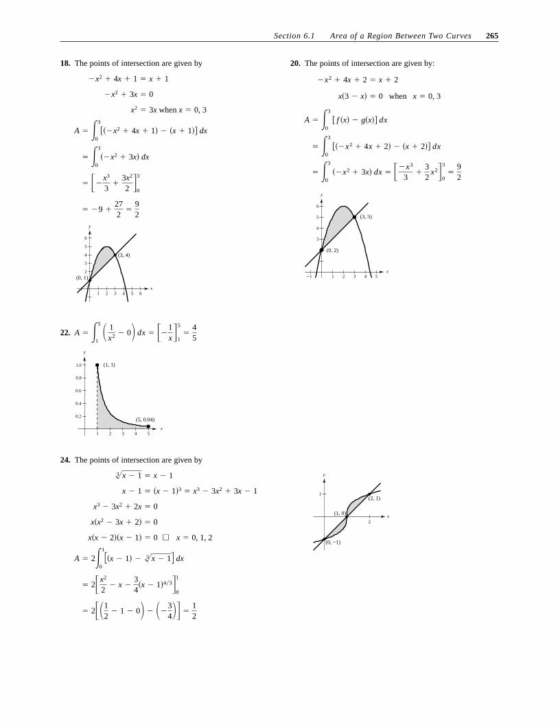
18. The points of intersection are given by
(3, 4)
(0, 1)
1 2
2
3
4
5
6
3 4 5 6
y
x
� �9 �272
�92
� ��x3
3�
3x2
2 3
0
� �3
0��x2 � 3x� dx
A � �3
0���x2 � 4x � 1� � �x � 1�� dx
x2 � 3x when x � 0, 3
�x2 � 3x � 0
�x2 � 4x � 1 � x � 1
20. The points of intersection are given by:
x−1 1 2 3 4 5
3
4
5
6
(0, 2)
(3, 5)
y
� �3
0 ��x2 � 3x� dx � ��x3
3�
32
x23
0�
92
� �3
0 ���x2 � 4x � 2� � �x � 2�� dx
A � �3
0 � f �x� � g�x�� dx
x�3 � x� � 0 when x � 0, 3
�x2 � 4x � 2 � x � 2
22.
x1 2 3 4 5
0.2
0.4
0.6
0.8
1.0 (1, 1)
(5, 0.04)
y
A � �5
1 � 1
x2 � 0 dx � ��1x
5
1�
45
24. The points of intersection are given by
� 2��12
� 1 � 0 � ��34 �
12
� 2�x2
2� x �
34
�x � 1�4�31
0
A � 2�1
0��x � 1� � 3 x � 1� dx
x�x � 2��x � 1� � 0 ⇒ x � 0, 1, 2
x�x2 � 3x � 2� � 0
x3 � 3x2 � 2x � 0
x � 1 � �x � 1�3 � x3 � 3x2 � 3x � 1 1
2
(0, −1)
(1, 0)
(2, 1)
y
x
3 x � 1 � x � 1

266 Chapter 6 Applications of Integration
26. The points of intersection are given by:
� �3
0 �3y � y2� dy � �3
2y2 �
13
y33
0�
92
� �3
0 ��2y � y2� � ��y�� dy
A � �3
0 � f �y� � g�y�� dy
y�y � 3� � 0 when y � 0, 3
x
−1
1
3
−3 −2 1
( 3, 3)−
(0, 0)
y 2y � y2 � �y
28.
� �� 16 � y23
0� 4 � 7 � 1.354
� �12
�3
0 �16 � y2��1�2��2y� dy
� �3
0 � y 16 � y2
� 0 dy
x
1
2
3
4
−1 1 2 3
( ), 37
3
y
A � �3
0 � f �y� � g�y�� dy
30.
� 1.227
� 4 � 4 ln 2
� �4x � 4 ln �2 � x�1
0
x
1
3
−1 1 3
(0, 2)
(1, 4)
y
A � �1
0 �4 �
42 � x dx
32. The point of intersection is given by:
Numerical Approximation: 2.0
x−2 −1 2
−2
−1
( 1, 2)−
(1, 0)
(1, 2)−
y
� �1
�1 �x3 � 1� dx � �x4
4� x
1
�1� 2
� �1
�1 ��x3 � 2x � 1� � ��2x�� dx
A � �1
�1 � f �x� � g�x�� dx
x3 � 1 � 0 when x � �1
x3 � 2x � 1 � �2x
34. The points of intersection are given by:
Numerical Approximation: 8.533
( 2, 8)−
(0, 0)
(2, 8)
−4 4
−2
10
� 2 �4x3
3�
x5
5 2
0�
12815
� 2 �2
0 �4x2 � x4� dx
A � 2 �2
0 �2x2 � �x4 � 2x2�� dx
x2�x2 � 4� � 0 when x � 0, ±2
x4 � 2x2 � 2x2
Section 6.1 Area of a Region Between Two Curves 267
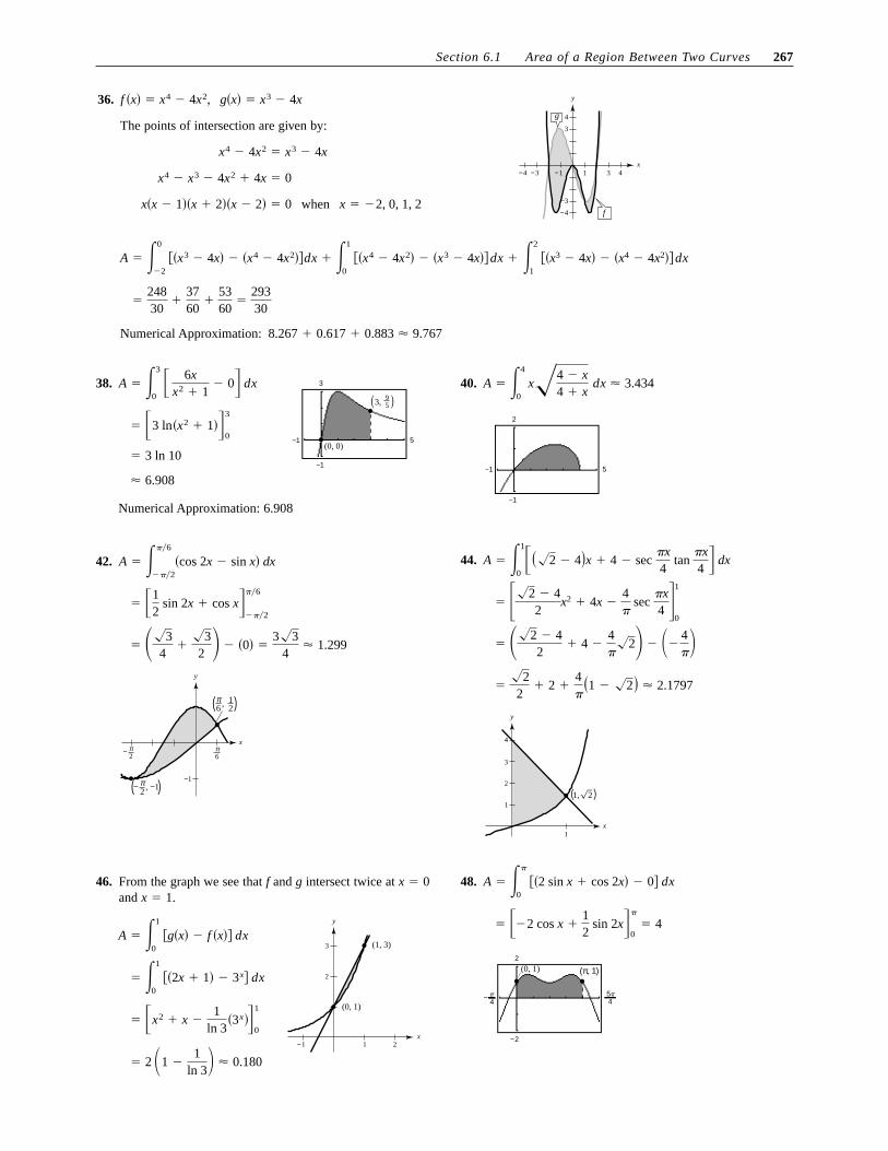
36.
The points of intersection are given by:
Numerical Approximation: 8.267 � 0.617 � 0.883 � 9.767
�29330
�24830
�3760
�5360
�2
1 ��x3 � 4x� � �x4 � 4x2�� dx A � �0
�2 ��x3 � 4x� � �x4 � 4x2�� dx � �1
0 ��x4 � 4x2� � �x3 � 4x�� dx �
x�x � 1��x � 2��x � 2� � 0 when x � �2, 0, 1, 2
x4 � x3 � 4x2 � 4x � 0
x4 � 4x2 � x3 � 4xx
−1−3−4 1 3 4
−3
−4
3
4
f
g
yf �x� � x4 � 4x2, g�x� � x3 � 4x
38.
Numerical Approximation: 6.908
� 6.908
� 3 ln 10
� �3 ln�x2 � 1�3
0(0, 0)
3, 95( )
−1 5
−1
3 A � �3
0 � 6x
x2 � 1� 0 dx 40.
−1 5
−1
2
A � �4
0 x 4 � x
4 � x dx � 3.434
42.
π2
π6
−
π2
−
−1, −1( )
π6 2
1, ( )
y
x
� � 34
� 32 � �0� �
3 34
� 1.299
� �12
sin 2x � cos x��6
���2
A � ���6
���2�cos 2x � sin x� dx 44.
1, 2 )(
1
1
2
3
4
y
x
� 22
� 2 �4�
�1 � 2� � 2.1797
� � 2 � 42
� 4 �4� 2 � ��
4�
� � 2 � 42
x2 � 4x �4�
sec �x4
1
0
A � �1
0�� 2 � 4�x � 4 � sec
�x4
tan �x4 dx
46. From the graph we see that f and g intersect twice at and
� 2 �1 �1
ln 3 � 0.180
� �x2 � x �1
ln 3�3x�
1
0
� �1
0 ��2x � 1� � 3x� dx
A � �1
0 �g�x� � f �x�� dx
x � 1.x � 0
x
2
3
−1 1 2
(0, 1)
(1, 3)
y
48.
−2
(0, 1)
−
(π, 1)2
�4
�45
� ��2 cos x �12
sin 2x�
0� 4
A � ��
0 ��2 sin x � cos 2x� � 0� dx
268 Chapter 6 Applications of Integration
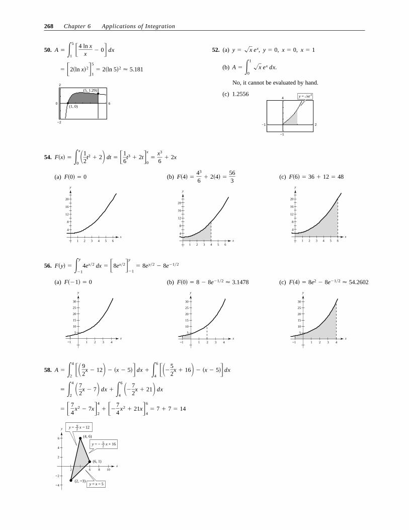
50.
(1, 0)
(5, 1.29)
−2
0 6
2
� 5.181� 2�ln 5�2 � �2�ln x�25
1
A � �5
1 �4 ln x
x� 0 dx 52. (a)
(b)
No, it cannot be evaluated by hand.
(c) 1.2556
−1
−1
2
4 y xe= x
A � �1
0 x ex dx.
x � 1x � 0,y � 0,y � x ex,
54. F�x� � �x
0�1
2t2 � 2 dt � �1
6t3 � 2t
x
0�
x3
6� 2x
(a)
1 2 3 4
4
8
12
16
20
5 6
y
x
F�0� � 0 (b)
1 2 3 4
4
8
12
16
20
5 6
y
x
F�4� �43
6� 2�4� �
563
(c)
1 2 3 4
4
8
12
16
20
5 6
y
x
F�6� � 36 � 12 � 48
56. F�y� � �y
�14ex�2 dx � �8ex�2
y
�1� 8ey�2 � 8e�1�2
(a)
10
5
15
20
25
30
−1 1 2 3 4
y
x
F��1� � 0 (b)
10
5
15
20
25
30
−1 1 2 3 4
y
x
F�0� � 8 � 8e�1�2 � 3.1478 (c)
10
5
15
20
25
30
−1 1 2 3 4
y
x
F�4� � 8e2 � 8e�1�2 � 54.2602
58.
(4, 6)
(6, 1)
(2, 3)−y x= 5−
52y x= + 16−
92y x= 12−y
x2 6 8 10
−4
−2
2
4
6
� � 74
x2 � 7x4
2� ��7
4x2 � 21x
6
4� 7 � 7 � 14
� �4
2 � 7
2x � 7 dx � �6
4 ��7
2x � 21 dx
A � �4
2 �� 9
2x � 12 � �x � 5� dx � �6
4 ���5
2x � 16 � �x � 5� dx

Section 6.1 Area of a Region Between Two Curves 269
60.
At .
Tangent line:
or
The tangent line intersects at
A � �1
0 � 1
x2 � 1� ��1
2 x � 1 dx � �arctan x �
x2
4� x
1
0�
� � 34
� 0.0354
x � 0.f �x� �1
x2 � 1
y � �12
x � 1y �12
� �12
�x � 1�
f��1� � �12�1,
12,
f��x� � �2x
�x2 � 1�2
f �x� �1
x2 � 1
x1 2
(0, 1)
1,
12
12
14
32
34
( )
f x( ) =1
2x + 1
12
12
y x= + 1−
y
64. on
on
Both functions symmetric to origin
Thus,
A � 2 �1
0 �x � x3� dx � 2 �x2
2�
x4
4 1
0�
12
�1
�1 �x3 � x� dx � 0.
�0
�1 �x3 � x� dx � ��1
0 �x3 � x� dx.
�0, 1�x3 ≤ x
��1, 0�x3 ≥ x
x
( 1, 1)− −
(0, 0)
(1, 1)1
1
−1
−1
y
62. Answers will vary. See page 417.
66. Proposal 2 is better, since the cummulative deficit (the area under the curve) is less.
68.
b � 9 �9 2
� 2.636
9 � b �9 2
�9 � b��9 � b� �812
2 ��9 � b�x �x2
2 9�b
0�
812
2�9�b
0 ��9 � b� � x� dx �
812
2 �9�b
0 ��9 � x� � b� dx �
812
A � 2 �9
0 �9 � x� dx � 2 �9x �
x2
2 9
0� 81
x
( (9 ), )− −b b (9 , )−b b
−6 −3 3 6
−3
−6
6
9
12
y
270 Chapter 6 Applications of Integration
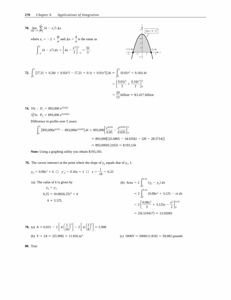
70.
where and is the same as
�2
�2 �4 � x2� dx � �4x �
x3
3 2
�2�
323
.
�x �4n
xi � �2 �4in
lim���→0
�n
i�1 �4 � xi
2� �x
x
5
3
2
1
−1
−3 −1 1 3
( 2, 0)− (2, 0)
f x x( ) = 4 − 2
y
72.
�2912
billion � $2.417 billion
� �0.01t3
3�
0.16t2
2 5
0
�5
0 ��7.21 � 0.26t � 0.02t2� � �7.21 � 0.1t � 0.01t2�� dt � �5
0 �0.01t2 � 0.16t� dt
74. 5% :
Difference in profits over 5 years:
Note: Using a graphing utility you obtain $193,183.
� 893,000�0.2163� � $193,156
� 893,000��25.6805 � 34.0356� � �20 � 28.5714��
�5
0 �893,000e0.05t � 893,000e0.035t� dt � 893,000�e0.05t
0.05�
e0.035t
0.0355
0
P2 � 893,000 e�0.035�t312 %:
P1 � 893,000 e�0.05�t
76. The curves intersect at the point where the slope of equals that of
y2 � 0.08x2 � k ⇒ y�2 � 0.16x � 1 ⇒ x �1
.16� 6.25
y1, 1.y2
(b)
� 2�6.510417� � 13.02083
� 2 �0.08x3
3� 3.125x �
x2
2 6.25
0
� 2 �6.25
0 �0.08x2 � 3.125 � x� dx
Area � 2 �6.25
0 �y2 � y1� dx(a) The value of k is given by
k � 3.125.
6.25 � �0.08��6.25�2 � k
y1 � y2
78. (a)
(b) (c) 5000V � 5000�11.816� � 59,082 poundsV � 2A � 2�5.908� � 11.816 m3
A � 6.031 � 2 �� � 116
2
� 2 �� �18
2
� 5.908
80. True

Section 6.2 Volume: The Disk Method
Section 6.2 Volume: The Disk Method 271
2. V � � �2
0 �4 � x2�2 dx � � �2
0 �x4 � 8x2 � 16� dx � ��x5
5�
8x3
3� 16x�
2
0�
256�
15
4.
� ��9x �x3
3 �3
0� 18�
V � ��3
0��9 � x2�2 dx � ��3
0�9 � x2� dx 6.
x � ±2�2
x2 � 8
8 � 16 � x2
2 � 4 �x2
4
�448�2
15� � 132.69
� 2��128�280
�32�2
3� 24�2�
� 2�� x5
80�
2x3
3� 12x�
2�2
0
� 2��2�2
0� x4
16� 2x2 � 12� dx
V � ��2�2
�2�2�4 �
x2
4 2
� �2�2� dx
8.
� ��16y �y3
3 �4
0�
128�
3
V � � �4
0 ��16 � y2 �2 dy � ��4
0 �16 � y2� dy
y � �16 � x2 ⇒ x � �16 � y2 10.
�459�
15�
153�
5
� ��y5
5� 2y4 �
16y3
3 �4
1
V � ��4
1 ��y2 � 4y�2 dy � ��4
1 �y4 � 8y3 � 16y2� dy
12. x � 2y � 0,y � 2x2,
(b)
x−4 −2 2 4
2
4
6
8
y
V � ��2
0 4x4 dx � � �4x5
5 �2
0�
128�
5
r�x� � 0R�x� � 2x2,(a)
x−4 −2 2 4
2
4
6
8
y
V � ��8
0 4 �
y2 dy � ��4y �
y2
4 �8
0� 16�
r�y� � �y�2R�y� � 2,
(c)
x−4 −2 2 4
2
4
6
y
� 4��83
x3 �15
x5�2
0�
896�
15
� ��2
0 �32x2 � 4x4� dx � 4��2
0 �8x2 � x4� dx
V � ��2
0 �64 � �64 � 32x2 � 4x4� dx
r�x� � 8 � 2x2R�x� � 8, (d)
x−4 −2 4
2
4
6
8
y
� ��4y �4�2
3y3�2 �
y2
4 �8
0
�16�
3
� ��8
04 � 4�y
2�
y2 dy
V � ��8
0 2 ��y
2 2
dy
r�y� � 0R�y� � 2 � �y�2,

272 Chapter 6 Applications of Integration
14. intersect at and �0, 6�.��3, 3�y � x � 6y � 6 � 2x � x2,
(b)
x−6 −4 −2 2
2
4
8
y
� �� 15
x5 � x4 � x3 � 9x2�0
�3�
108�
5
� ��0
�3�x4 � 4x3 � 3x2 � 18x� dx
V � ��0
�3��3 � 2x � x2�2 � �x � 3�2 dx
r�x� � �x � 6� � 3R�x� � �6 � 2x � x2� � 3,(a)
x−6 −4 −2 2
2
4
8
y
� ��15
x5 � x4 � 3x3 � 18x2�0
�3�
243�
5
� ��0
�3�x4 � 4x3 � 9x2 � 36x� dx
V � ��0
�3��6 � 2x � x2�2 � �x � 6�2 dx
r�x� � x � 6R�x� � 6 � 2x � x2,
16.
1
1−1−1
2 3 4
2
3
(2, 4)
y
x
� ��32 � 16 �12828 � �
1447
�
� ��16x � x4 �x7
28�2
0
� ��2
0�16 � 4x3 �
x6
4 � dx
V � ��2
04 �
x3
2 2
dx
R�x� � 4 �x3
2, r�x� � 0 18.
x
1
2
3
5
2π π 4π 5ππ9 9 3 9 9
y
� ��8 ln�2 � �3 � � �3 � 27.66
� ���8 ln�2 � �3 � � �3 � � �8 ln�1 � 0� � 0�
� ��8 ln�sec x � tan x� � tan x���3
0
� ����3
0�8 sec x � sec2 x� dx
V � ����3
0��4�2 � �4 � sec x�2 dx
r�x� � 4 � sec xR�x� � 4,
20.
� ��36y �y3
3 �4
0�
368�
3
V � ��4
0��6�2 � �y�2 dy
r�y� � 6 � �6 � y� � yR�y� � 6,
x1 2 3 4 5
1
−1
2
3
4
5
y
Section 6.2 Volume: The Disk Method 273
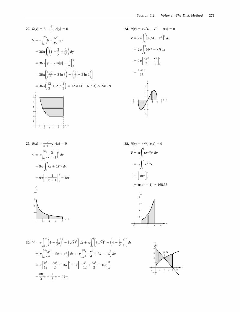
22.
x
1
2
3
4
5
6
1 2 3 4 5
y
� 12��13 � 6 ln 3� � 241.59 � 36� 133
� 2 ln 13
� 36��356
� 2 ln 6 � 32
� 2 ln 2�
� 36��y � 2 ln�y� �1y �
6
2
� 36��6
21 �
2y
�1y2 dy
V � ��6
26 �
6y
2
dy
r�y� � 0R�y� � 6 �6y
, 24.
x
−3
−2
1
2
3
−3 −1 1 2 3
y
�128�
15
� 2��4x3
3�
x5
5 �2
0
� 2��2
0�4x2 � x4� dx
V � 2��2
0�x�4 � x2 2
dx
r�x� � 0R�x� � x�4 � x2,
26.
x2 4 6 8
1
2
3
4
y
� 9��� 1x � 1�
8
0� 8�
� 9� �8
0�x � 1��2 dx
V � ��8
0 3
x � 12
dx
r�x� � 0R�x� �3
x � 1, 28.
x−2 2 4 6
2
4
6
8
y
� ��e4 � 1� � 168.38
� ��ex�4
0
� ��4
0 ex dx
V � ��4
0�ex�2�2 dx
r�x� � 0R�x� � e x�2,
30.
�883
� �563
� � 48�
� �� x3
12�
5x2
2� 16x�
4
0� ���
x3
12�
5x2
2� 16x�
8
4
� ��4
0x2
4� 5x � 16 dx � ��8
4�
x2
4� 5x � 16 dx
2−2−1
1
2
3
4
4 6 8 10
(4, 2)
y
x
V � ��4
0�4 �
12
x2
� ��x�2� dx � ��8
4���x�2
� 4 �12
x2
� dx
274 Chapter 6 Applications of Integration
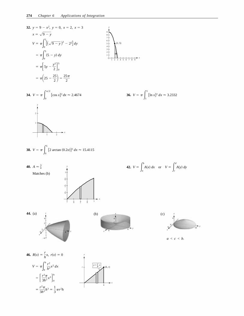
32.
� �25 �252 �
25�
2
� ��5y �y2
2 �5
0
� ��5
0�5 � y� dy
V � ��5
0���9 � y �2
� 22 dy
x � �9 � y
(2, 5)
1 2 3 4 5 6 7 8 9
1
2
3
4
5
6
7
8
9
x
yx � 3x � 2,y � 0,y � 9 � x2,
34.
x1 2
1
2
y
V � � ���2
0 �cos x 2 dx � 2.4674 36. V � � �3
1 �ln x 2 dx � 3.2332
38. V � � �5
0 �2 arctan �0.2x� 2 dx � 15.4115
40.
Matches (b)
x
1
134
34
12
12
14
14
yA � 34 42. or V � �d
c
A�y� dyV � �b
a
A�x� dx
44. (a)
x
y842
4
−4
2
z (b)
x
y88
4
2
z (c)
a < c < b.
x
y168
4
4
z
46.
�r2�
3h2 h3 �13
�r2h
� � r2�
3h2 x3�h
0
V � ��h
0 r2
h2 x2 dx
xh
r ( , )h ry = r
hx
yr�x� � 0R�x� �rh
x,
Section 6.2 Volume: The Disk Method 275
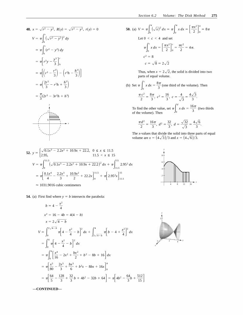
48.
x
r
h
y
��
3�2r3 � 3r2h � h3�
� � 2r3
3� r2h �
h3
3
� ��r3 �r3
3 � r2h �h3
3 �
� ��r2y �y3
3 �r
h
� ��r
h
�r2 � y2� dy
V � ��r
h��r2 � y2 �2 dy
r�y� � 0R�y� � �r2 � y2,x � �r2 � y2, 50. (a)
Let and set
Thus, when the solid is divided into twoparts of equal volume.
x � 2�2,
c � �8 � 2�2
c2 � 8
��c
0 x dx � ��x2
2 �c
0�
�c2
2� 4�.
0 < c < 4
V � ��4
0��x �2 dx � ��4
0 x dx � ��x2
2 �4
0� 8�
(b) Set (one third of the volume). Then
To find the other value, set (two thirdsof the volume). Then
The x-values that divide the solid into three parts of equalvolume are and x � �4�6 ��3.x � �4�3 ��3
d ��32�3
�4�6
3.d 2 �
323
,� d 2
2�
16�
3,
��d
0 x dx �
16�
3
c �4�3
�4�3
3.c2 �
163
,� c2
2�
8�
3,
� �c
0 x dx �
8�
3
52.
� 1031.9016 cubic centimeters
� ��0.1x4
4�
2.2x3
3�
10.9x2
2� 22.2x�
11.5
0� ��2.952x�
15
11.5
V � ��11.5
0��0.1x3 � 2.2x2 � 10.9x � 22.2 �2 dx � ��15
11.5 2.952 dx
y � ��0.1x3 � 2.2x2 � 10.9x � 22.2,2.95,
0 ≤ x ≤ 11.5 11.5 < x ≤ 15
x
2
4
6
8
4 8 12 16
y
x
y
5
42 2
z
54. (a) First find where intersects the parabola:
—CONTINUED—
� ��4b2 �643
b �51215 � � ��64
5�
1283
�323
b � 4b2 � 32b � 64�
� �� x5
80�
2x3
3�
bx3
6� b2x � 8bx � 16x�
4
0
� ��4
0� x4
16� 2x2 �
bx 2
2� b 2 � 8b � 16� dx
� �4
0 ��4 �
x2
4� b�
2
dx
V � �2�4�b
0 ��4 �
x2
4� b�
2
dx � �4
2�4�b
��b � 4 �x2
4 �2
dx
x � 2�4 � b
x2 � 16 � 4b � 4�4 � b�
b � 4 �x2
4
y � b
276 Chapter 6 Applications of Integration
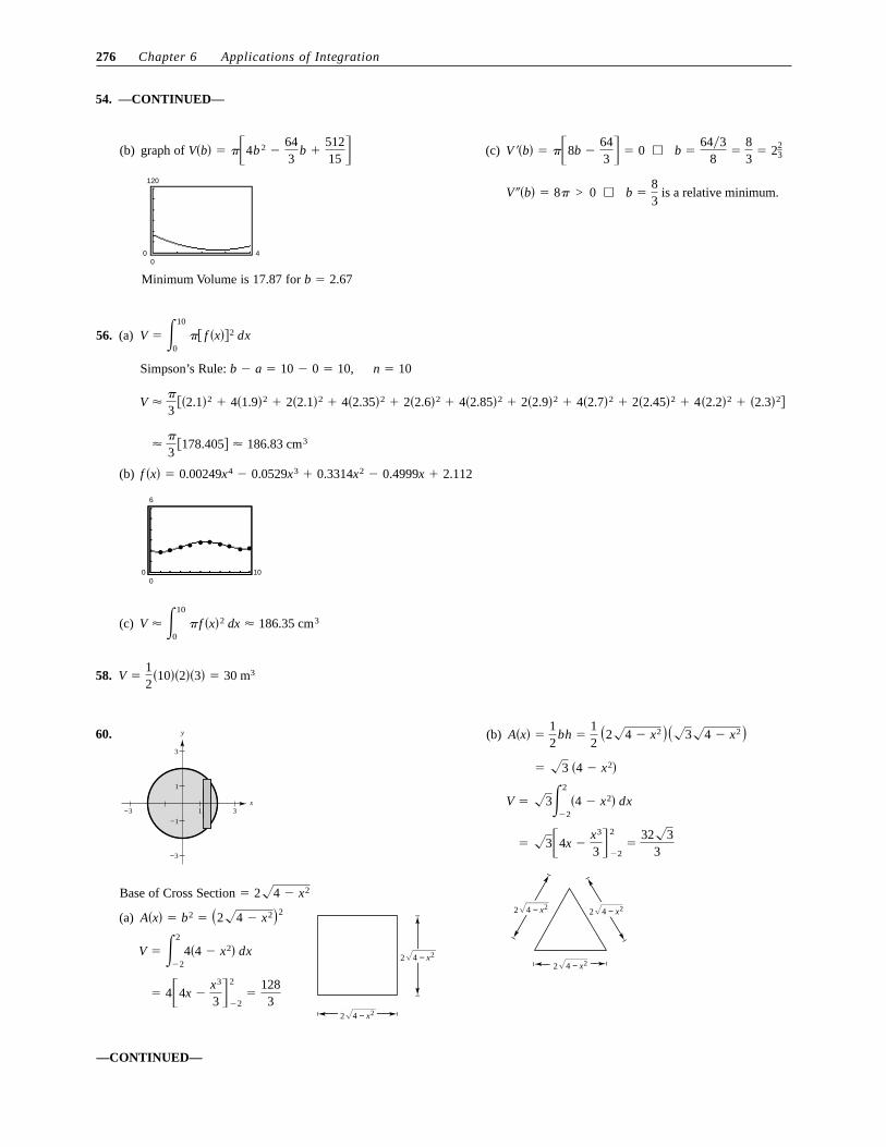
(b) graph of
Minimum Volume is 17.87 for b � 2.67
00
4
120
V�b� � ��4b 2 �643
b �51215 � (c)
V� �b� � 8� > 0 ⇒ b �83
is a relative minimum.
V��b� � ��8b �643 � � 0 ⇒ b �
64�38
�83
� 223
56. (a)
Simpson’s Rule:
��
3�178.405 � 186.83 cm3
� 2�2.9�2 � 4�2.7�2 � 2�2.45�2 � 4�2.2�2 � �2.3�2 V ��
3��2.1�2 � 4�1.9�2 � 2�2.1�2 � 4�2.35�2 � 2�2.6�2 � 4�2.85�2
n � 10b � a � 10 � 0 � 10,
V � �10
0 �� f �x� 2 dx
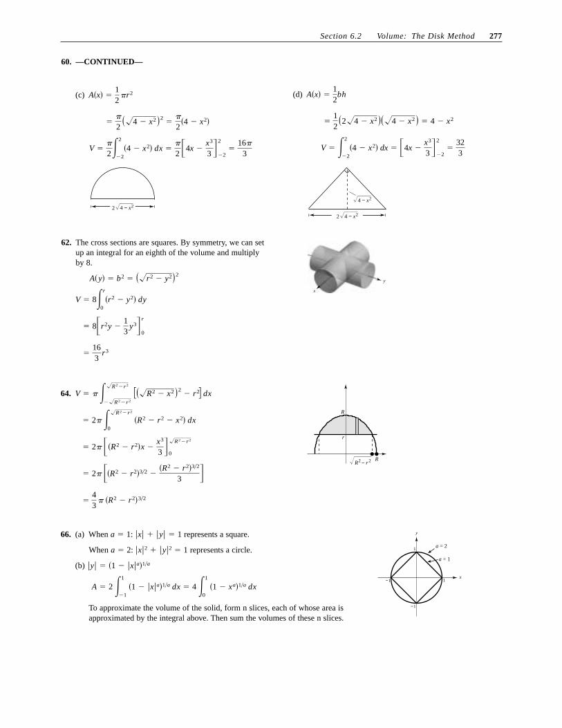
(b)
00
10
6
f �x� � 0.00249x4 � 0.0529x3 � 0.3314x2 � 0.4999x � 2.112
(c) V � �10
0 � f �x�2 dx � 186.35 cm3
58. V �12
�10��2��3� � 30 m3
54. —CONTINUED—
—CONTINUED—
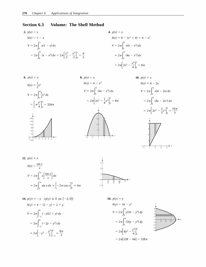
60.
Base of Cross Section
(a)
� 4�4x �x3
3 �2
�2�
1283
V � �2
�24�4 � x2� dx
2 4 − x2
2 4 − x2
A�x� � b2 � �2�4 � x2�2
� 2�4 � x2
x
3
1
1
−1
−3
3−3
y (b)
2 4 − x22 4 − x2
2 4 − x2
� �3�4x �x3
3 �2
�2�
32�33
V � �3�2
�2�4 � x2� dx
� �3 �4 � x2�
A�x� �12
bh �12
�2�4 � x2 ���3�4 � x2 �
Section 6.2 Volume: The Disk Method 277
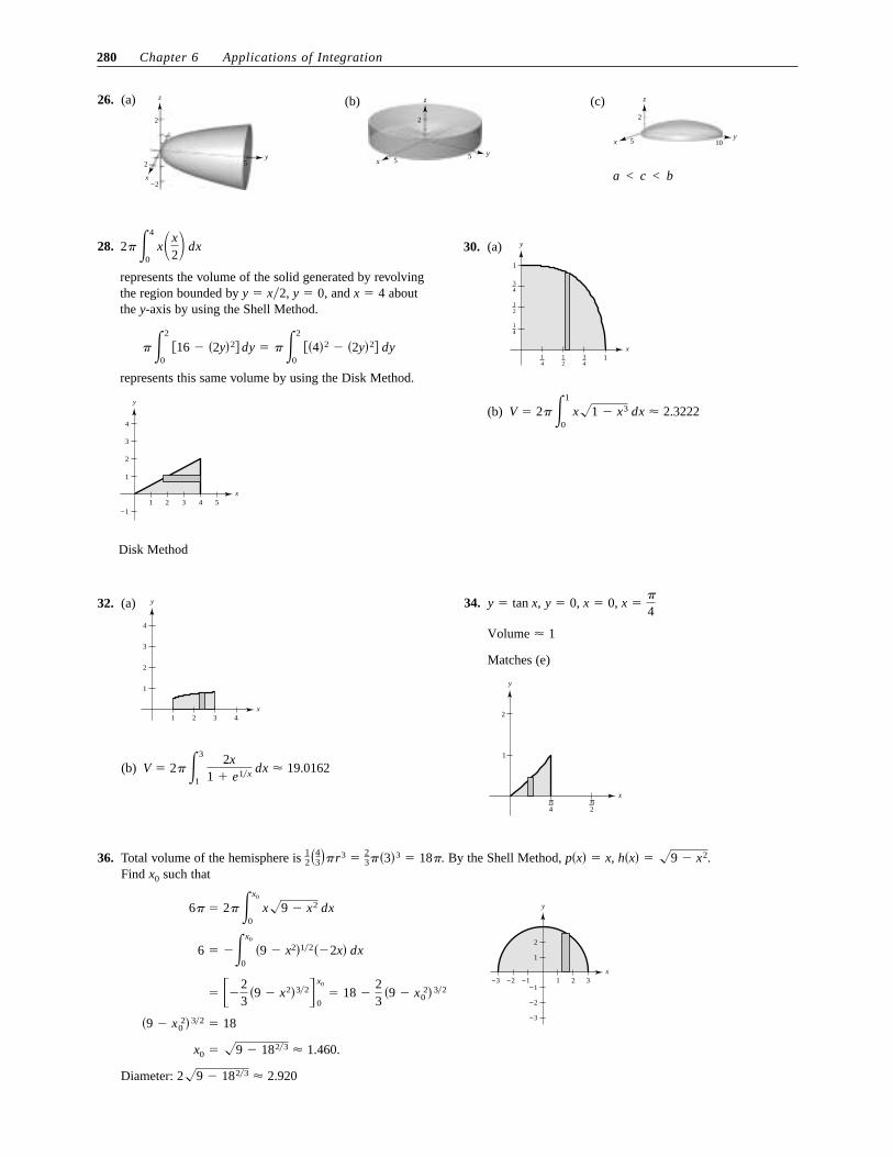
62. The cross sections are squares. By symmetry, we can setup an integral for an eighth of the volume and multiply by 8.
�163
r3
� 8�r2y �13
y3�r
0
V � 8�r
0�r2 � y2� dy
A�y� � b2 � ��r2 � y2�2y
x
(c)
4 − x22
V ��
2�2
�2�4 � x2� dx �
�
2 �4x �x3
3 �2
�2�
16�
3
��
2��4 � x2 �2
��
2�4 � x2�
A�x� �12
�r2 (d)
4 − x2
4 − x2
2
V � �2
�2�4 � x2� dx � �4x �
x3
3 �2
�2�
323
�12
�2�4 � x2 ���4 � x2 � � 4 � x2
A�x� �12
bh
60. —CONTINUED—
64.
�43
� �R2 � r2�3�2
� 2� ��R2 � r2�3�2 ��R2 � r2�3�2
3 �
� 2� ��R2 � r2�x �x3
3 ��R2�r2
0
� 2� ��R2�r2
0 �R2 � r2 � x2� dx
V � � ��R2�r2
��R2�r2
���R2 � x2 �2� r2 dx
r
R
RR2 2− r
66. (a) When represents a square.
When represents a circle.
(b)
To approximate the volume of the solid, form n slices, each of whose area is approximated by the integral above. Then sum the volumes of these n slices.
A � 2 �1
�1 �1 � �x�a�1�a dx � 4 �1
0 �1 � xa�1�a dx
�y� � �1 � �x�a�1�a
a � 2: �x�2 � �y�2 � 1
a � 1: �x� � �y� � 1
x
a = 2
a = 1
−1
−1
1
1
y
Section 6.3 Volume: The Shell Method
2.
� 2��1
0 �x � x2� dx � 2��x2
2�
x3
3 �1
0�
�
3
V � 2��1
0 x�1 � x� dx
h�x� � 1 � x
p�x� � x 4.
� 2��2x2 �x4
4 �2
0� 8�
� 2��2
0 �4x � x3� dx
V � 2��2
0 x�4 � x2� dx
h�x� � 8 � �x2 � 4� � 4 � x2
p�x� � x
6.
1−1−3
3
6
9
12
15
18
2 3 4 5 6
y
x
� ��x4
4 �6
0� 324�
V � 2��6
0
12
x3 dx
h�x� �12
x2
p�x� � x 8.
x21−1−2
1
2
3
y
� 2��2x2 �14
x4�2
0� 8�
V � 2��2
0 �4x � x3� dx
h�x� � 4 � x2
p�x� � x
278 Chapter 6 Applications of Integration
12.
� 2���
0 sin x dx � ��2� cos x�
�
0� 4�
V � 2���
0 x �sin x
x � dx
h�x� �sin x
x
1
−1
2
3
x
4π π
2π
43π
yp�x� � x
10.
x
1
2
3
4
−1 1 2 3
y
� 2��2x2 �23
x3�2
0�
16�
3
� 2��2
0 �4x � 2x2� dx
V � 2��2
0 x�4 � 2x� dx
h�x� � 4 � 2x
p�x� � x
14. on
� 2���y2 �y3
3 �0
�2�
8�
3
� 2��0
�2 ��2y � y2� dy
V � 2��0
�2 ��y��2 � y� dy
h�y� � 4 � �2 � y� � 2 � y
��2, 0���p�y� ≥ 0p�y� � �y 16.
� 2��128 � 64� � 128�
� 2��8y2 �y4
4 �4
0
� 2��4
0�16y � y3� dy
V � 2��4
0y�16 � y2� dy
1
−1
−2
−3
−4
2
3
4
4 8 12
y
x
h�y� � 16 � y2
p�y� � y

Section 6.3 Volume: The Shell Method 279
20.
x1 2 3 4
4
5
−2
−1
1
2
3
y
� 2��4x32 �25
x52�4
0�
192�
5
� 2� �4
0 �6x12 � x32� dx
V � 2� �4
0 �6 � x�x dx
h�x� � x
p�x� � 6 � x
22. (a) Disk
� �100�
3 � 1125
� 1� �49615
�
� 100��x�3
�3�5
1
� 100��5
1x�4 dx
V � ��5
1�10
x2 �2
dx
R�x� �10x2 , r�x� � 0
(b) Shell
� 20��ln x �5
1� 20� ln 5
� 20��5
1 1x dx
V � 2��5
1x�10
x2 � dx
R�x� � x, r�x� � 0
(c) Disk
� ��1003x3 �
200x �
5
1�
190415
�
V � ��5
1�102 � �10 �
10x2 �
2
� dx
R�x� � 10, r�x� � 10 �10x2
1−1−2
2
4
6
8
10
2 3 4 5
y
x
24. (a) Disk
� 2� �a3 �95
a3 �97
a3 �13
a3� �32� a3
105
� 2� �a2x �95
a43x53 �97
a23x73 �13
x3�a
0
� 2� �a
0 �a2 � 3a43x23 � 3a23x43 � x2� dx
V � � �a
�a
�a23 � x23�3 dx
r�x� � 0
R�x� � �a23 � x23�32
x
( , 0)a
(0, )a
( , 0)−a
y (b) Same as part a by symmetry
x
( , 0)a
(0, )a
(0, )−a
y
18.
x
1
2
3
4
−1 1 3
y
� 2��4x2 �83
x3 �12
x4�2
0�
16�
3
� 2� �2
0 �8x � 8x2 � 2x3� dx
V � 2� �2
0 �2 � x��4x � 2x2� dx
h�x� � 4x � x2 � x2 � 4x � 2x2
p�x� � 2 � x
280 Chapter 6 Applications of Integration
26. (a)
x
y
2
2 5
−2
z (b)
xy
2
55
z (c)
a < c < b
xy
2
5 10
z
28.
represents the volume of the solid generated by revolvingthe region bounded by and aboutthe y-axis by using the Shell Method.
represents this same volume by using the Disk Method.
Disk Method
x
4
3
2
1
−153 421
y
� �2
0 �16 � �2y�2� dy � � �2
0 ��4�2 � �2y�2� dy
x � 4y � 0,y � x2,
2� �4
0 x�x
2� dx 30. (a)
(b) V � 2� �1
0 x1 � x3 dx � 2.3222
x1
1
1
1
1
1
3
3
4
4
2
2
4
4
y
32. (a)
(b) V � 2� �3
1
2x1 � e1x dx � 19.0162
x1 2 3 4
4
3
2
1
y 34.
Matches (e)
x
2
1
4π
2π
y
Volume � 1
x ��
4x � 0,y � 0,y � tan x,
36. Total volume of the hemisphere is By the Shell Method,Find such that
Diameter: 29 � 1823 � 2.920
x0 � 9 � 1823 � 1.460.
�9 � x02� 32 � 18
� ��23
�9 � x2�32�x0
0� 18 �
23
�9 � x02� 32
6 � ��x0
0 �9 � x2�12��2x� dx
x
2
1
321−1−1
−3
−2
−3 −2
y 6� � 2� �x0
0 x9 � x2 dx
x0
h�x� � 9 � x2.p�x� � x,12�4
3��r3 �23� �3�3 � 18�.

Section 6.3 Volume: The Shell Method 281
38.
� 2� 2r2R
� 4� R�� r2
2 � � �2��23��r2 � x2�32�
r
�r
� 4� R �r
�r
r2 � x2 dx � 4� �r
�r
xr2 � x2 dx
V � 4� �r
�r
�R � x�r2 � x2 dx
42. (a)
(b) Top line:
Bottom line:
(Note that Simpson’s Rule is exact for this problem.)
� 121,475 cubic feet
� 2� �26,0003 � � 2� �32,000
3 �
� 2���x3
6� 25x2�
20
0� 2���2x3
3� 40x2�
40
20
� 2� �20
0 ��1
2x2 � 50x� dx � 2� �40
20 ��2x2 � 80x� dx
V � 2� �20
0 x��1
2x � 50� dx � 2� �40
20 x��2x � 80� dx
y � 40 �0 � 40
40 � 20�x � 20� � �2�x � 20� ⇒ y � �2x � 80
y � 50 �40 � 5020 � 0
�x � 0� � �12
x ⇒ y � �12
x � 50
�20�
3�5800� � 121,475 cubic feet
�2� �40�
3�4� �0 � 4�10��45� � 2�20��40� � 4�30��20� � 0�
V � 2� �4
0 x f �x� dx
40. (a)
(b)
limn→�
�abn�b � �
limn→�
R1�n� � limn→�
n
n � 1� 1
R1�n� �
abn�1� nn � 1�
�abn�b �n
n � 1
� abn�1�1 �1
n � 1� � abn�1� nn � 1�
� abn�1 � abn�1
n � 1
� �abn x � axn�1
n � 1�b
0
Area region � �b
0�abn � axn� dx (c) Disk Method:
(d)
(e) As the graph approaches the line x � 1.n →�,
limn→�
��b2��abn� � �
limn→�
R2�n� � limn→�
� nn � 2� � 1
R2�n� �
�abn�2� nn � 2�
��b2��abn� � � nn � 2�
� 2�a�bn�2
2�
bn�2
n � 2� � �abn�2� nn � 2�
� 2�a�bn
2x2 �
xn�2
n � 2�b
0
� 2�a�b
0�xbn � xn�1� dx
V � 2��b
0x�abn � axn� dx
Section 6.4 Arc Length and Surfaces of Revolution
2.
(a)
(b)
s � �7
1 �1 � � 4
3�2
dx � �53
x�7
1� 10
y� �43
y �43
x �23
d � ��7 � 12 � �10 � 22 � 10
�1, 2, �7, 10 4.
�2
27�8232 � 1 � 54.929
� � 227
�1 � 9x32�9
0
s � �9
0
�1 � 9x dx
y� � 3x12, �0, 9
y � 2x32 � 3
6.
� 1032 � 232 � 28.794
� �32
�23
�x23 � 132�27
1
�32�
27
1
�x23 � 1� 23x13� dx
� �27
1�x23 � 1
x23 dx
s � �27
1�1 � � 1
x13�2
dx
y� � x�13, �1, 27
y �32
x23 � 4 8.
� � 110
x5 �1
6x3�2
1�
779240
� 3.246
� �2
1 � 1
2x4 �
12x4� dx
� �2
1 ��1
2x4 �
12x4�
2
dx
s � �b
a
�1 � �y�2 dx
1 � �y�2 � �12
x4 �1
2x4�2
, �1, 2
y� �12
x4 �1
2x4
y �x5
10�
16x3
10.
�12 �ex � e�x�
2
0�
12 �e2 �
1e2� � 3.627
�12
�2
0 �ex � e�x dx
s � �2
0 ��1
2�ex � e�x�
2
dx
1 � �y�2 � �12
�ex � e�x�2
, �0, 2
y� �12
�ex � e�x, �0, 2
y �12
�ex � e�x 12. (a)
−3 2
−5
5
y � x2 � x � 2, �2 ≤ x ≤ 1
(b)
L � �1
�2 �2 � 4x � 4x2 dx
1 � �y�2 � 1 � 4x2 � 4x � 1
y� � 2x � 1
(c) L � 5.653
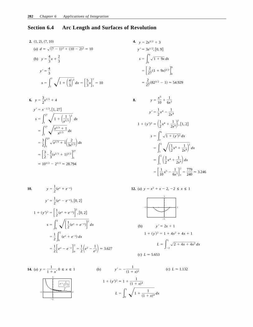
14. (a)
−1 2
−2
y = 1x + 1
5
y �1
1 � x, 0 ≤ x ≤ 1 (b)
L � �1
0 �1 �
1�1 � x4 dx
1 � �y�2 � 1 �1
�1 � x4
y� � �1
�1 � x2(c) L � 1.132
282 Chapter 6 Applications of Integration

16. (a)
−2
−2
2
y x= cos
2
y � cos x, ��
2 ≤ x ≤
�
2(b)
L � ��2
��2 �1 � sin2x dx
1 � �y�2 � 1 � sin2 x
y� � �sin x (c) 3.820
18. (a)
−1 6
−6
2
y � ln x, 1 ≤ x ≤ 5 (b)
L � �5
1 �1 �
1x2 dx
1 � �y�2 � 1 �1x2
y� �1x
(c) L � 4.367
20. (a)
−10
−5
10
10
y � �36 � x 2, 3�3 ≤ x ≤ 6
x � �36 � y2 , 0 ≤ y ≤ 3 (b)
� �3
0
6�36 � y2
dy
L � �3
0 �1 �
y2
36 � y2 dy
��y
�36 � y 2
dxdy
�12
�36 � y2�12��2y (c) L � 3.142 ��!
L � �6
3�3 �1 �
x2
36 � x2 dx � �6
3�3
6�36 � x2
dx
y� �dydx
� �x
�36 � x2
y � �36 � x2
Alternatively, you can convert to a function of x.
Although this integral is undefined at a graphing utility still gives L � 3.142.x � 0,
22.
Matches (e)
s � 1
��4
0 �1 � � d
dx�tan x�
2
dx
x
84
4
2
1
3π
, 1( (
(0, 0)
y x= tan
π
π
y
24.
(a)
(b)
(c)
(d) 160.287
s � �4
0 �1 � �4x�x2 � 4 2 dx � 159.087
� 160.151
d � ��1 � 02 � �9 � 162 � ��2 � 12 � �0 � 92 � ��3 � 22 � �25 � 02 � ��4 � 32 � �144 � 252
d � ��4 � 02 � �144 � 162 � 128.062
f �x � �x2 � 42, �0, 4
Section 6.4 Arc Length and Surfaces of Revolution 283
26. Let and
Equivalently, and
Numerically, both integrals yield L � 2.0035
L2 � �1
0 �1 � e2y dy � �1
0 �1 � e2x dx.
dxdy
� ey,0 ≤ y ≤ 1,x � ey,
L1 � �e
1 �1 �
1x2 dx.y� �
1x
1 ≤ x ≤ e,y � ln x,
28.
Thus, there are square feet of roofing on the barn.100�47 � 4700
�12
�20
�20 �ex20 � e�x20 dx � �10�ex20 � e�x20�
20
�20� 20�e �
1e� � 47 ft
s � �20
�20�� 1
2�ex20 � e�x20�
2
dx
1 � �y�2 � 1 �14
�ex10 � 2 � e�x10 � � 12
�ex20 � e�x20�2
y� � �12
�ex20 � e�x20
y � 31 � 10�ex20 � e�x20
30.
(Use Simpson’s Rule with or a graphing utility.)n � 100
s � �299.2239
�299.2239 �1 � ��0.6899619478 sinh 0.0100333x2 dx � 1480
y� � �0.6899619478 sinh 0.0100333x
y � 693.8597 � 68.7672 cosh 0.0100333x
32.
14
�2��5 � 7.8540 � s
� 5�arcsin 45
� arcsin ��35�� � 7.8540
� �5 arcsin x5�
4
�3
� �4
�3
5�25 � x2
dx
s � �4
�3 � 25
25 � x2 dx
1 � �y�2 �25
25 � x2
y� ��x
�25 � x2
y � �25 � x2 34.
�8�
3�1032 � 532 � 171.258
�83
��x � 132�9
4
� 4��9
4
�x � 1 dx
S � 2��9
42�x�1 �
1x dx
y� �1�x
, �4, 9
y � 2�x
284 Chapter 6 Applications of Integration

36.
� �2��58
x2�6
0� 9�5 �
S � 2� �6
0 x2�5
4 dx
1 � �y�2 �54
, �0, 6
y� �12
y �x2
38.
��
6�3732 � 1 � 117.319
� ��
6�1 � 4x232�
3
0
��
4�3
0�1 � 4x212 �8x dx
S � 2��3
0x�1 � 4x2 dx
y� � �2x
y � 9 � x2, �0, 3
40.
� 2� �e
1 �x2 � 1 dx � 22.943
S � 2� �e
1 x�x2 � 1
x2 dx
1 � �y�2 �x2 � 1
x2 , �1, e
y� �1x
y � ln x 42. The precalculus formula is the distance formula betweentwo points. The representative element is
���xi2 � ��yi2 ��1 � ��yi
�xi�2
�xi.
44. The surface of revolution given by will be larger. is larger for f1.r�xf1
46.
� 2� �r
�r
r dx � �2� rx�r
�r� 4� r2
S � 2� �r
�r
�r2 � x2� r2
r2 � x2 dx
1 � �y�2 �r2
r2 � x2
y� ��x
�r2 � x2
y � �r2 � x2 48. From Exercise 47 we have:
x
x y r2 2 2+ =
r
r h−
h
y
� 2�rh �where h is the height of the zone
� 2r� �r � �r2 � a2 � 2r2� � 2r��r2 � a2
� ��2r��r2 � x2�a
0
� �r� �a
0
�2x dx�r2 � x2
S � 2� �a
0
rx�r2 � x2
dx
Section 6.4 Arc Length and Surfaces of Revolution 285

50. (a) We approximate the volume by summing 6 disks of thickness 3 and circumference equal to the average of the given circumferences:
(b) The lateral surface area of a frustum of a right circular cone is For the first frustum,
Adding the six frustums together,
� 1168.64
� 224.30 � 208.96 � 208.54 � 202.06 � 174.41 � 150.37
�58 � 512 ��9 � � 7
2��2
�12
� �51 � 482 ��9 � � 3
2��2
�12
�70 � 662 ��9 � � 4
2��2
�12
� �66 � 582 ��9 � � 8
2��2
�12
�
S � �50 � 65.52 ��9 � �15.5
2� �2
�12
� �65.5 � 702 ��9 � �4.5
2��2
�12
�
� �50 � 65.52 ��9 � �65.5 � 50
2� �2
�12
.
r
R
sh
S1 � ��32 � �65.5 � 502� �
2
�12
� 502�
�65.52� �
�s�R � r.
�3
4��21813.625 � 5207.62 cubic inches
�3
4��57.752 � 67.752 � 682 � 622 � 54.52 � 49.52
�3
4� ��50 � 65.52 �
2
� �65.5 � 702 �
2
� �70 � 662 �
2
� �66 � 582 �
2
� �58 � 512 �
2
� �51 � 482 �
2
�
V � �6
i�1� ri
2�3 � �6
i�1�� Ci
2��2
�3 �3
4� �
6
i�1Ci
2
Ci
(c)
−1
−1 19
20
r � 0.00401y3 � 0.1416y2 � 1.232y � 7.943 (d)
� 1179.5 square inches
S � �18
0 2�r�y�1 � r��y2 dy
V � �18
0 �r2 dy � 5275.9 cubic inches
52. Individual project, see Exercise 50, 51.
(c) You cannot evaluate this definite integral, since the integrand is not defined at Simpson’s Rule will not work for thesame reason. Also, the integrand does not have an elementary antiderivative.
x � 3.
56. Essay
54. (a)
Ellipse:
−5 5
−4 9x2 2y
4+ = 1
4
y2 � �2�1 �x2
9
y1 � 2�1 �x2
9
x2
9�
y2
4� 1 (b)
L � �3
0�1 �
4x2
81 � 9x2 dx
��2x
9�1 �x2
9
��2x
3�9 � x2
y� � 2�12��1 �
x2
9 ��12
��2x9 �
y � 2�1 �x2
9, 0 ≤ x ≤ 3
286 Chapter 6 Applications of Integration
Section 6.5 Work
Section 6.5 Work 287
2. W � Fd � �2800��4� � 11,200 ft � lb 4. W � Fd � �9�2000��� 12 �5280�� � 47,520,000 ft � lb
6. is the work done by a force F moving an object along a straight line from to x � b.x � aW � �b
a
F�x� dx
8. (a)
(b)
(c)
(d) W � �9
0 �x dx �
23
x3�29
0�
23
�27� � 18 ft � lbs
W � �9
0
127
x2 dx �x3
819
0� 9 ft � lbs
� 160 ft � lbs
W � �7
0 20 dx � �9
7 ��10x � 90� dx � 140 � 20
W � �9
0 6 dx � 54 ft � lbs 10.
� 40 in � lb 3.33 ft � lb
W � �10
0 54
x dx � �58
x210
6
12.
� 28000 n � cm � 280 Nm
W � �70
0 F�x� dx � �70
0 807
x dx �40x2
7 70
0
800 � k�70� ⇒ k �807
F�x� � kx 14.
� 240 ft � lb
W � 2 �4
0 15x dx � �15x2
4
0
15 � k�1� � k
F�x� � kx
16.
W � �5�24
1�6 540x dx � 270x2
5�24
1�6� 4.21875 ft � lbs
W � 7.5 � �1�6
0 kx dx �
kx2
2 1�6
0�
k72
⇒ k � 540 18.
limh→�
W � 20,000 mi�ton 2.1 � 1011 ft � lb
��80,000,000
h� 20,000
W � �h
4000
80,000,000x2 dx � ��
80,000,000x
h
4000
20. Weight on surface of moon:
Weight varies inversely as the square of distance from the center of the moon. Therefore,
95.652 mi � ton 1.01 � 109 ft � lb
W � �1150
1100 2.42 � 106
x2 dx � ��2.42 � 106
x 1150
1100� 2.42 � 106� 1
1100�
11150
k � 2.42 � 106
2 �k
�1100�2
F�x� �kx2
16 �12� � 2 tons
22. The bottom half had to be pumped a greater distance then the top half.
24. Volume of disk:
Weight of disk:
Distance the disk of water is moved: y
� 862,400� newton–meters
� 39,200� �22�
W � �12
10y�9800��4�� dy � 39,200� �y2
2 12
10
9800�4�� y
4� y
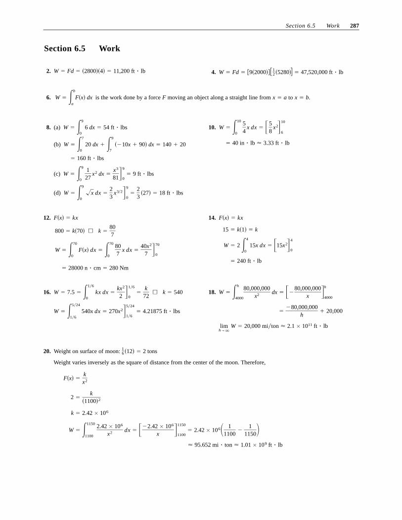
26. Volume of disk:
Weight of disk:
Distance:
(a)
(b) W �49
�62.4�� �6
4 y3 dy � �4
9�62.4���1
4y4
6
4 7210.7� ft � lb
W �49
�62.4�� �2
0 y3 dy � �4
9�62.4���1
4y4
2
0 110.9� ft � lb
y
62.4��23
y 2
y
�� 23
y 2
y
x
y
4321−1−2−3−4
7
5
4
3
2
y
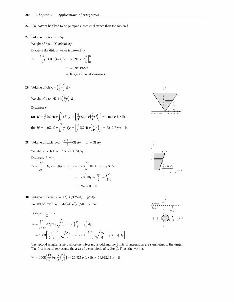
28. Volume of each layer:
Weight of each layer:
Distance:
� 3252.6 ft � lb
� 55.6�18y �3y2
2�
y3
3 3
0
W � �3
055.6�6 � y��y � 3� dy � 55.6�3
0�18 � 3y � y2� dy
6 � y
55.6�y � 3� y
x1 2 3 4
4
3
2
1
(2, 3)
y x= 3 3−
yy � 3
3�3� y � �y � 3� y
30. Volume of layer:
Weight of layer:
Distance:
The second integral is zero since the integrand is odd and the limits of integration are symmetric to the origin. The first integral represents the area of a semicircle of radius Thus, the work is
W � 1008�192 ��5
2 2
�12 � 29,925� ft � lb 94,012.16 ft � lb.
52 .
� 1008�192
�2.5
�2.5 �25
4� y2 dy � �2.5
�2.5 �25
4� y2 ��y� dy
W � �2.5
�2.5 42�24��25
4� y2 �19
2� y dy
192
� y
W � 42�24���25�4� � y2 y
V � 12�2���25�4� � y2 y
x
6
3
12
963−3−3
−6
−9 −6
192
− y
Ground
level
y
288 Chapter 6 Applications of Integration

32. The lower 10 feet of chain are raised 5 feet with a constant force.
The top 5 feet will be raised with variable force.
Weight of section:
Distance:
W � W1 � W2 � 150 �752
�3752
ft � lb
W2 � 3 �5
0 �5 � y� dy � ��3
2�5 � y�2
5
0�
752
ft � lb
5 � y
3 y
W1 � 3�10�5 � 150 ft � lb
34. The work required to lift the chain is (from Exercise 31). The work required to lift the 500-pound load isThe work required to lift the chain with a 100-pound load attached is
W � 337.5 � 7500 � 7837.5 ft � lbs
W � �500��15� � 7500.337.5 ft � lb
36. W � 3 �6
0 �12 � 2y� dy � ��3
4�12 � 2y�2
6
0�
34
�12�2 � 108 ft � lb
38. Work to pull up the ball:
Work to pull up the cable: force is variable
Weight per section:
Distance:
W � W1 � W2 � 20,000 � 800 � 20,800 ft � lb
� 800 ft � lb
W2 � �40
0 �40 � x� dx � ��1
2�40 � x�2
40
0
40 � x
1 y
W1 � 500�40� � 20,000 ft � lb 40.
� 2500 ln 3 2746.53 ft � lb
W � �3
1 2500
V dV � �2500 ln V
3
1
2500 �k1
⇒ k � 2500
p �kV
42. (a)
(b)
24,88.889 ft � lb
W 2 � 03�6� �0 � 4�20,000� � 2�22,000� � 4�15,000� � 2�10,000� � 4�5000� � 0�
W � FD � �8000���2� � 16,000� ft � lbs
(c)
(d) when is a maximum when feet.
(e) W � �2
0 F�x� dx 25,180.5 ft � lbs
x 0.524F�x�x 0.524 feet.F�x� � 0
0 20
25,000
F�x� � �16,261.36x4 � 85,295.45x3 � 157,738.64x2 � 104,386.36x � 32.4675
44. W � �4
0 �ex2
� 1100 dx 11,494 ft � lb 46. W � �2
0 1000 sinh x dx 2762.2 ft � lb
Section 6.5 Work 289
Section 6.6 Moments, Centers of Mass, and Centroids
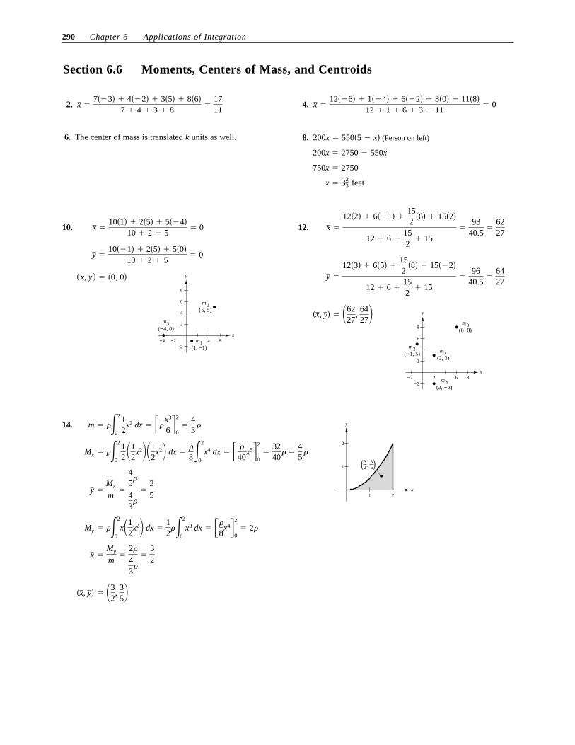
2. x �7��3� � 4��2� � 3�5� � 8�6�
7 � 4 � 3 � 8�
1711
4. x �12��6� � 1��4� � 6��2� � 3�0� � 11�8�
12 � 1 � 6 � 3 � 11� 0
6. The center of mass is translated k units as well. 8. (Person on left)
x � 323 feet
750x � 2750
200x � 2750 � 550x
200x � 550�5 � x�
10.
xm1
m2
m3
(1, 1)−
(5, 5)
( 4, 0)−
−4 −2−2
4 6
8
6
4
2
y �x, y � � �0, 0�
y �10��1� � 2�5� � 5�0�
10 � 2 � 5� 0
x �10�1� � 2�5� � 5��4�
10 � 2 � 5� 0 12.
x
m1
m4
m3
m2
(2, 3)
(2, 2)−
(6, 8)
( 1, 5)−
−2−2
2 6 8
8
6
2
y �x, y� � �6227
, 6427�
y �
12�3� � 6�5� �152
�8� � 15��2�
12 � 6 �152
� 15�
9640.5
�6427
x �
12�2� � 6��1� �152
�6� � 15�2�
12 � 6 �152
� 15�
9340.5
�6227
14.
�x, y� � �32
, 35�
x �My
m�
2�
43
�
�3
2
My � ��2
0x�1
2x2� dx �
12
��2
0x3 dx � ��
8x4�
2
0� 2�
y �Mx
m�
45
�
43
�
�3
5
Mx � ��2
0
12 �
12
x2��12
x2� dx ��
8�2
0x4 dx � � �
40x5�
2
0�
3240
� �45
�
y
x1
1
2
2
32
35
,( )
m � ��2
0
12
x2 dx � ��x3
6 �2
0�
43
�
290 Chapter 6 Applications of Integration
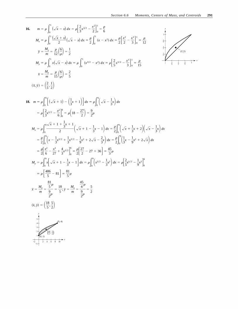
16.
�x, y � � �25
, 12�
x �My
m�
�
15 �6�� �
25
My � � �1
0 x�x � x� dx � � �1
0 �x32 � x2� dx � ��2
5x52 �
x3
3 �1
0�
�
15
y �Mx
m�
�
12 �6�� �
12
Mx � � �1
0 �x � x�
2�x � x� dx �
�
2 �1
0 �x � x2� dx �
�
2 �x2
2�
x3
3 �1
0�
�
12
m � � �1
0 �x � x� dx � ��2
3x32 �
x2
2�1
0�
�
6
x1
1
14
14
12
34
34
12
( , )x y
y
18.
2−2−1
1
2
3
4
5
4 6 8 10
y
x
185
52
,( )
(9, 4)
(0, 1)
�x, y� � �185
, 52�
x �My
m�
815
�
92
�
�18
5; y �
Mx
m�
454
�
92
�
�5
2
� � �4865
� 81� �815
�
My � ��9
0x�x � 1 �
13
x � 1� dx � ��9
0�x32 �
13
x2� dx � ��25
x52 �19
x3�9
0
��
2�x2
6�
x3
27�
43
x32�9
0�
�
2�272
� 27 � 36� �453
�
��
2�9
0�x �
13
x32 �13
x32 �19
x2 � 2x �23
x� dx ��
2�9
0�1
3x �
19
x2 � 2x� dx
Mx � ��9
0
x � 1 �13
x � 1
2 �x � 1 �13
x � 1� dx ��
2�9
0�x �
13
x � 2��x �13
x� dx
� ��23
x32 �x2
6 �9
0� ��18 �
272 � �
92
�
m � ��9
0��x � 1� � �1
3x � 1�� dx � ��9
0�x �
13
x� dx
Section 6.6 Moments, Centers of Mass, and Centroids 291
x
−4
−4−8
12
4
8
8
( , )x y
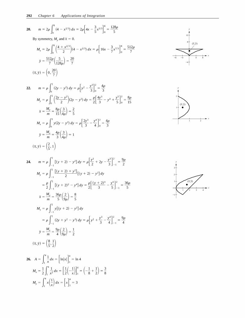
y20.
By symmetry, and
�x, y � � �0, 207 �
y �512�
7 � 5128�� �
207
Mx � 2� �8
0 �4 � x23
2 ��4 � x23� dx � ��16x �37
x73�8
0�
512�
7
x � 0.My
m � 2� �8
0 �4 � x23� dx � 2��4x �
35
x53�8
0�
128�
5
x1 2
1
2
( , )x y
y22.
�x, y � � �25
, 1�
y �Mx
m�
4�
3 � 34�� � 1
Mx � � �2
0 y�2y � y2� dy � ��2y3
3�
y4
4 �2
0�
4�
3
x �My
m�
8�
15 �34�� �
25
My � � �2
0 �2y � y2
2 ��2y � y2� dy ��
2�4y3
3� y4 �
y5
5 �2
0�
8�
15
m � � �2
0 �2y � y2� dy � ��y2 �
y3
3�2
0�
4�
3
1
1
−1
2
2
3
3 4x
( , )x y
y24.
�x, y � � �85
, 12�
y �Mx
m�
9�
4 � 29�� �
12
� � �2
�1 �2y � y2 � y3� dy � ��y2 �
y3
3�
y4
4 �2
�1�
9�
4
Mx � � �2
�1 y ��y � 2� � y2� dy
x �My
m�
36�
5 � 29�� �
85
��
2 �2
�1 ��y � 2�2 � y4� dy �
�
2��y � 2�3
3�
y5
5 �2
�1�
36�
5
My � � �2
�1 ��y � 2� � y2�
2��y � 2� � y2� dy
m � � �2
�1 ��y � 2� � y2� dy � ��y2
2� 2y �
y3
3 �2
�1�
9�
2
26.
My � �4
1 x�1
x� dx � �x�4
1� 3
Mx �12
�4
1 1x2 dx � �1
2 ��1x��
4
1� ��1
8�
12� �
38
A � �4
1 1x dx � �ln x �
4
1� ln 4
292 Chapter 6 Applications of Integration
28.
by symmetry.My � 0
� �12�
x5
5�
8x3
3� 16x�
2
�2� ��32
5�
643
� 32� � �25615
Mx �12
�2
�2 �x2 � 4��4 � x2� dx � �
12
�2
�2 �x4 � 8x2 � 16� dx
A � �2
�2 ��x2 � 4� dx � 2 �2
0 �4 � x2� dx � �8x �
2x3
3 �2
0� 16 �
163
�323
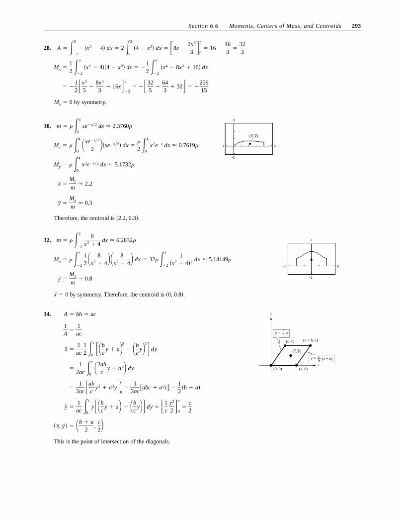
30.
Therefore, the centroid is �2.2, 0.3�.
y �Mx
m� 0.3
x �My
m� 2.2
My � � �4
0 x2e�x2 dx � 5.1732�
Mx � � �4
0 �xe�x2
2 ��xe�x2� dx ��
2 �4
0 x2e�x dx � 0.7619�
m � � �4
0 xe�x2 dx � 2.3760�
−1
−1
5
( , )x y
3
32.
by symmetry. Therefore, the centroid is �0, 0.8�.x � 0
y �Mx
m� 0.8
Mx � � �2
�2 12 �
8x2 � 4��
8x2 � 4� dx � 32� �2
�2
1�x2 � 4�2 dx � 5.14149�
−3 3
−1
3m � � �2
�2
8x2 � 4
dx � 6.2832�
34.
This is the point of intersection of the diagonals.
�x, y � � �b � a2
, c2�
y �1ac
�c
0 y��b
cy � a� � �b
cy�� dy � �1
c y2
2 �c
0�
c2
�1
2ac�abc
y2 � a2y�c
0�
12ac
�abc � a2c� �12
�b � a�
�1
2ac �c
0 �2ab
cy � a2� dy
x �1ac
12
�c
0 ��b
cy � a�
2
� �bc
y�2
� dy
1A
�1ac
x
( , )x y
y = cb
x
cb ( )x a−y =
(0, 0)
( , )b c
( , 0)a
( + , )a b c
yA � bh � ac
Section 6.6 Moments, Centers of Mass, and Centroids 293
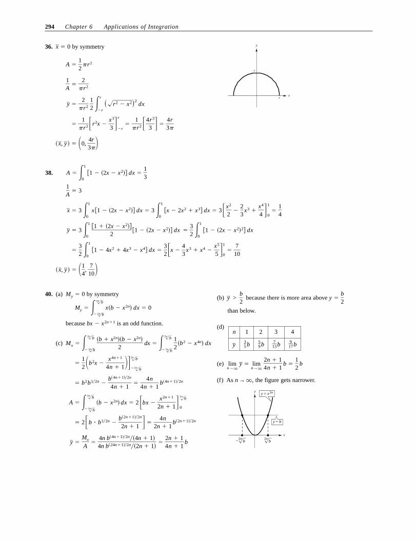
(b) because there is more area above
than below.
(d)
(e)
(f) As the figure gets narrower.
x
y b=
y x= 2n
b−2nb
2n
y
n →�,
limn→�
y � limn→�
2n � 14n � 1
b �12
b
y �b2
y > b2
40. (a) by symmetry
because is an odd function.
(c)
y �Mx
A�
4n b�4n�1�2n�4n � 1�4n b�24n�1�2n�2n � 1� �
2n � 14n � 1
b
� 2�b � b12n �b�2n�1�2n
2n � 1 � �4n
2n � 1b�2n�1�2n
A � � 2nb
�2nb
�b � x2n� dx � 2 �bx �x2n�1
2n � 1�2nb
0
� b2b12n �b�4n�1�2n
4n � 1�
4n4n � 1
b�4n�1�2n
�12 �b2x �
x4n�1
4n � 1��2nb
�2nb
Mx � � 2nb
�2nb
�b � x2n��b � x2n�
2 dx � � 2nb
�2nb
12
�b2 � x4n� dx
bx � x2n�1
My � � 2nb
�2nb
x�b � x2n� dx � 0
My � 0
36. by symmetry
�x, y � � �0, 4r3��
�1
�r2�r2x �x3
3�r
�r�
1�r2 �4r3
3 � �4r3�
y �2
�r2 12
�r
�r
�r2 � x2�2 dx
1A
�2
�r2
A �12
�r2
x � 0
r
r
x
y
38.
�x, y � � �14
, 710�
�32
�1
0 �1 � 4x2 � 4x3 � x4� dx �
32�x �
43
x3 � x4 �x5
5 �1
0�
710
�32
�1
0 �1 � �2x � x2�2� dx y � 3 �1
0 �1 � �2x � x2��
2�1 � �2x � x2�� dx
x � 3 �1
0 x �1 � �2x � x2�� dx � 3 �1
0 �x � 2x2 � x3� dx � 3�x2
2�
23
x3 �x4
4 �1
0�
14
1A
� 3
A � �1
0 �1 � �2x � x2�� dx �
13
n 1 2 3 4
917 b7
13 b59 b3
5 by
294 Chapter 6 Applications of Integration

42. Let be the top curve, given by The bottom curve is
(a)
�x, y � � �0, 1.078�
y �Mx
A�
4.97974.62
� 1.078
�16
�29.878� � 4.9797
f
d
−2 20
3 �2
3�4� �3.75 � 4�3.4945� � 2�2.808� � 4�1.6335� � 0�
� �2
0 � f �x�2 � d�x�2� dx
Mx � �2
�2 f �x� � d�x�
2� f �x� � d�x�� dx
�13
�13.86� � 4.62
� 22
3�4� �1.50 � 4�1.45� � 2�1.30� � 4�.99� � 0�
Area � 2 �2
0 � f �x� � d�x�� dx
d�x�.l � d.f �x�
x 0 0.5 1.5 2.0
f 2.0 1.93 1.73 1.32 0
d 0.50 0.48 0.43 0.33 0
1.0
(b)
(c)
�x, y � � �0, 1.068�
y �Mx
A�
4.91334.59998
� 1.068
d�x� � �0.02648x4 � 0.01497x2 � .4862
f �x� � �0.1061x4 � 0.06126x2 � 1.9527
44. Centroids of the given regions: and
Area:
�x, y � � �2514
, 1514�
y �3�32� � 2�12� � 2�1�
7�
1527
�1514
x �3�12� � 2�2� � 2�72�
7�
2527
�2514
A � 3 � 2 � 2 � 7
�72
, 1��12
, 32�, �2,
12�,
x
1
2
3
4
41 2 3
m1m3m2
y
46.
By symmetry,
�x, y � � �0, 55232128� � �0, 2.595�
y ��74��716� � �28764��5516�
�74� � �28764� �16,5696384
�55232128
x � 0.
m2 �78 �6 �
78� �
28764
, P2 � �0, 5516�
m1 �78
�2� �74
, P1 � �0, 7
16�
x1
2
3
4
5
−1 12
32
32
− 12
−
m1
m2
y
Section 6.6 Moments, Centers of Mass, and Centroids 295

48. Centroids of the given regions: and
Mass:
�x, y � � �8 � 3�
8 � �, 0� � �1.56, 0�
x �8�1� � ��3�
8 � ��
8 � 3�
8 � �
y � 0
8 � �
�1, 0��3, 0� 50. V � 2�rA � 2��3��4�� � 24�2
52.
V � 2�rA � 2��225 ��32
3 � �1408�
15� 294.89
r � x �225
x �My
A�
70415
323�
22
5
� 2�645
�323 � �
70415
My � 2�4
0�u � 2�u du � 2�4
0�u32 � 2u12� du � 2�2
5u52 �
43
u32�4
0
Let u � x � 2, x � u � 2, du � dx:
My � �6
2�x�2x � 2 dx � 2�6
2xx � 2 dx
2
2
4
6
4 6
y
x
(6, 4)
( , )x y
A � �6
22x � 2 dx �
43
�x � 2�32�6
2�
323
54. A planar lamina is a thin flat plate of constant density. The center of mass is the balancing point on the lamina.
�x, y�
56. Let R be a region in a plane and let L be a line such that L does not intersect the interiorof R. If r is the distance between the centroid of R and L, then the volume V of the solid of revolution formed by revolving R about L is
where A is the area of R.
V � 2�rA
58. The centroid of the circle is The distance traveled by the centroid is The arc length of the circle is also Therefore,
x
−2
−1
−1 1
1
3
2
d
C
y
S � �2���2�� � 4�2.2�.2�.�1, 0�.
296 Chapter 6 Applications of Integration
Section 6.7 Fluid Pressure and Fluid Force
Section 6.7 Fluid Pressure and Fluid Force 297
2. F � PA � �62.4�5���16� � 4992 lb 4.
� 62.4�4��48� � 11,980.8 lb
F � 62.4�h � 4��48� � �62.4��h��48�
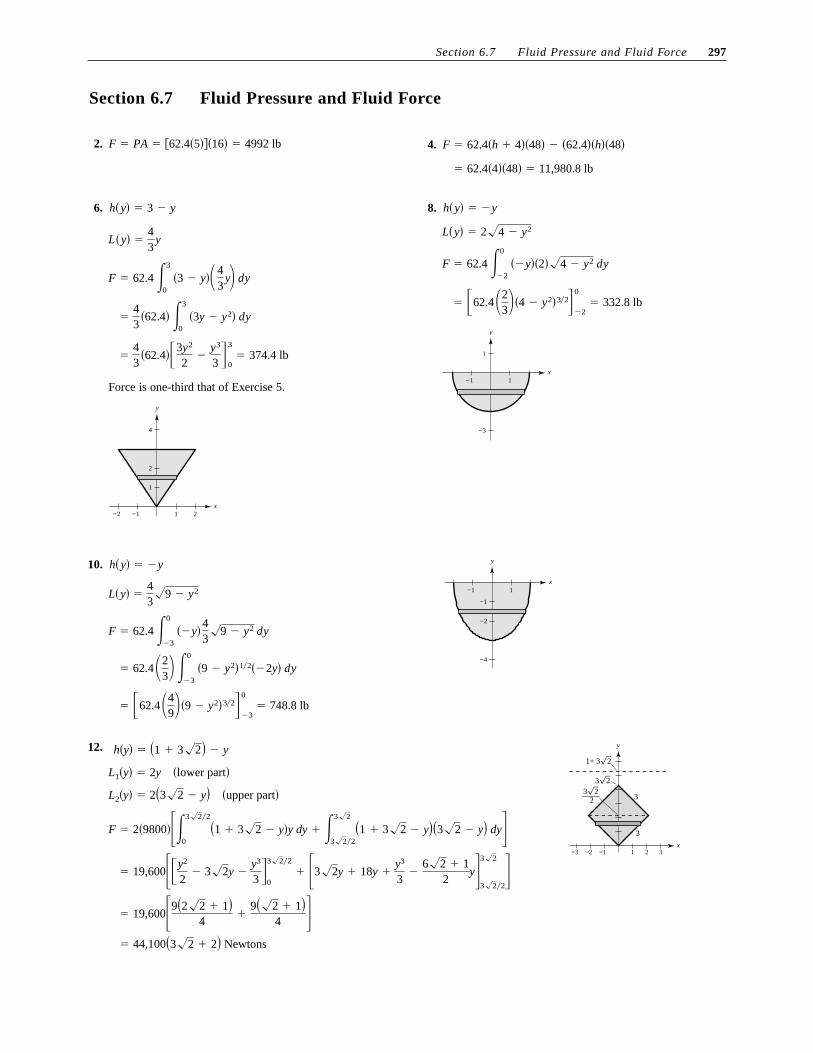
6.
Force is one-third that of Exercise 5.
x1−1−2 2
4
2
1
y
�43
�62.4��3y2
2�
y3
3 �3
0� 374.4 lb
�43
�62.4� �3
0 �3y � y2� dy
F � 62.4 �3
0 �3 � y� 4
3y dy
L�y� �43
y
h�y� � 3 � y 8.
x1−1
−3
1
y
� �62.423�4 � y2�3�2�
0
�2� 332.8 lb
F � 62.4 �0
�2 ��y��2��4 � y2 dy
L�y� � 2�4 � y2
h�y� � �y
10.
� �62.449�9 � y2�3�2�
0
�3� 748.8 lb
� 62.423 �0
�3 �9 � y2�1�2��2y� dy
F � 62.4 �0
�3 ��y� 4
3�9 � y2 dy
L�y� �43�9 � y2
h�y� � �yx
1−1
−1
−2
−4
y
12.
� 44,100�3�2 � 2� Newtons
� 19,600�9�2�2 � 1�4
�9��2 � 1�
4 � � 19,600��y2
2� 3�2y �
y3
3 �3�2�2
0� �3�2y � 18y �
y3
3�
6�2 � 12
y�3�2
3�2�2�
F � 2�9800���3�2�2
0�1 � 3�2 � y�y dy � �3�2
3�2�2�1 � 3�2 � y��3�2 � y� dy�
L2�y� � 2�3�2 � y� �upper part�
L1�y� � 2y �lower part�23
23
2 1+ 3
2
3
3
y
x1−1−2−3 2 3
h�y� � �1 � 3�2� � y
298 Chapter 6 Applications of Integration
14.
x−3 −2 −1 1 2 3
6
y
� 9800�6y �y2
2 �5
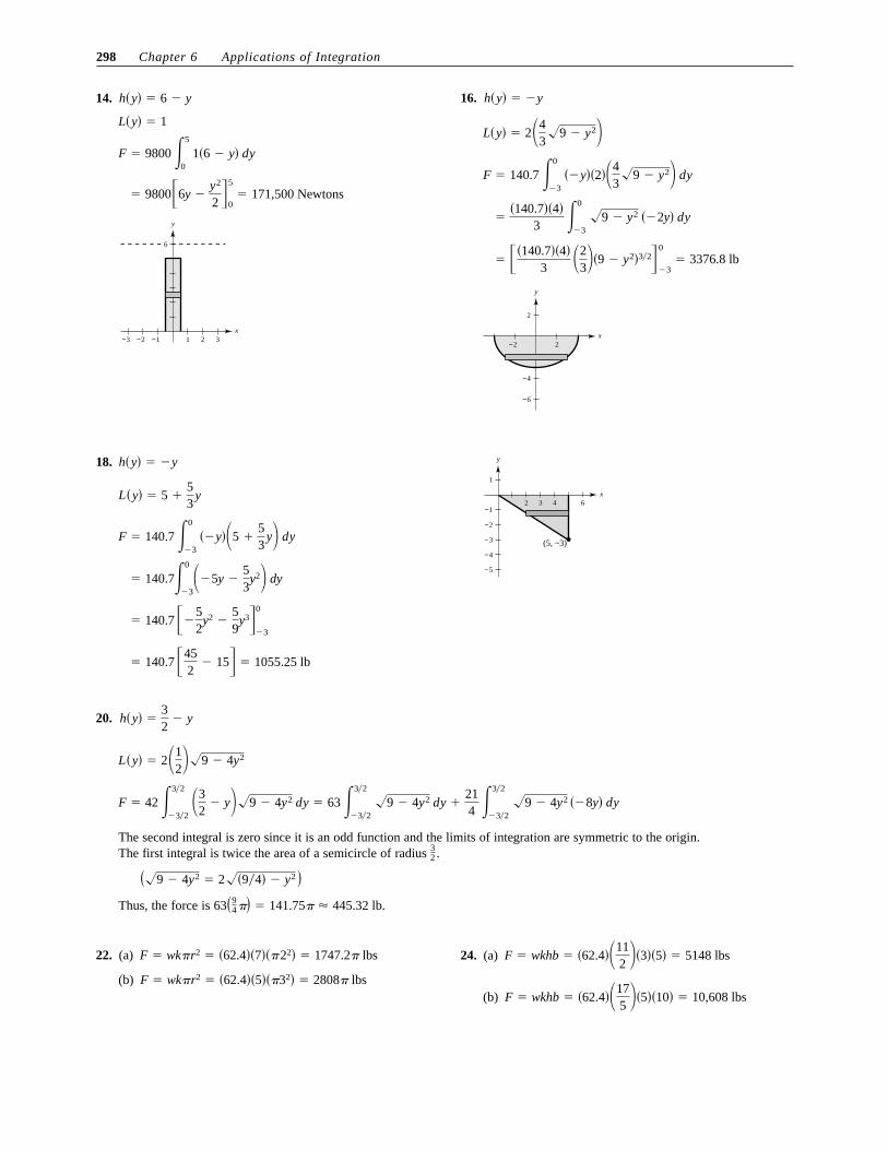
0� 171,500 Newtons
F � 9800 �5
0 1�6 � y� dy
L�y� � 1
h�y� � 6 � y 16.
x2−2
−6
−4
2
y
� ��140.7��4�3 2
3�9 � y2�3�2�0
�3� 3376.8 lb
��140.7��4�
3 �0
�3 �9 � y2 ��2y� dy
F � 140.7 �0
�3 ��y��2�4
3�9 � y2 dy
L�y� � 243�9 � y2
h�y� � �y
18.
� 140.7 �452
� 15� � 1055.25 lb
� 140.7 ��52
y2 �59
y3�0
�3
� 140.7�0
�3�5y �
53
y2 dy
F � 140.7 �0
�3 ��y�5 �
53
y dy
L�y� � 5 �53
y
h�y� � �y
x2 3 4 6
−1
−2
−3
−4
−5
1
y
(5, −3)
20.
The second integral is zero since it is an odd function and the limits of integration are symmetric to the origin. The first integral is twice the area of a semicircle of radius
Thus, the force is 63�94 �� � 141.75� 445.32 lb.
��9 � 4y2 � 2��9�4� � y2 �
32 .
F � 42 �3�2
�3�2 3
2� y�9 � 4y2 dy � 63 �3�2
�3�2 �9 � 4y2 dy �
214
�3�2
�3�2 �9 � 4y2 ��8y� dy
L�y� � 212�9 � 4y2
h�y� �32
� y
22. (a)
(b) F � wk�r2 � �62.4��5���32� � 2808� lbs
F � wk�r2 � �62.4��7���22� � 1747.2� lbs 24. (a)
(b) F � wkhb � �62.4�175 �5��10� � 10,608 lbs
F � wkhb � �62.4�112 �3��5� � 5148 lbs
Review Exercises for Chapter 6
26. From Exercise 21:
F � 64�15���12�
2
� 753.98 lb
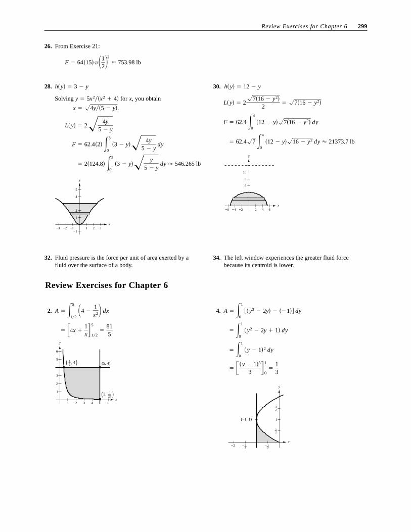
28.
Solving for x, you obtain
x
2
4
1
5
321−1−1
−3 −2
y
� 2�124.8� �3
0 �3 � y�� y
5 � y dy � 546.265 lb
F � 62.4�2� �3
0 �3 � y�� 4y
5 � y dy
L�y� � 2� 4y5 � y
x � �4y�5 � y�.y � 5x2�x2 � 4�
h�y� � 3 � y 30.
x−6 −4 −2 2 4 6
10
8
6
y
� 62.4�7 �4
0 �12 � y��16 � y2 dy � 21373.7 lb
F � 62.4 �4
0 �12 � y��7�16 � y2� dy
L�y� � 2�7�16 � y2�
2� �7�16 � y2�
h�y� � 12 � y
32. Fluid pressure is the force per unit of area exerted by afluid over the surface of a body.
34. The left window experiences the greater fluid forcebecause its centroid is lower.
Review Exercises for Chapter 6 299
2.
x1 2 3 4
1
2
3
5
6
6
(5, 4)
5, 125( )
12
, 4 )(
y
� 4x �1x�
5
12�
815
A � �5
12 �4 �
1x2� dx 4.
( 1, 1)−
x
1
−2
12
32
32
− 12
−
y
� �y � 1�3
3 �1
0�
13
� �1
0 �y � 1�2 dy
� �1
0 �y2 � 2y � 1� dy
A � �1
0 ��y2 � 2y� � ��1� dy
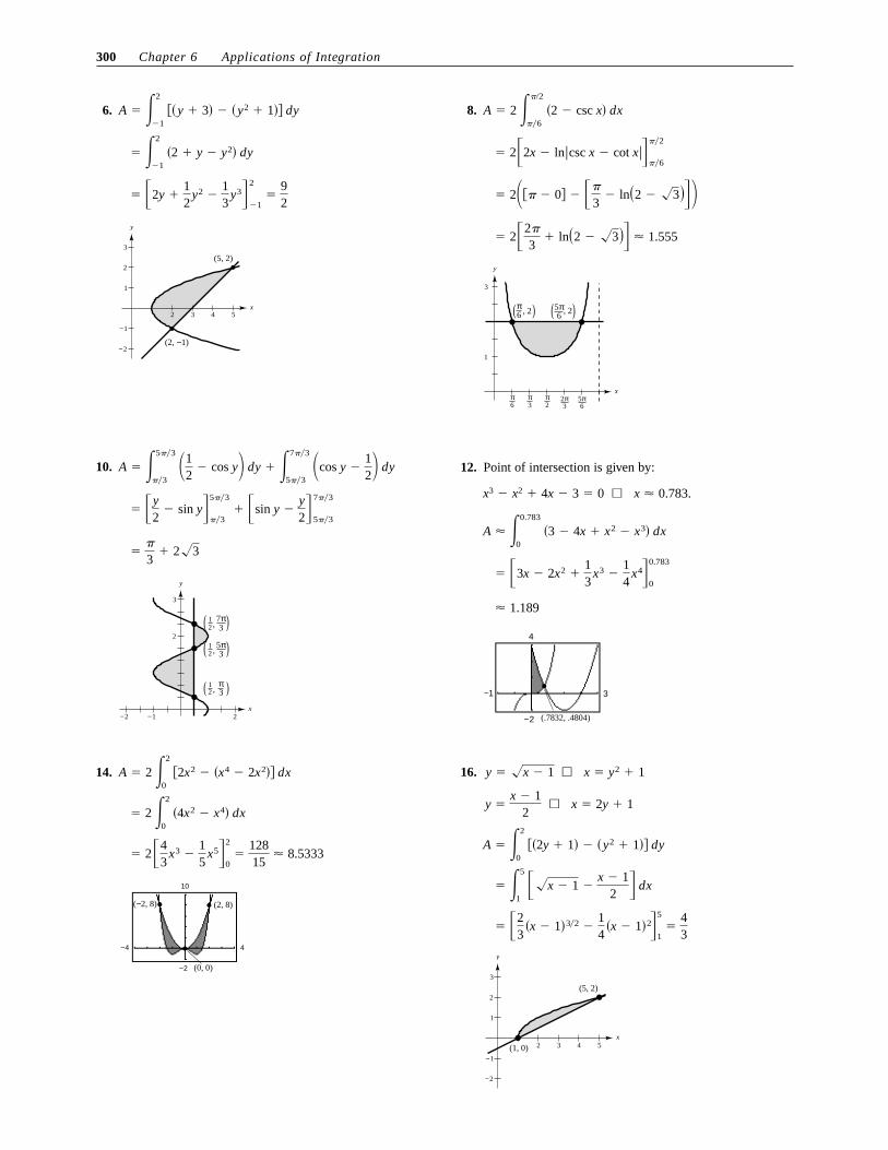
300 Chapter 6 Applications of Integration
6.
x
−1
−2
1
2
3
2 3 4 5
(2, 1)−
(5, 2)
y
� 2y �12
y2 �13
y3�2
�1�
92
� �2
�1 �2 � y � y2� dy
A � �2
�1 ��y � 3� � �y2 � 1� dy 8.
3
1
xπ2
π3
π6
2π3
5π6
π6 , 2( ) 5π
6, 2( )
y
� 22�
3� ln�2 � �3�� � 1.555
� 2��� � 0 � �
3� ln�2 � �3���
� 22x � ln�csc x � cot x���2
�6
A � 2 ���2
�6 �2 � csc x� dx
10.
x−2 −1 2
2
3
12
12
12 3
5π
37π
π3
,
,
,
(
(
(
)
)
)
y
��
3� 2�3
� y2
� sin y�5�3
�3� sin y �
y2�
7�3
5�3
A � �5�3
�3 �1
2� cos y� dy � �7�3
5�3 �cos y �
12� dy 12. Point of intersection is given by:
(.7832, .4804)
−1 3
−2
4
� 1.189
� 3x � 2x2 �13
x3 �14
x4�0.783
0
A � �0.783
0 �3 � 4x � x2 � x3� dx
x3 � x2 � 4x � 3 � 0 ⇒ x � 0.783.
14.
( 2, 8)−
(0, 0)
(2, 8)
−4 4
−2
10
� 243
x3 �15
x5�2
0�
12815
� 8.5333
� 2 �2
0 �4x2 � x4� dx
A � 2 �2
0 �2x2 � �x4 � 2x2� dx 16.
x2
2
3 4 5
1
−1
−2
3
(1, 0)
(5, 2)
y
� 23
�x � 1�32 �14
�x � 1�2�5
1�
43
� �5
1 �x � 1 �
x � 12 � dx
A � �2
0 ��2y � 1� � �y2 � 1� dy
y �x � 1
2 ⇒ x � 2y � 1
y � �x � 1 ⇒ x � y2 � 1

Review Exercises for Chapter 6 301
18.
� 13
y3 � y�2
0�
143
A � �2
0 �y2 � 1� dy
x � y2 � 1
A � �1
0 2 dx � �5
1 �2 � �x � 1 dx
x2 3 4 5
1
3
5
4
(1, 0)
(5, 2)
y
22. (a) Shell
x2
2
3
4
4
1
1
3
y
V � 2� �2
0 y3 dy � �
2y4�
2
0� 8�
(b) Shell
(d) Disk
x2
2
3
4
5
4
1
1
3
y
� �15
y5 �23
y3�2
0�
176�
15
� � �2
0 �y4 � 2y2� dy
V � � �2
0 ��y2 � 1�2 � 12 dy
x2 3
4
4
1
1
3
y
� 2�23
y3 �14
y4�2
0�
8�
3
� 2� �2
0 �2y2 � y3� dy
V � 2� �2
0 �2 � y�y2 dy
20. (a)
00
10
40
R1�t� � 5.2834�1.2701�t � 5.2834 e0.2391t (b)
Difference � �15
10 �R1�t� � R2�t� dt � 171.25 billion dollars
R2�t� � 10 � 5.28 e0.2t
(c) Disk
x2
2
3
4
4
1
1
3
y
� �
5y5�
2
0�
32�
5 V � � �2
0 y4 dy

302 Chapter 6 Applications of Integration
24. (a) Shell
(0, )b
( , 0)a
x
x2 y2
a2 b2+ = 1
y
� �4�b3a
�a2 � x2�32�a
0�
43
�a2b
��2�b
a �a
0 �a2 � x2�12��2x� dx
V � 4� �a
0 �x� b
a�a2 � x2 dx
(b) Disk
(0, )b
( , 0)a
x
x2 y2
a2 b2+ = 1
y
�43
�ab2
�2�b2
a2 a2x �13
x3�a
0
V � 2� �a
0 b2
a2 �a2 � x2� dx
26. Disk
x1 2
2
3
−1−2
−1
y
��2
2
� 2���
4� 0�
� 2� arctan x�1
0
V � 2� �1
0 1�1 � x2�
2
dx
28. Disk
x1
1
y
� ���
2e2 ��
2� ��
2 �1 �1e2�
� � �1
0 e�2x dx � ��
2e�2x�
1
0
V � � �1
0 �e�x�2 dx
30. (a) Disk
x
−1
−1
y
� �x4
4�
x3
3 �0
�1�
�
12
� � �0
�1 �x3 � x2� dx
V � � �0
�1 x2�x � 1� dx
(b) Shell
� 4�17
u7 �25
u5 �13
u3�1
0�
32�
105
� 4� �1
0 �u6 � 2u4 � u2� du
� 4� �1
0 �u2 � 1�2u2du
V � 2� �0
�1 x2�x � 1 dx
dx � 2u du
x � u2 � 1x
−1
−1
y u � �x � 1
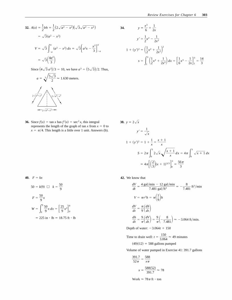
32.
Since we have Thus,
2 a x− 22
2 a x− 22
2 a x− 22
a � 3�5�32
� 1.630 meters.
a3 � �5�3�2.�4�3 a3�3 � 10,
� �3�4a3
3 �
V � �3 �a
�a
�a2 � x2� dx � �3a2x �x3
3 �a
�a
� �3 �a2 � x2�
A�x� �12
bh �12
�2�a2 � x2���3�a2 � x2 � 34.
s � �3
1 �1
2x2 �
12x2� dx � 1
6x3 �
12x�
3
1�
143
1 � �y��2 � �12
x2 �1
2x2�2
y� �12
x2 �1
2x2
y �x3
6�
12x
36. Since has this integral represents the length of the graph of tan x from to
This length is a little over 1 unit. Answers (b).x � �4.x � 0
f��x� � sec2 x,f �x� � tan x
Review Exercises for Chapter 6 303
38.
� 4��23��x � 1�32�
3
0�
56�
3
S � 2� �3
0 2�x�x � 1
x dx � 4� �3
0 �x � 1 dx
1 � �y��2 � 1 �1x
�x � 1
x
y� �1�x
y � 2�x
40.
� 225 in � lb � 18.75 ft � lb
W � �9
0 509
x dx � 259
x2�9
0
F �509
x
50 � k�9� ⇒ k �509
F � kx 42. We know that
Depth of water:
Time to drain well: minutes
Volume of water pumped in Exercise 41: 391.7 gallons
Work � 78� ft � ton
x �588�52�391.7
� 78
391.752�
�588x�
�49��12� � 588 gallons pumped
t �150
3.064� 49
�3.064t � 150
dhdt
�9� �dV
dt � �9� �� 8
7.481� � �3.064 ftmin.
dVdt
��
9 �dhdt �
V � �r2h � ��19�h
dVdt
�4 galmin � 12 galmin
7.481 galft3� �
87.481
ft3min

304 Chapter 6 Applications of Integration
44. (a) Weight of section of cable:
Distance:
(b) Work to move 300 pounds 200 feet vertically:
� 40 ft � ton � 30 ft � ton � 70 ft � ton
Total work � work for drawing up the cable � work of lifting the load
200�300� � 60,000 ft � lb � 30 ft � ton
W � 4 �200
0 �200 � x� dx � �2�200 � x�2�
200
0� 80,000 ft � lb � 40 ft � ton
200 � x
4 x
46.
� 51 ft � lbs � ��9 � 54� � ��96 � 192 � 54 � 144�
� �19
x2 � 6x�9
0� �2
3x2 � 16x�
12
9
W � �9
0 ��2
9x � 6� dx � �12
9 ��4
3x � 16� dx
F�x� � ���29�x � 6,��43�x � 16,
0 ≤ x ≤ 9 9 ≤ x ≤ 12
W � �b
a
F�x� dx
48.
�x, y � � �1, 175 �
�3
649x � 6x2 �43
x3 �15
x5�3
�1�
175
( , )x y
−3 3 6
3
6
9
x
y
�3
64 �3
�1 �9 � 12x � 4x2 � x4� dx y � � 3
32�12
�3
�1 ��2x � 3�2 � x4 dx
�3
3232
x2 �23
x3 �14
x4�3
�1� 1 x �
332
�3
�1 x�2x � 3 � x2� dx �
332
�3
�1 �3x � 2x2 � x3� dx
1A
�3
32
A � �3
�1 ��2x � 3� � x2 dx � x2 � 3x �
13
x3�3
�1�
323
50.
�x, y � � �103
, 4021�
�12 �
516�
37
x73 �1
12x3�
8
0�
4021
y � � 516�
12
�8
0 �x43 �
14
x2� dx
� �516
38
x83 �16
x3�8
0�
103
x �5
16 �8
0 x�x23 �
12
x� dx
1A
�5
16
A � �8
0 �x23 �
12
x� dx � 35
x53 �14
x2�8
0�
165
x
−2
2
2
6
4
4
6 8
( , )x y
y