Part IB Quantum Mechanics, Michaelmas 2019

Tuesday and Thursday, 11.05 a.m. to 11.55 a.m., Mill Lane lecture room 3

Prof. Adrian Kent (apak@damtp.cam.ac.uk)

I am very grateful to previous lecturers of this course, and in particular toJonathan Evans and Eugene Lim, who very generously shared their lecture notesand thoughts on the material. These notes have been influenced by their presenta-tions of many of the course topics, and sometimes draw directly on their discussions.I am also grateful to past students of the course, whose feedback and correctionshave been very helpful. More feedback – whether noting typos or other errors ormore general comments – would be very welcome!

The completed lecture notes are intended to be a reasonably complete summaryof the course. However, material not covered in the printed notes will be addedduring lectures, for instance in answer to questions (which are encouraged!) orwhenever there is time for further discussion that could be helpful. Non-examinablesections of the lecture notes are marked by asterisks at the start and the end. Somefootnotes also contain references to results proved in textbooks or other referencesbut not in the notes: these proofs too are, obviously, non-examinable.

Further course material will be added from time to time on the course web page,which is linked from www.qi.damtp.cam.ac.uk (follow the link to Undergraduate andMasters Lecture Courses on the left menu).

If you wish to make additional notes during lectures you will probably find itsimplest to make them on separate sheets of paper, with footnote numbers to referthem to the appropriate place in the printed notes.

Highlights of this course:

• Historical development of quantum mechanics

• The one-dimensional Schrodinger equation; solution for particles in variouspotentials; probabilistic interpretation; beam scattering and tunneling.

• The basic formalism of quantum mechanics – states, operators, observables,measurement, the uncertainty principle: a new way of treating familiar dy-namical quantities (position, momentum, energy, angular momentum).

• Quantum mechanics in three dimensions: the 3D Schrodinger equation, an-gular momentum, the hydrogen atom and other solutions of the 3D SE.

Version dated 27.08.19. Any updated versions will be placed on the course webpage linked from www.qi.damtp.cam.ac.uk.

1

Recommended books

(*) R. Feynman, R. Leighton and M. Sands, Feynman lectures on physics, volume3, chapters 1-3 (Addison-Wesley, 1989).

A beautifully written and profoundly thoughtful introduction to some of thebasic ideas of quantum theory. Feynman was one of the twentieth century’s mostcreative physicists. As these chapters illustrate, he also thought very deeply andcarefully about fundamental questions in physics and about the scientific processitself. I really recommend these chapters very strongly as background reading forthe course.

(*) A. Rae and J. Napolitano, Quantum Mechanics, chapters 1-5 (IOP Publish-ing, 2002).

A very good textbook which covers a range of elementary and more advancedtopics in quantum theory, including a short discussion of the conceptual problemsof quantum mechanics. The first five chapters form a good course text for IB QM.

(*) S. Gasiorowicz, Quantum Physics (Wiley 2003).A very nicely and clearly written book, with good illustrations, which covers

most of the course material well.

P. Landshoff, A. Metherell and G. Rees, Essential Quantum Physics (CambridgeUniversity Press, 2001).

Another nicely and concisely written textbook, which also covers most of thecourse material for IB QM well.

P. A. M. Dirac, The Principles of Quantum Mechanics (Oxford University Press,1967; reprinted 2003).

A more advanced treatment. Despite its age it is still a valuable exposition ofthe insights and perspectives of one of the pioneers of quantum theory. You maywant to consider looking at this if you intend to go beyond this course and pursuePart II and Part III courses in quantum physics.

S. Brandt and H.D. Dahmen, The Picture Book of Quantum Mechanics (4thedition; Springer, 2012). An excellent book with accompanying plots and simu-lations. These give visual explanations that nicely illuminate the mathematics ofsolutions of the Schrodinger equation, tunnelling, reflection from barriers, atomicelectron states, and other quantum phenomena.

(*) Particularly recommended.

2

Contents

1 Quantum Mechanics, science and technology 51.1 Quantum Mechanics and fundamental science . . . . . . . . . . . . . 51.2 Quantum Mechanics and technology . . . . . . . . . . . . . . . . . . 6

2 Historical development of quantum mechanics 72.1 Planck’s quantum hypothesis (1900) . . . . . . . . . . . . . . . . . . 72.2 Einstein’s explanation of the photoelectric effect (1905) . . . . . . . 82.3 Diffraction of single photons (1909) . . . . . . . . . . . . . . . . . . . 92.4 The Rutherford atom (1911) . . . . . . . . . . . . . . . . . . . . . . 102.5 The Bohr atom (1913) . . . . . . . . . . . . . . . . . . . . . . . . . . 102.6 Compton scattering (1923) . . . . . . . . . . . . . . . . . . . . . . . 142.7 Wave and particle models of electromagnetic radiation . . . . . . . . 152.8 De Broglie waves (1924) . . . . . . . . . . . . . . . . . . . . . . . . . 152.9 Matter wave diffraction (1923-7) . . . . . . . . . . . . . . . . . . . . 162.10 Discussion of the double slit experiment . . . . . . . . . . . . . . . . 16

2.10.1 What can we conclude from double slit experiments? . . . . 192.11 *Ongoing tests of quantum theory . . . . . . . . . . . . . . . . . . . 212.12 Closing comments . . . . . . . . . . . . . . . . . . . . . . . . . . . . 21

3 The one-dimensional Schrodinger equation 233.1 The 1D Schrodinger equation for a free particle . . . . . . . . . . . . 233.2 The momentum operator . . . . . . . . . . . . . . . . . . . . . . . . 243.3 The 1D Schrodinger equation for a particle in a potential . . . . . . 253.4 The wavefunction . . . . . . . . . . . . . . . . . . . . . . . . . . . . . 26

3.4.1 What is the wavefunction? . . . . . . . . . . . . . . . . . . . 263.4.2 What the wavefunction definitely isn’t . . . . . . . . . . . . . 27

3.5 The superposition principle . . . . . . . . . . . . . . . . . . . . . . . 273.6 Probabilistic interpretation of the wavefunction: the Born rule . . . 28

3.6.1 Probability density and probability current . . . . . . . . . . 29

4 Solutions of the 1D Schrodinger equation 314.1 Example I: Stationary states . . . . . . . . . . . . . . . . . . . . . . 314.2 Completeness of the energy eigenfunctions . . . . . . . . . . . . . . . 324.3 Example II: Gaussian wavepackets . . . . . . . . . . . . . . . . . . . 344.4 Example III: Particle in an infinite square potential well . . . . . . . 35

4.4.1 Handling discontinuities . . . . . . . . . . . . . . . . . . . . . 364.5 Parity . . . . . . . . . . . . . . . . . . . . . . . . . . . . . . . . . . . 384.6 Example IV: Particle in a finite square well . . . . . . . . . . . . . . 384.7 Example V: The quantum harmonic oscillator . . . . . . . . . . . . . 41

5 Tunnelling and Scattering 455.1 Scattering states . . . . . . . . . . . . . . . . . . . . . . . . . . . . . 455.2 Interpretation of plane wave scattering solutions . . . . . . . . . . . 465.3 Example I: The potential step . . . . . . . . . . . . . . . . . . . . . . 475.4 Example II: The square potential barrier . . . . . . . . . . . . . . . . 49

5.4.1 *Important examples . . . . . . . . . . . . . . . . . . . . . . . 51

6 The basic formalism of quantum mechanics 526.1 Spaces of functions . . . . . . . . . . . . . . . . . . . . . . . . . . . . 526.2 The inner product . . . . . . . . . . . . . . . . . . . . . . . . . . . . 52

6.2.1 Properties of the inner product . . . . . . . . . . . . . . . . . 526.3 Operators . . . . . . . . . . . . . . . . . . . . . . . . . . . . . . . . . 53

3

6.3.1 Some examples of operators . . . . . . . . . . . . . . . . . . . 536.4 Hermitian operators . . . . . . . . . . . . . . . . . . . . . . . . . . . 53

6.4.1 Classical states and dynamical variables . . . . . . . . . . . . 536.4.2 Quantum states and observables . . . . . . . . . . . . . . . . 54

6.5 Some theorems about hermitian operators . . . . . . . . . . . . . . . 546.6 Quantum measurement postulates . . . . . . . . . . . . . . . . . . . 576.7 Expectation values . . . . . . . . . . . . . . . . . . . . . . . . . . . . 586.8 Commutation relations . . . . . . . . . . . . . . . . . . . . . . . . . . 59

6.8.1 The canonical commutation relations . . . . . . . . . . . . . . 606.9 Heisenberg’s Uncertainty Principle . . . . . . . . . . . . . . . . . . . 61

6.9.1 What does the uncertainty principle tell us? . . . . . . . . . . 636.10 Ehrenfest’s theorem . . . . . . . . . . . . . . . . . . . . . . . . . . . 64

6.10.1 Applications of Ehrenfest’s theorem . . . . . . . . . . . . . . 656.11 *The harmonic oscillator revisited . . . . . . . . . . . . . . . . . . . 65

7 The 3D Schrodinger equation 687.1 Quantum mechanics in three dimensions . . . . . . . . . . . . . . . . 687.2 Spherically symmetric potentials . . . . . . . . . . . . . . . . . . . . 707.3 Examples of spherically symmetric potentials . . . . . . . . . . . . . 72

7.3.1 The spherical harmonic oscillator . . . . . . . . . . . . . . . . 727.3.2 The spherical square well . . . . . . . . . . . . . . . . . . . . 72

7.4 Spherically symmetric bound states of the hydrogen atom . . . . . . 727.5 Canonical Commutation Relations in 3D . . . . . . . . . . . . . . . . 757.6 Orbital Angular Momentum . . . . . . . . . . . . . . . . . . . . . . . 75

7.6.1 Angular momentum commutation relations . . . . . . . . . . 757.6.2 Angular momentum operators in spherical polar coordinates 77

7.7 Solving the 3D Schrodinger equation for a spherically symmetric po-tential . . . . . . . . . . . . . . . . . . . . . . . . . . . . . . . . . . . 797.7.1 Degeneracies . . . . . . . . . . . . . . . . . . . . . . . . . . . 80

7.8 The Hydrogen atom . . . . . . . . . . . . . . . . . . . . . . . . . . . 817.8.1 Energy level degeneracies . . . . . . . . . . . . . . . . . . . . 82

7.9 Towards the periodic table . . . . . . . . . . . . . . . . . . . . . . . . 83

4

1 Quantum Mechanics, science and technology

1.1 Quantum Mechanics and fundamental science

Quantum mechanics is the non-relativistic version of relativistic quantum field the-ory. Collectively, we refer to these theories as “quantum theory”. Most physicistswould agree quantum theory is the most remarkable, interesting and surprisingphysical theory we have discovered.1 Although ultimately only a non-relativisticpart of a larger theory, quantum mechanics already teaches us that our universefollows laws that involve beautiful and intricate mathematics, and whose form wecould not possibly have imagined had they not been illuminated by experiment.

Among other things, quantum mechanics explains the essential features of thefollowing:

• the structure of atoms and molecules and their chemical interactions; i.e.chemistry, and biochemistry and so, in principle, biology. We will begin todiscuss this towards the end of the course, when we consider quantum mechan-ical descriptions of the hydrogen atom and, more qualitatively, other atoms.This description is made more precise and taken further in Part II Principlesof Quantum Mechanics.

• the structure and properties of solids (and so, in principle, much of classicalmechanics). Conductivity (some basic theory of which is introduced in PartII Applications of Quantum Mechanics) and superconductivity.

• the thermodynamics of light and other electromagnetic radiation and also howelectromagnetic radiation interacts with matter. To describe this properlyrequires relativistic quantum field theory, which isn’t covered until Part III.

• the physics of subatomic particles, radioactivity, nuclear fission and fusion.Again, we need relativistic quantum field theory to describe these phenomenain full detail. But, as we’ll see later, even elementary quantum mechanicsgives us some useful insights into the physics of nuclear fission and fusion. Forexample, we can understand the random nature of these processes, and theway fusion and fission rates depend on relevant potentials, as a consequenceof quantum tunnelling.

Modern cosmological models are also based on quantum theory. Since we do nothave a quantum theory of gravity, and do not know for sure whether there is one,these cosmological models are at best incomplete. Nonetheless they give a goodqualitative fit to observational data. Many physicists hope that this project can becompleted, so that we can describe the entire universe and its evolution by quantumtheory.2 These topics are covered in detail in the Part II and Part III Cosmologycourses.

1Einstein’s general theory of relativity is the only other contender. It is an extraordinarilybeautiful theory that transformed our understanding of space and time and their relationship tomatter, and that gave us the tools to understand the cosmos. The two theories are fundamentallyincompatible, and it is uncertain precisely which parts of which theory will survive in a future uni-fication. Still, I find quantum theory more intriguing, because of the variety of deep mathematicalconcepts it combines and because it is so different from and so much stranger than the theoriesthat preceded it.

2It is also true that many thoughtful physicists suspect that the project cannot be completed,because we will need something other than a quantum theory of gravity, or because quantumtheory will turn out not to hold on large scales. If so, comparing quantum cosmological models toobservation should eventually give us insight into new physics.

5

1.2 Quantum Mechanics and technology

Many of the revolutionary technological developments of the last hundred years relyon quantum mechanics:

• semiconductor physics – transistors, diodes, integrated circuits, and hence thecomputing and IT industries.

• laser physics

• nuclear power and the as yet unrealised dream of controllable fusion power

• tunnelling electron microscopy and atomic manipulation

• More recent inventions relying on the distinctive properties of quantum infor-mation. These include quantum cryptography. Its best known application isquantum key distribution, which in principle allows perfectly secure commu-nication, and is now practical with large data transmission rates and over longdistances, including between satellite and ground stations. There are manyother applications, including quantum authentication, quantum position ver-ification, quantum bit string commitment, quantum multi-party computationand quantum digital signatures. Quantum information allows perfect securityfor some of these tasks, and security advantages for others.

Another major development has been the invention of quantum algorithmsand various types of quantum computers. We now know that quantum com-puters are substantially more efficient than classical computers for some im-portant applications, including factorisation (at least compared to the bestknown classical algorithms) and the simulation of quantum systems. Smallscale quantum computers have been built, and many research groups are com-peting to build a quantum computer large enough to exploit the theoreticaladvantages. In September 2019, Google claimed the first demonstration ofso-called “quantum supremacy”, a calculation on a quantum computer thatis infeasible on classical computers.3

Other fascinating applications include quantum teleportation – which in prin-ciple gives a way of effectively deleting a physical system at A and recreatingit at B without sending it along a path from A to B – and other types ofquantum communication.

All of these topics are covered in the Part II Quantum Information and Com-putation course. Notes for that course, and for Part III courses in this area,along with some information about research work on these topics in DAMTP,can be found on http://www.qi.damtp.cam.ac.uk.

3There are nuances of definition here, and the community is still assessing the claim.

6

Figure 1: Google’s Bristlecone quantum processor. Image on left, map of qubitconnections on right.

2 Historical development of quantum mechanics

2.1 Planck’s quantum hypothesis (1900)

One of the great puzzles in late 19th century physics was the inability of clas-sical thermodynamics and electromagnetism to predict the correct spectrum — orindeed any sensible spectrum — for the frequency distribution of radiation froman idealized black body. Classical thermodynamics predicted an emission spectrumwhich suggested that the flux of emitted radiation tends to infinity as the frequencytends to infinity, and hence that an infinite amount of energy is emitted per unittime. In 1900, Max Planck showed that one could predict the experimentally ob-served spectrum by postulating that, because of some (at that point) unknownphysics, matter can emit or absorb light of frequency ν only in discrete quantawhich have energy

E = hν = �ω . (2.1)

Here ω = 2πν is the light’s angular frequency (the numberof radians of oscillation per second), and

� =h

2π≈ 1.055× 10−34 Joule sec . (2.2)

The constant h is a new constant of nature (Planck’s constant). For most purposesit turns out to be notationally more convenient to use � rather than h, and we willgenerally do so.

7

2.2 Einstein’s explanation of the photoelectric effect (1905)

Experiment shows that light hitting a metal surface in a vacuum can causeelectrons to be ejected with a range of energies. To emit any electrons, the incidentlight needs to have angular frequency ω satisfying ω ≥ ωmin, where ωmin is a constantdepending on the particular metal. When ω ≥ ωmin, one finds that the maximumenergy of the emitted electrons, Emax, obeys

Emax = �ω − �ωmin ≡ �ω − φ , (2.3)

where φ is the so-called work function of the metal. The average rate of electronemission is found to be proportional to the intensity of the incident light, butindividual electrons appear to be emitted at random (and so in particular, measuredover small enough time intervals, the emission rate fluctuates).

𝑒−𝑒−𝑒− 𝑒−𝑒−

𝑒− 𝑒−

𝑒−𝑒−

Incoming light Emitted electrons

Figure 2: Schematic illustration of the photoelectric effect.

Although light had been understood as an electromagnetic wave, it was hard toexplain these effects in terms of a wave model of light. If we think of an incidentwave transmitting energy to the electrons and knocking them out of the metal, wewould expect the rate of electron emission to be constant (i.e. we would not expectrandom fluctuations), and we would also expect that light of any frequency wouldeventually transmit enough energy to electrons to cause some of them to be emitted.

To explain the photoelectric effect, Albert Einstein (in 1905) was led to postulateinstead that light is quantised in small packets called photons, and that a photon ofangular frequency ω has energy �ω. He reasoned that two photons are very unlikelyto hit the same electron in a short enough time interval that their combined effectwould knock the electron out of the metal: the energy an electron acquires frombeing hit by a photon is very likely to have dissipated by the time it is hit again.

8

Thus, one can explain the photoelectric effect as the result of single photons hittingelectrons near the metal surface, if one assumes that an electron needs to acquirekinetic energy ≥ φ to overcome the binding energy of the metal. An electron whichacquires energy �ω thus carries away energy ≤ �ω−φ = Emax. One can also explainthe emission rate observations: the average rate of photon arrival is proportionalto the intensity of the light, and the rate of emission of electrons is proportionalto the rate of photon arrival. However, individual photons arrive, and hit electronsso as to knock them out of the metal, at random – hence the randomly distributedemissions of electrons.

2.3 Diffraction of single photons (1909)

In Cambridge in 1909, J.J. Thomson suggested to G.I. Taylor (who had asked fora research project) that he investigate the interference of light waves of very lowintensity. Taylor carried out an experiment in which a light source was successivelyfiltered so that the energy flux was equivalent to the flux of a source sending nomore than one photon at a time through the apparatus. He then observed thephotographic image built up by diffraction of this feeble light around a needle. Thecharacteristic diffraction pattern – the same pattern seen for strong light sources –was still observed.

Figure 3: Photograph of diffraction bands caused by a thin wire in feeble light.See: Taylor, Proc. Camb. Phil. Soc., 15, 114, 1909. The exposure was 400 hours.Source: Cavendish Laboratory. Licensed under Creative Commons.

This seems to suggest that single photons propagate through the apparatus andnonetheless “self-interfere” in such a way that the diffraction pattern is cumulativelybuilt up. This is indeed how Taylor’s results were interpreted for several decadesafter the development of quantum mechanics in 1926. Problems were later noticed

9

with this interpretation of this particular experiment: having the average energy fluxof a single photon does not always imply that a source is emitting single photons.However, the experiment was subsequently repeated with genuine single photonsources, still showing the same diffraction pattern. Qualitatively similar patternsare seen in diffraction experiments for single electrons and other types of matter(see below).

2.4 The Rutherford atom (1911)

After discovering the electron in 1897, J.J. Thomson proposed a model of theatom as a sort of “plum pudding” with Z pointlike electrons of charge −e embeddedin a sphere of positive charge +Ze.

Geiger and Marsden’s famous experiment, carried out at Rutherford’s sugges-tion, tested for large angle scattering of a beam of α-particles directed at gold foil.One would not expect significant scattering from a loosely distributed low chargedensity “plum pudding” atom, and Rutherford thought it unlikely anything interest-ing would be observed. But, in fact, some α-particles were observed to be scatteredthrough angles of up to 180◦. In Rutherford’s famous phrase,

“It was as if you fired a 15-inch shell at tissue paper and it cameback and hit you.”

The scattering suggests a high density positive charge within the atom. Rutherfordthus postulated a new model of the atom, with a heavy nearly pointlike nucleus, ofcharge +Ze, surrounded by Z electrons in orbit.

(A short popular account can be found athttp://physicsopenlab.org/2017/04/11/the-rutherford-geiger-marsden-experiment/.)

2.5 The Bohr atom (1913)

Although the Rutherford atom was more compatible with the Geiger-Marsdenscattering data than was the “plum pudding” model, it had a number of theoreticaldefects.

First, according to Maxwell’s electrodynamics, electrons in orbit around a nu-cleus would radiate, since they are continually undergoing acceleration. This wouldcause them to lose energy and fall in towards the nucleus. Stationary electronswould also fall into the nucleus because of electrostatic attraction. This wouldsuggest that atoms must be unstable, which they generally are not.

Second, the model fails to explain why atoms have characteristic line spectra cor-responding to discrete frequencies at which they absorb or emit light. For example,hydrogen has frequencies given by the Rydberg formula (Rydberg, 1890):

ωmn = 2πcR0(1

n2− 1

m2) for m > n , (2.4)

where the Rydberg constant

R0 ≈ 1.097× 107 m−1 . (2.5)

Third, it fails to explain why atoms belong to a finite number of chemical species,with all members of the same species behaving identically. For instance, if a hydro-gen atom can have an electron in any type of orbit around its nucleus, one wouldexpect infinitely many different types of hydrogen atom, corresponding to the in-finitely many different possible orbits, and one would expect the atoms to havedifferent physical and chemical properties, depending on the details of the orbit.

10

Figure 4: Schematic illustration of the Geiger-Marsden experiment, from the webpage cited above.

Niels Bohr, in 1913, observed that these problems could be resolved in a wayconsistent with Planck’s and Einstein’s earlier postulates, if we suppose that theelectron orbits of hydrogen atoms are quantised so that the orbital angular momen-tum takes one of a discrete set of values

L = n� , (2.6)

where n is a positive integer.

Thus, if we take an electron e moving with velocity v in a circular orbit of radius

r about a proton p, F = mea gives us that the Coulomb force

e2

4π�0r2=

mev2

r. (2.7)

If we also have

L = mevr = n� (2.8)

then

n2�2

r3me=

e2

4π�0r2(2.9)

and hence

r = n2(�24π�0mee2

) = n2a0 , (2.10)

11

Figure 5: Spectra for the hydrogen atom. The figure shows three horizontal linesat small distances from each other. Between the two lower lines, the Lyman series,with four vertical red bands in compact form, is shown. This has nf = 1 and ni ≥ 2,and wavelengths in the range 91− 100 nanometers. The Balmer series is shown tothe right side of this series. This has nf = 2 and ni ≥ 3, and wavelengths in therange 365 − 656 nanometers. At the right side of this, the Paschen series bandsare shown. This has nf = 3 and ni ≥ 4, and wavelengths in the range 820 − 1875nanometers. The Rydberg formula is obtained by taking nf = n, ni = m.Source for figure and caption: https://opentextbc.ca/physicstestbook2Image licenced under Creative Commons.

where

a0 =4π�0�2

mee2≈ 0.53× 10−10 m (2.11)

is the Bohr radius.We can then obtain the energy of the n-th Bohr orbit from (2.7) and the Coulomb

potential:

En =1

2mev

2− e2

4π�0r= − e2

8π�0r= − e2

8π�0n2a0= − e4me

32π2�20�21

n2=

E1

n2,

(2.12)where

E1 = − e4me

32π2�20�2≈ −13.6 eV . (2.13)

Thus we have n = 1 with energy E = E1 defining the lowest possible energystate, or ground state, of the Bohr atom. The higher energy excited states, so calledbecause they can be created by “exciting” the ground state atom with radiation,correspond to n > 1. These can decay to the ground state: the ground state has nolower energy state to decay to, and so is stable. (The Bohr model does not allow astate with zero orbital angular momentum, which would correspond to n = 0, r = 0and E = −∞.)

12

The energy emitted for a transition from the m-th to the n-th Bohr orbital isEmn = Em − En. Using Emn = �ωmn, where ωmn is the angular frequency of theemitted photon, we have

ωmn = 2πR0c(1

n2− 1

m2) , (2.14)

where

R0 =mec

2�(

e2

4π�0�c)2 , (2.15)

which agrees well with the experimentally determined value of the Rydberg con-stant.

Figure 6: The orbits of Bohr’s planetary model of an atom; five concentric circlesare shown. The radii of the circles increase from innermost to outermost circles.On the circles, labels E1, E2, up to Ei are marked. Source for figure and caption:https://opentextbc.ca/physicstestbook2Licenced under Creative Commons.

Bohr’s model of the atom was rather more successful than its predecessors. Itpredicts the energy levels of the hydrogen atom and the spectrum of photons emittedand absorbed. It also accounted for spectroscopic data for ionised helium (He+) andfor some emission and absorption spectra for other atoms. (We now understand thatthese are the spectra produced by the innermost electrons, which can be modelledin a way qualitatively similar to the electron in the hydrogen atom.)

However, as Bohr himself stressed, the model offered no explanation of atomicphysics. For example, as Rutherford commented, it’s quite mysterious that anelectron which jumps from them-th to the n-th orbit seems to know in advance whatfrequency to radiate at during the transition. Moreover, the Bohr model is quite

13

wrong about the details of electron orbits, even for the hydrogen atom. Nonetheless,it was an important stepping stone on the path to quantum mechanics, suggestingsome link between Planck’s constant, atomic spectra and atomic structure, and thequantisation of angular momentum and other dynamical quantities.

2.6 Compton scattering (1923)

In 1923, Arthur Holly Compton observed the scattering of X-rays by electronsassociated with atoms in a crystal. Because the X-ray energies were much largerthan the electron binding energies, the electrons can effectively be modelled byfree electrons. Indeed, we also directly observe that if an electron beam and anX-ray beam converge, some electrons and some X-rays are deflected. This is verydifficult to reconcile with a pure wave model of electromagnetic radiation, becausethe energy and momentum transfer for individual scatterings does not depend onthe intensity of the X-ray beam.

A simple alternative explanation is that the scattering results from collisionsbetween a single photon in one beam and a single electron in the other, in whichenergy and momentum are transferred between the photon and the electron. (Arelativistic treatment of this scattering process was given in the IA Dynamics andRelativity course.) This explanation is consistent with the observed scattering dataand with conservation of (relativistic) energy and momentum, provided we assumethat a photon of angular frequency ω has a definite momentum

p = �k , (2.16)

where k is the wave vector of the corresponding electromagnetic wave, so that

|p| = �ωc

= �|k| . (2.17)

14

2.7 Wave and particle models of electromagnetic radiation

We thus see the emergence of two different models of light and other electro-magnetic radiation.

Sometimes (classical electromagnetism, diffraction experiments with a stronglight source, . . .) it is useful to model light in terms of waves:

ei(k.x−ωt) , (2.18)

where k is the wave vector, ω the angular frequency, c = ω|k| the speed of light in a

vacuum, and the wavelength λ = 2πcω = 2π

|k| .

Sometimes (photoelectric effect, spectroscopy in the Bohr model of the hydrogenatom, Compton scattering, . . .) it is useful to adopt a particle model, in which lightis made up of photons with energy and momentum

E = �ω , p = �k . (2.19)

The word “model” is chosen deliberately here. A model can be useful (as thewave and particle models of light are, in the appropriate contexts) without be-ing completely correct. Indeed, G.I. Taylor’s 1909 demonstration of single photondiffraction already gave an example of a single experiment for which neither thewave nor the particle model of light appeared to be adequate. A simple particlemodel would not predict the observed diffraction pattern, while a simple wave modelcannot explain the observation of single photons recorded on the photographic film.4

2.8 De Broglie waves (1924)

Louis de Broglie reexamined and extended Einstein’s photon hypothesis. If,he argued, Einstein was right that light waves can be considered as composed ofparticles – photons – might it not equally be the case that objects like electrons,which were thought of as particles, could exhibit wave-like behaviour?

As he pointed out in his 1924 PhD thesis, this would make the Bohr angularmomentum quantization condition

L = pr = n� (2.20)

at least somewhat less mysterious. If we suppose that an electron of momentum pcan (somehow) be thought of as a wave with de Broglie wavelength

λ =2π�p

, (2.21)

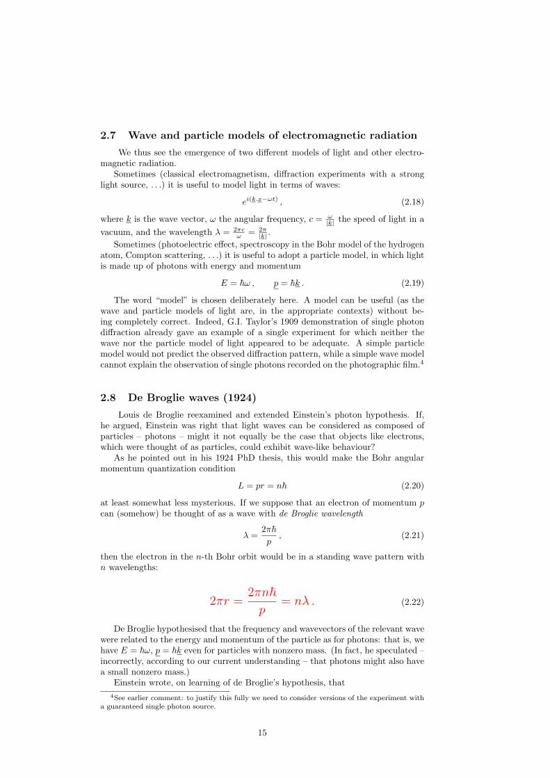
then the electron in the n-th Bohr orbit would be in a standing wave pattern withn wavelengths:

2πr =2πn�p

= nλ . (2.22)

De Broglie hypothesised that the frequency and wavevectors of the relevant wavewere related to the energy and momentum of the particle as for photons: that is, wehave E = �ω, p = �k even for particles with nonzero mass. (In fact, he speculated –incorrectly, according to our current understanding – that photons might also havea small nonzero mass.)

Einstein wrote, on learning of de Broglie’s hypothesis, that

4See earlier comment: to justify this fully we need to consider versions of the experiment witha guaranteed single photon source.

15

De Broglie’s model of the atom. Electrons occupy orbits corresponding to a integer multiple of their de Broglie wavelength.

Figure 7: Schematic illustration of the de Broglie model of electron orbits in anatom.

“I believe it is the first feeble ray of light on this worst of our physicsenigmas.”

It was.

2.9 Matter wave diffraction (1923-7)

We know that the wave model of light predicts, correctly, that light should forminterference and diffraction patterns. De Broglie’s hypothesis suggests the sameshould be true of electrons and other massive particles. This was first confirmed inexperiments carried out (from 1923-7) by Davisson and Germer and (independentlyin 1927) by G.P. Thomson, who observed diffractive scattering of electrons frommetallic crystals, with diffraction patterns consistent with the de Broglie wavelengthλ = 2π�

p .G.P. Thomson was the son of J.J. Thomson, who in 1897 discovered the electron,

in experiments in which it behaves as (and so was then understood to be) a particle.It is a pleasing historical quirk that G.P. Thomson was the co-discoverer of thewave-like behaviour of electrons in diffraction experiments.

Many diffraction experiments with electrons, neutrons and other particles havesince been carried out, all confirming de Broglie’s prediction.

2.10 Discussion of the double slit experiment

(Cf Feynman volume III chapters I-III)A nice version of the double slit experiment with electrons was carried out by

Akira Tonomura. It is described athttp://www.hitachi.com/rd/portal/highlight/quantum/doubleslit/index.html

Like the other diffraction experiments mentioned above, this shows that electronsand other massive particles can produce interference patterns in the same sort ofway as light and water waves. At the same time, it gives very vivid evidence ofelectrons being detected as individual particles. We stress again that both the wavedescription and the particle description are just models that are sometimes usefulbut, as this experiment again illustrates, not fundamentally correct. To analyse this

16

Figure 8: Single electron detection events building up an interference pattern inTonomura’s experiment. Copyright in these documents published on Hitachi World-Wide Web Server is owned by Hitachi, Ltd.

conclusion in more detail, let’s follow Feynman in considering an idealised versionof the double slit experiment, in which we assume we have perfect detectors thatcan register the passage of an electron without affecting it.

The observed interference pattern in a double slit experiment agrees with thatpredicted by a wave model (and disagrees with that predicted by a particle model).But the electrons arrive individually at the detector, which registers each time onearrives — as a particle model (but not a wave model) would suggest. The same istrue of other massive particles, and also of photons. Even if we reduce the intensityof the source so that only one electron on average is between the source and thescreen at any given time, we still see individual electrons detected in a pattern thatcumulatively reproduces the distribution predicted by the wave model.

It’s tempting to think that, when electrons leave the source, they behave likebullets from a gun – i.e. like particles coming from a well-defined small region.Certainly if we place a detector near the source this is what the detections suggest(although if we do this the electrons don’t continue into the rest of the apparatus).It’s also tempting to think that, since the electrons (etc.) arrive at the detector andare detected there as particles, with a definite or nearly definite position, they musthave behaved like classical particles throughout, following some definite path fromthe source, through one hole or the other, to the detector. But, tempting thoughthis last intuition may be, it’s hard to reconcile with the observed interferencepattern. If the electrons behaved like bullets throughout, we’d expect somethinglike a superposition of two Gaussian distributions from the two slits, instead of thepattern of minima and maxima we observe.

17

Quantum weirdness: the double slit experiment

The observed patterns for one and two slits fitvery well with a wave model of light, and seem to refute a model in which light is made up of particles.

Figure 9: The double slit experiment.

There seems, in any case, a simple way to investigate more closely. Supposethat we have ideal detectors, which register that an electron has passed through aregion, but don’t obstruct its path. We can set up a double slit experiment withone of these ideal detectors adjacent to each slit (for definiteness, let us say they areon the far side, between the slit and the screen). Now we don’t need to speculate:we can observe which slit the electron goes through. But when we do this, theinterference pattern changes: we see a superposition of two Gaussians, as predictedby a particle model, rather than the pattern of maxima and minima predicted bythe wave model and observed in the previous experiment.

18

What is really going on in the double slit experiment? 

Light source

ScreenAbsorbing filterwith two slits

Why not just look and see which slit the photon goes through?

What if we include passive detectors registering which slit the photon goes through?

By introducing new detectors, we changedthe experiment.

Quantum theory predicts, and experimentconfirms, that this changes the outcome.

Figure 10: Observing which slit the electron goes through in the double slit exper-iment.

2.10.1 What can we conclude from double slit experiments?

1. As we already stressed, the wave model and the particle model are just that —models. Neither of them is adequate to explain the behaviour of electrons, photons,or other objects. Each of them can sometimes give a partial explanation of ourobservations, but that explanation is not consistent with all the data.

2. In particular, the type of reasoning about electron paths that would applywithin a particle model does not generally apply in Nature. We can’t assume thatthe electron follows a definite path through one slit or the other, and we can’tassume (as we could with a classical particle) that observing which slit it goesthrough makes no difference to the interference pattern.

3. Some textbooks summarize the state of affairs described in point 1 by sayingthat electrons (photons, etc.) exhibit something called “wave-particle duality”.This term can mislead, if it is interpreted as a sort of explanation of what is goingon rather than just a catchy name for it.

The fact is that our classical wave and particle models are fundamentally inad-equate descriptions. It isn’t correct to say that an electron (or photon, etc.) is botha wave and a particle in the classical senses of either of those words. The electronis something different again, though it has some features in common with both. Togo further, we need a new physical model: quantum mechanics.

4. We saw that the electron interference pattern builds up over time, yet thepoints at which individual electrons hit the screen do not appear to be preciselypredictable: they seem to arrive at random. It might seem natural to speculatethat this apparent randomness might be explained by the fact that we don’t havecomplete data about the experiment. Perhaps, for example, the electrons leave the

19

source in slightly different directions, or perhaps they have some sort of internalstructure that we haven’t yet discussed (and perhaps hasn’t yet been discovered),and perhaps this determines precisely where they hit the screen.

As we’ll see, according to quantum mechanics this is not the case. Quantummechanics, unlike classical mechanics, is an intrinsically probabilistic theory, and ittells us that there is simply no way to predict precisely where the electron will hitthe screen, even if we have a precise and complete description of its physical statewhen it leaves the source.

Now, of course, quantum mechanics might not be the final theory of nature.It’s possible that some as yet unknown and more complete theory could underliequantum mechanics, and it’s logically possible that this theory (if there is one)could be deterministic. However, there are very strong reasons to doubt that anytheory underlying quantum mechanics can be deterministic. In particular, it can beproved (given a few very natural assumptions) that any such theory would be incon-sistent with special relativity. This follows from Bell’s theorem and experimentaltests thereof: it is discussed further in the Part II course “Principles of QuantumMechanics” and in Part III courses.)

20

2.11 *Ongoing tests of quantum theory

Although later developments are beyond the scope of this course, it would bewrong to leave the impression that the historical development of quantum mechan-ics ended in the first part of last century. Indeed, the basic principles of quantummechanics are still being questioned and tested by some theorists and experimen-talists today. Quantum theory is very well confirmed as a theory of microscopicphysics. However, the case for believing that it applies universally to physics on allscales is much weaker.

There is a good scientific motivation for testing any scientific theory in newdomains, which is that theories developed to explain phenomena in one domain maynot necessarily apply in other domains. For example, quantum theory itself showsus the limits of validity of Newtonian mechanics and of classical electrodynamics.Similarly, Einstein’s general theory of relativity shows us the limits of validity ofNewton’s theory of gravity.

There is also a specific motivation for wanting to test quantum theory for macro-scopic systems. This is that the problems in making sense of quantum theory asan explanation of natural phenomena seem to stem from the fact that the classicalphysics we see on macroscopic scales appears to emerge from quantum theory in away that, despite many attempts, remains hard to pin down. Many theorists be-lieve it remains fundamentally unexplained. Many others believe it is explained orexplainable, but there is no real consensus among them about the right explanation.

Interestingly, we know there are consistent (non-relativistic) theories that agreevery precisely with quantum mechanical predictions for microscopic (small mass)particles, but disagree for macroscopic (large mass) ones.

In the past few years, experimental technology has advanced far enough todemonstrate diffraction of quite complex molecules. (Some descriptions of theseexperiments can be found athttps://vcq.quantum.at/; see in particular the work of the Arndt and Aspelmayerresearch groups.) Attempts continue to demonstrate interferometry for larger andlarger objects, motivated not only by the technological challenge but also by thepossibility of testing the validity of quantum mechanics in new domains. In Octo-ber 2019, Fein et al. reported interference experiments for molecules of weightlarger than 25kDa (See https://www.nature.com/articles/s41567-019-0663-9 andthe rather amusing Q and A summaryhttps://www.quantumnano.at/detailview-news/news/facts-fiction-in-reports-on-high-mass-interference/ ).

It should be stressed that there is to date (October 2019) no experimental evi-dence for any deviation from quantum mechanics, which has been confirmed in animpressive array of experiments investigating many different physical regimes. *

2.12 Closing comments

1. As we’ve seen, the photon hypothesis played a key role in the development ofquantum mechanics. We’ve also seen that photons (which are massless) and massiveparticles (such as electrons) produce qualitatively similar interference and diffractionpatterns. However, we won’t have much more to say about photons in this course. Itturns out that we can develop quantum mechanics for the electron and other massiveparticles using relatively simple equations. We can build up a good intuition abouthow quantum systems behave in experiments and in nature from these equations. Afully satisfactory quantum treatment of photons or other massless particles requiresa relativistic quantum theory of fields, which requires more sophisticated concepts(and is much harder to make mathematically rigorous). Quantum electrodynamics,which is a relativistic quantum field theory incorporating photons, is discussed in

21

Figure 11: Interference of molecules larger than 25KDa, from the Fein et al. papercited above.

Part III theoretical physics courses, along with other relevant quantum field theories.2. Although we’ve already seen the classical particle model is inadequate, we

still need some collective name for electrons, protons, neutrons and so on. Perhapsphysicists should have invented another term, but we still call these “particles”. Wewill follow this tradition, so that we might say that the electron is an elementaryparticle, talk about quantum mechanics applied to an abstract particle of mass m,and so forth — always keeping in mind that the classical particle model does notactually apply.

22

3 The one-dimensional Schrodinger equation

3.1 The 1D Schrodinger equation for a free particle

We are first going to develop quantum mechanics in one space (and one time)dimension. We can solve the equations for simple physical models more easily in1D than in 3D and, happily, it turns out that 1D solutions give a good qualitativefeel for a range of interesting 3D physical phenomena.

In 1924, Schrodinger developed de Broglie’s ideas further, into what became astandard way of framing the laws of quantum mechanics.5

Recall that de Broglie postulated that matter is described by waves, and thatthe energy and momentum are related to the angular frequency and wave vector byE = �ω and p = �k, or in one dimension p = �k. We can express this by associatingto a particle of energy E and momentum p a wave of the form

ψ(x, t) = exp(i(kx− ωt)) . (3.1)

Now, for a mass m particle, we have E = 12mv2 = p2

2m , and so

ψ(x, t) = exp(i(kx− ωt)) = exp(i

�(px− p2

2mt)) . (3.2)

Notice that we have taken ψ(x, t) to be complex. Using complex numbers torepresent waves is familiar in classical electromagnetism, where it allows us to com-bine the electric and magnetic fields in a single equation. In that context, it’smathematically convenient, but the real and imaginary parts each have a simplephysical interpretation. We will see that complex-valued solutions to (generalised)wave equations play a more essential role in quantum mechanics.

The simplest wave equation to which the de Broglie wave is the general solutionis the time-dependent 1D Schrodinger equation for a free particle:

1

2m(−i�

∂

∂x)2ψ(x, t) = i�

∂

∂tψ(x, t) . (3.3)

(By a free particle we mean a particle not subject to external forces, i.e. one movingin a potential V (x) = 0.)

5There is an equivalent alternative way of describing quantum mechanics, developed by Heisen-berg, Born and Jordan. But Schrodinger’s formulation is easier to work with and gives a moreintuitive physical picture – so we will follow his approach. Note that “more intuitive” here is arelative statement. As we will see, many of the predictions of quantum mechanics are counter-intuitive. Also, some of the intuitions Schrodinger’s picture suggests may be helpful to us in somecontexts but are not fundamentally justifiable.

23

3.2 The momentum operator

We define the momentum operator

p = −i�∂

∂x. (3.4)

So, for the de Broglie wave ψ(x, t) = exp( i� (px−

p2

2m t)), we have pψ = pψ. In otherwords, acting with the momentum operator on the de Broglie wave is equivalent tomultiplying by the wave momentum.6 We can rewrite (3.3) as

1

2mp2ψ = i�

∂ψ

∂t. (3.5)

This is our first example of a general feature of quantum mechanics. Physicallysignificant quantities (in this case momentum) are represented by operators. Theseoperators act on functions that represent physical states (in this case the idealizedstate defining the de Broglie wave).

Formally, we define an operator O to be a linear map from a space of functions7

to itself, i.e. any map such that

O(a1ψ1 + a2ψ2) = a1Oψ1 + a2Oψ2 (3.6)

for all complex numbers a1, a2 and all functions ψ1,ψ2 in the relevant space.

6This tells us that the de Broglie wave is an eigenfunction of the momentum operator witheigenvalue p: we will define these terms more generally later.

7We will not be too precise about which space of functions we are working with, but willassume that they are suitably “well behaved”. For example, and depending on the context, wemight want to consider the space of infinitely differentiable functions, C∞(R), or the space of“square integrable” functions, i.e. those satisfying Eqn. (3.11).

24

3.3 The 1D Schrodinger equation for a particle in a potential

We want to consider particles subject to a potential V (x) as well as free particles.Examples: alpha rays scattering from a nucleus, electrons diffracting from a

crystal, buckyballs going through an interferometer, neutrons or larger massiveparticles moving in a gravitational field.

To do this, we replace the kinetic energy term in (3.5) by an operator corre-sponding to the hamiltonian or total energy:

H =p2

2m+ V (x) , (3.7)

namely

H =p2

2m+ V (x) , (3.8)

where the second operator corresponds to multiplication by V (x).

This gives the general form of the time-dependent 1D Schrodinger equation fora single particle:

Hψ(x, t) = i�∂ψ

∂t. (3.9)

Or, more explicitly:

− �2

2m

∂2ψ

∂x2+ V (x)ψ = i�

∂ψ

∂t. (3.10)

Note that there is no way to prove mathematically that Eqns. (3.9, 3.10) arephysically relevant, although we have given some motivation for them in the lightof previous physical models and experimental results. As with any new physicaltheory, the only real test is experiment. Since it is not yet obvious what the complex-valued solutions to (3.9, 3.10) have to do with experimentally observable quantities,we will first need to give rules for interpreting them physically, and then test thesepredictions.

25

3.4 The wavefunction

We call a complex valued function ψ(x, t) that is a solution to (3.9) or (3.10) awavefunction. We say the wavefunction ψ(x, t) is normalisable (at time t) if

0 <

� ∞

−∞|ψ(x, t)|2dx < ∞ . (3.11)

Note that for any complex valued ψ(x, t) the integral is real and non-negative.

We say ψ(x, t) is normalised if

� ∞

−∞|ψ(x, t)|2dx = 1 . (3.12)

So, given a normalisable ψ(x, t) with�∞−∞ |ψ(x, t)|2dx = C, so that 0 < C < ∞,

we can define a normalised wavefunction C−1/2ψ(x, t).

3.4.1 What is the wavefunction?

As we will explain in following lectures, the wavefunction ψ(x, t) of a particle isa mathematical object that allows us to calculate the probability of detecting theparticle at any given position if we set up a detector there. More generally, itallows us to calculate the probability of any given outcome for the measurement ofany observable quantity (for example, energy or momentum) associated with theparticle.

Sometimes in the course of your studies you may suspect that lecturers aretemporarily keeping the full truth from you.8 Sometimes you would be right, butnot here. We really don’t have a better and more intuitively comprehensible storyabout the wavefunction.9

8If charitable, you may also suspect there may be good pedagogical reasons for this.9At least, not one that is generally agreed.

26

3.4.2 What the wavefunction definitely isn’t

Schrodinger initially hoped to interpret the wave function as describing a dispersedcloud of physical material that somehow corresponds to a “smeared-out” particle.This looks a natural interpretation at first sight, but proved untenable and wasabandoned.

One problem with this interpretation is that if a charged particle is really adispersed cloud of charge, we would expect to be able to detect bits of the cloudcarrying fractions of the charge of the electron. However, we always find thatcharged objects carry a charge that is some integer multiple of the electron charge.Classical electrodynamics also suggests that a dispersed charge of cloud should in-teract repulsively with itself via the Coulomb force, and thus tend to be additionallydispersed, in a way that we do not observe.

Even if these objections could somehow be overcome, another problem remains.No matter how widely the electron’s wavefunction is spread out in space, when welook for it by setting up detectors we always find an apparently pointlike particlein a definite location. If the wavefunction really represented a dispersed cloud, thiscloud would have to suddenly coalesce into a particle at a single point when wecarry out a measurement. This would mean that parts of the cloud would have totravel extremely fast — often much faster than light speed. This is inconsistentwith special relativity.

3.5 The superposition principle

Exercises 1. The Schrodinger equation

− �2

2m

∂2

∂x2ψ(x, t) + V (x)ψ(x, t) = i�

∂

∂tψ(x, t)

is linear in ψ(x, t): if ψ1 and ψ2 are solutions then a1ψ1+a2ψ2 is a solution too,for any complex a1, a2.

2. If ψ1 and ψ2 are normalisable and a1ψ1 + a2ψ2 is nonzero 10, then it is alsonormalisable.

3. Show that it is not generally true that if ψ1 and ψ2 are normalised thena1ψ1 + a2ψ2 is, even if |a1|2 + |a2|2 = 1.

The linearity of the Schrodinger equation implies the so-called superpositionprinciple: there is a physical solution corresponding to any linear combination oftwo (or more) physical solutions.

The superposition principle is an essential feature of quantum mechanics, whichdoes not generally apply in classical physics. It makes no sense in Newtonianmechanics to add a linear combination of two orbits of a planet around the Sun:this doesn’t define another possible orbit. But in quantum theory, taking sums ofphysical wavefunctions, for example those of an electron orbiting the nucleus of ahydrogen atom, gives us another wavefunction that has a direct physical meaning.

We will see shortly that we need to normalise a wavefunction to obtain a sensibleprobability distribution from it and make physical predictions. So to make physicalpredictions from a superposition, we generally need to normalise the sum ψ =a1ψ1 + a2ψ2. As we’ve just seen, this is always possible if ψ1,ψ2 are normalisableand ψ is nonzero.

10I.e. not the zero function; it does not vanish everywhere.

27

3.6 Probabilistic interpretation of the wavefunction: the Bornrule

Max Born in 1926 explained the essential connection between the wavefunction andexperiment, via the so-called Born rule:

If we carry out an experiment to detect the position of a particle describedby a normalised wavefunction ψ(x, t), the probability of finding the particle in theinterval [x, x+ dx] at time t is

� x+dx

x

|ψ(y, t)|2dy ≈ dx|ψ(x, t)|2

= dxρ(x, t) , (3.13)

where we write ρ(x, t) = |ψ(x, t)|2 (see below).More generally, the probability of finding the particle in any interval [a, b] is

� b

a

|ψ(y, t)|2dy . (3.14)

Intuitively, it may seem that (3.14) should follow from (3.13). Certainly, it wouldbe peculiar if the probability of finding a particle in a given interval depended onhow the interval was sub-divided (i.e. on how precise our position measurementswere). But we have already seen some apparently peculiar predictions of quantummechanics, which show it is not safe to rely on intuition. We should rather under-stand (3.14) as a general postulate from which (3.13) follows as a special case. Wewill see later (section 6.6) that (3.14) itself is a special case of the general quantummeasurement postulates, which apply to measurements of any physical quantity(not only position).

28

3.6.1 Probability density and probability current

The following mathematical quantities give very useful insights into the behaviourof solutions to the Schrodinger equation:

The probability density

ρ(x, t) = |ψ(x, t)|2 . (3.15)

We see that the Born rule justifies the interpretation of ρ(x, t) as a probabilitydensity. If we measure the position of the particle at time t, the probability offinding the particle in the interval [x, x+ dx] is ρ(x, t)dx.

The probability current

J(x, t) = − i�2m

{ψ∗(x, t)∂

∂xψ(x, t)−

(∂

∂xψ∗(x, t))ψ(x, t)} . (3.16)

It is easy to verify from (3.10) that

∂J

∂x+

∂ρ

∂t= 0 . (3.17)

Thus ρ and J do indeed satisfy a conservation equation, with ρ behaving as adensity whose total integral is conserved, and J as a current describing the densityflux.

The key point here is that ∂ρ∂t can be written as a spatial derivative of some

quantity. This means that we can calculate the time derivative of the probabilityof finding the particle in a region [a, b]:

d

dt

� b

a

|ψ(x, t)|2dx =

� b

a

− ∂

∂xJ(x, t)dx = J(a, t)− J(b, t) .

(3.18)The last term describes the probability density flux across the endpoints of theinterval – the “net flow of probability out of (or in to) the interval”.

Now if ψ is normalised, i.e. Eqn (3.12) holds, then ψ(x) → 0 as x → ±∞.Thus J(x) → 0 as x → ±∞, assuming (as we will here) that ∂

∂xψ(x) is bounded asx → ∞. Thus

d

dt

� ∞

−∞|ψ(x, t)|2dx = lim

a→−∞J(a, t)− lim

b→∞J(b, t) = 0 . (3.19)

The total probability of finding the particle in−∞ < x < ∞ is thus constant overtime:

�∞−∞ |ψ(y, t)|2dy = 1 for any time t. So, the Born probabilistic interpretation

is consistent: whenever we look for the particle, we will definitely find it somewhere,and only in one place.

Notes:

29

• We will consider measurements of quantities other than position later.

• The Born rule says nothing about where the particle is if we do not measureits position. According to the standard understanding of quantum mechanics,this is a question with no well-defined answer: the particle’s position is notdefined unless we measure it.

As we’ll see, according to quantum mechanics, we can generally only calcu-late the probabilities of possible measurement results: we can’t predict withcertainty which result will occur. Moreover, the theory only allows us to pre-dict probabilities for the possible results of measurements that actually takeplace in a given experiment. We cannot consistently combine these predic-tions with those for other measurements that could have been made had wedone a different experiment instead.11

We’ll see when we discuss the general measurement postulates of quantummechanics in section 6.6 that measuring the position of a particle generallychanges its wavefunction. Recall the earlier discussion of the 2-slit experiment.We found no definite answer to the question “which slit did the particle gothrough?” – unless we put detectors beside the slits, and this changed theexperiment and changed the interference pattern.

11See again the analysis of the double slit experiment above, and (for example) the relevantchapters of Feynman’s lecture notes, for further discussion of this.

30