Part IB Computing CourseTutorial Guide to MATLAB

Paul SmithDepartment of EngineeringUniversity of Cambridge

19 September 2001

This document provides an introduction to computing using MATLAB. It willteach you how to use MATLAB to perform calculations, plot graphs, and writesimple programs. It also describes the computing exercises to be completed inthe Michaelmas term. In addition to this handout you will need to review theprogramming concepts outlined in the Tutorial Guide to C++ Programming,and your IA Mathematics notes. This course will also draw upon some of theconcepts learnt in the IB Linear Algebra course. An outline of the computingcourse including details of the objectives, organisation and timetable of thelaboratory sessions can be found on pages 4–5.

1

Contents

1 Introduction 61.1 What is MATLAB? . . . . . . . . . . . . . . . . . . . . . . . . . . . . . . . 61.2 What MATLAB is not . . . . . . . . . . . . . . . . . . . . . . . . . . . . . . 61.3 Who uses MATLAB? . . . . . . . . . . . . . . . . . . . . . . . . . . . . . . . 61.4 Why did we learn C++ last year, then? . . . . . . . . . . . . . . . . . . . . 6

2 Simple calculations 72.1 Starting MATLAB . . . . . . . . . . . . . . . . . . . . . . . . . . . . . . . . 72.2 MATLAB as a calculator . . . . . . . . . . . . . . . . . . . . . . . . . . . . 72.3 Built-in functions . . . . . . . . . . . . . . . . . . . . . . . . . . . . . . . . . 7

3 The MATLAB environment 83.1 Named variables . . . . . . . . . . . . . . . . . . . . . . . . . . . . . . . . . 83.2 Numbers and formatting . . . . . . . . . . . . . . . . . . . . . . . . . . . . . 113.3 Number representation and accuracy . . . . . . . . . . . . . . . . . . . . . . 113.4 Loading and saving data . . . . . . . . . . . . . . . . . . . . . . . . . . . . . 123.5 Repeating previous commands . . . . . . . . . . . . . . . . . . . . . . . . . 133.6 Getting help . . . . . . . . . . . . . . . . . . . . . . . . . . . . . . . . . . . . 133.7 Other useful commands . . . . . . . . . . . . . . . . . . . . . . . . . . . . . 14

4 Arrays and vectors 144.1 Building vectors . . . . . . . . . . . . . . . . . . . . . . . . . . . . . . . . . 154.2 The colon notation . . . . . . . . . . . . . . . . . . . . . . . . . . . . . . . . 154.3 Vector creation functions . . . . . . . . . . . . . . . . . . . . . . . . . . . . 164.4 Extracting elements from a vector . . . . . . . . . . . . . . . . . . . . . . . 164.5 Vector maths . . . . . . . . . . . . . . . . . . . . . . . . . . . . . . . . . . . 16

5 Plotting graphs 175.1 Improving the presentation . . . . . . . . . . . . . . . . . . . . . . . . . . . 185.2 Multiple graphs . . . . . . . . . . . . . . . . . . . . . . . . . . . . . . . . . . 195.3 Multiple figures . . . . . . . . . . . . . . . . . . . . . . . . . . . . . . . . . . 205.4 Manual scaling . . . . . . . . . . . . . . . . . . . . . . . . . . . . . . . . . . 215.5 Saving and printing figures . . . . . . . . . . . . . . . . . . . . . . . . . . . 21

6 MATLAB programming I: Script files 246.1 Creating and editing a script . . . . . . . . . . . . . . . . . . . . . . . . . . 246.2 Running and debugging scripts . . . . . . . . . . . . . . . . . . . . . . . . . 246.3 Remembering previous scripts . . . . . . . . . . . . . . . . . . . . . . . . . . 25

7 Control statements 267.1 if...else selection . . . . . . . . . . . . . . . . . . . . . . . . . . . . . . . . 267.2 switch selection . . . . . . . . . . . . . . . . . . . . . . . . . . . . . . . . . 277.3 for loops . . . . . . . . . . . . . . . . . . . . . . . . . . . . . . . . . . . . . 287.4 while loops . . . . . . . . . . . . . . . . . . . . . . . . . . . . . . . . . . . . 287.5 Accuracy and precision . . . . . . . . . . . . . . . . . . . . . . . . . . . . . . 29

2

8 MATLAB programming II: Functions 338.1 Example 1: Sine in degrees . . . . . . . . . . . . . . . . . . . . . . . . . . . 338.2 Creating and using functions . . . . . . . . . . . . . . . . . . . . . . . . . . 348.3 Example 2: Unit step . . . . . . . . . . . . . . . . . . . . . . . . . . . . . . 34

9 Matrices and vectors 389.1 Matrix multiplication . . . . . . . . . . . . . . . . . . . . . . . . . . . . . . . 389.2 The transpose operator . . . . . . . . . . . . . . . . . . . . . . . . . . . . . 399.3 Matrix creation functions . . . . . . . . . . . . . . . . . . . . . . . . . . . . 409.4 Building composite matrices . . . . . . . . . . . . . . . . . . . . . . . . . . . 419.5 Matrices as tables . . . . . . . . . . . . . . . . . . . . . . . . . . . . . . . . 419.6 Extracting bits of matrices . . . . . . . . . . . . . . . . . . . . . . . . . . . . 42

10 Basic matrix functions 42

11 Solving Ax = b 4611.1 Solution when A is invertible . . . . . . . . . . . . . . . . . . . . . . . . . . . 4611.2 Gaussian elimination and LU factorisation . . . . . . . . . . . . . . . . . . . 4711.3 Matrix division and the slash operator . . . . . . . . . . . . . . . . . . . . . 4711.4 Singular matrices and rank . . . . . . . . . . . . . . . . . . . . . . . . . . . 4711.5 Ill-conditioning . . . . . . . . . . . . . . . . . . . . . . . . . . . . . . . . . . 4911.6 Over-determined systems: Least squares . . . . . . . . . . . . . . . . . . . . 5011.7 Example: Triangulation . . . . . . . . . . . . . . . . . . . . . . . . . . . . . 50

12 More graphs 5112.1 Putting several graphs in one window . . . . . . . . . . . . . . . . . . . . . 5112.2 3D plots . . . . . . . . . . . . . . . . . . . . . . . . . . . . . . . . . . . . . . 5212.3 Changing the viewpoint . . . . . . . . . . . . . . . . . . . . . . . . . . . . . 5312.4 Plotting surfaces . . . . . . . . . . . . . . . . . . . . . . . . . . . . . . . . . 5312.5 Images and Movies . . . . . . . . . . . . . . . . . . . . . . . . . . . . . . . . 53

13 Eigenvectors and the Singular Value Decomposition 5813.1 The eig function . . . . . . . . . . . . . . . . . . . . . . . . . . . . . . . . . 5813.2 The Singular Value Decomposition . . . . . . . . . . . . . . . . . . . . . . . 5813.3 Approximating matrices: Changing rank . . . . . . . . . . . . . . . . . . . . 6013.4 The svd function . . . . . . . . . . . . . . . . . . . . . . . . . . . . . . . . . 6013.5 Economy SVD . . . . . . . . . . . . . . . . . . . . . . . . . . . . . . . . . . 61

14 Complex numbers 6814.1 Plotting complex numbers . . . . . . . . . . . . . . . . . . . . . . . . . . . . 6914.2 Finding roots of polynomials . . . . . . . . . . . . . . . . . . . . . . . . . . 70

15 Further reading 70

16 Acknowledgements 70

3

Part IB Computing Course Michaelmas Term

A. Aims of Michaelmas Term Computing Course

This guide provides a tutorial introduction to computing using MATLAB. It will teachyou how to use MATLAB to perform calculations, plot graphs, and write simple computerprograms to calculate numerical solutions to mathematical problems.

B. Objectives

Session 1: Maths using MATLAB

¤ Familiarisation with the MATLAB environment¤ Using MATLAB as a calculator¤ Built-in maths functions¤ Assignment of values to variables¤ Vectors as data arrays¤ Plotting graphs

Session 2: MATLAB programming

¤ Repeating instructions using script files¤ Control structures¤ User-defined functions¤ Numerical errors

Session 3: Matrix-vector equations I

¤ Defining and using matrices in MATLAB¤ Solutions of Ax = b¤ Advanced graphics

Session 4: Matrix-vector equations II

¤ Eigenvectors and eigenvalues¤ Singular Value Decomposition

4

C. Organisation and Marking

There are four two-hour laboratory sessions scheduled for the Michaelmas term computingcourse, one every two weeks. Each session consists of a tutorial and computing exercises.The tutorial contains a large number of examples of MATLAB instructions, and you shouldwork through the tutorial at the computer, typing in the examples. Examples that youcan type in look like this:

>> a=1+1a =

2

After each few chapters of this tutorial there is a summary and a computing exercise,which you must complete and then get marked by a demonstrator. You must get eachexercise marked before proceeding to the next section. In total, there are 12 marks ofStandard Credit available for successful completion of the IB Matlab Computing Course.You must have all six exercises marked by the end of your fourth session; you will notreceive marks for any exercises which are completed after this point. Exercise 7 is optional,but you should complete this if you have time.

D. Timetable

The computing course requires approximately 8 hours in timetabled laboratory sessionswith an additional 2 to 4 hours for reading the tutorial guide and preparation before thelaboratory sessions.

Session number Objectives and exercises Time requiredSession 1 Introductory lecture 30 minutes

Tutorial sections 1–5 45 minutesComputing exercise (1) 45 minutes

Session 2 Tutorial sections 6–7 30 minutesComputing exercises (2) and (3) 30–60 minutesTutorial section 8 15 minutesComputing exercise (4) 30 minutes

Session 3 Tutorial sections 9–10 20 minutesComputing exercise (5) 30 minutesTutorial sections 11–12 20 minutesComputing exercise (6) 30–60 minutes

Session 4 Computing exercise (6) (continued) 30–60 minutes

And if time permits Tutorial section 13 30 minutesComputing exercise (7) (optional) 60 minutesTutorial sections 14–15 30 minutes

Although you are expected to work through the tutorial examples during the session,to benefit most from the laboratory session and help from the demonstrators, you shouldalso read through the relevant tutorial sections before the start of each session.

5

1 Introduction

1.1 What is MATLAB?

MATLAB is an interactive software system for numerical computations and graphics; thename is short for ‘Matrix Laboratory’. As the name suggests, it is particularly designedfor matrix computations: solving simultaneous equations, computing eigenvectors andeigenvalues and so on, but many real-world engineering problems boil down to these formof solutions. In addition, it can display data in a variety of different ways, and it also hasits own programming language which allows the system to be extended. Think of it asa very powerful, programmable, graphical calculator. MATLAB makes it easy to solve awide range of numerical problems, allowing you to spend more time experimenting andthinking about the wider problem.

1.2 What MATLAB is not

MATLAB is designed to solve mathematical problems numerically, that is by calculatingvalues in the computer’s memory. This means that it can’t always give an exact solutionto a problem, and it should not be confused with programs such as Mathematica or Maple,which give symbolic solutions by doing the algebraic manipulation. This does not make itbetter or worse—it is used for different tasks. Many real mathematical problems do nothave neat symbolic solutions.

1.3 Who uses MATLAB?

MATLAB is the widely used by engineers and scientists, both in industry and academia,for performing numerical computations, and for developing and testing mathematical algo-rithms. For example, NASA use it to develop spacecraft docking systems; Jaguar Racinguse it to display and analyse data transmitted from their Formula 1 cars; Sheffield Uni-versity use it to develop software to recognise cancerous cells. Many research groups inCambridge also use MATLAB. It makes it very easy to write mathematical programsquickly, or display data.

1.4 Why did we learn C++ last year, then?

C++ is the industry-standard programming language for writing general-purpose software.However, solutions to mathematical problems take time to program using C++, and thelanguage does not naturally support many mathematical concepts, or displaying graphics.1

MATLAB is specially designed to solve these kind of problems, perform calculations, anddisplay the results. Even people who will ultimately be writing software in C++ sometimesbegin by prototyping any mathematical parts using MATLAB, as that allows them to testthe algorithms quickly.

MATLAB is available on all of the machines in the Engineering Department and youare encouraged to use MATLAB for any problems which need a numerical solution. It canvery easily plot graphs of your data, and can quickly be programmed to run simulations,or solve mathematical problems.

1Think back to the IA C++ computing course, where the separate Vogle library had to be used todisplay the graphs.

6

2 Simple calculations

2.1 Starting MATLAB

Log onto a computer in the CUED teaching system and start the file manager and MAT-LAB by typing

start 1BMatlab

After a pause, a logo may will briefly pop up in another window, and the terminal willdisplay the following information:

< M A T L A B >Copyright 1984-2001 The MathWorks, Inc.

Version 6.1.0.450 Release 12.1May 18 2001

To get started, type one of these: helpwin, helpdesk, or demo.For product information, visit www.mathworks.com.

>>and you are now in the MATLAB environment. The >> is the MATLAB prompt, askingyou to type in a command.2

If you want to leave MATLAB at any point, type quit at the prompt.

2.2 MATLAB as a calculator

The simplest way to use MATLAB is just to type mathematical commands at the prompt,like a normal calculator. All of the usual arithmetic expressions are recognised. Forexample, type

>> 2+2

at the prompt and press return, and you should see

ans =4

The basic arithmetic operators are + - * /, and ^ is used to mean ‘to the power of’ (e.g.2^3=8). Brackets ( ) can also be used. The order precedence is the same usual i.e. bracketsare evaluated first, then powers, then multiplication and division, and finally addition andsubtraction. Try a few examples.

2.3 Built-in functions

As well as the basic operators, MATLAB provides all of the usual mathematical functions,and a selection of these can be seen in Table 1. These functions are invoked as in C++,

2The use of the start command is only needed for this series of exercises, since it also creates a 1BMatlab

directory and gives you access to some of the data files you will need later. If you want to use MATLABfor any other calculations, you just need to type matlab in any terminal window.

7

with the name of the function and then the function argument (or arguments) in ordinarybrackets (), for example3

>> exp(1)ans =

2.7183

Here is a longer expression: to calculate 1.2 sin(40◦ + ln(2.42)), type

>> 1.2 * sin(40*pi/180 + log(2.4^2))ans =

0.7662

There are several things to note here:

• An explicit multiplication sign is always needed in equations, for example betweenthe 1.2 and sin.

• The trigonometric functions (for example sin) work in radians. The factor π180

can be used to convert degrees to radians. pi is an example of a named variable,discussed in the next section.

• The function for a natural logarithm is called ‘log’, not ‘ln’.

Using these functions, and the usual mathematical constructions, MATLAB can do allof the things that your normal calculator can do.

3 The MATLAB environment

As we can see from the examples so far, MATLAB has an command-line interface—commands are typed in one at a time at the prompt, each followed by return. MATLABis an interpreted language, which means that each command is converted to machine codeafter it has been typed. In contrast, the C++ language which you used last year is acompiled language. In a compiled language, the whole program is typed into a text editor,these are all converted into machine code in one go using a compiler, and then the wholeprogram is run. These compiled programs run more quickly than an interpreted program,but take more time to put together. It is quicker to try things out with MATLAB, evenif the calculation takes a little longer.4

3.1 Named variables

In any significant calculation you are going to want to store your answers, or reuse values,just like using the memory on a calculator. MATLAB allows you to define and use namedvariables. For example, consider the degrees example in the previous section. We candefine a variable deg to hold the conversion factor, writing

3A function’s arguments are the values which are passed to the function which it uses to calculate itsresponse. In this example the argument is the value ‘1’, so the exponent function calculates the exponentialof 1 (and returns the value of 2.7183).

4MATLAB functions (see Section 8) are also compiled, or can be written in C++. Written correctly,MATLAB programs are not any slower than the equivalent program in C++.

8

cos Cosine of an angle (in radians)sin Sine of an angle (in radians)tan Tangent of an angle (in radians)exp Exponential function (ex)log Natural logarithm (NB this is loge, not log10)log10 Logarithm to base 10sinh Hyperbolic sinecosh Hyperbolic cosinetanh Hyperbolic tangentacos Inverse cosineacosh Inverse hyperbolic cosineasin Inverse sineasinh Inverse hyperbolic sineatan Inverse tangentatan2 Two-argument form of inverse tangentatanh Inverse hyperbolic tangentabs Absolute valuesign Sign of the number (−1 or +1)round Round to the nearest integerfloor Round down (towards minus infinity)ceil Round up (towards plus infinity)fix Round towards zerorem Remainder after integer division

Table 1: Basic maths functions

9

>> deg = pi/180deg =

0.0175

Note that the type of the variable does not need to be defined, unlike in C++. All variablesin MATLAB are floating point numbers.5 Using this variable, we can rewrite the earlierexpression as

>> 1.2 * sin(40*deg + log(2.4^2))ans =

0.7662

which is not only easier to type, but it is easier to read and you are less likely to makea silly mistake when typing the numbers in. Try to define and use variables for all yourcommon numbers or results when you write programs.

You will have already have seen another example of a variable in MATLAB. Everytime you type in an expression which is not assigned to a variable, such as in the mostrecent example, MATLAB assigns the answer to a variable called ans. This can then beused in exactly the same way:

>> new = 3*ansnew =

2.2985

Note also that this is not the answer that would be expected from simply performing3 × 0.7662. Although MATLAB displays numbers to only a few decimal places (usuallyfour), it stores them internally, and in variables, to a much higher precision, so the answergiven is the more accurate one.6 In all numerical calculations, an appreciation of therounding errors is very important, and it is essential that you do not introduce any moreerrors than there already are! This is another important reason for storing numbers invariables rather than typing them in each time.

When defining and using variables, the capitalisation of the name is important: a isa different variable from A. There are also some variable names which are already definedand used by MATLAB. The variable ans has also been mentioned, as has pi, and i andj are also defined as

√−1 (see Section 14). MATLAB won’t stop you redefining these aswhatever you like, but you might confuse yourself, and MATLAB, if you do! Likewise,giving variables names like sin or cos is allowed, but also not to be recommended.

If you want to see the value of a variable at any point, just type its name and pressreturn. If you want to see a list of all the named variables you have created, type

>> who

Your variables are:

ans deg new

5Or strings, but those are obvious from the context. However, even strings are stored as a vector ofcharacter ID numbers.

6The value of ans here is actually 0.76617765102969 (to 14 decimal places).

10

You will occasionally want to remove variables from the workspace, perhaps to savememory, or because you are getting confusing results using that variable and you want tostart again. The clear command will delete all variables, or specifying

clear name

will just remove the variable called name .

3.2 Numbers and formatting

We have seen that MATLAB usually displays numbers to five significant figures. Theformat command allows you to select the way numbers are displayed. In particular,typing

>> format long

will set MATLAB to display numbers to fifteen significant figures, which is about theaccuracy of MATLAB’s calculations. If you type help format you can get a full list ofthe options for this command. With format long set, we can view the more accuratevalue of deg:

>> degdeg =

0.01745329251994>> format short

The second line here returns MATLAB to its normal display accuracy.MATLAB displays very large or very small numbers using exponential notation, for

example: 13142.6 = 1.31426× 104, which is displayed by MATLAB as 1.31426e+04. Youcan also type numbers into MATLAB using this format.

There are also some other kinds of numbers recognised, and calculated, by MATLAB:

Complex numbers (e.g. 3+4i) Are fully understood by MATLAB, as discussed furtherin Section 14

Infinity (Inf) The result of dividing a number by zero. This is a valid answer to acalculation, and may be assigned to a variable just like any other number

Not a Number (NaN) The result of zero divided by zero, and also of some other oper-ations which generate undefined results. Again, this may be treated just like anyother number (although the results of any calculations using it are still always NaN).

3.3 Number representation and accuracy

Numbers in MATLAB, as in all computers, are stored in binary rather than decimal. Indecimal (base 10), 12.25 means

12.25 = 1× 101 + 2× 100 + 2× 10−1 + 5× 10−2

but in binary (base 2) it would be written as

1101.01 = 1× 23 + 1× 22 + 0× 21 + 1× 20 + 0× 2−1 + 1× 2−2 = 12.25

11

Using binary is ideal for computers since it is just a series of ones and zeros, which canbe represented by whether particular circuits are on or off. A problem with representingnumbers in a computer is that each number can only have a finite number circuits, or bits,assigned to it, and so can only have a finite number of digits. Consider this example:

>> 1 - 0.2 - 0.2 - 0.2 - 0.2 - 0.2ans =

5.5511e-017

The result is very small, but not exactly zero, which is the correct answer. The reasonis that 0.2 cannot be exactly represented in binary using a finite number of digits (it is0.0011001100 . . . ). This is for exactly the same reasons that that 1/3 cannot be exactlywritten as a base 10 number. MATLAB (and all other computer programs) representthese numbers with the closest one they can, but repeated uses of these approximations,as seen here, can cause problems. We will return to this problem throughout this tutorial.

3.4 Loading and saving data

When you exit MATLAB, you lose all of the variables that you have created. Fortunately,if you need to quit MATLAB when you are in the middle of doing something, you cansave your current session so that you can reload it later. If you type

>> save anyname

it will save the entire workspace to a file called anyname.mat in your current directory(note that MATLAB automatically appends .mat to the end of the name you’ve given it).You can then quit MATLAB, and when you restart it, you can type

>> load anyname

which will restore your previous workspace, and you can carry on from where you left off.You can also load and save specific variables. The basic format is

save filename var1 var2 ...

For example, if you wanted to save the deg variable, to save calculating it from scratch(which is admittedly not very difficult in this case!), you could type

>> save degconv deg

This will save the variable into a file called degconv.mat You can reload it by typing

>> load degconv

MATLAB will also load data from text files, which is particularly useful if you wantto plot or perform calculations on measurements from some other source. The text fileshould contain rows of space-separated numbers. One such file is cricket.txt, which willbe considered in Exercise 6. If you type

>> load cricket.txt

this will create a new matrix, called cricket, which contains this data.

12

3.5 Repeating previous commands

MATLAB keeps a record of all the commands you have typed during this session, and youcan use the cursor keys ↑ and ↓ to review the previous commands (with the most recentfirst). If you want to repeat one of these commands, just find it using the cursor keys, andpress return.

If you are looking for a particular previous command, and you know the first fewletters of the line you typed, you can type those letters and then press ↑, and it will findall previous lines starting with those letters. For example, typing d↑ will find first thedeg command you typed earlier, and then if you press ↑ again, it will find the the deg =pi/180 line.

Once a command has been recalled, you can edit it before running it again. You canuse ← and → to move the cursor through the line, and type characters or hit Del tochange the contents. This is particularly useful if you have just typed a long line and thenMATLAB finds an error in it. Using the arrow keys you can recall the line, correct theerror, and try it again.

3.6 Getting help

If you are not sure what a particular MATLAB command does, or want to find a particularfunction, MATLAB contains an integrated help system. The basic form of using help isto type

help commandname

For example:

>> help sqrt

SQRT Square root.SQRT(X) is the square root of the elements of X. Complexresults are produced if X is not positive.

See also SQRTM.

One way in which the help for a command is not very helpful is that the name of thecommand and the examples are always given in UPPER CASE. Don’t copy these exactly—MATLAB commands are almost always in lower case. So the square root function issqrt(), not SQRT() as the help message seems to indicate.

If you don’t know the name of the command you want, there are two ways you can tryto find it. A good place to start is by just typing

>> help

This will give a list of topics for which help is available. Amongst this list, for example, ismatlab/elfun - Elementary math functions. If you now type

>> help elfun

13

you will get a list of many of the maths functions available (of which Table 1 shows onlya tiny subset). Take some time browsing around the help system to get an idea of thecommands that MATLAB provides.

If you can’t find what you’re looking for this way, the MATLAB command lookforwill search the help database for a particular word or phrase. If you didn’t know the nameof the square root function, you could type

>> lookfor root

MATLAB then displays a list of all the functions with the word ‘root’ in their help message.Be warned that this can take some time. It also pays to be as specific as possible. As youcan see if you type this example into MATLAB, there are a lot of functions which involvethe word ‘root’. If you want to look for a phrase, it needs to be enclosed in single quotes(which is how MATLAB specifies text strings). A better search would be

>> lookfor ’square root’

3.7 Other useful commands

If you find yourself having typed a command which is taking a long time to execute (orperhaps it is one of your own programs which has a bug which causes it to repeat endlessly),it is very useful to know how to stop it. You can cancel the current command by typing

Ctrl-C

which should (perhaps after a small pause) return you to the command prompt.You probably remember semicolons ‘;’ from the IA C++ computing course, where they

had to come at the end of almost every line. Semicolons are not required in MATLAB,but do serve a useful purpose. If you type the command as we have been doing so far,without a final semicolon, MATLAB always displays the result of the expression. However,if you finish the line with a semicolon, it stops MATLAB displaying the result. This isparticularly useful if you don’t need to know the result there and then, or the result wouldotherwise be an enormous list of numbers:

Finally, for a bit of fun, try typing the following command a few times:

>> why

4 Arrays and vectors

Many mathematical problems work with sequences of numbers. In C++ these were calledarrays; in MATLAB they are just examples of vectors. Vectors are commonly used torepresent the three dimensions of a position or a velocity, but a vector is really just alist of numbers, and this is how MATLAB treats them. In fact, vectors are a simplecase of a matrix (which is just a two-dimensional grid of numbers). A vector is a matrixwith only one row, or only one column. We will see later that it is often important todistinguish between row vectors ( · · · ) and column vectors

( ···), but for the moment that

won’t concern us.

14

4.1 Building vectors

There are lots of ways of defining vectors and matrices. Usually the easiest thing to do isto type the vector inside square brackets [], for example

>> a=[1 4 5]a =

1 4 5>> b=[2,1,0]b =

2 1 0>> c=[4;7;10]c =

47

10

A list of numbers separated by spaces or commas, inside square brackets, defines a rowvector. Numbers separated by semicolons, or carriage returns, define a column vector.

You can also construct a vector from an existing vector, for example

>> a=[1 4 5]a =

1 4 5>> d=[a 6]d =

1 4 5 6

4.2 The colon notation

A useful shortcut for constructing a vector of counting numbers is using the colon symbol‘:’, for example

>> e=2:6e =

2 3 4 5 6

The colon tells MATLAB to create a vector of numbers starting from the first number,and counting up to (and including) the second number. A third number may also beadded between the two, making a : b : c. The middle number then specifies the incrementbetween elements of the vector.

>> e=2:0.3:4e =

2.0000 2.3000 2.6000 2.9000 3.2000 3.5000 3.8000

Note that if the increment step is such that it can’t exactly reach the end number, as inthis case, it generates all of the numbers which do not exceed it. The increment can alsobe negative, in which case it will count down to the end number.

15

zeros(M,N) Create a matrix where every element is zero. Fora row vector of size n, set M = 1, N = n

ones(M, N) Create a matrix where every element is one. Fora row vector of size n, set M = 1, N = n

linspace(x1, x2, N) Create a vector of N elements, evenly spacedbetween x1 and x2

logspace(x1, x2, N) Create a vector of N elements, logarithmicallyspaced between 10x1 and 10x2

Table 2: Vector creation functions

4.3 Vector creation functions

MATLAB also provides a series of functions for creating vectors. These are outlined inTable 2. The first two in this table, zeros and ones also work for matrices, and the twofunction arguments, M and N , specify the number of rows and columns in the matrixrespectively. A row vector is a matrix which has one row and as many columns as the sizeof the vector. Matrices are covered in more detail in Section 9.

4.4 Extracting elements from a vector

Individual elements are referred to by using normal brackets (), and they are numberedstarting at one, not zero as in C++. If we define a vector

>> a=[1:2:6 -1 0]a =

1 3 5 -1 0

then we can get the third element by typing

>> a(3)ans =

5

The colon notation can also be used to specify a range of numbers to get several elementsat one time

>> a(2:5)ans =

3 5 -1 0>> a(1:2:5)ans =

1 5 0

4.5 Vector maths

Storing a list of numbers in one vector allows MATLAB to use some of its more powerfulfeatures to perform calculations. In C++ if you wanted to do the same operation on alist of numbers, say you wanted to multiply each by 2, you would have to use a for loopto step through each element (see the IA C++ Tutorial, pages 29–31). This can also be

16

done in MATLAB (see Section 7), but it is much better to make use of MATLAB’s vectoroperators.

Multiplying all the numbers in a vector by the same number, is as simple as multiplyingthe whole vector by number. This example uses the vector a defined earlier:

>> a * 2ans =

2 6 10 -2 0

The same is also true for division. You can also add the same number to each element byusing the + or - operators, although this is not a standard mathematical convention.

Multiplying two vectors together in MATLAB follows the rules of matrix multiplication(see Section 9), which doesn’t do an element-by-element multiplication. If you want to dothis, MATLAB defines the operators .* and ./, for example

a1

a2

a3

.*

b1

b2

b3

=

a1b1

a2b2

a3b3

Note the ‘.’ in front of each symbol, which means it’s a point-by-point operation. InMATLAB:

>> b=[1 2 3 4 5];>> a.*bans =

1 6 15 -4 0

MATLAB also defines a .^ operator, which raises each element of the vector to the specifiedpower. If you add or subtract two vectors, this is also performed on a point-by-point basis.

All of the element-by-element vector commands (+ - ./ .* .^) can be used between twovectors, as long as they are the same size and shape. Otherwise corresponding elementscannot be found.

Some of MATLAB’s functions also know about vectors. For example, to create a listof the value of sine at 60-degree intervals, you can first define the angles you want

>> angles=[0:pi/3:2*pi]angles =

0 1.0472 2.0944 3.1416 4.1888 5.2360 6.2832

And then just feed them all into the sine function:

>> y=sin(angles)y =

0 0.8660 0.8660 0.0000 -0.8660 -0.8660 -0.0000

5 Plotting graphs

MATLAB has very powerful facilities for plotting graphs. The basic command is plot(x,y),where x and y are the co-ordinates. If given just one pair of numbers it plots a point, butusually x and y are vectors, and it plots all these points, joining them up with straightlines. The sine curve defined in the previous section can be plotted by typing

17

0 1 2 3 4 5 6 7−1

−0.8

−0.6

−0.4

−0.2

0

0.2

0.4

0.6

0.8

1

Figure 1: Graph of y = sin(x), sampled every 60◦.

>> plot(angles,y)

A new window should open up, displaying the graph, shown in Figure 1. Note that itautomatically selects a sensible scale, and plots the axes.

At the moment it does not look particularly like a sine wave, because we have onlytaken values one every 60 degrees. To plot a more accurate graph, we need to calculate yat a higher resolution:

>> angles=linspace(0,2*pi,100);>> y=sin(angles);>> plot(angles, y);

The linspace command creates a vector with 100 values evenly spaced between 0 and2π (the value 100 is picked by trial and error). Try using these commands to re-plot thegraph at this higher resolution. Remember that you can use the arrow keys ↑ and ↓ to goback and reuse your previous commands.

5.1 Improving the presentation

You can select the colour and the line style for the graph by using a third argument inthe plot command. For example, to plot the graph instead with red circles, type

>> plot(angles, y, ’ro’)

The last argument is a string which describes the desired styles. Table 3 shows the possiblevalues (also available by typing help plot in MATLAB).

To put a title onto the graph, and label the axes, use the commands title, xlabeland ylabel:

>> title(’Graph of y=sin(x)’)>> xlabel(’Angle’)>> ylabel(’Value’)

Strings in MATLAB (such as the names for the axes) are delimited using apostrophes (’).A grid may also be added to the graph, by typing

18

y yellow . point - solidm magenta o circle : dottedc cyan x x-mark -. dashdotr red + plus -- dashedg green * starb blue s squarew white d diamondk black v triangle (down)

^ triangle (up)< triangle (left)> triangle (right)p pentagramh hexagram

Table 3: Colours and styles for symbols and lines in the plot command (see help plot).

0 1 2 3 4 5 6 7−1

−0.8

−0.6

−0.4

−0.2

0

0.2

0.4

0.6

0.8

1Graph of y=cos(x)

Angle

Val

ue

Figure 2: Graph of y = sin(x), marking each sample point with a red circle.

>> grid on

Figure 2 shows the result. You can resize the figure or make it a different height and widthby dragging the corners of the figure window.

5.2 Multiple graphs

Several graphs can be drawn on the same figure by adding more arguments to the plotcommand, giving the x and y vectors for each graph. For example, to plot a cosine curveas well as the previous sine curve, you can type

>> plot(angles,y,’:’,angles,cos(angles),’-’)

where the extra three arguments define the sine curve and its line style. You can add alegend to the plot using the legend command:

>> legend(’Sine’, ’Cosine’)

19

0 1 2 3 4 5 6 7−1

−0.8

−0.6

−0.4

−0.2

0

0.2

0.4

0.6

0.8

1

Sine Cosine

Figure 3: Graphs of y = sin(x) and y = cos(x).

where you specify the names for the curves in the order they were plotted. If the legenddoesn’t appear in a sensible place on the graph, you can pick it up with the mouse andmove it elsewhere. You should be able to get a pair of graphs looking like Figure 3.

Thus far, every time you have issued a plot command, the existing contents of thefigure have been removed. If you want to keep the current graph, and overlay new plotson top of it, you can use the hold command. Using this, the two sine and cosine graphscould have been drawn using two separate plot commands:

>> plot(angles,y,’:’)>> hold on>> plot(angles,cos(angles),’g-’)>> legend(’Sine’, ’Cosine’)

Notice that if you do this MATLAB does not automatically mark the graphs with differentcolours, but it can still work out the legend. If you want to release the lock on the currentgraphs, the command is (unsurprisingly) hold off.

5.3 Multiple figures

You can also have multiple figure windows. If you type

>> figure

a new window will appear, with the title ‘Figure No. 2’. All plot commands will now goto this new window. For example, typing

>> plot(angles, tan(angles))

will plot the tangent function in this new window (see Figure 4(a)).If you want to go back and plot in the first figure, you can type

>> figure(1)

20

0 1 2 3 4 5 6 7−80

−60

−40

−20

0

20

40

60

80

(a) Default scaling

0 1 2 3 4 5 6 7−5

−4

−3

−2

−1

0

1

2

3

4

5

(b) Manual scaling

Figure 4: Graph of y = tan(x) with the default scaling, and using axis([0 7 -5 5])

5.4 Manual scaling

The tangent function that has just been plotted doesn’t look quite right because theangles vector only has 100 elements, and so very few points represent the asymptotes.However, even with more values, and including π/2, it would never look quite right, sincedisplaying infinity is difficult (MATLAB doesn’t even try).

We can hide these problems by zooming in on the part of the graph that we’re reallyinterested in. The axis command lets us manually select the axes. The axis commandtakes one argument which is a vector defined as

(xmin, xmax, ymin, ymax

). So if we type

>> figure(2)>> axis([0 7 -5 5])

the graph is rescaled as shown in Figure 4(b). Note the two sets of brackets in the axiscommand—the normal brackets which surround the argument passes to the function, andthe square brackets which define the vector, which is the argument.

5.5 Saving and printing figures

The File menu on the figure window gives you access to commands that let you save yourfigure, or print it. Figures can be saved in MATLAB’s own .fig format (so that they canbe viewed in MATLAB later) or, the File→Export... command will let you save it asan image file such as .jpg or .eps.

The File→Print... command will send your figure to the printer, and if you arein the DPO then by default this will send it to the main laser printer. Remember thatthis only prints in black and white! You can also type print at the MATLAB commandprompt to send the current figure to the printer. However, please don’t print things outunless you absolutely have to. You do not need to print out the graphs for your exercisesto get them marked—the demonstrators can see them perfectly well on the screen.

21

Part IB Computing Course Session 1

Summary

After reading through sections 1 to 5 of the tutorial guide and working through the ex-amples you should be able to:

¤ Perform simple calculations by typing expressions in at the MATLAB prompt

¤ Assign values to variables and use these in expressions

¤ Build vectors and use them in calculations

¤ Plot 2D graphs

Exercise 1: πe vs eπ

A. Exercise

Which is larger, πe or eπ? Use MATLAB to evaluate both expressions.In the general case, for what values of x is xe greater than ex? Use MATLAB to plot

graphs of the two functions, on the same axes, between the values of 0 and 5. Display thetwo graphs using different line styles and label them fully.

In a separate figure, plot and label the graph of y = xe − ex, again between x-valuesof 0 and 5. For what value of x does xe = ex?

B. Implementation notes

1. Tutorial sectionsThe tutorial sections immediately preceding this exercise give a number of examplesof plotting graphs and performing calculations. Make sure that you have read thesesections fully before you start this exercise.

2. MATLAB constants and functionsBoth π and e are known to MATLAB. The variable pi holds the value of π, and thefunction exp(x ) returns the value of ex. Remember that e1 = e.

3. Powers of scalars and vectorsTo raise a single number (a scalar) to a power, you use the ^ operator. If you wantto raise each element of a vector to a power, you must use the .^ operator, with thedot to say ‘this is a point-by-point operation’.

4. Preparing graphsTo make a start with your graphs, define the vector of numbers for your x-axis. Youcan use either the linspace function, or the colon notation (see Sections 4.2 and4.3). Once you have this vector, use it in your arithmetic to create a new vector(s)containing the y values.

22

C. Evaluation and marking

Show your two figures to a demonstrator for marking. Tell the demonstrator which of πe

or eπ is larger, and at what value the functions xe and ex are equal.

23

6 MATLAB programming I: Script files

If you have a series of commands that you will want to type again and again, you canstore them away in a MATLAB script. This is a text file which contains the commands,and is the basic form of a MATLAB program. When you run a script in MATLAB, ithas the same effect as typing the commands from that file, line by line, into MATLAB.Scripts are also useful when you’re not quite sure of the series of commands you want touse, because its easier to edit them in a text file than using the cursor keys to recall andedit previous lines you’ve tried.

MATLAB scripts are normal text files, but they must have a .m extension to thefilename (e.g. run.m). For this reason, they are sometimes also called m-files. The rest ofthe filename (the word ‘run’ in this example) is the command that you type into MATLABto run the script.

6.1 Creating and editing a script

You can create a script file in any text editor (e.g. emacs, notepad), and you can start upa text editor from within MATLAB by typing

>> edit

This will start up the editor in a new window. If you want to edit an existing script, youcan include the name of the script. If, for example, you did have a script called run.m,typing edit run, would open the editor and load up that file for editing.

In the editor, you just type the commands that you want MATLAB to run. For ex-ample, start up the editor and then type the following commands into the editor

% Script to calculate and plot a rectified sine wavet = linspace(0, 10, 100);y = abs(sin(t)); %The abs command makes all negative numbers positiveplot(t,y); title(’Rectified Sine Wave’);labelx(’t’);

The percent symbol (%) identifies a comment, and any text on a line after a % is ig-nored by MATLAB. Comments should be used in your scripts to describe what it does,both for the benefit of other people looking at it, and for yourself a few weeks down theline.

Select File → Save As... from the editor’s menu, and save your file as rectsin.m.You have now finished with the editor window, but you might as well leave it open, sinceyou will no doubt need the editor again.

6.2 Running and debugging scripts

To run the script, type the name of the script in the main MATLAB command window.For the script you have just created, type

>> rectsin

24

0 1 2 3 4 5 6 7 8 9 100

0.1

0.2

0.3

0.4

0.5

0.6

0.7

0.8

0.9

1Rectified Sine Wave

t

Figure 5: A rectified sine wave, produced by the rectsin script

A figure window should appear showing a rectified sine wave. However, if you typedthe script into the editor exactly as given above, you should also now see in the MATLABcommand window:

??? Undefined function or variable ’labelx’.

Error in ==> /amd_tmp/needle-16/users1/pgrad/pas1001/1BMatlab/rectsin.mOn line 6 ==> labelx(’t’);

which shows that there is an error in the script.7 MATLAB error messages make moresense if they are read from bottom to top. This one says that on line 6 of rectsin.m, itdoesn’t know what to do about the command ‘labelx’. The reason is, of course that thecommand should be ‘xlabel’. Go back to the editor, correct this line, and then save thefile again. Don’t forget to save the file each time you edit it.

Try running the corrected script by typing rectsin again, and this time it shouldcorrectly label the x-axis, as shown in Figure 5.

6.3 Remembering previous scripts

Scripts are very useful in MATLAB, and if you are not careful you soon find yourself withmany scripts to do different jobs and you then start to forget which is which. If you wantto know what scripts you have, you can use the what command to give a list of all of yourscripts. At the moment you will probably only have one:

>> what

M-files in the current directory /amd_tmp/needle-16/users1/pgrad/pas1001/1BMatlab

rectsin

What is more, the MATLAB help system will automatically recognise your scripts. Ifyou ask for help on the rectsin script you get

7If you spotted the error when you were typing the script in, and corrected it, well done!

25

>> help rectsin

Script to calculate and plot a rectified sine wave

MATLAB assumes that the first full line(s) of comments in the M-file is a description ofthe script, and this is what it prints when you ask for help.

7 Control statements

Thus far the programs and expressions that we have seen have contained simple, sequentialoperations. The use of vectors (and later matrices) enable some more sophisticated com-putations to be performed using simple expressions, but to proceed further we need somemore of the standard programming constructs. MATLAB supports the usual loops andselection facilities. You should be familiar with all of these from the IA C++ computingcourse.

7.1 if...else selection

In programs you quite often want to perform different commands depending on some test.The if command is the usual way of allowing this. The general form of the if statementin MATLAB is

if expression

statements

elseif expression

statements

elsestatements

end

This is slightly different to the syntax in seen C++: brackets () are not needed aroundthe expression (although can be used for clarity), and the block of statements does notneed to be delimited with braces {}. Instead, the end command is used to mark the endof the if statement.

While control statements, such as if, are usually seen in MATLAB scripts, they canalso be typed in at the command line as in this example:

>> a=0; b=2;>> if a > b

c=3elsec=4

endc =

4

If you are typing them in at the command prompt, MATLAB waits until you have typedthe final end before evaluating the expression.

26

symbol meaning example== equal if x == y~= not equal if x ~= y> greater than if x > y>= greater than or equal if x >= y< less than if x < y<= less than or equal if x <= y& AND if x == 1 & y > 2| OR if x == 1 | y > 2~ NOT x = ~y

Table 4: Boolean expressions

Many control statements rely on the evaluation of a logical expression—some statementthat can be either true or false depending on the current values. In MATLAB, logicalexpressions return numbers: 0 if the expression is false and 1 if it is true:

>> 1==2ans =

0>> pi > exp(1) & sqrt(-1) == ians =

1

a complete set of relational and logical operators are available, as shown in Table 4. Notethat they are not quite the same as in C++.

7.2 switch selection

If you find yourself needing multiple if/elseif statements to choose between a variety ofdifferent options, you may be better off with a switch statement. This has the followingformat:

switch x

case x1 ,statements

case x2 ,statements

otherwise,statements

end

In a switch statement, the value of x is compared with each of the listed cases, and if itfinds one which is equal then the corresponding statements are executed. Note that, unlikeC++, a break command is not necessary—MATLAB only executes commands until thenext case command. If no match is found, the otherwise statements are executed, ifpresent. Here is an example:

27

>> a=1;>> switch a

case 0disp(’a is zero’);

case 1disp(’a is one’);

otherwisedisp(’a is not a binary digit’);

enda is one

The disp function displays a value or string. In this example it is used to print strings,but it can also be used with variables, e.g. disp(a) will print the value of a (in the sameway as leaving the semicolon off).

7.3 for loops

The programming construct you are likely to use the most is the for loop, which repeatsa section of code a number of times, stepping through a set of values. In MATLAB youshould try to use vector arithmetic rather than a for loop, if possible, since a for loop isabout 40 times slower.8 However, there are times when a for loop is unavoidable. Thesyntax is

for variable = vector

statements

end

Usually, vector is expressed in the colon notation (see Section 4.2), as in this example,which creates a vector holding the first 5 terms of n factorial:

>> for n=1:5nf(n) = factorial(n);

end>> disp(nf)

1 2 6 24 120

Note the use of the semicolon on the end of the line in the for loop. This preventsMATLAB from printing out the current value of nf(n) every time round the loop, whichwould be rather annoying (try it without the semicolon if you like).

7.4 while loops

If you don’t know exactly how many repetitions you need, and just want to loop untilsome condition is satisfied, MATLAB provides a while loop:

8This does not mean that for loops are slow, just that MATLAB is highly optimised for matrix/vectorcalculations. Furthermore, many modern computers include special instructions to speed up matrix com-putations, since they are fundamental to the 3D graphics used in computer games. For example, the‘MMX’ instructions added to the Intel Pentium processor in 1995, and subsequent processors, are ‘MatrixMaths eXtensions’.

28

while expression

statements

end

For example,

>> x=1;>> while 1+x > 1

x = x/2;end

>> xx =1.1102e-016

7.5 Accuracy and precision

The above while loop continues halving x until adding x to 1 makes no difference i.e. x iszero as far as MATLAB is concerned, and it can be seen that this number is only around10−16. This does not mean that MATLAB can’t work with numbers smaller than this(the smallest number MATLAB can represent is about 2.2251× 10−308).9 The problem isthat the two numbers in the operation are of different orders of magnitude, and MATLABcan’t simultaneously maintain its accuracy in both.

Consider this example:

a = 13901 = 1.3901× 104

b = 0.0012 = 1.2× 10−3

If we imagine that the numerical accuracy of the computer is 5 significant figures inthe mantissa (the part before the ×10k), then both a and b can be exactly represented.However, if we try to add the two numbers, we get the following:

a + b = 13901.0012 = 1.39010012× 104

= 1.3901× 104 to 5 significant figures

So, while the two numbers are fine by themselves, because they are of such differentmagnitudes their sum cannot be exactly represented.

This is exactly what is happening in the case of our while loop above. MATLAB (andmost computers) are accurate to about fifteen significant figures, so once we try to add1×10−16 to 1, the answer requires a larger number of significant figures than are available,and the answer is truncated, leaving just 1.

There is no general solution to these kind of problems, but you need to be aware thatthey exist. It is most unusual to need to be concerned about the sixteenth decimal place

9The MATLAB variables realmax and realmin tell you what the minimum and maximum numbers areon any computer (the maximum on the teaching system computers is about 1.7977× 10308). In addition,the variable eps holds the ‘distance from 1.0 to the next largest floating point number’—a measure of thepossible error in any number, usually represented by ε in theoretical calculations. On the teaching systemcomputers, eps is 2.2204× 10−16. In our example, when x has this value, 1+x does make a difference, butthen this value is halved and no difference can be found.

29

of an answer, but if you are then you will need to think very carefully about how you goabout solving the problem. The answer is to think about how you go about formulatingyour solution, and make sure that, in the solution you select, the numbers you are dealingwith are all of of about the same magnitude.

30

Part IB Computing Course Session 2A

Summary

After reading through sections 6 and 7 of the tutorial guide and working through theexamples you should be able to:

¤ Use loops and conditionals to control program execution

¤ Create and use scripts to store a series of commands

Exercise 2: Finding π using arctangent with z = 1

A. Theory

The search to determine π to a greater and greater accuracy has occupied mathematiciansfor millennia. In the IA C++ course you considered two methods for calculating π, one byEuler and one by Archimedes. Archimedes’s approach, of inscribing and circumscribingcircles, was the method of choice from the 3rd century BC until the 17th century AD.In 1671, James Gregory (1638–1675) found the now-standard power series for arctangent,which can be found in the Mathematics Databook:

tan−1 z = z − z3

3+

z5

5− · · ·

Three years later, Gottfried Wilhelm Leibniz (1646–1716) independently found and pub-lished the same series, noting a special case: that tan π

4 = 1. In other words, putting z = 1into the arctangent series, gives an approximation for π

4 , and hence for π. The arctangentseries is still the way that π is calculated today.

B. Exercise

Write a MATLAB script to calculate the first 100 terms in the arctangent series and plota graph showing the value of π estimated after each term. How good is the estimate after100 terms?

Modify the script to continue to calculate more terms, automatically stopping whenthe estimate of π is accurate to two decimal places after rounding. How many terms doesthis require?

C. Implementation notes

1. Try things out in MATLAB firstRemember that a MATLAB script is just a series of commands that you couldequally well type in at the command line. Try things out in MATLAB first of all,before adding them to the script.

31

2. Read error messages from bottom to topIf you get errors, when you run your script, remember that these are best read frombottom to top.

3. Alternating signs and odd numbersYou can get a sequence of alternating signs by using (−1)n, which is +1 when n iseven, and −1 when n is odd. To produce only odd numbers from a counting sequenceinvolving all positive integers n, you can use (2n− 1).

4. MATLAB functionsThe MATLAB function abs can be used to calculate the absolute value of a number(i.e. ignoring the sign), and should be used to find the absolute error. The functionround can be used to round a number to the nearest integer.

D. Evaluation and marking

Save the MATLAB commands necessary to create and plot the function in a script. Showthis working script, and the plot, to a demonstrator for marking.

Exercise 3: Finding π using arctangent with z = (1/√

3)

A. Theory

In 1699, Abraham Sharp (1651-1742) broke the previous record for the accuracy of π,finding 72 digits (which may not seem many, but is more than the native accuracy ofMATLAB). He also used the arctangent series but realised that if, instead of z = 1, heused the identity tan π

6 = 1√3, he would get much quicker convergence.

B. Exercise

Why do you think the series is likely to converge faster using z = (1/√

3)?Modify your script to estimate π using this new series. Plot the convergence of this

series on the same graph as the previous one. How many iterations of this new series arerequired to find π accurate to two decimal places.

What happens to the convergence of this series in MATLAB for a large number ofterms (more than 30)? Why do we see this behaviour?

32

8 MATLAB programming II: Functions

Scripts in MATLAB let you write simple programs, but more powerful than scripts areuser-defined functions. These let you define your own MATLAB commands which youcan then use either from the command line, or in other functions or scripts.

You will have come across functions in the C++ computing course, where they areused for exactly the same purposes as in MATLAB. However, MATLAB functions aresomewhat simpler: variables are always passed by value, never by reference. MATLABfunctions can, however, return more than one value.10 Basically, functions in MATLABare passed numbers, perform some calculations, and give you back some other numbers.

A function is defined in an text file, just like a script, except that the first line of thefile has the following form:

function [output1 ,output2 ,...] = name (input1 ,input2 ,...)

Each function is stored in a different m-file, which must have the same name as thefunction. For example, a function called sind() must be defined in a file called sind.m.Each function can accept a range of arguments, and return a number of different values.

Whenever you find yourself using the same set of expressions again and again, this isa sign that they should be wrapped up in a function. As a function, they are easier touse, make the code more readable, and can be used by other people in other situations.

8.1 Example 1: Sine in degrees

MATLAB uses radians for all of its angle calculations, but most of us are happier workingin degrees. When doing MATLAB calculations you could just always convert your angled to radians using sin(d/180*pi), or even using the variable deg as defined in Section3.1, writing sin(d*deg). But it would be simpler and more readable if you could justtype sind(d) (‘sine in degrees’), and we can create a function to do this. Such a functionwould be defined using the following lines:

function s = sind(x)%SIND(X) Calculates sine(x) in degreess = sin(x*pi/180);

This may seem trivial, but many functions are trivial and it doesn’t make them anyless useful. We’ll look at this function line-by-line:

Line 1 Tells MATLAB that this file defines a function, rather than a script. It says thatthe function is called sind, and that it takes one argument, called x. The result ofthe function is to be known, internally, as s. Whatever s is set to in this function iswhat the user will get when they use the sind function.

Line 2 Is a comment line. As with scripts, the first set of comments in the file shoulddescribe the function. This line is the one printed when the user types help sind.

10When variables are passed by value, they are read only—the values can be read and used, but cannot bealtered. When variables are passed by reference (in C++), their values can be altered to pass informationback from the function. This is required in C++ because usually only one value can be returned from afunction; in MATLAB many values can be returned, so passing by reference is not required.

33

It is usual to use a similar format to that which is used by MATLAB’s built-infunctions.

Line 3 Does the actual work in this function. It takes the input x and saves the result ofthe calculation in s, which was defined in the first line as the name of the result ofthe function.

End of the function Functions in MATLAB do not need to end with return (althoughyou can use the return command to make MATLAB jump out of a function in themiddle). Because each function is in a separate m-file, once it reaches the end of thefile, MATLAB knows that it is the end of the function. The value that s has at theend of this function is the value that is returned.

8.2 Creating and using functions

Create the above function by opening the editor (type edit if it’s not still open) andtyping the lines of the function as given above. Save the file as sind.m, since the text filemust have the same name as the function, with the addition of .m.

You can now use the function in the same way as any of the built-in MATLAB func-tions. Try typing

>> help sind

SIND(X) Calculates sine(x) in degrees

which shows that the function has been recognised by MATLAB and it has found the helpline included in the function definition. Now we can try some numbers

>> sind(0)ans =

0>> sind(45)ans =

0.7071>> t = sind([30 60 90])t =

0.5000 0.8660 1.0000

This last example shows that it also automatically works with vectors. If you call thesind function with a vector, it means that the x parameter inside the function will be avector, and in this case the sin function knows how to work with vectors, so can give thecorrect response.

8.3 Example 2: Unit step

Here is a more sophisticated function which generates a unit step, defined as

y =

{0 if t < t0

1 otherwise

34

This function will take two parameters: the times for which values are to be generated,and t0, the time of the step. The complete function is given below:

function y = ustep(t, t0)%USTEP(t, t0) unit step at t0% A unit step is defined as% 0 for t < t0% 1 for t >= t0[m,n] = size(t);% Check that this is a vector, not a matrix i.e. (1 x n) or (m x 1)if m ~= 1 & n ~=1

error(’T must be a vector’);endy = zeros(m, n); %Initialise output arrayfor k = 1:length(t)if t(k) >= t0y(k) = 1; %Otherwise, leave it at zero, which is correct

endend

Again, we shall look at this function definition line-by-line:

Line 1 The first line says that this is a function called ustep, and that the user mustsupply two arguments, known internally as t and t0. The result of the function isone variable, called y.

Lines 2-5 Are the description of the function. This time the help message contains severallines.

Line 6 The first argument to the ystep function, t, will usually be a vector, rather thana scalar, which contains the time values for which the function should be evaluated.This line uses the size function, which returns two values: the number of rows andthen the number of columns of the vector (or matrix). This gives an example of howfunctions in MATLAB can return two things—in a vector, of course. These valuesare used to create an output vector of the same size, and to check that the input isa vector.

Lines 7-10 Check that the input t is valid i.e. that it is not a matrix. This checks thatit has either one row or one column (using the result of the size function). Theerror function prints out a message and aborts the function if there is a problem.

Line 11 As the associated comment says, this line creates the array to hold the outputvalues. It is initialised to be the same size and shape as the input t, and for eachelement to be zero.

Line 12 For each time value in t, we want to create a value for y. We therefore use a forloop to step through each value. The length function tells us how many elementsthere are in the vector t.

Lines 13–15 According to our definition, if t < t0, then the step function has the valuezero. Our output vector y already contains zeros, so we can ignore this case. In the

35

−1 −0.5 0 0.5 1 1.5 2 2.5 3 3.5 4−1

−0.5

0

0.5

1

1.5

2

Figure 6: A unit, one second pulse created from two unit steps, using the function ustep.

other case, when t ≥ t0, the output should be 1. We test for this case and set y, ouroutput variable, accordingly.

As in C++, all variables created inside a function (m, n and k in this case) are local tothe function. They only exist for the duration of the function, and do not overwrite anyvariables of the same name elsewhere in MATLAB. The only variables which are passedback are the return values defined in the first function line: y in this case.

Type this function into the editor, and save it as ustep.m. We can now use thisfunction to create signal. For example, to create a unit pulse of duration one second,starting at t = 0, we can first define a time scale:

>> t=-1:0.1:4;

and then use ustep twice to create the pulse:

>> v = ustep(t, 0) - ustep(t, 1);>> plot(t, v)>> axis([-1 4 -1 2])

This should display the pulse, as shown in Figure 6. If we then type

>> who

Your variables are:

a b n t xans c nf v y

we can confirm that the variables m and n defined in the ustep function only lasted aslong as the function did, and are not part of the main workspace. Also, the y variablestill has the values defined earlier by the rectsin script, rather than the values definedfor the variable y in the ustep function. Variables defined and used inside functions arecompletely separate from the main workspace.

36

Part IB Computing Course Session 2B

Summary

After reading through sections 8 of the tutorial guide and working through the examplesyou should be able to:

¤ Define and use your own functions

Exercise 4: Building signals from functions

A. Definition

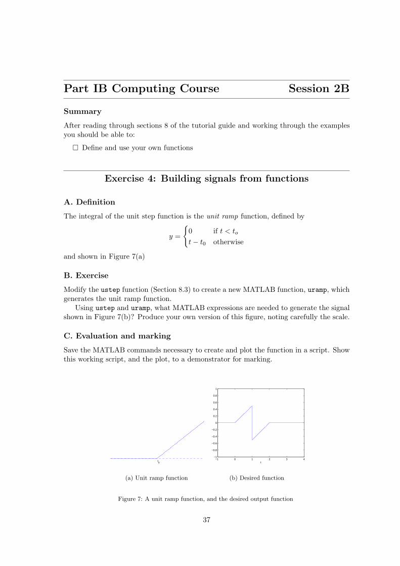
The integral of the unit step function is the unit ramp function, defined by

y =

{0 if t < to

t− t0 otherwise

and shown in Figure 7(a)

B. Exercise

Modify the ustep function (Section 8.3) to create a new MATLAB function, uramp, whichgenerates the unit ramp function.

Using ustep and uramp, what MATLAB expressions are needed to generate the signalshown in Figure 7(b)? Produce your own version of this figure, noting carefully the scale.

C. Evaluation and marking

Save the MATLAB commands necessary to create and plot the function in a script. Showthis working script, and the plot, to a demonstrator for marking.

t0

(a) Unit ramp function

−1 0 1 2 3 4−1

−0.8

−0.6

−0.4

−0.2

0

0.2

0.4

0.6

0.8

1

t

(b) Desired function

Figure 7: A unit ramp function, and the desired output function

37

9 Matrices and vectors

Vectors are special cases of matrices. A matrix is a rectangular array of numbers, the sizeof which is usually described as m × n, meaning that it has m rows and n columns. Forexample, here is a 2× 3 matrix:

A =[

5 7 9−1 3 −2

]

To enter this matrix into MATLAB you use the same syntax as for vectors, typing it inrow by row:

>> A=[5 7 9-1 3 -2]

A =5 7 9

-1 3 -2>>

alternatively, you can use semicolons to mark the end of rows, as in this example:

>> B=[2 0; 0 -1; 1 0]B =

2 00 -11 0

You can also use the colon notation, as before:

>> C = [1:3; 8:-2:4]C =

1 2 38 6 4

A final alternative is to build up the matrix row-by-row (this is particularly good forbuilding up tables of results in a for loop):

>> D=[1 2 3];>> D=[D; 4 5 6];>> D=[D; 7 8 9]D =

1 2 34 5 67 8 9

9.1 Matrix multiplication

With vectors and matrices, the * symbol represents matrix multiplication, as in theseexamples (using the matrices defined above)

38

>> A*Bans =

19 -7-4 -3

>> B*Cans =

2 4 6-8 -6 -41 2 3

>> A*C??? Error using ==> *Inner matrix dimensions must agree.

You might like to work out these examples by hand to remind yourself what is going on.Note that you cannot do A*C, because the two matrices are incompatible shapes.11

When just dealing with vectors, there is little need to distinguish between row andcolumn vectors. When multiplying vectors, however, it will only work one way round. Arow vector is a 1× n matrix, but this can’t post-multiply a m× n matrix:

>> x=[1 0 3]x =

1 0 3>> A*x??? Error using ==> *Inner matrix dimensions must agree.

9.2 The transpose operator

Transposing a vector changes it from a row to a column vector and vice versa. The trans-pose of a matrix interchanges the rows with the columns. Mathematically, the transposeof A is represented as AT . In MATLAB an apostrophe performs this operation:

>> AA =

5 7 9-1 3 -2

>> A’ans =

5 -17 39 -2

11In general, in matrix multiplication, the matrix sizes are

(l ×m)*(m× n) → (l × n)

When we try to do A*C, we are attempting to do (2× 3)*(2× 3), which does not agree with the definitionabove. The middle pair of numbers are not the same, which explains the wording of the error message.

39

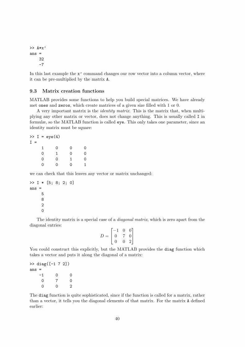
>> A*x’ans =

32-7

In this last example the x’ command changes our row vector into a column vector, whereit can be pre-multiplied by the matrix A.

9.3 Matrix creation functions

MATLAB provides some functions to help you build special matrices. We have alreadymet ones and zeros, which create matrices of a given size filled with 1 or 0.

A very important matrix is the identity matrix. This is the matrix that, when multi-plying any other matrix or vector, does not change anything. This is usually called I informulæ, so the MATLAB function is called eye. This only takes one parameter, since anidentity matrix must be square:

>> I = eye(4)I =

1 0 0 00 1 0 00 0 1 00 0 0 1

we can check that this leaves any vector or matrix unchanged:

>> I * [5; 8; 2; 0]ans =

5820

The identity matrix is a special case of a diagonal matrix, which is zero apart from thediagonal entries:

D =

−1 0 00 7 00 0 2

You could construct this explicitly, but the MATLAB provides the diag function whichtakes a vector and puts it along the diagonal of a matrix:

>> diag([-1 7 2])ans =

-1 0 00 7 00 0 2

The diag function is quite sophisticated, since if the function is called for a matrix, ratherthan a vector, it tells you the diagonal elements of that matrix. For the matrix A definedearlier:

40

>> diag(A)ans =

53

Notice that the matrix does not have to be square for the diagonal elements to be defined,and for non-square matrices it still begins at the top left corner, stopping when it runsout of rows or columns.

9.4 Building composite matrices

It is often useful to be able to build matrices from smaller components, and this can easilybe done using the basic matrix creation syntax:

>> comp = [eye(3) B;A zeros(2,2)]

comp =1 0 0 2 00 1 0 0 -10 0 1 1 05 7 9 0 0

-1 3 -2 0 0

You just have to be careful that each sub-matrix is the right size and shape, so that thefinal composite matrix is rectangular. Of course, MATLAB will tell you if any of themhave the wrong number of row or columns.

9.5 Matrices as tables

Matrices can also be used to simply tabulate data, and can provide a more natural wayof storing data:

>> t=0:0.2:1;>> freq=[sin(t)’ sin(2*t)’, sin(3*t)’]freq =

0 0 00.1987 0.3894 0.56460.3894 0.7174 0.93200.5646 0.9320 0.97380.7174 0.9996 0.67550.8415 0.9093 0.1411

Here the nth column of the matrix contains the (sampled) data for sin(nt). The alternativewould be to store each series in its own vector, each with a different name. You wouldthen need to know what the name of each vector was if you wanted to go on and use thedata. Storing it in a matrix makes the data easier to access.

41

9.6 Extracting bits of matrices

Numbers may be extracted from a matrix using the same syntax as for vectors, usingthe () brackets. For a matrix, you specify the row co-ordinate and then the columnco-ordinate (note that, in Cartesian terms, this is y and then x). Here are some examples:

>> J = [1 2 3 45 6 7 8

11 13 18 10];>> J(1,1)ans =

1>> J(2,3)ans =

7>> J(1:2, 4) %Rows 1-2, column 4ans =

48

>> J(3,:) %Row 3, all columnsans =

11 13 18 10

The : operator can be used to specify a range of elements, or if used just by itself then itrefers to the entire row or column.

These forms of expressions can also be used on the left-hand side of an expression towrite elements into a matrix:

>> J(3, 2:3) = [-1 0]J =

1 2 3 45 6 7 8

11 -1 0 10

10 Basic matrix functions

MATLAB allows all of the usual arithmetic to be performed on matrices. Matrix multipli-cation has already been discussed, and the other common operation is to add or subtracttwo matrices of the same size and shape. This can easily be performed using the + and -operators. As with vectors, MATLAB also defines the .* and ./ operators, which allowthe corresponding elements of two matching matrices to be multiplied or divided. All theelements of a matrix may be raised to the same power using the .^ operator.

Unsurprisingly, MATLAB also provides a large number of functions for dealing withmatrices, and some of these will be covered later in this tutorial. Try typing

help matfun

42

for a taster. For the moment we’ll consider some of the fundamental matrix functions.The size function will tell you the dimensions of a matrix. This is a function which

returns a vector, specifying the number of rows, and then columns:

>> size(J)ans =

3 4

The inverse of a matrix is the matrix which, when multiplied by the original matrix,gives the identity (AA−1 = A−1A = I). It ‘undoes’ the effect of the original matrix. It isonly defined for square matrices, and in MATLAB can be found using the inv function:

>> A = [3 0 40 1 -12 1 -3];

>> inv(A)ans =

0.1429 -0.2857 0.28570.1429 1.2143 -0.21430.1429 0.2143 -0.2143

>> A*inv(A) %Check the answerans =

1.0000 0.0000 -0.00000 1.0000 00 0.0000 1.0000

Again, note the few numerical errors which have crept in, which stops MATLAB fromrecognising some of the elements as exactly one or zero.

The determinant of a matrix is a very useful quantity to calculate. In particular, a zerodeterminant implies that a matrix does not have an inverse. The det function calculatesthe determinant:

>> det(A)ans =

-14

43

Part IB Computing Course Session 3A

Summary

After reading through sections 9 and 10 of the tutorial guide and working through theexamples you should be able to:

¤ Define matrices in MATLAB

¤ Use matrices and vectors in simple calculations

¤ Perform standard operations on matrices

Exercise 5: Euler angles

A. Theory

A rotation matrix in two dimensions is easy to define. There is only one axis of rotation,which is normal to the 2D plane, and a rotation of a positive angle θ (in a right-handedco-ordinate system) is given by the matrix

[cos θ − sin θsin θ cos θ

]

Defining rotations in three dimensions is more difficult. One method of defining rotationsis known as Euler angles, which are often used in mechanics.12

The method of Euler angles, specifies three angles. These are commonly called azimuth,elevation and roll (or in aeronautical terms yaw, pitch and roll). We shall label these threeangles as ψ, θ and φ, and our object exists in a normal right-handed co-ordinate set, x, yand z.

The rotations must be applied in a specific order. A point (x, y, z) is first rotated fromits original location by an angle ψ about the x axis (roll):

x′

y′

z′

=

1 0 00 cos ψ − sinψ0 sinψ cosψ

xyz

Then it is rotated by an angle θ about the original y axis (elevation):

x′′

y′′

z′′

=

cos θ 0 − sin θ0 1 0

sin θ 0 cos θ

x′

y′

z′

The final rotation, φ is then about the original z axis (azimuth), defining the new locationx′′′, y′′′ and z′′′ as

x′′′

y′′′

z′′′

=

cosφ − sinφ 0sinφ cosφ 0

0 0 1

x′′

y′′

z′′

12Named after the same Leonhard Euler (1707–1783) responsible for the method of finding π that wasconsidered in the IA C++ computing course.

44

B. Computing exercise

Write a MATLAB that function which takes three Euler angles and produces a single 3Drotation matrix, transforming points (x, y, z) to (x′′′, y′′′, z′′′), as defined above.

Use this function to find the rotation matrix R which rotates a co-ordinate system bythe Euler angles (90◦, 20◦, 15◦). Verify that this is a valid rotation matrix i.e. that it isorthogonal, and has a determinant of +1.

The point p is to be mapped to a new location p0 using your matrix R. If p = (2, 3, 0)T ,what is p0? What matrix reverses this transformation?

Find the matrix S which represents the rotation given by (−90◦,−20◦,−15◦). To wheredoes your transformed point p0 map under this new rotation? Why is S is not the reverseof R?

C. Implementation notes

1. Degrees and radiansRemember that MATLAB works in radians, not degrees. You might like to makeuse of the sind function you defined earlier, and also to define a cosd function.

D. Evaluation and marking

Write a MATLAB script which uses your Euler angle function to perform all the calcula-tions necessary for the exercise. Show this working script, and your Euler angle functionto a demonstrator for marking.

45

11 Solving Ax = b

One of the most important use of matrices is for representing and solving simultaneousequations. A system of linear equations is

a11x1 + a12x2 + · · ·+ a1nxn = b1

a21x1 + a22x2 + · · ·+ a2nxn = b2

... =...

am1x1 + am2x2 + · · ·+ amnxn = bm

where the aij and bi are known, and we are looking for a set of values xi that simultaneouslysatisfy all the equations. This can be written in matrix-vector form as

a11 a12 · · · a1n

a21 a22 · · · a2n...

.... . .

...am1 am2 · · · amn

x1

x2...

xn

=

b1

b2...

bm

or

Ax = b

In this representation, A is the matrix of coefficients, b are the constants, and x is thevector of parameters that we want to find.

Since MATLAB is designed to process matrices and vectors, it is particularly appro-priate to use it to solve these forms of problems.

11.1 Solution when A is invertible

The simplest set of linear equations to solve occur when you have both n equations and nunknowns. In this case the matrix A will be square and can often be inverted. Considerthis simple example:

x + y = 32x− 3y = 5

Solving this in MATLAB is a case of turning the equations into matrix-vector form andthen using the inverse of A to find the solution:

>> A=[1 12 -3];

>> b=[3 5]’;>> inv(A)*bans =

2.80000.2000

>> A*ans %Just to checkans =

3.00005.0000

So the solution is x = 2.8, y = 0.2.

46

11.2 Gaussian elimination and LU factorisation

Calculating the inverse of a matrix is an inefficient method of solving these problems, evenif MATLAB can still invert large matrices a lot more quickly than you could do by hand.From the IB Linear Algebra course, you should be familiar with Gaussian elimination, andLU factorisation (which is just Gaussian elimination in matrix form).13 These provide amore efficient way of solving Ax = b, and MATLAB makes it very easy to use Gaussianelimination by defining this as the meaning of matrix division for invertible matrices.

11.3 Matrix division and the slash operator

In a normal algebraic equation, ax = b, if you want to find the value of x you would justcalculate x = b/a. In a matrix-vector equation Ax = b, however, division is not definedand the solution is given by x = A−1b. As a shortcut for this, MATLAB defines a specialoperator \ (note that this is a backslash, not the divide symbol), and can be thought ofas ‘matrix division’. Using this, the solution to our earlier equation may be calculated as:

>> A\bans =

2.80000.2000

Note that this is not a standard notation and in written mathematical expressions youshould still always write A−1b.

You should recall that matrix multiplication is not commutative i.e. AB 6= BA. Thismeans that, while the solution to AX = B is given by X = A−1B, the solution to XA = Bis X = BA−1, and these two expressions are different. As a result, MATLAB also definesthe / (forward slash) operator which performs this other variety of matrix division. Theformer case, however, is more likely, and it is usually the backslash that you will need touse. The two slash operators are summarised in Table 5.

operator to solve MATLAB mathematical namecommand equivalent

\ AX = B A\B A−1B left division (backslash)/ XA = B B/A BA−1 right division (forward slash)

Table 5: Summary of MATLAB’s slash operators. These use Gaussian elimination if the matrix is invert-ible, and finds the least squares solution otherwise.

11.4 Singular matrices and rank

The slash operator tries to do its best whatever matrix and vector it is given, even if asolution is not possible, or is undetermined. Consider this example:

u + v + w = 22u + 3w = 5

3u + v + 4w = 6

13The lu function in MATLAB will perform the LU factorisation of a matrix for you (see the helpmessage for that function).

47

This is again an equation of the form Ax = b. If you try to solve this in MATLAB usingthe slash operator, you get

>> A=[1 1 12 0 33 1 4];

>> b=[2 5 6]’;>> x=A\bx =1.0e+015 *-5.40431.80143.6029

>> A*x %Should be the same as bans =

266

So the solution given is not a solution to the equation! You should perhaps have beensuspicious, anyway, from the size of the numbers in x. What has gone wrong?

In this case the matrix A is singular. This means that it has a zero determinant, andso is non-invertible. We can check this by typing

>> det(A)ans =

0

When the matrix is singular it means that there is not a unique solution to the equations.But we have three equations and three unknowns, so why is there not a unique solution?The problem is that there are not three unique equations. The rank function in MATLABestimates the rank of a matrix—the number linearly of independent rows or columns inthe matrix:

>> rank(A)ans =

2

So there are only two independent equations in this case. Looking at the original equationsmore carefully, we can see that the first two add to give 3u + v + 4w = 7, which isclearly inconsistent with the third equation. In other words, there is no solution to thisequation. What has happened in this case is that, thanks to rounding errors in theGaussian elimination, MATLAB has found an incorrect solution.

The moral of this section is that the slash operator in MATLAB is very powerful anduseful, but you should not use it indiscriminately. You should check your matrices toensure that they are not singular, or near-singular.14

14Some singular matrices can have an infinity of solutions, rather than no solution. In this case, theslash operator gives just one of the possible values. This again is something that you need to be aware of,and watch out for.

48

11.5 Ill-conditioning

Matrices which are near-singular are an example of ill-conditioned matrices. A problem isill-conditioned if small changes in the data produce large changes in the results. Considerthis system: [

1 11 1.01

] (11

)=

(2

2.01

)

for which MATLAB displays the correct answer:

>> M=[1 1; 1 1.01]; b=[2; 2.01];>> x=M\bx =

1.00001.0000

Let us now change one of the elements of M by a small amount, and see what happens:

>> M(1,2) = 1.005;>> M\bans =

-0.01002.0000

Changing this one element by 0.5% has decreased X(1) by approximately 101%, andincreased X(2) by 100%!

The sensitivity of a matrix is estimated using the condition number, the precise def-inition of which is beyond the scope of this tutorial. However, the larger the conditionnumber, the more sensitive the solution is. In MATLAB, the condition number can befound by the cond function:

>> cond(M)ans =402.0075

A rule of thumb is that if you write the condition number in exponential notation a×10k,then you last k significant figures of the result should be ignored. MATLAB works to aboutfifteen significant figures, so the number of significant figures that you should believe is(15− k). In this example, the condition number is 4× 102, so all of the the last 2 decimalplaces of the solution should be dropped i.e. the result is perfectly valid.15 For the singularmatrix A from earlier, which gave the spurious result, cond gives a condition number of2.176× 1016. In other words, all of the result should be ignored!16

15This assumes that the values entered into the original matrix M and vector b were accurate to fifteensignificant figures. If those values were known to a lesser accuracy, then you lose k significant figures fromthat accuracy.

16The condition number for this singular matrix again shows one of the problems of numerical compu-tations. All singular matrices should have a condition number of infinity.

49

−4 −3 −2 −1 0 1 2 3 4−10

−5

0

5

10

15

20

x

y

2x − y = 2

x + y = 5

6x − y = −5

Figure 8: Three lines and the least squares estimate of the common intersection point

11.6 Over-determined systems: Least squares

A common experimental scenario is when you wish to fit a model to a large number ofdata points. Each data point can be expressed in terms of the model’s equation, giving aset of simultaneous equations which are over-determined i.e. the number of independentequations, m, is larger than the number of variables, n. In these cases it is not possibleto find an exact solution, but the desired solution is the ‘best fit’. This is usually definedas the model parameters which minimise the squared error to each data point.

For a set of equations which can be written as Ax = b, the least-squares solution isgiven by the pseudoinverse (see your IB Linear Algebra notes):

x =(ATA

)−1ATb

In MATLAB you can again use the \ operator. For invertible matrices it is defined tosolve the equation using Gaussian elimination, but for over-determined systems it findsthe least squares solution. The pseudoinverse can also be calculated in MATLAB usingthe pinv function, as demonstrated in the following example.

11.7 Example: Triangulation

A hand-held radio transmitter is detected from three different base stations, each of whichprovide a reading of the direction to the transmitter. The vector from each base station isplotted on a map, and they should all meet at the location of the transmitter. The threelines on the map can be described by the equations

2x− y = 2x + y = 5

6x− y = −5

and these are plotted in Figure 8. However, because of various errors, there is not onecommon point at which they meet.

The least squares solution to the intersection point can be calculated in MATLAB ina number of different ways once we have defined our matrix equation:

50

>> A=[2 -1; 1 1; 6 -1];>> b = [2 5 -5]’;>> x = inv(A’*A)*A’*bx =

-0.09462.4459

>> x=pinv(A)*bx =

-0.09462.4459

>> x = A\bx =

-0.09462.4459

All of these, of course, give the same solution. This least squares solution is marked onFigure 8 with a ‘*’.

12 More graphs

MATLAB provides more sophisticated graphing capabilities than simply plotting 2DCartesian graphs. It can also produce histograms, 3D surfaces, contour plots and po-lar plots, to name a few. Details of all of these can be found in the help system (underthe subjects graph2d and graph3d), and only a few examples will be considered here.

12.1 Putting several graphs in one window

If you have several graphs sharing a similar theme, you can plot them on separate graphswithin the same graphics window. The subplot command splits the graphics window intoan array of smaller windows. The general format is

subplot(rows ,columns ,select )

The select argument specifies the current graph in the array. These are numbered fromthe top left, working along the rows first. The example below creates two graphs, one ontop of the other, as shown in Figure 9.

>> x = linspace(-10, 10);>> subplot(2,1,1) % Specify two rows, one column, and select>> % the top one as the current graph>> plot(x, sin(x));>> subplot(2,1,2);>> plot(x, sin(x)./x));

The standard axes labelling and title commands can also be used in each subplot.

51

−10 −8 −6 −4 −2 0 2 4 6 8 10−1

−0.5

0

0.5

1

−10 −8 −6 −4 −2 0 2 4 6 8 10−0.4

−0.2

0

0.2

0.4

0.6

0.8

1

Figure 9: Example of the subplot command, showing a sine and sinc curve one above the other.

−1

−0.5

0

0.5

1

−1

−0.5

0

0.5

10

5

10

15

20

25

30

35

xy

z

Figure 10: Example of the plot3 command, showing a helix.

12.2 3D plots

MATLAB provides a wide range of methods for visualising 3D data. The simplest formof 3D graph is plot3, which is the 3D equivalent of the plot command. Used for plottingpoints or drawing lines, this simply takes a list of x, y and z values. The following exampleplots a helix, using a parametric representation.17

>> t = 0:pi/50:10*pi;>> x = sin(t); y = cos(t); z = t;>> plot3(x, y, z);

The graph is shown in Figure 10. The xlabel and ylabel commands work as before, andnow the zlabel command can also be used. When plotting lines or points in 3D you canuse all of the styles listed in Table 3.

17A line is only a one dimensional shape—you can define a point along its length, but it has no width orheight. Lines can therefore be described in terms of only one parameter: the distance along the line. Thex, y (and in 3D z) co-ordinates of points on the line can all be written as functions of this distance alongthe line: ‘if I am this far along the line, I must be at this point.’

52

12.3 Changing the viewpoint

If you want to rotate the 3D plot to view it from another angle, the easiest method is topress the ª button on the figure’s toolbar. Clicking and dragging with the mouse on theplot will now rotate it. It helps if you have labelled the axes before you do this, in caseyou lose track of where you are!

The MATLAB command view can be used to select a particular viewpoint. Look itup on the help system for more information.

12.4 Plotting surfaces

Another common 3D graphing requirement is to plot a surface, defined as a function oftwo variables f(x, y), and these can be plotted in a number of different ways in MATLAB.First, though, in order to plot these functions we need a grid of points at which the functionis to be evaluated. Such a grid can be created using the meshgrid function:

>> x = 2:0.2:4; % Define the x- and y- coordinates>> y = 1:0.2:3; % of the grid lines>> [X,Y] = meshgrid(x, y); %Make the grid

The matrices X and Y then contain the x and y coordinates of the sample points. Thefunction can then be evaluated at each of these points. For example, to plot

f(x, y) = (x− 3)2 − (y − 2)2

over the grid calculated earlier, you would type

>> Z=(X-3).^2 - (Y-2).^2;>> surf(X,Y,Z)

surf is only one of the possible ways of visualising a surface. Figure 11 shows, in thetop left, this surface plotted using the surf command, and also the results of some of theother possible 3D plotting commands.

12.5 Images and Movies

An image is simply a matrix of numbers, where each number represents the colour orintensity of that pixel in the image. It should be no surprise, therefore, that MATLAB canalso perform image processing. There are several example images supplied with MATLAB,and the following commands load and display one of them:

>> load gatlin>> colormap(gray(64)) % Tell MATLAB to expect a greyscale image>> image(X)

The file gatlin.mat contains the matrix X. If you look at the elements of this matrix, youwill see that it simply contains numbers between 0 and 63, which represent the brightnessof each pixel (0 is black and 63 is white). The image command displays this matrix asan image; the colormap command tells MATLAB to interpret each number as a shade ofgrey, and what the range of the numbers is.18

18Try colormap(jet) for an example of an alternative interpretation of the numbers (this is the defaultcolormap). The colormap is also used to determine the colours for the height in the 3D plotting commands.

53

23

4

1

2

3−1

0

1

surf

23

4

1

2

3−1

0

1

mesh

23

4

1

2

3−1

0

1

meshz

2 2.5 3 3.5 41

1.5

2

2.5

3contour

Figure 11: Examples of the same saddle-shaped surface visualised using different MATLAB commands.(The 4 graphs are plotted in the same figure using the command subplot(2,2,i ).)

MATLAB can also create and display movies. These are stored in a special format,but you can turn the current figure into a movie frame by using

M(frame_no ) = getframe;

or movie frames can also be created directly from an image matrix:

M(frame_no ) = im2frame(im , colormap_name );

Once you have built up a movie, it can be played using the movie command:

movie(M)

The optional Exercise 7 in this tutorial will consider images and movies.

54

Part IB Computing Course Session 3B

Summary

After reading through Sections 11 and 12 of the tutorial guide and working through theexamples you should be able to:

¤ Write linear simultaneous equations in matrix-vector form

¤ Use the slash operator in MATLAB to solve Ax = b

¤ Understand what the slash operator does in different scenarios

¤ Appreciate the problems of ill-conditioned matrices

¤ Produce more advanced figures, including displaying three-dimensional data

Exercise 6: Leg Before Wicket?

A. Description

The Leg Before Wicket (LBW) rule in the game of cricket is the cause of many contentiousdecisions, but the problem is a very simple one: if the batsman had not got in the way,would the ball have hit the stumps? This is an extrapolation problem. We can track theball’s position from the point it bounces, until it hits the batsman, and the problem isthen just one of fitting a curve to the observed trajectory and extrapolating this to see ifit hits the stumps.

A tracking system measures the ball’s position at a rate of 150Hz, and for each samplestores the x, y and z co-ordinate of the ball. Measurements are in metres, according to theaxes defined in Figure 12, centred on the bottom of the middle stump. The ball’s positionis accurate to about 2cm.

Figure 12: Definition of axes, and dimensions of the stumps

55

B. Exercise

The file cricket.txt contains data from a disputed decision, to be analysed by thissystem. The file contains 4 columns of data, in the format (time x y z ). Load this fileinto MATLAB and produce a three dimensional plot of the position data, marking eachsample with a blob.

Assuming a linear horizontal trajectory (i.e. that the ball’s velocity is constant in xand y), and that its height describes a parabola, express each of the three co-ordinates asa function of time. Use least squares to estimate the motion parameters and so fit a curveto the sample points. You should not assume you know the value of the acceleration due togravity, g, and you should instead include this as one of your unknown parameters. Whatvalue for g is given by this model? Add your estimated curve to the 3D plot, extrapolatingit past the stumps.

Fit another curve by least squares, this time assuming that g = 9.81, and add this toyour plot in a different colour. Do you notice a significant difference? Using this model ofthe ball’s trajectory, what was the velocity of the ball when t = 0? Finally, calculate theball’s position as it passes the stumps. Would the ball have hit the stumps?

C. Implementation notes

1. Solving equations of motion by least squaresFor each sample point you can write three equations in terms of time: one for x, onefor y, and one for z. The first two are linear, in the form

x = x0 + uxt

And similarly for y. Each of these equations has two parameters, the speeds ux

and uy, and the initial positions x0 and y0. The z motion will have an additionalquadratic term involving g:

z = z0 + uzt + 12gt2

If g is unknown (as in the first part of this exercise), then this has three unknownparameters, giving seven parameters in total. The three equations may be writtenin matrix-vector form as

xyz

=

A

ux

uy

uz

x0

y0

z0

g

where the elements in A are given by a straightforward comparison of coefficientswith the three motion equations.

Each sample point gives different values of x, y and z, and so three different equa-tions. Each of these equations gives different values for the matrix A, but the param-eters ux etc. stay exactly the same (these are our initial conditions, and define the

56

fitted trajectory). We can therefore stack all of our equations on top of each otherto create some huge matrices and vectors:

x1

y1

z1

x2

y2

z2...

xn

yn

zn

=

A1

A2

...

An

ux

uy

uz

x0

y0

z0

g

This then an over-determined equation of the form Ax = b, and can be solved inMATLAB with the slash operator or the pseudoinverse.

In the second part, when g is known, there are only six unknown parameters, andso your parameter vector will be

(ux uy uz x0 y0 z0)T

You will therefore need a different matrix A and vector b.

2. Building the matrix AEach data point from the text file contributes three equations, and so three lines toboth A and b. The best way to build this matrix and vector is with a for loop whichsteps through the rows of the raw data and, for each row, fills in three rows of A andb. A row i from the text file (i = 1 . . . n) provides information for rows 3(i− 1) + 1,3(i− 1) + 2 and 3(i− 1) + 3 of this matrix and vector.

3. The position of the stumpsThe dimensions of the stumps are given in Figure 12. In addition, the scriptstumps.m will draw a representation of the stumps in a 3D figure window.

D. Evaluation and marking

Write a MATLAB script that contains all the commands necessary for this exercise, sothat it displays the required numbers and plots the graphs. Use an if statement to printout a message saying whether the ball would have hit the stumps. Show this workingscript to a demonstrator for marking.

Once you have finished this exercise and had it marked, you have qualified for your fulltwelve marks. This exercise must be marked by the end of your fourth session.

You should now read through the rest of this tutorial and, if you have time left, shouldattempt Exercise 7.

57

13 Eigenvectors and the Singular Value Decomposition

After the solution of Ax = b, the other important matrix equation is Ax = λx, the solutionsto which are the eigenvectors and eigenvalues of the matrix A. Equations of this form cropup often in engineering applications, and MATLAB again provides the tools to solve them.

13.1 The eig function

The eig function in MATLAB calculates eigenvectors and eigenvalues. If used by itself,it just provides a vector containing the eigenvalues, as in this example:

>> A=[1 3 -23 5 1-2 1 4];

>> eig(A)ans =

6.60764.9045-1.5120

In order to obtain the eigenvectors, you need to provide two variables for the answer:

>> [V,D]=eig(A)V =

0.4804 0.3153 0.81840.8764 -0.2071 -0.4347-0.0324 -0.9261 0.3758

D =6.6076 0 0

0 4.9045 00 0 -1.5120

The columns of the matrix V are the eigenvectors, and the eigenvalues are this time re-turned in a diagonal matrix. The eigenvectors and eigenvalues are returned in this formatbecause this is then consistent with the diagonal form of the matrix. You should recallthat, if U is the matrix of eigenvectors and Λ the diagonal matrix of eigenvalues, thenA = UΛU−1. We can easily check this using the matrices returned by eig:

>> V*D*inv(V)ans =

1.0000 3.0000 -2.00003.0000 5.0000 1.0000-2.0000 1.0000 4.0000

which is the original matrix A.

13.2 The Singular Value Decomposition

Eigenvectors and eigenvalues can only be found for a square matrix, and thus the decom-position into UΛU−1 is only possible for these matrices. The Singular Value Decomposition

58

(SVD) is a very useful technique, which provides a similar decomposition for any matrix.The specifics are covered in the IB Linear Algebra course, but an outline of the outcomeof the decomposition is given here.

The SVD takes an m× n matrix A and factors it into A = Q1ΣQT2 , where

• Q1 is an m×m orthogonal matrix whose columns are the eigenvectors of AAT

• Q2 is an n× n orthogonal matrix whose columns are the eigenvectors of ATA

• Σ is an m×n diagonal matrix whose elements are the square roots of the eigenvaluesof AAT and ATA (both have the same eigenvalues, but different eigenvectors)

This is better shown graphically:

A

·m

· · n · ·

=

Q1

·m

· m ·

Σ

·m

· · n · ·

QT2

··n·

· · n · ·

The most important part of this decomposition to consider is the matrix Σ, the diagonalmatrix, whose elements are called the singular values, σi:

Σ =

σ1

σ2

. . . 0σr

0

0. . .

0

Being part of a diagonal matrix, these only multiply particular columns of Q1 or Q2.19 Thesize of the singular value tells you exactly how much influence the corresponding rows andcolumns of Q1 and QT

2 have over the original matrix. Clearly, if a singular value is tiny,very little of the corresponding rows and columns get added into the matrix A when it isreconstituted. It is quite common for a matrix to have some zero eigenvalues, as shownabove. These zero elements on the diagonal indicate correspond to rows or columns thatgive no extra information. This indicates, of course, that not all of the matrix is useful—that it is rank deficient. Or, in terms of simultaneous equations, that not all the equationsare independent.

The SVD is a very useful tool for analysing a matrix, and the solutions to manyproblems can simply be read off from the decomposed matrices. For example, the nullspaceof the matrix (the solution to Ax = 0) is simply the columns of Q2 which correspond tothe zero singular values. The SVD is also highly numerically stable—matrices which areslightly ill-conditioned stand more chance of working with SVD than with anything else.

19The singular values Σ of course multiply the rows of QT2 , and hence the columns of the un-transposed

version, Q2.

59

13.3 Approximating matrices: Changing rank

Another important use of the SVD is the insight it gives into how much of a matrix isimportant, and how to simplify a matrix with minimal disruption. The singular values areusually arranged in order of size, with the first, σ1, being the largest and most significant.The corresponding columns of Q1 and Q2 are therefore also arranged in importance. Whatthis means is that, while we can find the exact value of A by multiplying Q1ΣQ

T2 , if we

removed (for example) the last columns of Q1 and Q2, and the final singular value, wewould be removing the least important data. If we then multiplied these simpler matrices,we would only get an approximation to A, but one which still contained all but the mostinsignificant information. Exercise 7 will consider this in more detail.

13.4 The svd function

The SVD is performed in MATLAB using the svd function. As with the eig function, byitself it only returns the singular values, but if given three matrices for the answer then itwill fill them in with the full decomposition:

>> A =[ 1 3 -2 33 5 1 5-2 1 4 2];

>> svd(A)ans =

8.93105.04121.6801

>> [U,S,V] = svd(A,0)U =

0.4673 -0.3864 -0.79520.8621 -0.0003 0.50680.1961 0.9223 -0.3329

S =8.9310 0 0 0

0 5.0412 0 00 0 1.6801 0

V =0.2980 -0.4428 0.8280 -0.17190.6616 -0.0473 -0.1097 0.74030.0797 0.8851 0.4556 0.05290.6835 0.1356 -0.3079 -0.6478

>>>> U*S*V’ %Check the answerans =

1.0000 3.0000 -2.0000 3.00003.0000 5.0000 1.0000 5.0000-2.0000 1.0000 4.0000 2.0000

Note that MATLAB automatically orders the singular values in decreasing order.

60

13.5 Economy SVD

If a m× n matrix A is overdetermined (i.e. m > n), then the matrix of singular values, Σ,will have at least one row of zeros:

>> A=[1 23 45 6];

>> [U,S,V] = svd(A)U =

0.2298 0.8835 0.40820.5247 0.2408 -0.81650.8196 -0.4019 0.4082

S =9.5255 0

0 0.51430 0

V =0.6196 -0.78490.7849 0.6196

If we then consider the multiplication A = U*S*V’, we can see that the last column of Userves no useful purpose—it multiplies the zeros in S, and so might as well not be there.Therefore this last column may be safely ignored, and the same is true of the last row ofS. What we are then left with is matrices of the following form:

A

··m·

· n ·

=

Q1

··m·

· n ·

Σ

·n

· n ·

QT2

·n

· n ·

MATLAB can be asked to perform this ‘economy’ SVD by adding ‘,0’ to the functionargument (NB this is a zero, not the letter ‘O’):

>> [U,S,V] = svd(A,0)U =

0.2298 0.88350.5247 0.24080.8196 -0.4019

S =9.5255 0

0 0.5143V =

0.6196 -0.78490.7849 0.6196

This is highly recommended for matrices of this shape, since it takes far less memory andtime to process.

61

Part IB Computing Course Session 4

Summary

After reading through Sections 13 of the tutorial guide and working through the examplesyou should be able to:

¤ Calculate eigenvectors and eigenvalues using MATLAB

¤ Have an understanding of what the Singular Value Decomposition (SVD) tells youabout a matrix

¤ Be able to perform the SVD in MATLAB

Exercise 7: Video textures (optional)

A. Theory

A video frame contains an enormous amount of data—for example a small video frame of100× 100 pixels still contains 10,000 elements of information. However, in a typical videoof an object, one needs nowhere near this many pieces of information to talk about what’sgoing on. Figure 13 shows part of a video of a fountain. If we wanted to describe thisfountain to someone else, we wouldn’t describe every pixel. We would say ‘it’s a smallfountain’, and could perhaps describe each frame by saying how strong the fountain wasat that instant.

Figure 13: The first four frames of the ‘fountain’ video sequence

What has been described in vague terms is two different state vectors for this videosequence. The current state of the image can be described as a list of numbers, whichrepresent the pixel intensities. But the current state of the fountain could be describedin terms of how strong the flow is, and exactly which way the wind is blowing, and othersuch descriptions. Such a description, in terms of fountain characteristics, is a much morecompact representation. What is needed, however, is the ability to translate from onestate representation to the other, so that given a fountain state vector (i.e. a descriptionof what the fountain is doing), we can create an image state vector (i.e. what the fountainlooks like). This can easily be written in matrix-vector terms:

y(t) = Cx(t)

where y(t) is the vector describing the image pixels at time t, x(t) is the (much smaller)description of the current fountain state. The matrix C is the mapping which knows how

62

to convert the state (e.g. ‘a fountain that’s a bit stronger than usual at the moment’) intothe image vector.

What we want to find is a single matrix C that will do this job—a matrix whichknows everything about fountains that’s needed for the sequence. In this way, rather thanstoring every video frame, we can instead just store this matrix and then each frame canbe described by it’s short fountain state vectors.

So, how do we find C or, indeed, the best fountain state vector x(t)? The first thingto do is to to represent each image as vector. Rather than having a matrix of numbers,we just want to turn it into a long list, perhaps produced by scanning each row in turn.This can be done in MATLAB using the : operator, as explained in the implementationnotes. This turns each image into a vector y(t). Our fountain state vector is already avector, y(t).

We want to analyse all the frames together, so let’s start by stacking them column bycolumn to make a matrix:

Y =[y(1) y(2) · · · y(τ)

]

X =[x(1) x(2) · · · x(τ)

]

Because these are just all the state vectors stacked together, and the same translation Cworks for all of them, we can then write20

Y = CX

What is therefore needed is some sensible way of dividing our known image data matrix,Y, into two matrices: one common translation matrix C, and the matrix of fountain states.There are many possible ways, but it turns out that the optimum approach is to use theSVD.21

Performing SVD on Y gives:Y = USVT

and we will choose to simply assign C and X from this decomposition:

C = U

X = SVT

In graphical terms, this gives (using the economy SVD since the number of image pixels,N is greater than the number of frames, τ):

Y

···N··

· · τ · ·

=

U

···N··

· · τ · ·

S

··τ·

· · τ · ·

VT

··τ·

· · τ · ·

20This is a useful general trick if you want to perform the same operation on a number of vectors.21This should be an obvious choice in any case, since the SVD is the most numerically stable of the

common decompositions, and so is the answer in most problems.

63

Thus far this is not a great saving, but now we can use the approximating power of theSVD to remove some dimensions (see Section 13.3). We have τ singular values, but let uschoose to keep only the n best. This equates to deleting the last τ − n columns of U, thelast τ − n rows and columns of S, and the last τ − n columns of V (or rows of VT ). Thisleaves us with

Y

···N··

· · τ · ·

=

U

···N··

· n ·

S

·n

· n ·

VT

·n

· · τ · ·

and hence, writing C = U and X = SVT :

Y

···N··

· · τ · ·

=

C

···N··

· n ·

X

·n

· · τ · ·

Which is what we were after. There is a different column of X for each time instant, andeach of these vectors is short—only n elements long. Each of these is translated througha matrix C to give the final video sequence, where the image vectors are N numbers long.

B. Exercise

Load the MATLAB file fountain.mat. This contains the ‘fountain’ sequence as a threedimensional array (see the implementation notes). Use the size command to see thedimensions of the image, and the number of frames. Write a function, playmovie, whichturns this 3D array into a MATLAB movie and plays it. Use this to see what the originalvideo looks like.

Write three further MATLAB functions:

• encodevideo: Converts the frames of the video into column vectors, and forms thematrix Y. Perform SVD on this matrix to give U, S and V.

• quantisevideo: Takes the three matrices, and a specified number of dimensions n,and removes the necessary rows and columns, returning the three modified matricesU, S and V.

• rebuildvideo: Takes the three matrices, multiplies them back together to give thereconstructed matrix Y. Then turns each of the columns of Y back into a matrix andbuilds a three-dimensional array holding the sequence.

64

First use the encodevideo and rebuildvideo functions pull apart and remake the video.Use playmovie on this new array to check that the reconstructed movie plays the sameas the original. Now try using quantisevideo between these two calls, setting n = 1to see what the video looks like with the very barest description of the fountain’s state.Try some other values of n to find out what kinds of motions you can get with differentnumbers of significant values.

Use trial and error to find the smallest value of n which gives a RMS pixel error, overthe whole sequence, of less than 5. With this value of n, how many numbers are neededto describe the matrices C and X. How does this compare with the number of numbers inthe original sequence? What is the compression ratio?

C. Implementation notes

1. Three dimensional arraysThe video file you will use is stored in a three dimensional array, [x, y, time ].Three dimensional arrays can be accessed exactly analogously to normal 2D matrices:if the array is called T, the first image in the sequence is T(:,:,1) i.e. all rows andall columns of the data at the first time instant.

2. Making moviesTo make a MATLAB movie, you need to write a for loop which steps through eachtime t step in the sequence, extracts the image, and calls

M(t) = im2frame(image , gray(256))

for each. Here, M is the movie you are building up, and t specifies the frame number.image is matrix which holds the image you want to use as that movie frame. theThe call to gray(256) makes a colormap with values from 0–255, which is the rangeof the intensities in the video sequence.

3. Turning matrices into vectors, and vice-versaYou will need to be able to turn an image matrix into a vector of numbers to makethe matrix Y. You can do this by typing

t = A(:)

The (:) tells MATLAB to turn the matrix A into a vector called t. Numbers areread into the vector column-by-column.To turn a vector back into a matrix, you need to have a matrix of the right sizeand shape into which the numbers will go. Otherwise, with just a vector, MATLABdoesn’t know how many rows and columns you want. Assuming that the matrix Bis the right size and shape,

B(:) = t

will put the vector t into B. You will have to pass the size (number of rows andcolumns) to your rebuildvideo function to allow it to reshape the vectors into thecorrectly-sized images.

65

4. Computation time

Calculating the SVD of a matrix of this size, or performing other calculations, doestake a good few seconds, so do not be surprised when you have to wait a little while.Please ensure, however, that you use the ‘economy’ SVD as described in Section13.5, as the full version takes a lot longer and also has a habit of consuming morememory than is available on these machines!

5. Calculating RMS error

To calculate the RMS difference between two matrices, you can first subtract thetwo matrices and square all the values (using the .^ operator). You can calculatethe sum of all the elements in a matrix A by using sum(sum(A)). The first call tosum totals up each column to give a vector of partial sums. The next call then addsup all the elements in that vector. After this, you just need to divide by the numberof elements, and find the square root.

D. Evaluation

Demonstrate your final encoded sequence to a demonstrator.

Additional: More video textures

A. What is the point of video textures?

The compression ratios possible using video texture techniques are far from stunning. Incontrast, the MPEG-2 compression used in DVDs uses a block-based JPEG-style com-pression, with motion prediction, and can reach compression ratios of 40:1. However,compression is not the main advantage of video textures. What this approach enables usto do is to synthesise novel videos of the object.

At the moment in computer-generated videos, and computer games, moving scenery(such as waves, or the fountain considered earlier) are poorly generated. They are producedeither by playing a short recorded sequence again and again, or by using very simple (andartificial-looking) model, which is again repeated ad infinitum. The problem of generatingtextures randomly is twofold: creating an image of a fountain at random involves knowinga lot about ‘fountain-ness’, and also that it must also be consistent with what’s happenedbefore—the fountain can’t suddenly jump from being very small to being very large. Thevideo texture approach knows about ‘fountain-ness’ in the matrix C, and it is much easierto randomly generate the small x vectors than a whole image. In fact, it is easy and fastenough to do this in real time.

B. Synthesising video textures

Synthesising a new fountain video is fairly simple given the video texture decomposition—it is just a case of creating a plausible new sequence of x vectors. There is not time inthis course to also go over the theory to do this, but a function randommovie has been

66

written, which performs this synthesises. Type help randommovie for information, oryou can have a look at the function in the editor if you are really interested to see how itworks. Try generating a new movie for your sequence.

C. More sequences

Two more sequence are provided for on which you can test your video texture functions:toilet.mat and steam.mat. Try your functions on these ones as well.

67

14 Complex numbers

Apart from matrix and vector computations, MATLAB also supports many other math-ematical and engineering concepts, and among these are complex numbers. Complexnumbers can be typed into MATLAB exactly as written, for example

>> z1=4-3iz1 =

4.0000 - 3.0000i

Alternatively, both i and j are initialised by MATLAB to be√−1 and so (if you’ve not

redefined them) you can also type

>> z2 = 1 + 3*jz2 =

1.0000 + 3.0000i

You can perform all the usual arithmetic operations on the complex numbers, exactlyas for real numbers:

>> z2-z1ans =-3.0000 + 6.0000i

>> z1+z2ans =

5>> z2/z1ans =-0.2000 + 0.6000i

>> z1^2ans =

7.0000 -24.0000i

MATLAB also provides some functions to perform the other standard complex numberoperations, such as the complex conjugate, or the modulus and phase of the number,and these are shown in Table 6. Other functions which have mathematical definitions forcomplex numbers, such as sin(x) or ex, also work with complex numbers:

>> sin(z2)ans =

8.4716 + 5.4127i>> exp(j*pi) %Should be 1ans =-1.0000 + 0.0000i

>> exp(j*2)ans =-0.4161 + 0.9093i

>> cos(2) + j*sin(2) %Should be the same as e^2ians =-0.4161 + 0.9093i

Matrices and vectors can, of course, also contain complex numbers.

68

function meaning definition (z = a + bi)imag Imaginary part areal Real part babs Absolute value (modulus) r = |z|conj Complex conjugate z = a− bi

angle Phase angle (argument) θ = tan−1(

ba

)

Table 6: Complex number functions

−5 −4 −3 −2 −1 0 1 2 3 4 5−5

−4

−3

−2

−1

0

1

2

3

4

5

(a) plot

1

2

3

4

5

30

210

60

240

90

270

120

300

150

330

180 0

(b) compass

Figure 14: Graphical representations of the complex numbers z1 = 4− 3i and z2 = 1 + 3i using the plot

and compass commands.

14.1 Plotting complex numbers

The plot command in MATLAB also understands complex numbers, so you can use thisto produce an Argand diagram (where the x-axis represents the real component and they-axis the imaginary):

>> plot(z1,’*’, z2,’*’)>> axis([-5 5 -5 5])

These commands produce the plot shown in Figure 14(a). This is not immediately clearsince it is difficult to tell where the origin is. You could also mark the origin, or drawlines from the origin to the numbers, but an alternative is to plot them using the compassfunction, as shown in Figure 14(b):

>> compass(z1)>> hold on>> compass(z2)

(The compass function can also plot ordinary 2D vectors, by giving an x and y displace-ment.)

69

14.2 Finding roots of polynomials

MATLAB provides a function, roots, which can be used to find the roots of polynomialequations. The equation is entered into MATLAB, surprise, surprise, using a vector forthe array of coefficients. For example, the polynomial equation

x5 + 2x4 − 5x3 + x + 3 = 0

would be represented as

>> c = [1 2 -5 0 1 3];

The roots function is then called using this vector:

>> roots(c)ans =-3.44731.1730 + 0.3902i1.1730 - 0.3902i

-0.4494 + 0.6062i-0.4494 - 0.6062i

15 Further reading

This tutorial guide has introduced the basic elements of using MATLAB. There are furtherguides available from CUED, which are available in the racks at the west end of the DPO:

• MATLAB by Example, G. Chand, T. Love, 1998

• Using Matlab at CUED, T. Love, 2000

• Getting started with Matlab, J.M. Maciejowski and T. Love, 2000

There are also many textbooks about MATLAB, and the following book is particularlyrecommended:

• Matlab 5 for engineers, A. Biran and M. Breiner, Addison-Wesley, 2000

The video texture work used for Exercise 7 is described in more detail in

• Dynamic Textures, S. Soatto, G. Doretto and Y.N. Wu, In Proceedings 8th Interna-tional Conference on Computer Vision, pages 436–446, Vancouver, July 2001

• http://vision.ucla.edu/projects/dynamic-textures.html

16 Acknowledgements

A brand new course like this is always a step into the unknown, and I hope there aren’ttoo many teething problems. My thanks go to Roberto Cipolla and Richard Prager forsharing their advice and experience, and to Maurice Ringer for drawing the cricket stumps.And to all of those who tested early versions of this for me.

The cricket example is based on David Mansergh’s 2000–2001 4th year project. Thevideo texture sequences are borrowed from Martin Szummer at MIT’s AI lab. Inspirationwas also drawn from various other MATLAB tutorials and text books.

70