part ia - vector calculus -...
TRANSCRIPT

Part IA — Vector Calculus
Based on lectures by B. AllanachNotes taken by Dexter Chua
Lent 2015
These notes are not endorsed by the lecturers, and I have modified them (oftensignificantly) after lectures. They are nowhere near accurate representations of what
was actually lectured, and in particular, all errors are almost surely mine.
Curves in R3
Parameterised curves and arc length, tangents and normals to curves in R3, the radiusof curvature. [1]
Integration in R2 and R3
Line integrals. Surface and volume integrals: definitions, examples using Cartesian,cylindrical and spherical coordinates; change of variables. [4]
Vector operatorsDirectional derivatives. The gradient of a real-valued function: definition; interpretationas normal to level surfaces; examples including the use of cylindrical, spherical *andgeneral orthogonal curvilinear* coordinates.
Divergence, curl and ∇2 in Cartesian coordinates, examples; formulae for these oper-ators (statement only) in cylindrical, spherical *and general orthogonal curvilinear*coordinates. Solenoidal fields, irrotational fields and conservative fields; scalar potentials.Vector derivative identities. [5]
Integration theoremsDivergence theorem, Green’s theorem, Stokes’s theorem, Green’s second theorem:statements; informal proofs; examples; application to fluid dynamics, and to electro-magnetism including statement of Maxwell’s equations. [5]
Laplace’s equationLaplace’s equation in R2 and R3: uniqueness theorem and maximum principle. Solutionof Poisson’s equation by Gauss’s method (for spherical and cylindrical symmetry) andas an integral. [4]
Cartesian tensors in R3
Tensor transformation laws, addition, multiplication, contraction, with emphasis on
tensors of second rank. Isotropic second and third rank tensors. Symmetric and
antisymmetric tensors. Revision of principal axes and diagonalization. Quotient
theorem. Examples including inertia and conductivity. [5]
1

Contents IA Vector Calculus
Contents
0 Introduction 4
1 Derivatives and coordinates 51.1 Derivative of functions . . . . . . . . . . . . . . . . . . . . . . . . 51.2 Inverse functions . . . . . . . . . . . . . . . . . . . . . . . . . . . 91.3 Coordinate systems . . . . . . . . . . . . . . . . . . . . . . . . . . 10
2 Curves and Line 112.1 Parametrised curves, lengths and arc length . . . . . . . . . . . . 112.2 Line integrals of vector fields . . . . . . . . . . . . . . . . . . . . 122.3 Gradients and Differentials . . . . . . . . . . . . . . . . . . . . . 142.4 Work and potential energy . . . . . . . . . . . . . . . . . . . . . . 15
3 Integration in R2 and R3 173.1 Integrals over subsets of R2 . . . . . . . . . . . . . . . . . . . . . 173.2 Change of variables for an integral in R2 . . . . . . . . . . . . . . 193.3 Generalization to R3 . . . . . . . . . . . . . . . . . . . . . . . . . 213.4 Further generalizations . . . . . . . . . . . . . . . . . . . . . . . . 24
4 Surfaces and surface integrals 264.1 Surfaces and Normal . . . . . . . . . . . . . . . . . . . . . . . . . 264.2 Parametrized surfaces and area . . . . . . . . . . . . . . . . . . . 274.3 Surface integral of vector fields . . . . . . . . . . . . . . . . . . . 294.4 Change of variables in R2 and R3 revisited . . . . . . . . . . . . . 31
5 Geometry of curves and surfaces 32
6 Div, Grad, Curl and ∇ 356.1 Div, Grad, Curl and ∇ . . . . . . . . . . . . . . . . . . . . . . . . 356.2 Second-order derivatives . . . . . . . . . . . . . . . . . . . . . . . 37
7 Integral theorems 387.1 Statement and examples . . . . . . . . . . . . . . . . . . . . . . . 38
7.1.1 Green’s theorem (in the plane) . . . . . . . . . . . . . . . 387.1.2 Stokes’ theorem . . . . . . . . . . . . . . . . . . . . . . . . 397.1.3 Divergence/Gauss theorem . . . . . . . . . . . . . . . . . 40
7.2 Relating and proving integral theorems . . . . . . . . . . . . . . . 41
8 Some applications of integral theorems 468.1 Integral expressions for div and curl . . . . . . . . . . . . . . . . 468.2 Conservative fields and scalar products . . . . . . . . . . . . . . . 478.3 Conservation laws . . . . . . . . . . . . . . . . . . . . . . . . . . 49
9 Orthogonal curvilinear coordinates 519.1 Line, area and volume elements . . . . . . . . . . . . . . . . . . . 519.2 Grad, Div and Curl . . . . . . . . . . . . . . . . . . . . . . . . . . 52
2

Contents IA Vector Calculus
10 Gauss’ Law and Poisson’s equation 5410.1 Laws of gravitation . . . . . . . . . . . . . . . . . . . . . . . . . . 5410.2 Laws of electrostatics . . . . . . . . . . . . . . . . . . . . . . . . . 5510.3 Poisson’s Equation and Laplace’s equation . . . . . . . . . . . . . 57
11 Laplace’s and Poisson’s equations 6111.1 Uniqueness theorems . . . . . . . . . . . . . . . . . . . . . . . . . 6111.2 Laplace’s equation and harmonic functions . . . . . . . . . . . . . 62
11.2.1 The mean value property . . . . . . . . . . . . . . . . . . 6211.2.2 The maximum (or minimum) principle . . . . . . . . . . . 63
11.3 Integral solutions of Poisson’s equations . . . . . . . . . . . . . . 6411.3.1 Statement and informal derivation . . . . . . . . . . . . . 6411.3.2 Point sources and δ-functions* . . . . . . . . . . . . . . . 65
12 Maxwell’s equations 6712.1 Laws of electromagnetism . . . . . . . . . . . . . . . . . . . . . . 6712.2 Static charges and steady currents . . . . . . . . . . . . . . . . . 6812.3 Electromagnetic waves . . . . . . . . . . . . . . . . . . . . . . . . 69
13 Tensors and tensor fields 7013.1 Definition . . . . . . . . . . . . . . . . . . . . . . . . . . . . . . . 7013.2 Tensor algebra . . . . . . . . . . . . . . . . . . . . . . . . . . . . 7113.3 Symmetric and antisymmetric tensors . . . . . . . . . . . . . . . 7213.4 Tensors, multi-linear maps and the quotient rule . . . . . . . . . 7313.5 Tensor calculus . . . . . . . . . . . . . . . . . . . . . . . . . . . . 74
14 Tensors of rank 2 7714.1 Decomposition of a second-rank tensor . . . . . . . . . . . . . . . 7714.2 The inertia tensor . . . . . . . . . . . . . . . . . . . . . . . . . . 7814.3 Diagonalization of a symmetric second rank tensor . . . . . . . . 80
15 Invariant and isotropic tensors 8115.1 Definitions and classification results . . . . . . . . . . . . . . . . 8115.2 Application to invariant integrals . . . . . . . . . . . . . . . . . . 82
3
0 Introduction IA Vector Calculus
0 Introduction
In the differential equations class, we learnt how to do calculus in one dimension.However, (apparently) the world has more than one dimension. We live in a3 (or 4) dimensional world, and string theorists think that the world has morethan 10 dimensions. It is thus important to know how to do calculus in manydimensions.
For example, the position of a particle in a three dimensional world can begiven by a position vector x. Then by definition, the velocity is given by d
dtx = x.This would require us to take the derivative of a vector.
This is not too difficult. We can just differentiate the vector componentwise.However, we can reverse the problem and get a more complicated one. We canassign a number to each point in (3D) space, and ask how this number changesas we move in space. For example, the function might tell us the temperature ateach point in space, and we want to know how the temperature changes withposition.
In the most general case, we will assign a vector to each point in space. Forexample, the electric field vector E(x) tells us the direction of the electric fieldat each point in space.
On the other side of the story, we also want to do integration in multipledimensions. Apart from the obvious “integrating a vector”, we might want tointegrate over surfaces. For example, we can let v(x) be the velocity of somefluid at each point in space. Then to find the total fluid flow through a surface,we integrate v over the surface.
In this course, we are mostly going to learn about doing calculus in manydimensions. In the last few lectures, we are going to learn about Cartesiantensors, which is a generalization of vectors.
Note that throughout the course (and lecture notes), summation conventionis implied unless otherwise stated.
4

1 Derivatives and coordinates IA Vector Calculus
1 Derivatives and coordinates
1.1 Derivative of functions
We used to define a derivative as the limit of a quotient and a function is differ-entiable if the derivative exists. However, this obviously cannot be generalizedto vector-valued functions, since you cannot divide by vectors. So we wantan alternative definition of differentiation, which can be easily generalized tovectors.
Recall, that if a function f is differentiable at x, then for a small perturbationδx, we have
δfdef= f(x+ δx)− f(x) = f ′(x)δx+ o(δx),
which says that the resulting change in f is approximately proportional to δx(as opposed to 1/δx or something else). It can be easily shown that the converseis true — if f satisfies this relation, then f is differentiable.
This definition is more easily extended to vector functions. We say a functionF is differentiable if, when x is perturbed by δx, then the resulting change is“something” times δx plus an o(δx) error term. In the most general case, δx willbe a vector and that “something” will be a matrix. Then that “something” willbe what we call the derivative.
Vector functions R→ Rn
We start with the simple case of vector functions.
Definition (Vector function). A vector function is a function F : R→ Rn.
This takes in a number and returns a vector. For example, it can map a timeto the velocity of a particle at that time.
Definition (Derivative of vector function). A vector function F(x) is differen-tiable if
δFdef= F(x+ δx)− F(x) = F′(x)δx+ o(δx)
for some F′(x). F′(x) is called the derivative of F(x).
We don’t have anything new and special here, since we might as well havedefined F′(x) as
F′ =dF
dx= limδx→0
1
δx[F(x+ δx)− F(x)],
which is easily shown to be equivalent to the above definition.Using differential notation, the differentiability condition can be written as
dF = F′(x) dx.
Given a basis ei that is independent of x, vector differentiation is performedcomponentwise, i.e.
Proposition.F′(x) = F ′i (x)ei.
Leibnitz identities hold for the products of scalar and vector functions.
5

1 Derivatives and coordinates IA Vector Calculus
Proposition.
d
dt(fg) =
df
dtg + f
dg
dtd
dt(g · h) =
dg
dt· h + g · dh
dtd
dt(g × h) =
dg
dt× h + g × dh
dt
Note that the order of multiplication must be retained in the case of the crossproduct.
Example. Consider a particle with mass m. It has position r(t), velocity r(t)and acceleration r. Its momentum is p = mr(t).
Note that derivatives with respect to t are usually denoted by dots insteadof dashes.
If F(r) is the force on a particle, then Newton’s second law states that
p = mr = F.
We can define the angular momentum about the origin to be
L = r× p = mr× r.
If we want to know how the angular momentum changes over time, then
L = mr× r +mr× r = mr× r = r× F.
which is the torque of F about the origin.
Scalar functions Rn → R
We can also define derivatives for a different kind of function:
Definition. A scalar function is a function f : Rn → R.
A scalar function takes in a position and gives you a number, e.g. the potentialenergy of a particle at different positions.
Before we define the derivative of a scalar function, we have to first definewhat it means to take a limit of a vector.
Definition (Limit of vector). The limit of vectors is defined using the norm.
So v→ c iff |v − c| → 0. Similarly, f(r) = o(r) means |f(r)||r| → 0 as r→ 0.
Definition (Gradient of scalar function). A scalar function f(r) is differentiableat r if
δfdef= f(r + δr)− f(r) = (∇f) · δr + o(δr)
for some vector ∇f , the gradient of f at r.
Here we have a fancy name “gradient” for the derivative. But we will soongive up on finding fancy names and just call everything the “derivative”!
Note also that here we genuinely need the new notion of derivative, since“dividing by δr” makes no sense at all!
6

1 Derivatives and coordinates IA Vector Calculus
The above definition considers the case where δr comes in all directions.What if we only care about the case where δr is in some particular direction n?For example, maybe f is the potential of a particle that is confined to move inone straight line only.
Then taking δr = hn, with n a unit vector,
f(r + hn)− f(r) = ∇f · (hn) + o(h) = h(∇f · n) + o(h),
which gives
Definition (Directional derivative). The directional derivative of f along n is
n · ∇f = limh→0
1
h[f(r + hn)− f(r)],
It refers to how fast f changes when we move in the direction of n.
Using this expression, the directional derivative is maximized when n is inthe same direction as ∇f (then n · ∇f = |∇f |). So ∇f points in the directionof greatest slope.
How do we evaluate ∇f? Suppose we have an orthonormal basis ei. Settingn = ei in the above equation, we obtain
ei · ∇f = limh→0
1
h[f(r + hei)− f(r)] =
∂f
∂xi.
Hence
Theorem. The gradient is
∇f =∂f
∂xiei
Hence we can write the condition of differentiability as
δf =∂f
∂xiδxi + o(δx).
In differential notation, we write
df = ∇f · dr =∂f
∂xidxi,
which is the chain rule for partial derivatives.
Example. Take f(x, y, z) = x+ exy sin z. Then
∇f =
(∂f
∂x,∂f
∂y,∂f
∂z
)= (1 + yexy sin z, xexy sin z, exy cos z)
At (x, y, z) = (0, 1, 0), ∇f = (1, 0, 1). So f increases/decreases most rapidly forn = ± 1√
2(1, 0, 1) with a rate of change of ±
√2. There is no change in f if n is
perpendicular to ± 1√2(1, 0, 1).
7

1 Derivatives and coordinates IA Vector Calculus
Now suppose we have a scalar function f(r) and we want to consider the rateof change along a path r(u). A change δu produces a change δr = r′δu+ o(δu),and
δf = ∇f · δr + o(|δr|) = ∇f · r′(u)δu+ o(δu).
This shows that f is differentiable as a function of u and
Theorem (Chain rule). Given a function f(r(u)),
df
du= ∇f · dr
du=
∂f
∂xi
dxidu
.
Note that if we drop the du, we simply get
df = ∇f · dr =∂f
∂xidxi,
which is what we’ve previously had.
Vector fields Rn → Rm
We are now ready to tackle the general case, which are given the fancy name ofvector fields.
Definition (Vector field). A vector field is a function F : Rn → Rm.
Definition (Derivative of vector field). A vector field F : Rn → Rm is differen-tiable if
δFdef= F(x + δx)− F(x) = Mδx + o(δx)
for some m× n matrix M . M is the derivative of F.
As promised, M does not have a fancy name.Given an arbitrary function F : Rn → Rm that maps x 7→ y and a choice
of basis, we can write F as a set of m functions yj = Fj(x) such that y =(y1, y2, · · · , ym). Then
dyj =∂Fj∂xi
dxi.
and we can write the derivative as
Theorem. The derivative of F is given by
Mji =∂yj∂xi
.
Note that we could have used this as the definition of the derivative. However,the original definition is superior because it does not require a selection ofcoordinate system.
Definition. A function is smooth if it can be differentiated any number of times.This requires that all partial derivatives exist and are totally symmetric in i, jand k (i.e. the differential operator is commutative).
The functions we will consider will be smooth except where things obviouslygo wrong (e.g. f(x) = 1/x at x = 0).
8

1 Derivatives and coordinates IA Vector Calculus
Theorem (Chain rule). Suppose g : Rp → Rn and f : Rn → Rm. Suppose thatthe coordinates of the vectors in Rp,Rn and Rm are ua, xi and yr respectively.By the chain rule,
∂yr∂ua
=∂yr∂xi
∂xi∂ua
,
with summation implied. Writing in matrix form,
M(f ◦ g)ra = M(f)riM(g)ia.
Alternatively, in operator form,
∂
∂ua=∂xi∂ua
∂
∂xi.
1.2 Inverse functions
Suppose g, f : Rn → Rn are inverse functions, i.e. g ◦ f = f ◦ g = id. Supposethat f(x) = u and g(u) = x.
Since the derivative of the identity function is the identity matrix (if youdifferentiate x wrt to x, you get 1), we must have
M(f ◦ g) = I.
Therefore we know thatM(g) = M(f)−1.
We derive this result more formally by noting
∂ub∂ua
= δab.
So by the chain rule,∂ub∂xi
∂xi∂ua
= δab,
i.e. M(f ◦ g) = I.In the n = 1 case, it is the familiar result that du/dx = 1/(dx/du).
Example. For n = 2, write u1 = ρ, u2 = ϕ and let x1 = ρ cosϕ and x2 =ρ sinϕ. Then the function used to convert between the coordinate systems isg(u1, u2) = (u1 cosu2, u1 sinu2)
Then
M(g) =
(∂x1/∂ρ ∂x1/∂ϕ∂x2/∂ρ ∂x2/∂ϕ
)=
(cosϕ −ρ sinϕsinϕ ρ cosϕ
)We can invert the relations between (x1, x2) and (ρ, ϕ) to obtain
ϕ = tan−1 x2
x1
ρ =√x2
1 + x22
We can calculate
M(f) =
(∂ρ/∂x1 ∂ρ/∂x2
∂ϕ/∂x1 ∂ϕ/∂x2
)= M(g)−1.
These matrices are known as Jacobian matrices, and their determinants areknown as the Jacobians.
9

1 Derivatives and coordinates IA Vector Calculus
Note thatdetM(f) detM(g) = 1.
1.3 Coordinate systems
Now we can apply the results above the changes of coordinates on Euclideanspace. Suppose xi are the coordinates are Cartesian coordinates. Then we candefine an arbitrary new coordinate system ua in which each coordinate ua is afunction of x. For example, we can define the plane polar coordinates ρ, ϕ by
x1 = ρ cosϕ, x2 = ρ sinϕ.
However, note that ρ and ϕ are not components of a position vector, i.e. theyare not the “coefficients” of basis vectors like r = x1e1 + x2e2 are. But we canassociate related basis vectors that point to directions of increasing ρ and ϕ,obtained by differentiating r with respect to the variables and then normalizing:
eρ = cosϕ e1 + sinϕ e2, eϕ = − sinϕ e1 + cosϕ e2.
e1
e2
ρ
eρeϕ
ϕ
These are not “usual” basis vectors in the sense that these basis vectors varywith position and are undefined at the origin. However, they are still very usefulwhen dealing with systems with rotational symmetry.
In three dimensions, we have cylindrical polars and spherical polars.
Cylindrical polars Spherical polars
Conversion formulae
x1 = ρ cosϕ x1 = r sin θ cosϕx2 = ρ sinϕ x2 = r sin θ sinϕx3 = z x3 = r cos θ
Basis vectors
eρ = (cosϕ, sinϕ, 0) er = (sin θ cosϕ, sin θ sinϕ, cos θ)eϕ = (− sinϕ, cosϕ, 0) eϕ = (− sinϕ, cosϕ, 0)ez = (0, 0, 1) eθ = (cos θ cosϕ, cos θ sinϕ,− sin θ)
10

2 Curves and Line IA Vector Calculus
2 Curves and Line
2.1 Parametrised curves, lengths and arc length
There are many ways we can described a curve. We can, say, describe it bya equation that the points on the curve satisfy. For example, a circle can bedescribed by x2 + y2 = 1. However, this is not a good way to do so, as it israther difficult to work with. It is also often difficult to find a closed form likethis for a curve.
Instead, we can imagine the curve to be specified by a particle moving alongthe path. So it is represented by a function x : R→ Rn, and the curve itself isthe image of the function. This is known as a parametrisation of a curve. Inaddition to simplified notation, this also has the benefit of giving the curve anorientation.
Definition (Parametrisation of curve). Given a curve C in Rn, a parametrisationof it is a continuous and invertible function r : D → Rn for some D ⊆ R whoseimage is C.
r′(u) is a vector tangent to the curve at each point. A parametrization isregular if r′(u) 6= 0 for all u.
Clearly, a curve can have many different parametrizations.
Example. The curve
1
4x2 + y2 = 1, y ≥ 0, z = 3.
can be parametrised by 2 cos ui + sinuj + 3k
If we change u (and hence r) by a small amount, then the distance |δr| isroughly equal to the change in arclength δs. So δs = |δr|+ o(δr). Then we have
Proposition. Let s denote the arclength of a curve r(u). Then
ds
du= ±
∣∣∣∣ dr
du
∣∣∣∣ = ±|r′(u)|
with the sign depending on whether it is in the direction of increasing or decreasingarclength.
Example. Consider a helix described by r(u) = (3 cosu, 3 sinu, 4u). Then
r′(u) = (−3, sinu, 3 cosu, 4)
ds
du= |r′(u)| =
√32 + 42 = 5
So s = 5u. i.e. the arclength from r(0) and r(u) is s = 5u.
We can change parametrisation of r by taking an invertible smooth functionu 7→ u, and have a new parametrization r(u) = r(u(u)). Then by the chain rule,
dr
du=
dr
du× du
dudr
du=
dr
du/
du
du
11

2 Curves and Line IA Vector Calculus
It is often convenient to use the arclength s as the parameter. Then the tangentvector will always have unit length since the proposition above yields
|r′(s)| = ds
ds= 1.
We call ds the scalar line element, which will be used when we consider integrals.
Definition (Scalar line element). The scalar line element of C is ds.
Proposition. ds = ±|r′(u)|du
2.2 Line integrals of vector fields
Definition (Line integral). The line integral of a smooth vector field F(r) alonga path C parametrised by r(u) along the direction (orientation) r(α)→ r(β) is∫
C
F(r) · dr =
∫ β
α
F(r(u)) · r′(u) du.
We say dr = r′(u)du is the line element on C. Note that the upper and lowerlimits of the integral are the end point and start point respectively, and β is notnecessarily larger than α.
For example, we may be moving a particle from a to b along a curve Cunder a force field F. Then we may divide the curve into many small segmentsδr. Then for each segment, the force experienced is F(r) and the work done isF(r) · δr. Then the total work done across the curve is
W =
∫C
F(r) · dr.
Example. Take F(r) = (xey, z2, xy) and we want to find the line integral froma = (0, 0, 0) to b = (1, 1, 1).
a
b
C1
C2
We first integrate along the curve C1 : r(u) = (u, u2, u3). Then r′(u) =
(1, 2u, 3u2), and F(r(u)) = (ueu2
, u6, u3). So∫C1
F · dr =
∫ 1
0
F · r′(u) du
=
∫ 1
0
ueu2
+ 2u7 + 3u5 du
=e
2− 1
2+
1
4+
1
2
=e
2+
1
4
12

2 Curves and Line IA Vector Calculus
Now we try to integrate along another curve C2 : r(t) = (t, t, t). So r′(t) =(1, 1, 1). ∫
C2
F · dr =
∫F · r′(t)dt
=
∫ 1
0
tet + 2t2 dt
=5
3.
We see that the line integral depends on the curve C in general, not just a,b.
We can also use the arclength s as the parameter. Since dr = t ds, with tbeing the unit tangent vector, we have∫
C
F · dr =
∫C
F · t ds.
Note that we do not necessarily have to integrate F · t with respect to s. We canalso integrate a scalar function as a function of s,
∫Cf(s) ds. By convention,
this is calculated in the direction of increasing s. In particular, we have∫C
1 ds = length of C.
Definition (Closed curve). A closed curve is a curve with the same start andend point. The line integral along a closed curve is (sometimes) written as
∮and is (sometimes) called the circulation of F around C.
Sometimes we are not that lucky and our curve is not smooth. For example,the graph of an absolute value function is not smooth. However, often we canbreak it apart into many smaller segments, each of which is smooth. Alternatively,we can write the curve as a sum of smooth curves. We call these piecewise smoothcurves.
Definition (Piecewise smooth curve). A piecewise smooth curve is a curveC = C1 + C2 + · · ·+ Cn with all Ci smooth with regular parametrisations. Theline integral over a piecewise smooth C is∫
C
F · dr =
∫C1
F · dr +
∫C2
F · dr + · · ·+∫Cn
F · dr.
Example. Take the example above, and let C3 = −C2. Then C = C1 + C3 ispiecewise smooth but not smooth. Then∮
C
F · dr =
∫C1
F · dr +
∫C3
F · dr
=
(e
2+
1
4
)− 5
3
= −17
12+e
2.
13

2 Curves and Line IA Vector Calculus
a
b
C1
C3
2.3 Gradients and Differentials
Recall that the line integral depends on the actual curve taken, and not just theend points. However, for some nice functions, the integral does depend on theend points only.
Theorem. If F = ∇f(r), then∫C
F · dr = f(b)− f(a),
where b and a are the end points of the curve.In particular, the line integral does not depend on the curve, but the end
points only. This is the vector counterpart of the fundamental theorem ofcalculus. A special case is when C is a closed curve, then
∮C
F · dr = 0.
Proof. Let r(u) be any parametrization of the curve, and suppose a = r(α),b = r(β). Then ∫
C
F · dr =
∫C
∇f · dr =
∫∇f · dr
dudu.
So by the chain rule, this is equal to∫ β
α
d
du(f(r(u))) du = [f(r(u))]βα = f(b)− f(a).
Definition (Conservative vector field). If F = ∇f for some f , the F is called aconservative vector field.
The name conservative comes from mechanics, where conservative vectorfields represent conservative forces that conserve energy. This is since if theforce is conservative, then the integral (i.e. work done) about a closed curve is 0,which means that we cannot gain energy after travelling around the loop.
It is convenient to treat differentials F · dr = Fidxi as if they were objectsby themselves, which we can integrate along curves if we feel like doing so.
Then we can define
Definition (Exact differential). A differential F · dr is exact if there is an fsuch that F = ∇f . Then
df = ∇f · dr =∂f
∂xidxi.
To test if this holds, we can use the necessary condition
14

2 Curves and Line IA Vector Calculus
Proposition. If F = ∇f for some f , then
∂Fi∂xj
=∂Fj∂xi
.
This is because both are equal to ∂2f/∂xi∂xj .
For an exact differential, the result from the previous section reads∫C
F · dr =
∫C
df = f(b)− f(a).
Differentials can be manipulated using (for constant λ, µ):
Proposition.
d(λf + µg) = λdf + µdg
d(fg) = (df)g + f(dg)
Using these, it may be possible to find f by inspection.
Example. Consider∫C
3x2y sin z dx+ x3 sin z dy + x3y cos z dz.
We see that if we integrate the first term with respect to x, we obtain x3y sin z.We obtain the same thing if we integrate the second and third term. So this isequal to ∫
C
d(x3y sin z) = [x3y sin z]ba .
2.4 Work and potential energy
Definition (Work and potential energy). If F(r) is a force, then∫C
F · dr isthe work done by the force along the curve C. It is the limit of a sum of termsF(r) · δr, i.e. the force along the direction of δr.
Consider a point particle moving under F(r) according to Newton’s secondlaw: F(r) = mr.
Since the kinetic energy is defined as
T (t) =1
2mr2,
the rate of change of energy is
d
dtT (t) = mr · r = F · r.
Suppose the path of particle is a curve C from a = r(α) to b = r(β), Then
T (β)− T (α) =
∫ β
α
dT
dtdt =
∫ β
α
F · r dt =
∫C
F · dr.
So the work done on the particle is the change in kinetic energy.
15

2 Curves and Line IA Vector Calculus
Definition (Potential energy). Given a conservative force F = −∇V , V (x) isthe potential energy. Then∫
C
F · dr = V (a)− V (b).
Therefore, for a conservative force, we have F = ∇V , where V (r) is thepotential energy.
So the work done (gain in kinetic energy) is the loss in potential energy. Sothe total energy T + V is conserved, i.e. constant during motion.
We see that energy is conserved for conservative forces. In fact, the converseis true — the energy is conserved only for conservative forces.
16

3 Integration in R2 and R3 IA Vector Calculus
3 Integration in R2 and R3
3.1 Integrals over subsets of R2
Definition (Surface integral). Let D ⊆ R2. Let r = (x, y) be in Cartesiancoordinates. We can approximate D by N disjoint subsets of simple shapes, e.g.triangles, parallelograms. These shapes are labelled by I and have areas δAi.
x
y
D
To integrate a function f over D, we would like to take the sum∑f(ri)δAi,
and take the limit as δAi → 0. But we need a condition stronger than simplyδAi → 0. We won’t want the areas to grow into arbitrarily long yet thin stripswhose area decreases to 0. So we say that we find an ` such that each area canbe contained in a disc of diameter `.
Then we take the limit as `→ 0, N →∞, and the union of the pieces tendsto D. For a function f(r), we define the surface integral as∫
D
f(r) dA = lim`→0
∑I
f(ri)δAi.
where ri is some point within each subset Ai. The integral exists if the limitis well-defined (i.e. the same regardless of what Ai and ri we choose before wetake the limit) and exists.
If we take f = 1, then the surface integral is the area of D.On the other hand, if we put z = f(x, y) and plot out the surface z = f(x, y),
then the area integral is the volume under the surface.The definition allows us to take the δAi to be any weird shape we want.
However, the sensible thing is clearly to take Ai to be rectangles.We choose the small sets in the definition to be rectangles, each of size
δAI = δxδy. We sum over subsets in a narrow horizontal strip of height δywith y and δy held constant. Take the limit as δx→ 0. We get a contributionδy∫xyf(y, x) dx with range xy ∈ {x : (x, y) ∈ D}.
17
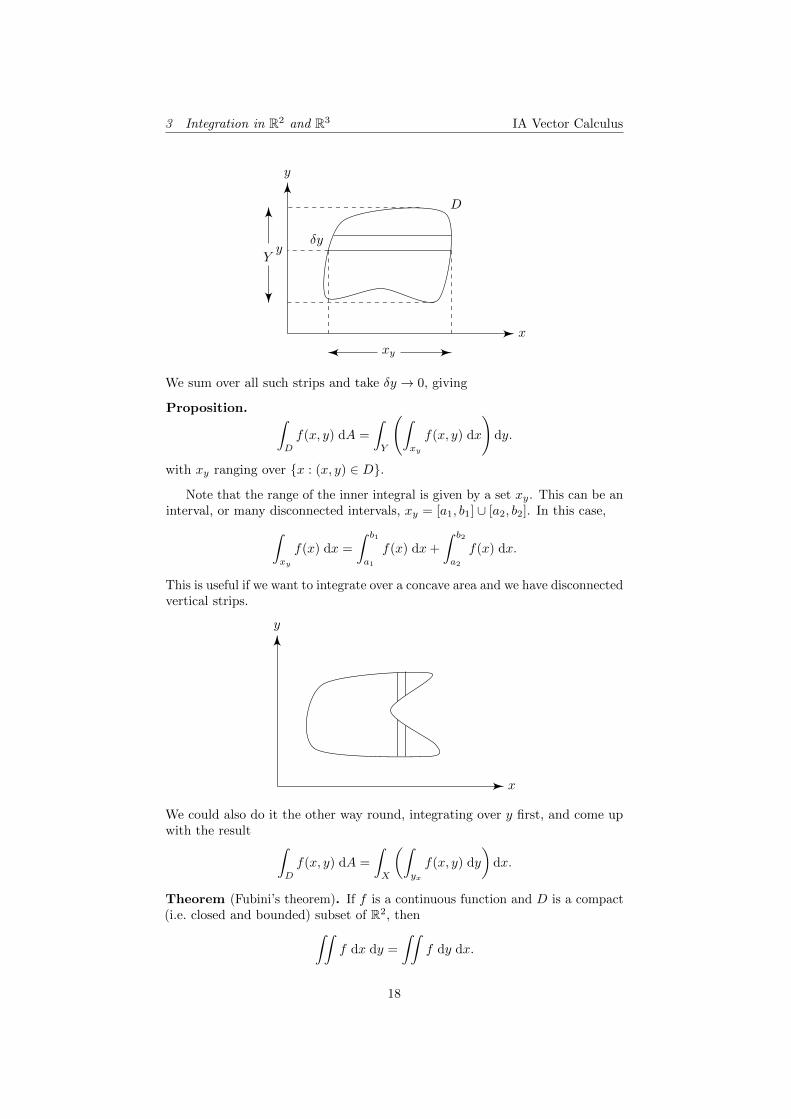
3 Integration in R2 and R3 IA Vector Calculus
x
y
δyy
xy
Y
D
We sum over all such strips and take δy → 0, giving
Proposition. ∫D
f(x, y) dA =
∫Y
(∫xy
f(x, y) dx
)dy.
with xy ranging over {x : (x, y) ∈ D}.
Note that the range of the inner integral is given by a set xy. This can be aninterval, or many disconnected intervals, xy = [a1, b1] ∪ [a2, b2]. In this case,∫
xy
f(x) dx =
∫ b1
a1
f(x) dx+
∫ b2
a2
f(x) dx.
This is useful if we want to integrate over a concave area and we have disconnectedvertical strips.
x
y
We could also do it the other way round, integrating over y first, and come upwith the result ∫
D
f(x, y) dA =
∫X
(∫yx
f(x, y) dy
)dx.
Theorem (Fubini’s theorem). If f is a continuous function and D is a compact(i.e. closed and bounded) subset of R2, then∫∫
f dx dy =
∫∫f dy dx.
18

3 Integration in R2 and R3 IA Vector Calculus
While we have rather strict conditions for this theorem, it actually holds in manymore cases, but those situations have to be checked manually.
Definition (Area element). The area element is dA.
Proposition. dA = dx dy in Cartesian coordinates.
Example. We integrate over the triangle bounded by (0, 0), (2, 0) and (0, 1).We want to integrate the function f(x, y) = x2y over the area. So∫
D
f(xy) dA =
∫ 1
0
(∫ 2−2y
0
x2y dx
)dy
=
∫ 1
0
y
[x3
3
]2−2y
0
dy
=8
3
∫ 1
0
y(1− y)3 dy
=2
15
We can integrate it the other way round:∫D
x2y dA =
∫ 2
0
∫ 1−x/2
0
x2y dy dx
=
∫ 2
0
x2
[1
2y2
]1−x/2
0
dx
=
∫ 2
0
x2
2
(1− x
2
)2
dx
=2
15
Since it doesn’t matter whether we integrate x first or y first, if we find itdifficult to integrate one way, we can try doing it the other way and see if it iseasier.
While this integral is tedious in general, there is a special case where it issubstantially easier.
Definition (Separable function). A function f(x, y) is separable if it can bewritten as f(x, y) = h(y)g(x).
Proposition. Take separable f(x, y) = h(y)g(x) and D be a rectangle {(x, y) :a ≤ x ≤ b, c ≤ y ≤ d}. Then∫
D
f(x, y) dx dy =
(∫ b
a
g(x) dx
)(∫ d
c
h(y) dy
)
3.2 Change of variables for an integral in R2
Proposition. Suppose we have a change of variables (x, y) ↔ (u, v) that issmooth and invertible, with regions D,D′ in one-to-one correspondence. Then∫
D
f(x, y) dx dy =
∫D
f(x(u, v), y(u, v))|J | du dv,
19

3 Integration in R2 and R3 IA Vector Calculus
where
J =∂(x, y)
∂(u, v)=
∣∣∣∣∣∣∣∂x
∂u
∂x
∂v∂y
∂u
∂y
∂v
∣∣∣∣∣∣∣is the Jacobian. In other words,
dx dy = |J | du dv.
Proof. Since we are writing (x(u, v), y(u, v)), we are actually transforming from(u, v) to (x, y) and not the other way round.
Suppose we start with an area δA′ = δuδv in the (u, v) plane. Then byTaylors’ theorem, we have
δx = x(u+ δu, v + δv)− x(u, v) ≈ ∂x
∂uδu+
∂x
∂vδv.
We have a similar expression for δy and we obtain(δxδy
)≈(∂x∂u
∂x∂v
∂y∂u
∂y∂v
)(δuδv
)Recall from Vectors and Matrices that the determinant of the matrix is howmuch it scales up an area. So the area formed by δx and δy is |J | times the areaformed by δu and δv. Hence
dx dy = |J | du dv.
Example. We transform from (x, y) to (ρ, ϕ) with
x = ρ cosϕ
y = ρ sinϕ
We have previously calculated that |J | = ρ. So
dA = ρ dρ dϕ.
Suppose we want to integrate a function over a quarter area D of radius R.
x
y
D
Let the function to be integrated be f = exp(−(x2 +y2)/2) = exp(−ρ2/2). Then∫f dA =
∫fρ dρ dϕ
=
∫ R
ρ=0
(∫ π/2
ϕ=0
e−ρ2/2ρ dϕ
)δρ
20

3 Integration in R2 and R3 IA Vector Calculus
Note that in polar coordinates, we are integrating over a rectangle and thefunction is separable. So this is equal to
=[−e−ρ
2/2]R
0[ϕ]
π/20
=π
2
(1− e−R
2/2). (∗)
Note that the integral exists as R→∞.Now we take the case of x, y →∞ and consider the original integral.∫
D
f dA =
∫ ∞x=0
∫ ∞y=0
e−(x2+y2)/2 dx dy
=
(∫ ∞0
e−x2/2 dx
)(∫ ∞0
e−y2/2 dy
)=π
2
where the last line is from (*). So each of the two integrals must be√π/2, i.e.∫ ∞
0
e−x2/2 dx =
√π
2.
3.3 Generalization to R3
We will do exactly the same thing as we just did, but with one more dimension:
Definition (Volume integral). Consider a volume V ⊆ R3 with position vectorr = (x, y, z). We approximate V by N small disjoint subsets of some simpleshape (e.g. cuboids) labelled by I, volume δVI , contained within a solid sphereof diameter `.
Assume that as `→ 0 and N →∞, the union of the small subsets tend toV . Then ∫
V
f(r) dV = lim`→0
∑I
f(r∗I)δVI ,
where r∗I is any chosen point in each small subset.
To evaluate this, we can take δVI = δxδyδz, and take δx→ 0, δy → 0 andδz in some order. For example,∫
V
f(r) dv =
∫D
(∫Zxy
f(x, y, z) dz
)dx dy.
So we integrate f(x, y, z) over z at each point (x, y), then take the integral ofthat over the area containing all required (x, y).
Alternatively, we can take the area integral first, and have∫V
f(r) dV =
∫z
(∫DZ
f(x, y, z) dx dy
)dz.
Again, if we take f = 1, then we obtain the volume of V .Often, f(r) is the density of some quantity, and is usually denoted by ρ. For
example, we might have mass density, charge density, or probability density.ρ(r)δV is then the amount of quantity in a small volume δV at r. Then∫Vρ(r) dV is the total amount of quantity in V .
21

3 Integration in R2 and R3 IA Vector Calculus
Definition (Volume element). The volume element is dV .
Proposition. dV = dx dy dz.
We can change variables by some smooth, invertible transformation (x, y, z) 7→(u, v, w). Then
Proposition. ∫V
f dx dy dz =
∫V
f |J | du dv dw,
with
J =∂(x, y, z)
∂(u, v, w)=
∣∣∣∣∣∣∣∣∣∣∣∣
∂x
∂u
∂x
∂v
∂x
∂w∂y
∂u
∂y
∂v
∂y
∂w∂z
∂u
∂z
∂v
∂z
∂w
∣∣∣∣∣∣∣∣∣∣∣∣Proposition. In cylindrical coordinates,
dV = ρ dρ dϕ dz.
In spherical coordinates
dV = r2 sin θ dr dθ dϕ.
Proof. Loads of algebra.
Example. Suppose f(r) is spherically symmetric and V is a sphere of radius acentered on the origin. Then∫
V
f dV =
∫ a
r=0
∫ π
θ=0
∫ 2π
ϕ=0
f(r)r2 sin θ dr dθ dϕ
=
∫ a
0
dr
∫ π
0
dθ
∫ 2π
0
dϕ r2f(r) sin θ
=
∫ a
0
r2f(r)dr[− cos θ
]π0
[ϕ]2π
0
= 4π
∫ a
0
f(r)r2 dr.
where we separated the integral into three parts as in the area integrals.Note that in the second line, we rewrote the integrals to write the differentials
next to the integral sign. This is simply a different notation that saves us fromwriting r = 0 etc. in the limits of the integrals.
This is a useful general result. We understand it as the sum of sphericalshells of thickness δr and volume 4πr2δr.
If we take f = 1, then we have the familiar result that the volume of a sphereis 4
3πa3.
Example. Consider a volume within a sphere of radius a with a cylinder ofradius b (b < a) removed. The region is defined as
x2 + y2 + z2 ≤ a2
x2 + y2 ≥ b2.
22

3 Integration in R2 and R3 IA Vector Calculus
a
b
We use cylindrical coordinates. The second criteria gives
b ≤ ρ ≤ a.
For the x2 + y2 + z2 ≤ a2 criterion, we have
−√a2 − ρ2 ≤ z ≤
√a2 − ρ2.
So the volume is ∫V
dV =
∫ a
b
dρ
∫ 2π
0
dϕ
∫ √a2−ρ2−√a2−ρ2
dz ρ
= 2π
∫ a
b
2ρ√a2 − ρ2 dρ
= 2π
[2
3(a2 − ρ2)3/2
]ab
=4
3π(a2 − b2)3/2.
Example. Suppose the density of electric charge ρ(r) = ρ0za in a hemisphere
H of radius a, with z ≥ 0. What is the total charge of H?We use spherical polars. So
r ≤ a, 0 ≤ ϕ ≤ 2π, 0 ≤ θ ≤ π
2.
We haveρ(r) =
ρ0
ar cos θ.
The total charge Q in H is∫H
ρ dV =
∫ a
0
dr
∫ π/2
0
dθ
∫ 2π
0
dϕρ0
ar cos θr2 sin θ
=ρ0
a
∫ a
0
r3 dr
∫ π/2
0
sin θ cos θ dθ
∫ 2π
0
dϕ
=ρ0
a
[r4
4
]a0
[1
2sin2 θ
]π/20
[ϕ]2π0
=ρ0πa
3
4.
23

3 Integration in R2 and R3 IA Vector Calculus
3.4 Further generalizations
Integration in Rn
Similar to the above,∫Df(x1, x2, · · ·xn) dx1 dx2 · · · dxn is simply the integra-
tion over an n-dimensional volume. The change of variable formula is
Proposition.∫D
f(x1, x2, · · ·xn) dx1 dx2 · · · dxn =
∫D′f({xi(u)})|J | du1 du2 · · · dun.
Change of variables for n = 1
In the n = 1 case, the Jacobian is dxdu . However, we use the following formula for
change of variables: ∫D
f(x) dx =
∫D′f(x(u))
∣∣∣∣dxdu
∣∣∣∣ du.
We introduce the modulus because of our natural convention about integrating
over D and D′. If D = [a, b] with a < b, we write∫ ba
. But if a 7→ α and b 7→ β,
but α > β, we would like to write∫ αβ
instead, so we introduce the modulus inthe 1D case.
To show that the modulus is the right thing to do, we check case by case: Ifa < b and α < β, then dx
du is positive, and we have, as expected∫ b
a
f(x) dx =
∫ β
α
f(u)dx
dudu.
If α > β, then dxdu is negative. So∫ b
a
f(x) dx =
∫ β
α
f(u)dx
dudu = −
∫ α
β
f(u)dx
dudu.
By taking the absolute value of dxdu , we ensure that we always have the numerically
smaller bound as the lower bound.This is not easily generalized to higher dimensions, so we don’t employ the
same trick in other cases.
Vector-valued integrals
We can define∫V
F(r) dV in a similar way to∫Vf(r) dV as the limit of a sum over
small contributions of volume. In practice, we integrate them componentwise. If
F(r) = Fi(r)ei,
then ∫V
F(r) dV =
∫V
(Fi(r) dV )ei.
For example, if a mass has density ρ(r), then its mass is
M =
∫V
ρ(r) dV
24

3 Integration in R2 and R3 IA Vector Calculus
and its center of mass is
R =1
M
∫V
rρ(r) dV.
Example. Consider a solid hemisphere H with r ≤ a, z ≥ 0 with uniformdensity ρ. The mass is
M =
∫H
ρ dV =2
3πa3ρ.
Now suppose that R = (X,Y, Z). By symmetry, we expect X = Y = 0. We canfind this formally by
X =1
M
∫H
xρ dV
=ρ
M
∫ a
0
∫ π/2
0
∫ 2π
0
xr2 sin θ dϕ dθ dr
=ρ
M
∫ a
0
r3 dr ×∫ π/2
0
sin2 θ dθ ×∫ 2π
0
cosϕ dϕ
= 0
as expected. Note that it evaluates to 0 because the integral of cos from 0 to 2πis 0. Similarly, we obtain Y = 0.
Finally, we find Z.
Z =ρ
M
∫ a
0
r3 dr
∫ π/2
0
sin θ cos θ dθ
∫ 2π
0
dϕ
=r
M
[a4
4
] [1
2sin2 θ
]π/20
2π
=3a
8.
So R = (0, 0, 3a/8).
25

4 Surfaces and surface integrals IA Vector Calculus
4 Surfaces and surface integrals
4.1 Surfaces and Normal
So far, we have learnt how to do calculus with regions of the plane or space.What we would like to do now is to study surfaces in R3. The first thing tofigure out is how to specify surfaces. One way to specify a surface is to use anequation. We let f be a smooth function on R3, and c be a constant. Thenf(r) = c defines a smooth surface (e.g. x2 + y2 + z2 = 1 denotes the unit sphere).
Now consider any curve r(u) on S. Then by the chain rule, if we differentiatef(r) = c with respect to u, we obtain
d
du[f(r(u))] = ∇f · dr
du= 0.
This means that ∇f is always perpendicular to drdu . Since dr
du is the tangent tothe curve, ∇f is perpendicular to the tangent. Since this is true for any curver(u), ∇f is perpendicular to any tangent of the surface. Therefore
Proposition. ∇f is the normal to the surface f(r) = c.
Example.
(i) Take the sphere f(r) = x2 + y2 + z2 = c for c > 0. Then ∇f = 2(x, y, z) =2r, which is clearly normal to the sphere.
(ii) Take f(r) = x2 + y2 − z2 = c, which is a hyperboloid. Then ∇f =2(x, y,−z).In the special case where c = 0, we have a double cone, with a singular apex0. Here ∇f = 0, and we cannot find a meaningful direction of normal.
Definition (Boundary). A surface S can be defined to have a boundary ∂Sconsisting of a piecewise smooth curve. If we define S as in the above examplesbut with the additional restriction z ≥ 0, then ∂S is the circle x2 + y2 = c, z = 0.
A surface is bounded if it can be contained in a solid sphere, unboundedotherwise. A bounded surface with no boundary is called closed (e.g. sphere).
Example.
The boundary of a hemisphere is a circle (drawn in red).
Definition (Orientable surface). At each point, there is a unit normal n that’sunique up to a sign.
If we can find a consistent choice of n that varies smoothly across S, thenwe say S is orientable, and the choice of sign of n is called the orientation of thesurface.
26

4 Surfaces and surface integrals IA Vector Calculus
Most surfaces we encounter are orientable. For example, for a sphere, we candeclare that the normal should always point outwards. A notable example of anon-orientable surface is the Mobius strip (or Klein bottle).
For simple cases, we can describe the orientation as “inward” and “outward”.
4.2 Parametrized surfaces and area
However, specifying a surface by an equation f(r) = c is often not too helpful.What we would like is to put some coordinate system onto the surface, so thatwe can label each point by a pair of numbers (u, v), just like how we label pointsin the x, y-plane by (x, y). We write r(u, v) for the point labelled by (u, v).
Example. Let S be part of a sphere of radius a with 0 ≤ θ ≤ α.
α
We can then label the points on the spheres by the angles θ, ϕ, with
r(θ, ϕ) = (a cosϕ sin θ, a sin θ sinϕ, a cos θ) = aer.
We restrict the values of θ, ϕ by 0 ≤ θ ≤ α, 0 ≤ ϕ ≤ 2π, so that each point isonly covered once.
Note that to specify a surface, in addition to the function r, we also haveto specify what values of (u, v) we are allowed to take. This corresponds to aregion D of allowed values of u and v. When we do integrals with these surfaces,these will become the bounds of integration.
When we have such a parametrization r, we would want to make sure thisindeed gives us a two-dimensional surface. For example, the following twoparametrizations would both be bad:
r(u, v) = u, r(u, v) = u+ v.
The idea is that r has to depend on both u and v, and in “different ways”.More precisely, when we vary the coordinates (u, v), the point r will changeaccordingly. By the chain rule, this is given by
δr =∂r
∂uδu+
∂r
∂vδv + o(δu, δv).
Then ∂rδu and ∂r
∂v are tangent vectors to curves on S with v and u constantrespectively. What we want is for them to point in different directions.
Definition (Regular parametrization). A parametrization is regular if for allu, v,
∂r
∂u× ∂r
∂v6= 0,
i.e. there are always two independent tangent directions.
27

4 Surfaces and surface integrals IA Vector Calculus
The parametrizations we use will all be regular.Given a surface, how could we, say, find its area? We can use our parametriza-
tion. Suppose points on the surface are given by r(u, v) for (u, v) ∈ D. If wewant to find the area of D itself, we would simply integrate∫
D
du dv.
However, we are just using u and v as arbitrary labels for points in the surface,and one unit of area in D does not correspond to one unit of area in S. Instead,suppose we produce a small rectangle in D by changing u and v by small δu, δv.In D, this corresponds to a rectangle with vertices (u, v), (u + δu, v), (u, v +δv), (u + δu, v + δv), and spans an area δuδv. In the surface S, these smallchanges δu, δv correspond to changes ∂r
∂uδu and ∂r∂v δv, and these span a vector
area of
δS =∂r
∂u× ∂r
∂vδuδv = n δS.
Note that the order of u, v gives the choice of the sign of the unit normal.The actual area is then given by
δS =
∣∣∣∣ ∂r
∂u× ∂r
∂v
∣∣∣∣ δu δv.Making these into differentials instead of deltas, we have
Proposition. The vector area element is
dS =∂r
∂u× ∂r
∂vdu dv.
The scalar area element is
dS =
∣∣∣∣ ∂r
∂u× ∂r
∂v
∣∣∣∣ du dv.
By summing and taking limits, the area of S is∫S
dS =
∫D
∣∣∣∣ ∂r
∂u× ∂r
∂v
∣∣∣∣du dv.
Example. Consider again the part of the sphere of radius a with 0 ≤ θ ≤ α.
α
Then we have
r(θ, ϕ) = (a cosϕ sin θ, a sin θ sinϕ, a cos θ) = aer.
So we find∂r
∂θ= aeθ.
28

4 Surfaces and surface integrals IA Vector Calculus
Similarly, we have∂r
∂ϕ= a sin θeϕ.
Then∂r
∂θ× ∂r
∂ϕ= a2 sin θ er.
SodS = a2 sin θ dθ dϕ.
Our bounds are 0 ≤ θ ≤ α, 0 ≤ ϕ ≤ 2π.Then the area is∫ 2π
0
∫ α
0
a2 sin θ dθ dϕ = 2πa2(1− cosα).
4.3 Surface integral of vector fields
Just computing the area of a surface would be boring. Suppose we have a surfaceS parametrized by r(u, v), where (u, v) takes values in D. We would like to askhow much “stuff” is passing through S, where the flow of stuff is given by avector field F(r).
We might attempt to use the integral∫D
|F| dS.
However, this doesn’t work. For example, if all the flow is tangential to thesurface, then nothing is really passing through the surface, but |F| is non-zero,so we get a non-zero integral. Instead, what we should do is to consider thecomponent of F that is normal to the surface S, i.e. parallel to its normal.
Definition (Surface integral). The surface integral or flux of a vector field F(r)over S is defined by∫
S
F(r) · dS =
∫S
F(r) · n dS =
∫D
F(r(u, v)) ·(∂r
∂u× ∂r
∂v
)du dv.
Intuitively, this is the total amount of F passing through S. For example, ifF is the electric field, the flux is the amount of electric field passing through asurface.
For a given orientation, the integral∫
F·dS is independent of the parametriza-tion. Changing orientation is equivalent to changing the sign of n, which is inturn equivalent to changing the order of u and v in the definition of S, which isalso equivalent to changing the sign of the flux integral.
Example. Consider a sphere of radius a, r(θ, ϕ). Then
∂r
∂θ= aeθ,
∂r
∂ϕ= a sin θeϕ.
The vector area element is
dS = a2 sin θer dθ dϕ,
29

4 Surfaces and surface integrals IA Vector Calculus
taking the outward normal n = er = r/a.Suppose we want to calculate the fluid flux through the surface. The velocity
field u(r) of a fluid gives the motion of a small volume of fluid r. Assume thatu depends smoothly on r (and t). For any small area δS, on a surface S, thevolume of fluid crossing it in time δt is u · δS δt.
δS
u δt
n
So the amount of flow of u over at time δt through S is
δt
∫S
u · dS.
So∫S
u · dS is the rate of volume crossing S.For example, let u = (−x, 0, z) and S be the section of a sphere of radius a
with 0 ≤ ϕ ≤ and 0 ≤ θ ≤ α. Then
dS = a2 sin θn dϕ dθ,
with
n =r
a=
1
a(x, y, z).
So
n · u =1
a(−x2 + z2) = a(− sin2 θ cos2 ϕ+ cos2 θ).
Therefore∫S
u · dS =
∫ α
0
∫ 2π
0
a3 sin θ[(cos2 θ − 1) cos2 ϕ+ cos2 θ] dϕ dθ
=
∫ α
0
a3 sin θ[π(cos2θ − 1) + 2π cos2 θ] dθ
=
∫ α
0
a3π(3 cos3 θ − 1) sin θ dθ
= πa3[cosθ − cos3 θ]α0
= πa3 cosα sin2 α.
What happens when we change parametrization? Let r(u, v) and r(u, v) betwo regular parametrizations for the surface. By the chain rule,
∂r
∂u=∂r
∂u
∂u
∂u+∂r
∂v
∂v
∂u∂r
∂v=∂r
∂u
∂u
∂v+∂r
∂v
∂v
∂v
So∂r
∂u× ∂r
∂v=∂(u, v)
∂(u, v)
∂r
∂u× ∂r
∂v
30

4 Surfaces and surface integrals IA Vector Calculus
where ∂(u,v)∂(u,v) is the Jacobian.
Since
du dv =∂(u, v)
∂(u, v)du dv,
We recover the formula
dS =
∣∣∣∣ ∂r
∂u× ∂r
∂v
∣∣∣∣ du dv =
∣∣∣∣ ∂r
∂u× ∂r
∂v
∣∣∣∣ du dv.
Similarly, we have
dS =∂r
∂u× ∂r
∂vdu dv =
∂r
∂u× ∂r
∂vdu dv.
provided (u, v) and (u, v) have the same orientation.
4.4 Change of variables in R2 and R3 revisited
In this section, we derive our change of variable formulae in a slightly differentway.
Change of variable formula in R2
We first derive the 2D change of variable formula from the 3D surface integralformula.
Consider a subset S of the plane R2 parametrized by r(x(u, v), y(u, v)). Wecan embed it to R3 as r(x(u, v), y(u, v), 0). Then
∂r
∂u× ∂r
∂v= (0, 0, J),
with J being the Jacobian. Therefore∫S
f(r) dS =
∫D
f(r(u, v))
∣∣∣∣ ∂r
∂u× ∂r
∂v
∣∣∣∣ du dv =
∫D
f(r(u, v))|J | du dv,
and we recover the formula for changing variables in R2.
Change of variable formula in R3
In R3, suppose we have a volume parametrised by r(u, v, w). Then
δr =∂r
∂uδu+
∂r
∂vδv +
∂r
∂wδw + o(δu, δv, δw).
Then the cuboid δu, δv, δw in u, v, w space is mapped to a parallelopiped ofvolume
δV =
∣∣∣∣ ∂r
∂uδu ·
(∂r
∂vδv × ∂r
∂wδw
)∣∣∣∣ = |J | δu δv δw.
So dV = |J | du dv dw.
31

5 Geometry of curves and surfaces IA Vector Calculus
5 Geometry of curves and surfaces
Let r(s) be a curve parametrized by arclength s. Since t(s) = drds is a unit vector,
t · t = 1. Differentiating yields t · t′ = 0. So t′ is a normal to the curve if t′ 6= 0.We define the following:
Definition (Principal normal and curvature). Write t′ = κn, where n is a unitvector and κ > 0. Then n(s) is called the principal normal and κ(s) is calledthe curvature.
Note that we must be differentiating against s, not any other parametrization!If the curve is given in another parametrization, we can either change theparametrization or use the chain rule.
We take a curve that can Taylor expanded around s = 0. Then
r(s) = r(0) + sr′(0) +1
2s2r′′(0) +O(s3).
We know that r′ = t and r′′ = t′. So we have
r(s) = r(0) + st(0) +1
2κ(0)s2n +O(s3).
How can we interpret κ as the curvature? Suppose we want to approximate thecurve near r(0) by a circle. We would expect a more “curved” curve would beapproximated by a circle of smaller radius. So κ should be inversely proportionalto the radius of the circle. In fact, we will show that κ = 1/a, where a is theradius of the best-fit circle.
Consider the vector equation for a circle passing through r(0) with radius ain the plane defined by t and n.
a
r(0)t
n θ
Then the equation of the circle is
r = r(0) + a(1− cos θ)n + a sin θt.
We can expand this to obtain
r = r(0) + aθt +1
2θ2an + o(θ3).
Since the arclength s = aθ, we obtain
r = r(0) + st +1
2
1
as2n +O(s3).
As promised, κ = 1/a, for a the radius of the circle of best fit.
32

5 Geometry of curves and surfaces IA Vector Calculus
Definition (Radius of curvature). The radius of curvature of a curve at a pointr(s) is 1/κ(s).
Since we are in 3D, given t(s) and n(s), there is another normal to the curve.We can add a third normal to generate an orthonormal basis.
Definition (Binormal). The binormal of a curve is b = t× n.
We can define the torsion similar to the curvature, but with the binormalinstead of the tangent.1
Definition (Torsion). Let b′ = −τn. Then τ is the torsion.
Note that this makes sense, since b′ is both perpendicular to t and b, andhence must be in the same direction as n. (b′ = t′ × n + t× n′ = t× n′, so b′
is perpendicular to t; and b · b = 1⇒ b · b′ = 0. So b′ is perpendicular to b).The geometry of the curve is encoded in how this basis (t,n,b) changes along
it. This can be specified by two scalar functions of arc length — the curvatureκ(s) and the torsion τ(s) (which determines what the curve looks like to thirdorder in its Taylor expansions and how the curve lifts out of the t, r plane).
Surfaces and intrinsic geometry*
We can study the geometry of surfaces through curves which lie on them. At agiven point P at a surface S with normal n, consider a plane containing n. Theintersection of the plane with the surface yields a curve on the surface throughP . This curve has a curvature κ at P .
If we choose different planes containing n, we end up with different curves ofdifferent curvature. Then we define the following:
Definition (Principal curvature). The principal curvatures of a surface at P arethe minimum and maximum possible curvature of a curve through P , denotedκmin and κmax respectively.
Definition (Gaussian curvature). The Gaussian curvature of a surface at apoint P is K = κminκmax.
Theorem (Theorema Egregium). K is intrinsic to the surface S. It can beexpressed in terms of lengths, angles etc. which are measured entirely on thesurface. So K can be defined on an arbitrary surface without embedding it on ahigher dimension surface.
The is the start of intrinsic geometry : if we embed a surface in Euclideanspace, we can determine lengths, angles etc on it. But we don’t have to do so —we can “live in ” the surface and do geometry in it without an embedding.
For example, we can consider a geodesic triangle D on a surface S. It consistsof three geodesics: shortest curves between two points.
Let θi be the interior angles of the triangle (defined by using scalar productsof tangent vectors). Then
1This was not taught in lectures, but there is a question on the example sheet about thetorsion, so I might as well include it here.
33

5 Geometry of curves and surfaces IA Vector Calculus
Theorem (Gauss-Bonnet theorem).
θ1 + θ2 + θ3 = π +
∫D
K dA,
integrating over the area of the triangle.
34

6 Div, Grad, Curl and ∇ IA Vector Calculus
6 Div, Grad, Curl and ∇6.1 Div, Grad, Curl and ∇Recalled that ∇f is given by (∇f)i = ∂f
∂xi. We can regard this as obtained from
the scalar field f by applying
∇ = ei∂
∂xi
for cartesian coordinates xi and orthonormal basis ei, where ei are orthonormaland right-handed, i.e. ei × ej = εijkek (it is left handed if ei × ej = −εijkek).
We can alternatively write this as
∇ =
(∂
∂x,∂
∂y,∂
∂z
).
∇ (nabla or del) is both an operator and a vector. We can apply it to a vectorfield F(r) = Fi(r)ei using the scalar or vector product.
Definition (Divergence). The divergence or div of F is
∇ · F =∂Fi∂xi
=∂F1
∂x1+∂F2
∂x2+∂F3
∂x3.
Definition (Curl). The curl of F is
∇× F = εijk∂Fk∂xj
ei =
∣∣∣∣∣∣e1 e2 e3∂∂x
∂∂y
∂∂z
Fx Fy Fz
∣∣∣∣∣∣Example. Let F = (xez, y2 sinx, xyz). Then
∇ · F =∂
∂xxez +
∂
∂yy2 sinx+
∂
∂zxyz = ez + 2y sinx+ xy.
and
∇× F = i
[∂
∂y(xyz)− ∂
∂z(y2 sinx)
]+ j
[∂
∂z(xez) +
∂
∂x(xyz)
]+ k
[∂
∂x(y2 sinx)− ∂
∂y(xez)
]= (xz, xez − yz, y2 cosx).
Note that ∇ is an operator, so ordering is important. For example,
F · ∇ = Fi∂
∂xi
is a scalar differential operator, and
F×∇ = ekεijkFi∂
∂xj
is a vector differential operator.
35

6 Div, Grad, Curl and ∇ IA Vector Calculus
Proposition. Let f, g be scalar functions, F,G be vector functions, and µ, λbe constants. Then
∇(λf + µg) = λ∇f + µ∇g∇ · (λF + µG) = λ∇ · F + µ∇ ·G∇× (λF + µG) = λ∇× F + µ∇×G.
Note that Grad and Div can be analogously defined in any dimension n, butcurl is specific to n = 3 because it uses the vector product.
Example. Consider rα with r = |r|. We know that r = xiei. So r2 = xixi.Therefore
2r∂r
∂xj= 2xj ,
or∂r
∂xi=xir.
So
∇rα = ei∂
∂xi(rα) = eiαr
α−1 ∂r
∂xi= αrα−2r.
Also,
∇ · r =∂xi∂xi
= 3.
and
∇× r = ekεijk∂xj∂xi
= 0.
Proposition. We have the following Leibnitz properties:
∇(fg) = (∇f)g + f(∇g)
∇ · (fF) = (∇f) · F + f(∇ · F)
∇× (fF) = (∇f)× F + f(∇× F)
∇(F ·G) = F× (∇×G) + G× (∇× F) + (F · ∇)G + (G · ∇)F
∇× (F×G) = F(∇ ·G)−G(∇ · F) + (G · ∇)F− (F · ∇)G
∇ · (F×G) = (∇× F) ·G− F · (∇×G)
which can be proven by brute-forcing with suffix notation and summationconvention.
There is absolutely no point in memorizing these (at least the last three).They can be derived when needed via suffix notation.
Example.
∇ · (rαr) = (∇rα)r + rα∇ · r= (αrα−2r) · r + rα(3)
= (α+ 3)rα
∇× (rαr) = (∇(rα))× r + rα(∇× r)
= αrα−2r× r
= 0
36

6 Div, Grad, Curl and ∇ IA Vector Calculus
6.2 Second-order derivatives
We have
Proposition.
∇× (∇f) = 0
∇ · (∇× F) = 0
Proof. Expand out using suffix notation, noting that
εijk∂2f
∂xi∂xj= 0.
since if, say, k = 3, then
εijk∂2f
∂xi∂xj=
∂2f
∂x1∂x2− ∂2f
∂x2∂x1= 0.
The converse of each result holds for fields defined in all of R3:
Proposition. If F is defined in all of R3, then
∇× F = 0⇒ F = ∇f
for some f .
Definition (Conservative/irrotational field and scalar potential). If F = ∇f ,then f is the scalar potential. We say F is conservative or irrotational.
Similarly,
Proposition. If H is defined over all of R3 and ∇ ·H = 0, then H = ∇×Afor some A.
Definition (Solenoidal field and vector potential). If H = ∇ × A, A is thevector potential and H is said to be solenoidal.
Not that is is true only if F or H is defined on all of R3.
Definition (Laplacian operator). The Laplacian operator is defined by
∇2 = ∇ · ∇ =∂2
∂xi∂xi=
(∂2
∂x21
+∂2
∂x22
+∂2
∂x33
).
This operation is defined on both scalar and vector fields — on a scalar field,
∇2f = ∇ · (∇f),
whereas on a vector field,
∇2A = ∇(∇ ·A)−∇× (∇×A).
37

7 Integral theorems IA Vector Calculus
7 Integral theorems
7.1 Statement and examples
There are three big integral theorems, known as Green’s theorem, Stoke’s theoremand Gauss’ theorem. There are all generalizations of the fundamental theorem ofcalculus in some sense. In particular, they all say that an n dimensional integralof a derivative is equivalent to an n − 1 dimensional integral of the originalfunction.
We will first state all three theorems with some simple applications. In thenext section, we will see that the three integral theorems are so closely relatedthat it’s easiest to show their equivalence first, and then prove just one of them.
7.1.1 Green’s theorem (in the plane)
Theorem (Green’s theorem). For smooth functions P (x, y), Q(x, y) and A abounded region in the (x, y) plane with boundary ∂A,∫
A
(∂Q
∂x− ∂P
∂y
)dA =
∫∂A
(P dx+Q dy).
Given that C is a piecewise smooth, non-intersecting closed curve, traversedanti-clockwise.
Example. Let Q = xy2 and P = x2y. If C is the parabola y2 = 4ax and theline x = a, both with −2a ≤ y ≤ 2a, then Green’s theorem says∫
A
(y2 − x2) dA =
∫C
x2 dx+ xy2 dy.
From example sheet 1, each side gives 104105a
4.
Example. Let A be a rectangle confined by 0 ≤ x ≤ a and 0 ≤ y ≤ b.
x
y
a
b
A
Then Green’s theorem follows directly form the fundamental theorem of calculusin 1D. We first consider the first term of Green’s theorem:∫
−∂P∂y
dA =
∫ a
0
∫ b
0
−∂P∂y
dy dx
=
∫ a
0
[−P (x, b) + P (x, 0)] dx
=
∫C
P dx
38

7 Integral theorems IA Vector Calculus
Note that we can convert the 1D integral in the second-to-last line to a line integralaround the curve C, since the P (x, 0) and P (x, b) terms give the horizontal partof C, and the lack of dy term means that the integral is nil when integrating thevertical parts.
Similarly, ∫A
∂Q
∂xdA =
∫C
Q dy.
Combining them gives Green’s theorem.
Green’s theorem also holds for a bounded region A, where the boundary ∂Aconsists of disconnected components (each piecewise smooth, non-intersectingand closed) with anti-clockwise orientation on the exterior, and clockwise on theinterior boundary, e.g.
The orientation of the curve comes from imagining the surface as:
and take the limit as the gap shrinks to 0.
7.1.2 Stokes’ theorem
Theorem (Stokes’ theorem). For a smooth vector field F(r),∫S
∇× F · dS =
∫∂S
F · dr,
where S is a smooth, bounded surface and ∂S is a piecewise smooth boundaryof S.
The direction of the line integral is as follows: If we walk along C with nfacing up, then the surface is on your left.
It also holds if ∂S is a collection of disconnected piecewise smooth closedcurves, with the orientation determined in the same way as Green’s theorem.
39

7 Integral theorems IA Vector Calculus
Example. Let S be the section of a sphere of radius a with 0 ≤ θ ≤ α. Inspherical coordinates,
dS = a2 sin θer dθ dϕ.
Let F = (0, xz, 0). Then ∇× F = (−x, 0, z). We have previously shown that∫S
∇× F · dS = πa3 cosα sin2 α.
Our boundary ∂C is
r(ϕ) = a(sinα cosϕ, sinα sinϕ, cosα).
The right hand side of Stokes’ is∫C
F · dr =
∫ 2π
0
a sinα cosϕ︸ ︷︷ ︸x
a cosα︸ ︷︷ ︸z
a sinα cosϕ dϕ︸ ︷︷ ︸dy
= a3 sin2 α cosα
∫ 2π
0
cos2 ϕ dϕ
= πa3 sin2 α cosα.
So they agree.
7.1.3 Divergence/Gauss theorem
Theorem (Divergence/Gauss theorem). For a smooth vector field F(r),∫V
∇ · F dV =
∫∂V
F · dS,
where V is a bounded volume with boundary ∂V , a piecewise smooth, closedsurface, with outward normal n.
Example. Consider a hemisphere.
S2
S1
V is a solid hemisphere
x2 + y2 + z2 ≤ a2, z ≥ 0,
and ∂V = S1 + S2, the hemisphere and the disc at the bottom.Take F = (0, 0, z + a) and ∇ · F = 1. Then∫
V
∇ · F dV =2
3πa3,
the volume of the hemisphere.
40

7 Integral theorems IA Vector Calculus
On S1,
dS = n dS =1
a(x, y, z) dS.
Then
F · dS =1
az(z + a) dS = cos θa(cos θ + 1) a2 sin θ dθ dϕ︸ ︷︷ ︸
dS
.
Then ∫S1
F · dS = a3
∫ 2π
0
dϕ
∫ π/2
0
sin θ(cos2 θ + cos θ) dθ
= 2πa3
[−1
3cos3 θ − 1
2cos2 θ
]π/20
=5
3πa3.
On S2, dS = n dS = −(0, 0, 1) dS. Then F · dS = −a dS. So∫S2
F · dS = −πa3.
So ∫S1
F · dS +
∫S2
F · dS =
(5
3− 1
)πa3 =
2
3πa3,
in accordance with Gauss’ theorem.
7.2 Relating and proving integral theorems
We will first show the following two equivalences:
– Stokes’ theorem ⇔ Green’s theorem
– 2D divergence theorem ⇔ Greens’ theorem
Then we prove the 2D version of divergence theorem directly to show that all ofthe above hold. A sketch of the proof of the 3D version of divergence theoremwill be provided, because it is simply a generalization of the 2D version, exceptthat the extra dimension makes the notation tedious and difficult to follow.
Proposition. Stokes’ theorem ⇒ Green’s theorem
Proof. Stokes’ theorem talks about 3D surfaces and Green’s theorem is about2D regions. So given a region A on the (x, y) plane, we pretend that there is athird dimension and apply Stokes’ theorem to derive Green’s theorem.
Let A be a region in the (x, y) plane with boundary C = ∂A, parametrisedby arc length, (x(s), y(s), 0). Then the tangent to C is
t =
(dx
ds,
dy
ds, 0
).
Given any P (x, y) and Q(x, y), we can consider the vector field
F = (P,Q, 0),
41

7 Integral theorems IA Vector Calculus
So
∇× F =
(0, 0,
∂Q
∂x− ∂P
∂y
).
Then the left hand side of Stokes is∫C
F · dr =
∫C
F · t ds =
∫C
P dx+Q dy,
and the right hand side is∫A
(∇× F) · k dA =
∫A
(∂Q
∂x− ∂P
∂y
)dA.
Proposition. Green’s theorem ⇒ Stokes’ theorem.
Proof. Green’s theorem describes a 2D region, while Stokes’ theorem describesa 3D surface r(u, v). Hence to use Green’s to derive Stokes’ we need find some2D thing to act on. The natural choice is the parameter space, u, v.
Consider a parametrised surface S = r(u, v) corresponding to the region A inthe u, v plane. Write the boundary as ∂A = (u(t), v(t)). Then ∂S = r(u(t), v(t)).
We want to prove ∫∂S
F · dr =
∫S
(∇× F) · dS
given ∫∂A
Fu du+ Fv dv =
∫A
(∂Fv∂u− ∂Fu
∂v
)dA.
Doing some pattern-matching, we want
F · dr = Fu du+ Fv dv
for some Fu and Fv.By the chain rule, we know that
dr =∂r
∂udu+
∂r
∂vdv.
So we choose
Fu = F · ∂r
∂u, Fv = F · ∂r
∂v.
This choice matches the left hand sides of the two equations.To match the right, recall that
(∇× F) · dS = (∇× F) ·(∂r
∂u× ∂r
∂v
)du dv.
Therefore, for the right hand sides to match, we want
∂Fv∂u− ∂Fu
∂v= (∇× F) ·
(∂r
∂u× ∂r
∂v
). (∗)
Fortunately, this is true. Unfortunately, the proof involves complicated suffixnotation and summation convention:
∂Fv∂u
=∂
∂u
(F · ∂r
∂v
)=
∂
∂u
(Fi∂xi∂v
)=
(∂Fi∂xj
∂xj∂u
)∂xi∂v
+ Fi∂xi∂u∂v
.
42

7 Integral theorems IA Vector Calculus
Similarly,
∂Fu∂u
=∂
∂u
(F · ∂r
∂u
)=
∂
∂u
(Fj∂xj∂u
)=
(∂Fj∂xi
∂xi∂v
)∂xj∂u
+ Fi∂xi∂u∂v
.
So∂Fv∂u− ∂Fu
∂v=∂xj∂u
∂xi∂v
(∂Fi∂xj− ∂Fj∂xi
).
This is the left hand side of (∗).The right hand side of (∗) is
(∇× F) ·(∂r
∂u× ∂r
∂v
)= εijk
∂Fj∂xi
εkpq∂xp∂u
∂xq∂v
= (δipδjq − δiqδjp)∂Fj∂xi
∂xp∂u
∂xq∂v
=
(∂Fj∂xi− ∂Fi∂xj
)∂xi∂u
∂xj∂v
.
So they match. Therefore, given our choice of Fu and Fv, Green’s theoremtranslates to Stokes’ theorem.
Proposition. Greens theorem ⇔ 2D divergence theorem.
Proof. The 2D divergence theorem states that∫A
(∇ ·G) dA =
∫∂A
G · n ds.
with an outward normal n.Write G as (Q,−P ). Then
∇ ·G =∂Q
∂x− ∂P
∂y.
Around the curve r(s) = (x(s), y(s)), t(s) = (x′(s), y′(s)). Then the normal,being tangent to t, is n(s) = (y′(s),−x′(s)) (check that it points outwards!). So
G · n = Pdx
ds+Q
dy
ds.
Then we can expand out the integrals to obtain∫C
G · n ds =
∫C
P dx+Q dy,
and ∫A
(∇ ·G) dA =
∫A
(∂Q
∂x− ∂P
∂y
)dA.
Now 2D version of Gauss’ theorem says the two LHS are the equal, and Green’stheorem says the two RHS are equal. So the result follows.
Proposition. 2D divergence theorem.∫A
(∇ ·G) dA =
∫C=∂A
G · n ds.
43

7 Integral theorems IA Vector Calculus
Proof. For the sake of simplicity, we assume that G only has a vertical component,noting that the same proof works for purely horizontal G, and an arbitrary G isjust a linear combination of the two.
Furthermore, we assume that A is a simple, convex shape. A more complicatedshape can be cut into smaller simple regions, and we can apply the simple caseto each of the small regions.
Suppose G = G(x, y)j. Then
∇ ·G =∂G
∂y.
Then ∫A
∇ ·G dA =
∫X
(∫Yx
∂G
∂ydy
)dx.
Now we divide A into an upper and lower part, with boundaries C+ = y+(x)and C− = y−(x) respectively. Since I cannot draw, A will be pictured as a circle,but the proof is valid for any simple convex shape.
C+
C−
dy
Yx
x
y
We see that the boundary of Yx at any specific x is given by y−(x) and y+(x).Hence by the Fundamental theorem of Calculus,∫
Yx
∂G
∂ydy =
∫ y+(x)
y−(x)
∂G
∂ydy = G(x, y+(x))−G(x, y−(x)).
To compute the full area integral, we want to integrate over all x. However, thedivergence theorem talks in terms of ds, not dx. So we need to find some wayto relate ds and dx. If we move a distance δs, the change in x is δs cos θ, whereθ is the angle between the tangent and the horizontal. But θ is also the anglebetween the normal and the vertical. So cos θ = n · j. Therefore dx = j · n ds.
In particular, G dx = G j · n ds = G · n ds, since G = G j.However, at C−, n points downwards, so n · j happens to be negative. So,
actually, at C−, dx = −G · n ds.
44

7 Integral theorems IA Vector Calculus
Therefore, our full integral is∫A
∇ ·G dA =
∫X
(∫yx
∂G
∂ydY
)dx
=
∫X
G(x, y+(x))−G(x, y−(x)) dx
=
∫C+
G · n ds+
∫C−
G · n ds
=
∫C
G · n ds.
To prove the 3D version, we again consider F = F (x, y, z)k, a purely verticalvector field. Then ∫
V
∇ · F dV =
∫D
(∫Zxy
∂F
∂zdz
)dA.
Again, split S = ∂V into the top and bottom parts S+ and S− (ie the parts
with k · n ≥ 0 and k · n < 0), and parametrize by z+(x, y) and z−(x, y). Thenthe integral becomes∫
V
∇ · F dV =
∫D
(F (x, y, z+)− F (x, y, z−)) dA =
∫S
F · n dS.
45

8 Some applications of integral theorems IA Vector Calculus
8 Some applications of integral theorems
8.1 Integral expressions for div and curl
We can use these theorems to come up with alternative definitions of the div andcurl. The advantage of these alternative definitions is that they do not require achoice of coordinate axes. They also better describe how we should interpret divand curl.
Gauss’ theorem for F in a small volume V containing r0 gives∫∂V
F · dS =
∫V
∇ · F dV ≈ (∇ · F)(r0) vol(V ).
We take the limit as V → 0 to obtain
Proposition.
(∇ · F)(r0) = limdiam(V )→1
1
vol(V )
∫∂V
F · dS,
where the limit is taken over volumes containing the point r0.
Similarly, Stokes’ theorem gives, for A a surface containing the point r0,∫∂A
F · dr =
∫A
(∇× F) · n dA ≈ n · (∇× F)(r0) area(A).
So
Proposition.
n · (∇× F)(r0) = limdiam(A)→0
1
area(A)
∫∂A
F · dr,
where the limit is taken over all surfaces A containing r0 with normal n.
These are coordinate-independent definitions of div and curl.
Example. Suppose u is a velocity field of fluid flow. Then∫S
u · dS
is the rate of which fluid crosses S. Taking V to be the volume occupied by afixed quantity of fluid material, we have
V =
∫∂V
u · dS
Then, at r0,
∇ · u = limV→0
V
V,
the relative rate of change of volume. For example, if u(r) = αr (ie fluid flowingout of origin), then ∇ · u = 3α, which increases at a constant rate everywhere.
46

8 Some applications of integral theorems IA Vector Calculus
Alternatively, take a planar area A to be a disc of radius a. Then∫∂A
u · dr =
∫∂A
u · t ds = 2πa× average of u · t around the circumference.
(u · t is the component of u which is tangential to the boundary) We define thequantity
ω =1
a× (average of u · t).
This is the local angular velocity of the current. As a → 0, 1a → ∞, but the
average of u · t will also decrease since a smooth field is less “twirly” if you lookcloser. So ω tends to some finite value as a→ 0. We have∫
∂A
u · dr = 2πa2ω.
Recall that
n · ∇ × u = limA→0
1
πa2
∫∂A
u · dr = 2ω,
ie twice the local angular velocity. For example, if you have a washing machinerotating at a rate of ω, Then the velocity u = ω × r. Then the curl is
∇× (ω × r) = 2ω,
which is twice the angular velocity.
8.2 Conservative fields and scalar products
Definition (Conservative field). A vector field F is conservative if
(i) F = ∇f for some scalar field f ; or
(ii)∫C
F · dr is independent of C, for fixed end points and orientation; or
(iii) ∇× F = 0.
In R3, all three formulations are equivalent.
We have previously shown (i) ⇒ (ii) since∫C
F · dr = f(b)− f(a).
We have also shown that (i) ⇒ (iii) since
∇× (∇f) = 0.
So we want to show that (iii) ⇒ (ii) and (ii) ⇒ (i)
Proposition. If (iii) ∇× F = 0, then (ii)∫C
F · dr is independent of C.
Proof. Given F(r) satisfying ∇× F = 0, let C and C be any two curves from ato b.
47

8 Some applications of integral theorems IA Vector Calculus
a
b
C
C
If S is any surface with boundary ∂S = C − C, By Stokes’ theorem,∫S
∇× F · dS =
∫∂S
F · dr =
∫C
F · dr−∫C
F · dr.
But ∇× F = 0. So ∫C
F · dr−∫C
F · dr = 0,
or ∫C
F · dr =
∫C
F · dr.
Proposition. If (ii)∫C
F · dr is independent of C for fixed end points andorientation, then (i) F = ∇f for some scalar field f .
Proof. We fix a and define f(r) =∫C
F(r′) · dr′ for any curve from a to r.Assuming (ii), f is well-defined. For small changes r to r + δr, there is a smallextension of C by δC. Then
f(r + δr) =
∫C+δC
F(r′) · dr′
=
∫C
F · dr′ +
∫δC
F · dr′
= f(r) + F(r) · δr + o(δr).
Soδf = f(r + δr)− f(r) = F(r) · δr + o(δr).
But the definition of grad is exactly
δf = ∇f · δr + o(δr).
So we have F = ∇f .
Note that these results assume F is defined on the whole of R3. It alsoworks of F is defined on a simply connected domain D, ie a subspace of R3
without holes. By definition, this means that any two curves C, C with fixedend points can be smoothly deformed into one another (alternatively, any loopcan be shrunk into a point).
If we have a smooth transformation from C to C, the process sweeps out asurface bounded by C and C. This is required by the proof that (iii) ⇒ (ii).
If D is not simply connected, then we obtain a multi-valued f(r) on D ingeneral (for the proof (ii) ⇒ (i)). However, we can choose to restrict to a subsetD0 ⊆ D such that f(r) is single-valued on D0.
48

8 Some applications of integral theorems IA Vector Calculus
Example. Take
F =
(−y
x2 + y2,
x
x2 + y2, 0
).
This obeys ∇ × F = 0, and is defined on D = R3 \ {z-axis}, which is notsimply-connected. We can also write
F = ∇f,
wheref = tan−1 y
x.
which is multi-valued. If we integrate it about the closed loop x2 + y2 = 1, z = 0,i.e. a circle about the z axis, the integral gives 2π, as opposed to the expected 0for a conservative force. This shows that the simply-connected-domain criterionis important!
However f can be single-valued if we restrict it to
D0 = R3 − {half-plane x ≥ 0, y = 0},
which is simply-connected. (Draw and check!) Any closed curve we can draw inthis area will have an integral of 0 (the circle mentioned above will no longer beclosed!).
8.3 Conservation laws
Definition (Conservation equation). Suppose we are interested in a quantityQ. Let ρ(r, t) be the amount of stuff per unit volume and j(r, t) be the flow rateof the quantity (eg if Q is charge, j is the current density).
The conservation equation is
∂ρ
∂t+∇ · j = 0.
This is stronger than the claim that the total amount of Q in the universe isfixed. It says that Q cannot just disappear here and appear elsewhere. It mustcontinuously flow out.
In particular, let V be a fixed time-independent volume with boundaryS = ∂V . Then
Q(t) =
∫V
ρ(r, t) dV
Then the rate of change of amount of Q in V is
dQ
dt=
∫V
∂ρ
∂tdV = −
∫V
∇ · j dV = −∫S
j · ds.
by divergence theorem. So this states that the rate of change of the quantity Qin V is the flux of the stuff flowing out of the surface. ie Q cannot just disappearbut must smoothly flow out.
In particular, if V is the whole universe (ie R3), and j→ 0 sufficiently rapidlyas |r| → ∞, then we calculate the total amount of Q in the universe by taking Vto be a solid sphere of radius R, and take the limit as R→∞. Then the surfaceintegral → 0, and the equation states that
dQ
dt= 0,
49

8 Some applications of integral theorems IA Vector Calculus
Example. If ρ(r, t) is the charge density (i.e. ρδV is the amount of charge ina small volume δV ), then Q(t) is the total charge in V . j(r, t) is the electriccurrent density. So j · dS is the charge flowing through δS per unit time.
Example. Let j = ρu with u being the velocity field. Then (ρu δt) · δS is equalto the mass of fluid crossing δS in time δt. So
dQ
dt= −
∫S
j · dS
does indeed imply the conservation of mass. The conservation equation in thiscase is
∂ρ
∂t+∇ · (ρu) = 0
For the case where ρ is constant and uniform (i.e. independent of r and t), weget that ∇ · u = 0. We say that the fluid is incompressible.
50

9 Orthogonal curvilinear coordinates IA Vector Calculus
9 Orthogonal curvilinear coordinates
9.1 Line, area and volume elements
In this chapter, we study funny coordinate systems. A coordinate system is,roughly speaking, a way to specify a point in space by a set of (usually 3)numbers. We can think of this as a function r(u, v, w).
By the chain rule, we have
dr =∂r
∂udu+
∂r
∂vdv +
∂r
∂wdw
For a good parametrization,
∂r
∂u·(∂r
∂v× ∂r
∂w
)6= 0,
i.e. ∂r∂u ,
∂r∂v and ∂r
∂w are linearly independent. These vectors are tangent to thecurves parametrized by u, v, w respectively when the other two are being fixed.
Even better, they should be orthogonal:
Definition (Orthogonal curvilinear coordinates). u, v, w are orthogonal curvi-linear if the tangent vectors are orthogonal.
We can then set
∂r
∂u= hueu,
∂r
∂v= hvev,
∂r
∂w= hwew,
with hu, hv, hw > 0 and eu, ev, ew form an orthonormal right-handed basis (i.e.eu × ev = ew). Then
dr = hueu du+ hvev dv + hwew dw,
and hu, hv, hw determine the changes in length along each orthogonal directionresulting from changes in u, v, w. Note that clearly by definition, we have
hu =
∣∣∣∣ ∂r
∂u
∣∣∣∣ .Example.
(i) In cartesian coordinates, r(x, y, z) = xi + yj + zk. Then hx = hy = hz = 1,
and ex = i, ey = j and ez = k.
(ii) In cylindrical polars, r(ρ, ϕ, z) = ρ[cosϕi + sinϕj] + zk. Then hρ = hz = 1,and
hϕ =
∣∣∣∣ ∂r
∂ϕ
∣∣∣∣ = |(−ρ sinϕ, ρ sinϕ, 0)| = ρ.
The basis vectors eρ, eϕ, ez are as in section 1.
(iii) In spherical polars,
r(r, θ, ϕ) = r(cosϕ sin θi + sin θ sinϕj + cos θk).
Then hr = 1, hθ = r and hϕ = r sin θ.
51

9 Orthogonal curvilinear coordinates IA Vector Calculus
Consider a surface with w constant and parametrised by u and v. The vectorarea element is
dS =∂r
∂u× ∂r
∂vdu dv = hueu × hvev du dv = huhvew du dv.
We interpret this as δS having a small rectangle with sides approximately huδuand hvδv. The volume element is
dV =∂r
∂u·(∂r
∂v× ∂r
∂w
)du dv dw = huhvhw du dv dw,
i.e. a small cuboid with sides huδu, hvδv and hwδw respectively.
9.2 Grad, Div and Curl
Consider f(r(u, v, w)) and compare
df =∂f
∂udu+
∂f
∂vdv +
∂f
∂wdw,
with df = (∇f) · dr. Since we know that
dr =∂r
∂udu+
∂r
∂vdv +
∂r
∂wdw = hueu du+ hvev dv + hwew dv,
we can compare the terms to know that
Proposition.
∇f =1
hu
∂f
∂ueu +
1
hv
∂f
∂vev +
1
hw
∂f
∂wew.
Example. Take f = r sin θ cosϕ in spherical polars. Then
∇f = sin θ cosϕ er +1
r(r cos θ cosϕ) eθ +
1
r sin θ(−r sin θ sinϕ) eϕ
= cosϕ(sin θ er + cos θ eθ)− sinϕ eϕ.
Then we know that the differential operator is
Proposition.
∇ =1
hueu
∂
∂u+
1
hvev
∂
∂v+
1
hwew
∂
∂w.
We can apply this to a vector field
F = Fueu + Fvev + Fwew
using scalar or vector products to obtain
Proposition.
∇× F =1
hvhw
[∂
∂v(hwFw)− ∂
∂w(hvFv)
]eu + two similar terms
=1
huhvhw
∣∣∣∣∣∣hueu hvev hwew∂∂u
∂∂v
∂∂w
huFu hvFv hwFw
∣∣∣∣∣∣and
∇ · F =1
huhvhw
[∂
∂u(hvhwFu) + two similar terms
].
52

9 Orthogonal curvilinear coordinates IA Vector Calculus
There are several ways to obtain these formulae. We can
Proof. (non-examinable)
(i) Apply ∇· or ∇× and differentiate the basis vectors explicitly.
(ii) First, apply ∇· or ∇×, but calculate the result by writing F in terms of∇u,∇v and∇w in a suitable way. Then use∇×∇f = 0 and∇·(∇×f) = 0.
(iii) Use the integral expressions for div and curl.
Recall that
n · ∇ × F = limA→0
1
A
∫∂A
F · dr.
So to calculate the curl, we first find the ew component.
Consider an area with W fixed and change u by δu and v by δv. Thenthis has an area of huhvδuδv with normal ew. Let C be its boundary.
uδu
v
δv C
We then integrate around the curve C. We split the curve C up into 4 parts(corresponding to the four sides), and take linear approximations by assum-ing F and h are constant when moving through each horizontal/verticalsegment.∫
C
F · dr ≈ Fu(u, v)hu(u, v) δu+ Fv(u+ δu, v)hv(u+ δu, v) δu
− Fu(u, v + δv)hu(u, v + δv) δu− Fv(u, v)hv(u, v) δv
≈[∂
∂uhvFv −
∂
∂v(huFu)
]δuδv.
Divide by the area and take the limit as area → 0, we obtain
limA→0
1
A
∫C
F · dr =1
huhv
[∂
∂uhvFv −
∂
∂v(huFu)
].
So, by the integral definition of divergence,
ew · ∇ × F =1
huhv
[∂
∂u(hvFv)−
∂
∂v(huFu)
],
and similarly for other components.
We can find the divergence similarly.
Example. Let A = 1r tan θ
2eϕ in spherical polars. Then
∇×A =1
r2 sin θ
∣∣∣∣∣∣er reθ r sin θeϕ∂∂r
∂∂θ
∂∂ϕ
0 0 r sin θ · 1r tan θ
2
∣∣∣∣∣∣ =er
r2 sin θ
∂
∂θ
[sin θ tan
θ
2
]=
1
r2er.
53

10 Gauss’ Law and Poisson’s equation IA Vector Calculus
10 Gauss’ Law and Poisson’s equation
10.1 Laws of gravitation
Consider a distribution of mass producing a gravitational force F on a pointmass m at r. The total force is a sum of contributions from each part of themass distribution, and is proportional to m. Write
F = mg(r),
Definition (Gravitational field). g(r) is the gravitational field, acceleration dueto gravity, or force per unit mass.
The gravitational field is conservative, ie∮C
g · dr = 0.
This means that if you walk around the place and return to the same position,the total work done is 0 and you did not gain energy, i.e. gravitational potentialenergy is conserved.
Gauss’ law tells us what this gravitational field looks like:
Law (Gauss’ law for gravitation). Given any volume V bounded by closedsurface S, ∫
S
g · dS = −4πGM,
where G is Newton’s gravitational constant, and M is the total mass containedin V .
These equations determine g(r) from a mass distribution.
Example. We can obtain Newton’s law of gravitation from Gauss’ law togetherwith an assumption about symmetry.
Consider a total mass M distributed with a spherical symmetry about theorigin O, with all the mass contained within some radius r = a. By sphericalsymmetry, we have g(r) = g(r)r.
Consider Gauss’ law with S being a sphere of radius r = R > a. Then n = r.So ∫
S
g · dS =
∫S
g(R)r · r dS =
∫g(R)dS = 4πR2g(R).
By Gauss’ law, we obtain
4πR2g(R) = −4πGM.
So
g(R) = −GMR2
for R > a.Therefore the gravitational force on a mass m at r is
F(r) = −GMm
r2r.
If we take the limit as a → 0, we get a point mass M at the origin. Then werecover Newton’s law of gravitation for point masses.
54

10 Gauss’ Law and Poisson’s equation IA Vector Calculus
The condition∫C
g · dr = 0 for any closed C can be re-written by Stoke’stheorem as ∫
S
∇× g · dS = 0,
where S is bounded by the closed curve C. This is true for arbitrary S. So
∇× g = 0.
In our example above, ∇×g = 0 due to spherical symmetry. But here we showedthat it is true for all cases.
Note that we exploited symmetry to solve Gauss’ law. However, if the massdistribution is not sufficiently symmetrical, Gauss’ law in integral form can bedifficult to use. But we can rewrite it in differential form. Suppose
M =
∫V
ρ(r) dV,
where ρ is the mass density. Then by Gauss’ theorem∫S
g · dS = −4πGM ⇒∫V
∇ · g dV =
∫V
−4πGρ dV.
Since this is true for all V , we must have
Law (Gauss’ Law for gravitation in differential form).
∇ · g = −4πGρ.
Since ∇ × g = 0, we can introduce a gravitational potential ϕ(r) withg = −∇ϕ. Then Gauss’ Law becomes
∇2ϕ = 4πGρ.
In the example with spherical symmetry, we can solve that
ϕ(r) = −GMr
for r > a.
10.2 Laws of electrostatics
Consider a distribution of electric charge at rest. They produce a force on acharge q, at rest at r, which is proportional to q.
Definition (Electric field). The force produced by electric charges on anothercharge q is F = qE(r), where E(r) is the electric field, or force per unit charge.
Again, this is conservative. So∮C
E · dr = 0
for any closed curve C. It also obeys
55

10 Gauss’ Law and Poisson’s equation IA Vector Calculus
Law (Gauss’ law for electrostatic forces).∫S
E · dS =Q
ε0,
where ε0 is the permittivity of free space, or electric constant.
Then we can write it in differential form, as in the gravitational case.
Law (Gauss’ law for electrostatic forces in differential form).
∇ ·E =ρ
ε0.
Assuming constant (or no) magnetic field, we have
∇×E = 0.
So we can write E = −∇ϕ.
Definition (Electrostatic potential). If we write E = −∇ϕ, then ϕ is theelectrostatic potential, and
∇2ϕ =ρ
ε0.
Example. Take a spherically symmetric charge distribution about O with totalcharge Q. Suppose all charge is contained within a radius r = a. Then similarto the gravitational case, we have
E(r) =Qr
4πε0r2,
and
ϕ(r) =−Q
4πε0r.
As a→ 0, we get point charges. From E, we can recover Coulomb’s law for theforce on another charge q at r:
F = qE =qQr
4πε0r2.
Example (Line charge). Consider an infinite line with uniform charge densityper unit length σ.
We use cylindrical polar coordinates:
z
r =√x2 + y2
E
56

10 Gauss’ Law and Poisson’s equation IA Vector Calculus
By symmetry, the field is radial, i.e.
E(r) = E(r)r.
Pick S to be a cylinder of length L and radius r. We know that the end caps donot contribute to the flux since the field lines are perpendicular to the normal.Also, the curved surface has area 2πrL. Then by Gauss’ law in integral form,∫
S
E · dS = E(r)2πrL =σL
ε0.
SoE(r) =
σ
2πε0rr.
Note that the field varies as 1/r, not 1/r2. Intuitively, this is because we haveone more dimension of “stuff” compared to the point charge, so the field doesnot drop as fast.
10.3 Poisson’s Equation and Laplace’s equation
Definition (Poisson’s equation). The Poisson’s equation is
∇2ϕ = −ρ,
where ρ is given and ϕ(r) is to be solved.
This is the form of the equations for gravity and electrostatics, with −4πGρand ρ/ε0 in place of ρ respectively.
When ρ = 0, we get
Definition (Laplace’s equation). Laplace’s equation is
∇2ϕ = 0.
One example is irrotational and incompressible fluid flow: if the velocity isu(r), then irrotationality gives u = ∇ϕ for some velocity potential ϕ. Since it isincompressible, ∇ · u = 0 (cf. previous chapters). So ∇2ϕ = 0.
The expressions for ∇2 can be found in non-Cartesian coordinates, but are abit complicated.
We’re concerned here mainly with cases exhibiting spherical or cylindricalsymmetry (use r for radial coordinate here). i.e. when ϕ(r) has spherical orcylindrical symmetry. Write ϕ = ϕ(r). Then
∇ϕ = ϕ′(r)r.
Then Laplace’s equation ∇2ϕ = 0 becomes an ordinary differential equation.
– For spherical symmetry, using the chain rule, we have
∇2ϕ = ϕ′′ +2
rϕ′ =
1
r2(r2ϕ′)′ = 0.
Then the general solution is
ϕ =A
r+B.
57

10 Gauss’ Law and Poisson’s equation IA Vector Calculus
– For cylindrical symmetry, with r2 = x21 + x2
2, we have
∇2ϕ = ϕ′′ +1
rϕ′ =
1
r(rϕ′)′ = 0.
Thenϕ = A ln r +B.
Then solutions to Poisson’s equations can be obtained in a similar way, i.e. byintegrating the differential equations directly, or by adding particular integralsto the solutions above.
For example, for a spherically symmetric solution of ∇2ϕ = −ρ0, with ρ0
constant, recall that ∇2rα = α(α+ 1)rα−2. Taking α = 2, we find the particularintegral
ϕ = −ρ0
6r2,
So the general solution with spherical symmetry and constant ρ0 is
ϕ(r) =A
r+B − 1
6ρ0r
2.
To determine A,B, we must specify boundary conditions. If ϕ is defined on allof R3, we often require ϕ→ 0 as |r| → ∞. If ϕ is defined on a bounded volumeV , then there are two kinds of common boundary conditions on ∂V :
– Specify ϕ on ∂V — a Dirichlet condition
– Specify n · ∇ϕ (sometimes written as ∂ϕ∂n ): a Neumann condition. (n is
the outward normal on ∂V ).
The type of boundary conditions we get depends on the physical content ofthe problem. For example, specifying ∂ϕ
∂n corresponds to specifying the normalcomponent of g or E.
We can also specify different boundary conditions on different boundarycomponents.
Example. We might have a spherically symmetric distribution with constantρ0, defined in a ≤ r ≤ b, with ϕ(a) = 0 and ∂ϕ
∂n (b) = 0.Then the general solution is
ϕ(r) =A
r+B − 1
6ρ0r
2.
We apply the first boundary condition to obtain
A
a+B − 1
6ρ0a
2 = 0.
The second boundary condition gives
n · ∇ϕ = −Ab2− 1
3ρ0b = 0.
These conditions give
A = −1
3ρ0b
3, B =1
5ρ0a
2 +1
3ρ0b3
a.
58

10 Gauss’ Law and Poisson’s equation IA Vector Calculus
Example. We might also be interested with spherically symmetric solution with
∇2ϕ =
{−ρ0 r ≤ a0 r > a
with ϕ non-singular at r = 0 and ϕ(r)→ 0 as r →∞, and ϕ,ϕ′ continuous atr = a. This models the gravitational potential on a uniform planet.
Then the general solution from above is
ϕ =
{Ar +B − 1
6ρ0r2 r ≤ a
Cr +D r > a.
Since ϕ is non-singular at r = 0, we have A = 0. Since ϕ→ 0 as r →∞, D = 0.So
ϕ =
{B − 1
6ρ0r2 r ≤ a
Cr r > a.
This is the gravitational potential inside and outside a planet of constant densityρ0 and radius a. We want ϕ and ϕ′ to be continuous at r = a. So we have
B +1
64πρ0Ga
2 =C
a4
3πGρ0a = − C
a2.
The second equation gives C = −GM . Substituting that into the first equationto find B, we get
ϕ(r) =
{GM2a
[(ra
2 − 3)]
r ≤ a−GMr r > a
Since g = −ϕ′, we have
g(r) =
{−GMr
a3 r ≤ a−GMr r > a
We can plot the potential energy:
r
ϕ(r)
r = a
We can also plot −g(r), the inward acceleration:
r
−g(r)
r = a
59

10 Gauss’ Law and Poisson’s equation IA Vector Calculus
Alternatively, we can apply Gauss’ Law for a flux of g = g(r)er out of S, asphere of radius R. For R ≤ a,∫
S
g · dS = 4πR2g(R) = −4πGM
(R
a
)3
So
g(R) = −GMR
a3.
For R ≥ a, we can simply apply Newton’s law of gravitation.In general, even if the problem has nothing to do with gravitation or electro-
statics, if we want to solve ∇2ϕ = −ρ with ρ and ϕ sufficiently symmetric, wecan consider the flux of ∇ϕ out of a surface S = ∂V :∫
S
∇ϕ · dS = −∫V
ρ dV,
by divergence theorem. This is called the Gauss Flux method.
60

11 Laplace’s and Poisson’s equations IA Vector Calculus
11 Laplace’s and Poisson’s equations
11.1 Uniqueness theorems
Theorem. Consider ∇2ϕ = −ρ for some ρ(r) on a bounded volume V withS = ∂V being a closed surface, with an outward normal n.
Suppose ϕ satisfies either
(i) Dirichlet condition, ϕ(r) = f(r) on S
(ii) Neumann condition ∂ϕ(r)∂n = n · ∇ϕ = g(r).
where f, g are given. Then
(i) ϕ(r) is unique
(ii) ϕ(r) is unique up to a constant.
This theorem is practically important - if you find a solution by any magicalmeans, you know it is the only solution (up to a constant).
Since the proof of the cases of the two different boundary conditions are verysimilar, they will be proved together. When the proof is broken down into (i)and (ii), it refers to the specific cases of each boundary condition.
Proof. Let ϕ1(r) and ϕ2(r) satisfy Poisson’s equation, each obeying the boundaryconditions (N) or (D). Then Ψ(r) = ϕ2(r) − ϕ1(r) satisfies ∇2Ψ = 0 on V bylinearity, and
(i) Ψ = 0 on S; or
(ii) ∂Ψ∂n = 0 on S.
Combining these two together, we know that Ψ∂Ψ∂n = 0 on the surface. So using
the divergence theorem,∫V
∇ · (Ψ∇Ψ) dV =
∫S
(Ψ∇Ψ) · dS = 0.
But∇ · (Ψ∇Ψ) = (∇Ψ) · (∇Ψ) + Ψ∇2Ψ︸︷︷︸
=0
= |(∇Ψ)|2.
So ∫V
|∇Ψ|2 dV = 0.
Since |∇Ψ|2 ≥ 0, the integral can only vanish if |∇Ψ| = 0. So ∇Ψ = 0. So Ψ = c,a constant on V . So
(i) Ψ = 0 on S ⇒ c = 0. So ϕ1 = ϕ2 on V .
(ii) ϕ2(r) = ϕ1(r) + C, as claimed.
61

11 Laplace’s and Poisson’s equations IA Vector Calculus
We’ve proven uniqueness. How about existence? It turns out it isn’t difficultto craft a boundary condition in which there are no solutions.
For example, if we have ∇2ϕ = −ρ on V with the condition ∂ϕ∂n = g, then by
the divergence theorem, ∫V
∇2ϕ dV =
∫∂S
∂ϕ
∂ndS.
Using Poisson’s equation and the boundary conditions, we have∫V
ρ dV +
∫∂V
g dS = 0
So if ρ and g don’t satisfy this equation, then we can’t have any solutions.The theorem can be similarly proved and stated for regions in R2,R3, · · · , by
using the definitions of grad, div and the divergence theorem. The result alsoextends to unbounded domains. To prove it, we can take a sphere of radius Rand impose the boundary conditions |Ψ(r)| = O(1/R) or |∂Ψ
∂n (r)| = O(1/R2) asR→∞. Then we just take the relevant limits to complete the proof.
Similar results also apply to related equations and different kinds of boundaryconditions, eg D or N on different parts of the boundary. But we have to analysethese case by case and see if the proof still applies.
The proof uses a special case of the result
Proposition (Green’s first identity).∫S
(u∇v) · dS =
∫V
(∇u) · (∇v) dV +
∫V
u∇2v dV,
By swapping u and v around and subtracting the equations, we have
Proposition (Green’s second identity).∫S
(u∇v − v∇u) · dS =
∫V
(u∇2v − v∇2u) dV.
These are sometimes useful, but can be easily deduced from the divergencetheorem when needed.
11.2 Laplace’s equation and harmonic functions
Definition (Harmonic function). A harmonic function is a solution to Laplace’sequation ∇2ϕ = 0.
These have some very special properties.
11.2.1 The mean value property
Proposition (Mean value property). Suppose ϕ(r) is harmonic on region Vcontaining a solid sphere defined by |r−a| ≤ R, with boundary SR = |r−a| = R,for some R. Define
ϕ(R) =1
4πR2
∫SR
ϕ(r) dS.
Then ϕ(a) = ϕ(R).
62

11 Laplace’s and Poisson’s equations IA Vector Calculus
In words, this says that the value at the center of a sphere is the average ofthe values on the surface on the sphere.
Proof. Note that ϕ(R)→ ϕ(a) as R→ 0. We take spherical coordinates (u, θ, χ)centered on r = a. The scalar element (when u = R) on SR is
dS = R2 sin θ dθ dχ.
So dSR2 is independent of R. Write
ϕ(R) =1
4π
∫ϕ
dS
R2.
Differentiate this with respect to R, noting that dS/R2 is independent of R.Then we obtain
d
dRϕ(R) =
1
4πR2
∫∂ϕ
∂u
∣∣∣∣u=R
dS
But∂ϕ
∂u= eu · ∇ϕ = n · ∇ϕ =
∂ϕ
∂n
on SR. So
d
dRϕ(R) =
1
4πR2
∫SR
∇ϕ · dS =1
4πR2
∫VR
∇2ϕ dV = 0
by divergence theorem. So ϕ(R) does not depend on R, and the result follows.
11.2.2 The maximum (or minimum) principle
In this section, we will talk about maxima of functions. It should be clear thatthe results also hold for minima.
Definition (Local maximum). We say that ϕ(r) has a local maximum at a iffor some ε > 0, ϕ(r) < ϕ(a) when 0 < |r− a| < ε.
Proposition (Maximum principle). If a function ϕ is harmonic on a region V ,then ϕ cannot have a maximum at an interior point of a of V .
Proof. Suppose that ϕ had a local maximum at a in the interior. Then there isan ε such that for any r such that 0 < |r− a| < ε, we have ϕ(r) < ϕ(a).
Note that if there is an ε that works, then any smaller ε will work. Pick an εsufficiently small such that the region |r− a| < ε lies within V (possible since alies in the interior of V ).
Then for any r such that |r− a| = ε, we have ϕ(r) < ϕ(a).
ϕ(ε) =1
4πR2
∫SR
ϕ(r) dS < ϕ(a),
which contradicts the mean value property.
We can understand this by performing a local analysis of stationary pointsby differentiation. Suppose at r = a, we have ∇ϕ = 0. Let the eigenvalues of the
Hessian matrix Hij = ∂2
∂xi∂xjbe λi. But since ϕ is harmonic, we have ∇2ϕ = 0,
63

11 Laplace’s and Poisson’s equations IA Vector Calculus
i.e. ∂2ϕ∂xi∂xi
= Hii = 0. But Hii is the trace of the Hessian matrix, which is thesum of eigenvalues. So
∑λi = 0.
Recall that a maximum or minimum occurs when all eigenvalues have thesame sign. This clearly cannot happen if the sum is 0. Therefore we can onlyhave saddle points.
(note we ignored the case where all λi = 0, where this analysis is inconclusive)
11.3 Integral solutions of Poisson’s equations
11.3.1 Statement and informal derivation
We want to find a solution to Poisson’s equations. We start with a discrete case,and try to generalize it to a continuous case.
If there is a single point source of strength λ at a, the potential ϕ is
ϕ =λ
4π
1
|r− a|.
(we have λ = −4πGM for gravitation and Q/ε0 for electrostatics)If we have many sources λα at positions rα, the potential is a sum of terms
ϕ(r) =∑α
1
4π
λα|r− rα|
.
If we have infinitely many of them, having a distribution of ρ(r) with ρ(r′) dV ′
being the contribution from a small volume at position r′. It would be reasonableto guess that the solution is what we obtain by replacing the sum with an integral:
Proposition. The solution to Poisson’s equation ∇2ϕ = −ρ, with boundaryconditions |ϕ(r)| = O(1/|r|) and |∇ϕ(r)| = O(1/|r|2), is
ϕ(r) =1
4π
∫V ′
ρ(r′)
|r− r′|dV ′
For ρ(r′) non-zero everywhere, but suitably well-behaved as |r′| → ∞, we canalso take V ′ = R3.
Example. Suppose
∇2ϕ =
{−ρ0 |r| ≤ a0 |r| > a.
Fix r and introduce polar coordinates r′, θ, χ for r′. We take the θ = 0 directionto be the direction along the line from r′ to r.
Then
ϕ(r) =1
4π
∫V ′
ρ0
|r− r′|dV ′.
We havedV ′ = r′2 sin θ dr′ dθ dχ.
We also have|r− r′| =
√r2 + r′2 − 2rr′ cos θ
64
11 Laplace’s and Poisson’s equations IA Vector Calculus
by the cosine rule (c2 = a2 + b2 − 2ab cosC). So
ϕ(r) =1
4π
∫ a
0
dr′∫ π
0
dθ
∫ 2π
0
dχρ0r′2 sin θ√
r2 + r′2 − 2rr′ cos θ
=ρ0
2
∫ a
0
dr′r′2
rr′
[√r2 + r′2 − rr′ cos θ
]θ=πθ=0
=ρ0
2
∫ a
0
dr′r′
r(|r + r′|+ |r− r′|)
=ρ0
2
∫ a
0
[dr′
r′
r
({2r′ r > r′
2r r < r′
)]
If r > a, then r > r′ always. So
ϕ(r) = ρ0
∫ a
0
r′2
rdr′ =
r0a3
3r.
If r < a, then the integral splits into two parts:
ϕ(r) = ρ0
(∫ r
0
dr′r′2
r+
∫ a
r
dr′r′)
= ρ0
[−1
6r2 +
a2
2
].
11.3.2 Point sources and δ-functions*
Recall that
Ψ =λ
4π|r− a|is our potential for a point source. When r 6= a, we have
∇Ψ = − λ
4π
r− a
|r− a|3, ∇2Ψ = 0.
What about when r = a? Ψ is singular at this point, but can we say anythingabout ∇2Ψ?
For any sphere with center a, we have∫S
∇Ψ · dS = −λ.
By the divergence theorem, we have∫∇2Ψ dV = −λ.
for V being a solid sphere with ∂V = S. Since ∇2Ψ is zero at any point r 6= a,we must have
∇2Ψ = −λδ(r− a),
where δ is the 3d delta function, which satisfies∫V
f(r)δ(r− a) dV = f(a)
for any volume containing a.
65

11 Laplace’s and Poisson’s equations IA Vector Calculus
In short, we have
∇2
(1
|r− r′|
)= −4πδ(r− r′).
Using these, we can verify that the integral solution of Poisson’s equation weobtained previously is correct:
∇2Ψ(r) = ∇2
(1
4π
∫V ′
ρ(r′)
|r− r′|dV ′
)=
1
4π
∫V ′ρ(r′)∇2
(1
|r− r′|
)dV ′
= −∫V ′ρ(r′)δ(r− r′) dV ′
= −ρ(r),
as required.
66

12 Maxwell’s equations IA Vector Calculus
12 Maxwell’s equations
12.1 Laws of electromagnetism
Maxwell’s equations are a set of four equations that describe the behavioursof electromagnetism. Together with the Lorentz force law, these describe allwe know about (classical) electromagnetism. All other results we know aresimply mathematical consequences of these equations. It is thus important tounderstand the mathematical properties of these equations.
To begin with, there are two fields that govern electromagnetism, knownas the electric and magnetic field. These are denoted by E(r, t) and B(r, t)respectively.
To understand electromagnetism, we need to understand how these fieldsare formed, and how these fields affect charged particles. The second is ratherstraightforward, and is given by the Lorentz force law.
Law (Lorentz force law). A point charge q experiences a force of
F = q(E + r×B).
The dynamics of the field itself is governed by Maxwell’s equations. To statethe equations, we need to introduce two more concepts.
Definition (Charge and current density). ρ(r, t) is the charge density, definedas the charge per unit volume.
j(r, t) is the current density, defined as the electric current per unit area ofcross section.
Then Maxwell’s equations say
Law (Maxwell’s equations).
∇ ·E =ρ
ε0
∇ ·B = 0
∇×E +∂B
∂t= 0
∇×B− µ0ε0∂E
∂t= µ0j,
where ε0 is the electric constant (permittivity of free space) and µ0 is themagnetic constant (permeability of free space), which are constants determinedexperimentally.
We can quickly derive some properties we know from these four equations.The conservation of electric charge comes from taking the divergence of the lastequation.
∇ · (∇×B)︸ ︷︷ ︸=0
−µ0ε0∂
∂t(∇ ·E)︸ ︷︷ ︸=ρ/ε0
= µ0∇ · j.
So∂ρ
∂t+∇ · j = 0.
67
12 Maxwell’s equations IA Vector Calculus
We can also take the volume integral of the first equation to obtain∫V
∇ ·E dV =1
ε0
∫V
ρ dV =Q
ε0.
By the divergence theorem, we have∫S
E · dS =Q
ε0,
which is Gauss’ law for electric fieldsWe can integrate the second equation to obtain∫
S
B · dS = 0.
This roughly states that there are no “magnetic charges”.The remaining Maxwell’s equations also have integral forms. For example,∫
C=∂S
E · dr =
∫S
∇×E dS = − d
dt
∫S
B · dS,
where the first equality is from from Stoke’s theorem. This says that a changingmagnetic field produces a current.
12.2 Static charges and steady currents
If ρ, j,E,B are all independent of time, E and B are no longer linked.We can solve the equations for electric fields:
∇ ·E = ρ/ε0
∇×E = 0
Second equation gives E = −∇ϕ. Substituting into first gives ∇2ϕ = −ρ/ε0.The equations for the magnetic field are
∇ ·B = 0
∇×B = µ0j
First equation gives B = ∇ ×A for some vector potential A. But the vectorpotential is not well-defined. Making the transformation A 7→ A + ∇χ(x)produces the same B, since ∇× (∇χ) = 0. So choose χ such that ∇ ·A = 0.Then
∇2A = ∇(∇ ·A︸ ︷︷ ︸=0
)−∇× (∇×A︸ ︷︷ ︸B
) = −µ0j.
In summary, we have
Electrostatics Magnetostatics
∇ ·E = ρ/ε0 ∇ ·B = 0∇×E = 0 ∇×B = µ0j∇2ϕ = −ρ/ε0 ∇2A = −µ0j.ε0 sets the scale of electrostatic effects,e.g. the Coulomb force
µ0 sets the scale of magnetic effects,e.g. force between two wires with cur-rents.
68

12 Maxwell’s equations IA Vector Calculus
12.3 Electromagnetic waves
Consider Maxwell’s equations in empty space, i.e. ρ = 0, j = 0. Then Maxwell’sequations give
∇2E = ∇(∇ ·E)−∇× (∇×E) = ∇× ∂B
∂t=
∂
∂t(∇×B) = µ0ε0
∂2E
∂2t.
Define c = 1√µ0ε0
. Then the equation gives(∇2 − 1
c2∂2
∂t2
)E = 0.
This is the wave equation describing propagation with speed c. Similarly, wecan obtain (
∇2 − 1
c2∂2
∂t2
)B = 0.
So Maxwell’s equations predict that there exists electromagnetic waves in freespace, which move with speed c = 1√
ε0µ0≈ 3.00× 10⁸ m s−1, which is the speed
of light! Maxwell then concluded that light is electromagnetic waves!
69

13 Tensors and tensor fields IA Vector Calculus
13 Tensors and tensor fields
13.1 Definition
There are two ways we can think of a vector in R3. We can either interpret it asa “point” in space, or we can view it simply as a list of three numbers. However,the list of three numbers is simply a representation of the vector with respect tosome particular basis. When we change basis, in order to represent the samepoint, we will need to use a different list of three numbers. In particular, whenwe perform a rotation by Rip, the new components of the vector is given by
v′i = Ripvp.
Similarly, we can imagine a matrix as either a linear transformation or anarray of 9 numbers. Again, when we change basis, in order to represent thesame transformation, we will need a different array of numbers. This time, thetransformation is given by
A′ij = RipRjqApq.
We can think about this from another angle. To define an arbitrary quantityAij , we can always just write down 9 numbers and be done with it. Moreover,we can write down a different set of numbers in a different basis. For example,we can define Aij = δij in our favorite basis, but Aij = 0 in all other bases. Wecan do so because we have the power of the pen.
However, for this Aij to represent something physically meaningful, i.e. anactual linear transformation, we have to make sure that the components of Aijtransform sensibly under a basis transformation. By “sensibly”, we mean that ithas to follow the transformation rule A′ij = RipRjqApq. For example, the Aijwe defined in the previous paragraph does not transform sensibly. While it issomething we can define and write down, it does not correspond to anythingmeaningful.
The things that transform sensibly are known as tensors. For example,vectors and matrices (that transform according to the usual change-of-basisrules) are tensors, but that Aij is not.
In general, tensors are allowed to have an arbitrary number of indices. Inorder for a quantity Tij···k to be a tensor, we require it to transform according to
T ′ij···k = RipRjq · · ·RkrTpq···r,
which is an obvious generalization of the rules for vectors and matrices.
Definition (Tensor). A tensor of rank n has components Tij···k (with n indices)with respect to each basis {ei} or coordinate system {xi}, and satisfies thefollowing rule of change of basis:
T ′ij···k = RipRjq · · ·RkrTpq···r.
Example.
– A tensor T of rank 0 doesn’t transform under change of basis, and is ascalar.
70

13 Tensors and tensor fields IA Vector Calculus
– A tensor T of rank 1 transforms under T ′i = RipTp. This is a vector.
– A tensor T of rank 2 transforms under T ′ij = RipRjqTpq. This is a matrix.
Example.
(i) If u,v, · · ·w are n vectors, then
Tij···k = uivj · · ·wk
defines a tensor of rank n. To check this, we check the tensor transformationrule. We do the case for n = 2 for simplicity of expression, and it shouldbe clear that this can be trivially extended to arbitrary n:
T ′ij = u′iv′j = (Ripup)(Rjqvq)
= RipRjq(upvq)
= RipRjqTpq
Then linear combinations of such expressions are also tensors, e.g. Tij =uivj + aibj for any u,v,a,b.
(ii) δij and εijk are tensors of rank 2 and 3 respectively — with the specialproperty that their components are unchanged with respect to the basiscoordinate:
δ′ij = RipRjqδpq = RipRjp = δij ,
since RipRjp = (RRT )ij = Iij . Also
ε′ijk = RipRjqRkrεpqr = (detR)εijk = εijk,
using results from Vectors and Matrices.
(iii) (Physical example) In some substances, an applied electric field E gives riseto a current density j, according to the linear relation ji = εijEj , whereεij is the conductivity tensor.
Note that this relation entails that the resulting current need not be in thesame direction as the electric field. This might happen if the substancehas special crystallographic directions that favours electric currents.
However, if the substance is isotropic, we have εij = σδij for some σ. Inthis case, the current is parallel to the field.
13.2 Tensor algebra
Definition (Tensor addition). Tensors T and S of the same rank can be added ;T + S is also a tensor of the same rank, defined as
(T + S)ij···k = Tij···k + Sij···k.
in any coordinate system.
To check that this is a tensor, we check the transformation rule. Again, weonly show for n = 2:
(T + S)′ij = T ′ij + S′ij = RipRjqTpq +RipRjqSpq = (RipRjq)(Tpq + Spq).
71

13 Tensors and tensor fields IA Vector Calculus
Definition (Scalar multiplication). A tensor T of rank n can be multiplied bya scalar α. αT is a tensor of the same rank, defined by
(αT )ij = αTij .
It is trivial to check that the resulting object is indeed a tensor.
Definition (Tensor product). Let T be a tensor of rank n and S be a tensor ofrank m. The tensor product T ⊗ S is a tensor of rank n+m defined by
(T ⊗ S)x1x2···xny1y2···ym = Tx1x2···xnSy1y2···yn .
It is trivial to show that this is a tensor.We can similarly define tensor products for any (positive integer) number of
tensors, e.g. for n vectors u,v · · · ,w, we can define
T = u⊗ v ⊗ · · · ⊗w
byTij···k = uivj · · ·wk,
as defined in the example in the beginning of the chapter.
Definition (Tensor contraction). For a tensor T of rank n with componentsTijp···q, we can contract on the indices i, j to obtain a new tensor of rank n− 2:
Sp···q = δijTijp···q = Tiip···q
Note that we don’t have to always contract on the first two indices. We cancontract any pair we like.
To check that contraction produces a tensor, we take the ranks 2 Tij example.Contracting, we get Tii ,a rank-0 scalar. We have T ′ii = RipRiqTpq = δpqTpq =Tpp = Tii, since R is an orthogonal matrix.
If we view Tij as a matrix, then the contraction is simply the trace ofthe matrix. So our result above says that the trace is invariant under basistransformations — as we already know in IA Vectors and Matrices.
Note that our usual matrix product can be formed by first applying a tensorproduct to obtain MijNpq, then contract with δjp to obtain MijNjq.
13.3 Symmetric and antisymmetric tensors
Definition (Symmetric and anti-symmetric tensors). A tensor T of rank n issymmetric in the indices i, j if it obeys
Tijp···q = Tjip···q.
It is anti-symmetric ifTijp···q = −Tjip···q.
Again, a tensor can be symmetric or anti-symmetric in any pair of indices, notjust the first two.
72

13 Tensors and tensor fields IA Vector Calculus
This is a property that holds in any coordinate systems, if it holds in one,since
T ′k`r...s = RkiR`jRrp · · ·RsqTijp···q = ±RkiR`jRrp · · ·RsqTjip···q = ±T ′`kr···s
as required.
Definition (Totally symmetric and anti-symmetric tensors). A tensor is totally(anti-)symmetric if it is (anti-)symmetric in every pair of indices.
Example. δij = δji is totally symmetric, while εijk = −εjik is totally antisym-metric.
There are totally symmetric tensors of arbitrary rank n. But in R3,
– Any totally antisymmetric tensor of rank 3 is λεijk for some scalar λ.
– There are no totally antisymmetric tensors of rank greater than 3, exceptfor the trivial tensor with all components 0.
Proof: exercise (hint: pigeonhole principle)
13.4 Tensors, multi-linear maps and the quotient rule
Tensors as multi-linear maps
In Vectors and Matrices, we know that matrices are linear maps. We will provean analogous fact for tensors.
Definition (Multilinear map). A map T that maps n vectors a,b, · · · , c to Ris multi-linear if it is linear in each of the vectors a,b, · · · , c individually.
We will show that a tensor T of rank n is a equivalent to a multi-linear mapfrom n vectors a,b, · · · , c to R defined by
T (a,b, · · · , c) = Tij···kaibj · · · ck.
To show that tensors are equivalent to multi-linear maps, we have to show thefollowing:
(i) Defining a map with a tensor makes sense, i.e. the expression Tij···kaibj · · · ckis the same regardless of the basis chosen;
(ii) While it is always possible to write a multi-linear map as Tij···kaibj · · · ck,we have to show that Tij···k is indeed a tensor, i.e. transform according tothe tensor transformation rules.
To show the first property, just note that the Tij···kaibj · · · ck is a tensorproduct (followed by contraction), which retains tensor-ness. So it is also atensor. In particular, it is a rank 0 tensor, i.e. a scalar, which is independent ofthe basis.
To show the second property, assuming that T is a multi-linear map, it mustbe independent of the basis, so
Tij···kaibj · · · ck = T ′ij···ka′ib′j · · · c′k.
73

13 Tensors and tensor fields IA Vector Calculus
Since v′p = Rpivi by tensor transformation rules, multiplying both sides by Rpigives vi = Rpiv
′p. Substituting in gives
Tij···k(Rpia′p)(Rqjb
′q) · · · (Rkrc′r) = T ′pq···ra
′pb′q · · · c′r.
Since this is true for all a,b, · · · c, we must have
Tij···kRpiRqj · · ·Rrk = T ′pq···r
Hence Tij···k obeys the tensor transformation rule, and is a tensor.This shows that there is a one-to-one correspondence between tensors of rank
n and multi-linear maps.This gives a way of thinking about tensors independent of any coordinate
system or choice of basis, and the tensor transformation rule emerges naturally.Note that the above is exactly what we did with linear maps and matrices.
The quotient rule
If Ti · · · j︸ ︷︷ ︸n
p · · · q︸ ︷︷ ︸m
is a tensor of rank n+m, and up···q is a tensor of rank m then
vi,···j = Ti···jp···qup···q
is a tensor of rank n, since it is a tensor product of T and u, followed bycontraction.
The converse is also true:
Proposition (Quotient rule). Suppose that Ti···jp···q is an array defined in eachcoordinate system, and that vi···j = Ti···jp···qup···q is also a tensor for any tensorup···q. Then Ti···jp···q is also a tensor.
Note that we have previously seen the special case of n = m = 1, which saysthat linear maps are tensors.
Proof. We can check the tensor transformation rule directly. However, we canreuse the result above to save some writing.
Consider the special form up···q = cp · · · dq for any vectors c, · · ·d. Byassumption,
vi···j = Ti···jp···qcp · · · dqis a tensor. Then
vi···jai · · · bj = Ti···jp···qai · · · bjcp · · · dq
is a scalar for any vectors a, · · · ,b, c, · · · ,d. Since Ti···jp···qai · · · bjcp · · · dq is ascalar and hence gives the same result in every coordinate system, Ti···jp···q is amulti-linear map. So Ti···jp···q is a tensor.
13.5 Tensor calculus
Tensor fields and derivatives
Just as with scalars or vectors, we can define tensor fields:
74

13 Tensors and tensor fields IA Vector Calculus
Definition (Tensor field). A tensor field is a tensor at each point in spaceTij···k(x), which can also be written as Tij···k(x`).
We assume that the fields are smooth so they can be differentiated anynumber of times
∂
∂xp· · · ∂
∂xqTij···k,
except for where things obviously fail, e.g. for where T is not defined. We nowclaim:
Proposition.∂
∂xp· · · ∂
∂xq︸ ︷︷ ︸m
Tij · · · k︸ ︷︷ ︸n
, (∗)
is a tensor of rank n+m.
Proof. To show this, it suffices to show that ∂∂xp
satisfies the tensor transfor-
mation rules for rank 1 tensors (i.e. it is something like a rank 1 tensor). Thenby the exact same argument we used to show that tensor products preservetensorness, we can show that the (∗) is a tensor. (we cannot use the result oftensor products directly, since this is not exactly a product. But the exact sameproof works!)
Since x′i = Riqxq, we have
∂x′i∂xp
= Rip.
(noting that∂xp
∂xq= δpq). Similarly,
∂xq∂x′i
= Riq.
Note that Rip, Riq are constant matrices.Hence by the chain rule,
∂
∂x′i=
(∂xq∂x′i
)∂
∂xq= Riq
∂
∂xq.
So ∂∂xp
obeys the vector transformation rule. So done.
Integrals and the tensor divergence theorem
It is also straightforward to do integrals. Since we can sum tensors and takelimits, the definition of a tensor-valued integral is straightforward.
For example,∫VTij···k(x) dV is a tensor of the same rank as Tij···k (think of
the integral as the limit of a sum).For a physical example, recall our discussion of the flux of quantities for a
fluid with velocity u(x) through a surface element — assume a uniform densityρ. The flux of volume is u · nδs = ujnjδS. So the flux of mass is ρujnjδS.Then the flux of the ith component of momentum is ρuiujnjδS = TijnjkδS
75

13 Tensors and tensor fields IA Vector Calculus
(mass times velocity), where Tij = ρuiuj . Then the flux through the surface Sis∫STijnj dS.
It is easy to generalize the divergence theorem from vectors to tensors. Wecan then use it to discuss conservation laws for tensor quantities.
Let V be a volume bounded by a surface S = ∂V and Tij···k` be a smoothtensor field. Then
Theorem (Divergence theorem for tensors).∫S
Tij···k`n` dS =
∫V
∂
∂x`(Tij···k`) dV,
with n being an outward pointing normal.
The regular divergence theorem is the case where T has one index and is avector field.
Proof. Apply the usual divergence theorem to the vector field v defined byv` = aibj · · · ckTij···k`, where a,b, · · · , c are fixed constant vectors.
Then
∇ · v =∂v`∂x`
= aibj · · · ck∂
∂x`Tij···k`,
andn · v = n`v` = aibj · · · ckTij···k`n`.
Since a,b, · · · , c are arbitrary, therefore they can be eliminated, and the tensordivergence theorem follows.
76

14 Tensors of rank 2 IA Vector Calculus
14 Tensors of rank 2
14.1 Decomposition of a second-rank tensor
This decomposition might look arbitrary at first sight, but as time goes on, youwill find that it is actually very useful in your future career (at least, the lecturerclaims so).
Any second rank tensor can be written as a sum of its symmetric andanti-symmetric parts
Tij = Sij +Aij ,
where
Sij =1
2(Tij + Tji), Aij =
1
2(Tij − Tji).
Here Tij has 9 independent components, whereas Sij and Aij have 6 and 3independent components, since they must be of the form
(Sij) =
a d ed b fe f c
, (Aij) =
0 a b−a 0 c−b −c 0
.
The symmetric part can be be further reduced to a traceless part plus an isotropic(i.e. multiple of δij) part:
Sij = Pij +1
3δijQ,
where Q = Sii is the trace of Sij and Pij = Pji = Sij − 13δijQ is traceless. Then
Pij has 5 independent components while Q has 1.Since the antisymmetric part has 3 independent components, just like a usual
vector, we should be able to write Ai in terms of a single vector. In fact, we canwrite the antisymmetric part as
Aij = εijkBk
for some vector B. To figure out what this B is, we multiply by εij` on bothsides and use some magic algebra to obtain
Bk =1
2εijkAij =
1
2εijkTij ,
where the last equality is from the fact that only antisymmetric parts contributeto the sum.
Then
(Aij) =
0 B3 −B2
−B3 0 B1
B2 −B1 0
To summarize,
Tij = Pij + εijkBk +1
3δijQ,
where Bk = 12εpqjTpq, Q = Tkk and Pij = Pji =
Tij+Tji
2 − 13δijQ.
77
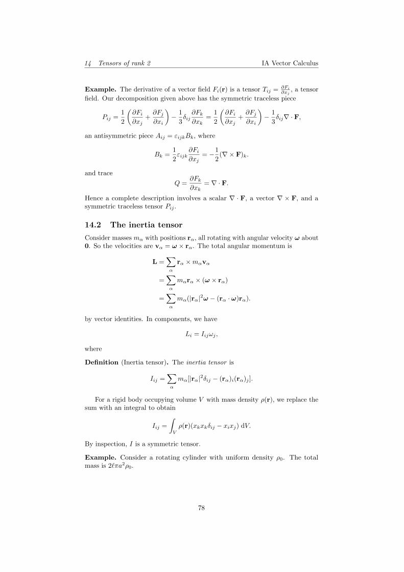
14 Tensors of rank 2 IA Vector Calculus
Example. The derivative of a vector field Fi(r) is a tensor Tij = ∂Fi
∂xj, a tensor
field. Our decomposition given above has the symmetric traceless piece
Pij =1
2
(∂Fi∂xj
+∂Fj∂xi
)− 1
3δij∂Fk∂xk
=1
2
(∂Fi∂xj
+∂Fj∂xi
)− 1
3δij∇ · F,
an antisymmetric piece Aij = εijkBk, where
Bk =1
2εijk
∂Fi∂xj
= −1
2(∇× F)k.
and trace
Q =∂Fk∂xk
= ∇ · F.
Hence a complete description involves a scalar ∇ · F, a vector ∇ × F, and asymmetric traceless tensor Pij .
14.2 The inertia tensor
Consider masses mα with positions rα, all rotating with angular velocity ω about0. So the velocities are vα = ω × rα. The total angular momentum is
L =∑α
rα ×mαvα
=∑α
mαrα × (ω × rα)
=∑α
mα(|rα|2ω − (rα · ω)rα).
by vector identities. In components, we have
Li = Iijωj ,
where
Definition (Inertia tensor). The inertia tensor is
Iij =∑α
mα[|rα|2δij − (rα)i(rα)j ].
For a rigid body occupying volume V with mass density ρ(r), we replace thesum with an integral to obtain
Iij =
∫V
ρ(r)(xkxkδij − xixj) dV.
By inspection, I is a symmetric tensor.
Example. Consider a rotating cylinder with uniform density ρ0. The totalmass is 2`πa2ρ0.
78

14 Tensors of rank 2 IA Vector Calculus
x1
x3
x2
2`
a
Use cylindrical polar coordinates:
x1 = r cos θ
x2 = r sin θ
x3 = x3
dV = r dr dθ dx3
We have
I33 =
∫V
ρ0(x21 + x2
2) dV
= ρ0
∫ a
0
∫ 2π
0
∫ `
−`r2(r dr dθ dx2)
= ρ0 · 2π · 2`[r4
4
]a0
= ε0π`a4.
Similarly, we have
I11 =
∫V
ρ0(x22 + x2
3) dV
= ρ0
∫ a
0
∫ 2π
0
∫ `
−`(r2 sin2 θ + x2
3)r dr dθ dx3
= ρ0
∫ a
0
∫ 2π
0
r
(r2 sin2 θ [x3]
`−` +
[x3
3
3
]`−`
)dθ dr
= ρ0
∫ a
0
∫ 2π
0
r
(r2 sin2 θ2`+
2
3`3)
dθ dr
= ρ0
(2πa · 2
3`3 + 2`
∫ a
0
r2 dr
∫ 2π
0
sin2 θ
)= ρ0πa
2`
(a2
2+
2
3`2)
By symmetry, the result for I22 is the same.
79

14 Tensors of rank 2 IA Vector Calculus
How about the off-diagonal elements?
I13 = −∫V
ρ0x1x3 dV
= −ρ0
∫ a
0
∫ `
−`
∫ 2π
0
r2 cos θx3 dr dx3 dθ
= 0
Since∫ 2π
0dθ cos θ = 0. Similarly, the other off-diagonal elements are all 0. So
the non-zero components are
I33 =1
2Ma2
I11 = I22 = M
(a2
4+`2
3
)In the particular case where ` = a
√3
2 , we have Iij = 12ma
2δij . So in this case,
L =1
2Ma2ω
for rotation about any axis.
14.3 Diagonalization of a symmetric second rank tensor
Recall that using matrix notation,
T = (Tij), T ′ = (T ′ij), R = (Rij),
and the tensor transformation rule T ′ij = RipRjqTpq becomes
T ′ = RTRT = RTR−1.
If T is symmetric, it can be diagonalized by such an orthogonal transformation.This means that there exists a basis of orthonormal eigenvectors e1, e2, e3 for Twith real eigenvalues λ1, λ2, λ3 respectively. The directions defined by e1, e2, e3
are the principal axes for T , and the tensor is diagonal in Cartesian coordinatesalong these axes.
This applies to any symmetric rank-2 tensor. For the special case of theinertia tensor, the eigenvalues are called the principal moments of inertia.
As exemplified in the previous example, we can often guess the correctprincipal axes for Iij based on the symmetries of the body. With the axes wechose, Iij was found to be diagonal by direct calculation.
80

15 Invariant and isotropic tensors IA Vector Calculus
15 Invariant and isotropic tensors
15.1 Definitions and classification results
Definition (Invariant and isotropic tensor). A tensor T is invariant under aparticular rotation R if
T ′ij···k = RipRjq · · ·RkrTpq···r = Tij···k,
i.e. every component is unchanged under the rotation.A tensor T which is invariant under every rotation is isotropic, i.e. the same
in every direction.
Example. The inertia tensor of a sphere is isotropic by symmetry.δij and εijk are also isotropic tensors. This ensures that the component
definitions of the scalar and vector products a·b = aibjδij and (a×b)i = εijkajbkare independent of the Cartesian coordinate system.
Isotropic tensors in R3 can be classified:
Theorem.
(i) There are no isotropic tensors of rank 1, except the zero tensor.
(ii) The most general rank 2 isotropic tensor is Tij = αδij for some scalar α.
(iii) The most general rank 3 isotropic tensor is Tijk = βεijk for some scalar β.
(iv) All isotropic tensors of higher rank are obtained by combining δij and εijkusing tensor products, contractions, and linear combinations.
We will provide a sketch of the proof:
Proof. We analyze conditions for invariance under specific rotations through πor π/2 about coordinate axes.
(i) Suppose Ti is rank-1 isotropic. Consider a rotation about x3 through π:
(Rij) =
−1 0 00 −1 00 0 1
.
We want T1 = RipTp = R11T1 = −T1. So T1 = 0. Similarly, T2 = 0. Byconsider a rotation about, say x1, we have T3 = 0.
(ii) Suppose Tij is rank-2 isotropic. Consider
(Rij) =
0 1 0−1 0 00 0 1
,
which is a rotation through π/2 about the x3 axis. Then
T13 = R1pR3qTpq = R12R33T23 = T23
81

15 Invariant and isotropic tensors IA Vector Calculus
andT23 = R2pR3qTpq = R21R33T13 = −T13
So T13 = T23 = 0. Similarly, we have T31 = T32 = 0.
We also haveT11 = R1pR1qTpq = R12R12T22 = T22.
So T11 = T22.
By picking a rotation about a different axis, we have T21 = T12 andT22 = T33.
Hence Tij = αδij .
(iii) Suppose that Tijk is rank-3 isotropic. Using the rotation by π about thex3 axis, we have
T133 = R1pR3qR3rTpqr = −T133.
So T133 = 0. We also have
T111 = R1pR1qR1rTpqr = −T111.
So T111 = 0. We have similar results for π rotations about other axes andother choices of indices.
Then we can show that Tijk = 0 unless all i, j, k are distinct.
Now consider
(Rij) =
0 1 0−1 0 00 0 1
,
a rotation about x3 through π/2. Then
T123 = R1pR2qR3rTpqr = R12R21R33T213 = −T213.
So T123 = −T213. Along with similar results for other indices and axes ofrotation, we find that Tijk is totally antisymmetric, and Tijk = βεijk forsome β.
Example. The most general isotropic tensor of rank 4 is
Tijk` = αδijδk` + βδikδj` + γδi`δjk
for some scalars α, β, γ. There are no other independent combinations. (wemight think we can write a rank-4 isotropic tensor in terms of εijk, like εijpεk`p,but this is just δikδj` − δi`δjk. It turns out that anything you write with εijkcan be written in terms of δij instead)
15.2 Application to invariant integrals
We have the following very useful theorem. It might seem a bit odd and arbitraryat first sight — if so, read the example below first (after reading the statementof the theorem), and things will make sense!
82

15 Invariant and isotropic tensors IA Vector Calculus
Theorem. Let
Tij···k =
∫V
f(x)xixj · · ·xk dV.
where f(x) is a scalar function and V is some volume.Given a rotation Rij , consider an active transformation: x = xiei is mapped
to x′ = x′iei with x′i = Rijxi, i.e. we map the components but not the basis, andV is mapped to V ′.
Suppose that under this active transformation,
(i) f(x) = f(x′),
(ii) V ′ = V (e.g. if V is all of space or a sphere).
Then Tij···k is invariant under the rotation.
Proof. First note that the Jacobian of the transformation R is 1, since it is
simply the determinant of R (x′i = Ripxp ⇒ ∂x′i∂xp
= Rip), which is by definition
1. So dV = dV ′.Then we have
RipRjq · · ·RkrTpq···r =
∫V
f(x)x′ix′j · · ·x′k dV
=
∫V
f(x′)x′ix′j · · ·x′k dV using (i)
=
∫V ′f(x′)x′ix
′j · · ·x′k dV ′ using (ii)
=
∫V
f(x)xixj · · ·xk dV since xi and x′i are dummy
= Tij···k.
The result is particularly useful if (i) and (ii) hold for any rotation R, inwhich case Tij···k is isotropic.
Example. Let
Tij =
∫V
xixj dV,
with V being a solid sphere of |r| < a. Our result applies with f = 1, which,being a constant, is clearly invariant under rotations. Also the solid sphere isinvariant under any rotation. So T must be isotropic. But the only rank 2isotropic tensor is αδij . Hence we must have
Tij = αδij ,
and all we have to do is to determine the scalar α.Taking the trace, we have
Tii = 3α =
∫V
xixi dV = 4π
∫ a
0
r2 · r2 dr =4
5πa5.
So
Tij =4
15πa5δij .
83

15 Invariant and isotropic tensors IA Vector Calculus
Normally if we are only interested in the i 6= j case, we just claim that Tij = 0by saying “by symmetry, it is 0”. But now we can do it (more) rigorously!
There is a closely related result for the inertia tensor of a solid sphere ofconstant density ρ0, or of mass M = 4
3πa3ρ0.
Recall that
Iij =
∫V
ρ0(xkxkδij − xixj) dV.
We see that Iij is isotropic (since we have just shown that∫xixj dV is isotropic,
and xkxkδij is also isotropic). Let Iij = βδij . Then
Iij =
∫V
ρ0(xkxkδij − xixj) dV
= ρ0
(δij
∫V
xkxk dV −∫V
xixj dV
)= ρ0 (δijTkk − Tij)
= ρ0
(4
5πa5δij −
4
15πa5δij
)=
8
15ρ0πa
5δij
=2
5Ma2δij .
84