part i. thermodynamics and statistical thermodynamicsaathavan/libraire/thermodynamicspri… · part...

Part I.

Thermodynamics and Statistical Thermodynamics

All of chemistry, including the chemistry of biological systems, can be viewed as being based on the interrelated physical factors of energetics, structure, and dynamics. In some ways, energetics can be viewed as most fundamental, since the energetic behavior of molecules determines their structure and reactivity. Thermodynamics is the branch of physical chemistry that systematizes the energetics of chemical systems at equilibrium, in terms of macroscopic concepts such as temperature, pressure, enthalpy, entropy, free energy, etc.

Biochemists and biophysicists are most often interested in the connection between structure and function of biological molecules. The bridge between the microscopic and macroscopic levels is provided by statistical mechanics or statistical thermodynamics. In this part we examine some applications of thermodynamics to biological systems, especially solutions of biologically interesting molecules, and describe how thermodynamic variables can be measured. We then discuss some of the major sources of noncovalent interactions in biomolecular systems, and how they can be estimated for interpretation of thermodynamic results. We conclude with a discussion of the statistical thermodynamics of polymer solutions.

Thermodynamic analysis of biopolymer systems

1 THERMODYNAMIC ANALYSIS OF BIOPOLYMER SYSTEMS

1-1 GOALS AND NATURE OF THERMODYNAMIC ANALYSIS

Molecular biophysics aims to understand the molecular basis of processes such as enzymatic conversions, ion transport, ligand binding, and conformational changes of proteins and nucleic acids, that make up the reactions occuring in biological systems. The aim of a thermodynamic analysis of a biomolecular system is to measure the changes in thermodynamic parameters such as free energy, enthalpy, entropy, and volume that occur during these processes, and to use these values to gain insight into the molecular interactions that regulate the process. Since biological systems are very complex, consisting of many complex, strongly interacting molecules, a full thermodynamic analysis would be very difficult. But useful progress can be made by some relatively simple considerations.

1-2 RELATION OF STANDARD FREE ENERGY CHANGE TO EQUILIBRIUM CONSTANT

A great deal of understanding can be obtained from systematic application of a few basic equations from thermodynamics. The first is the relation between equilibrium constant K and standard free energy change ∆G°:

(1-1)

which rearranges to the exponential form

(1-2)

This form emphasizes the importance of weak interactions, since small changes in ∆G° imply large changes in K. This can be seen explicitly by calculating various quantities for a unimolecular isomerization N , U where N might stand for the native form of a protein, and U for the unfolded form (or N for the base-paired helical form of a self-complementary single-stranded oligonucleotide, and U for the denatured or coil form)

As ∆G° (expressed in various units) ranges from somewhat positive to somewhat negative, we get

∆G° RT Kln–=

K e∆G°RT

-----------–=

α

K U[ ]N[ ]

--------- α1 α–------------= =

where α is the fraction denatured:

α U[ ]U[ ] N[ ]+

-------------------------K

1 K+-------------= =

-5 0 5

0.20

0.40

0.60

0.80

1.00

-∆G°/RT


∆G°/kJ ∆G°/kcal ∆G°/RT K7.43 1.78 3 0.050 0.0474.95 1.18 2 0.135 0.1192.48 0.59 1 0.368 0.2690.00 0.00 0 1.000 0.500

-2.48 -0.59 -1 2.718 0.731-4.95 -1.18 -2 7.389 0.881-7.43 -1.78 -3 20.086 0.953

Thus a change in ∆G° of 6 RT (only a few H-bonds or hydrophobic interactions) can change the fraction of the unfolded state from 5% to 95%.

It is worth noting the converse: Since ∆G° is related logarithmically to K, relatively crude measurement of K leads to quite accurate determination of ∆G°.

1-3 RELATION OF FREE ENERGY TO ENTHALPY AND ENTROPY

The second major equation is

(1-3)

This relates the Gibbs energy change to changes in standard enthalpy ∆H° and entropy ∆S°. In crude terms, ∆H° is related to the formation, breaking, or distortion of bonds; while ∆S° is related to the change in order or randomness in the system. A major effort in modern biophysics is understanding the molecular basis of the thermodynamic parameters ∆G°, ∆H°, and ∆S°.

1-4 DETERMINATION OF EQUILIBRIUM CONSTANT FROM LINEAR PROPERTIES

Measurable properties (e.g. spectral absorption, fluorescence, circular dichroism) are often linearly proportional to concentrations. A typical relation is the Beer-Lambert law for optical density A:

(1-4)

where is molar extinction coefficient, C is molar concentration, and l is path length. A similar equation holds for each species in the system, and the total optical density is the sum over all species. For the N , U transition, for example, we have (taking l = 1 cm)

(1-5)

where is the total protein concentration. This can be rearranged to solve for α:

(1-6)

It should be emphasized that this treatment assumes that the only states contributing are N and U; that is, that this is a two-state transition. This is a very common assumption in biochemistry, but needs to be examined carefully in each particular case, since it may not always be true.

∆G° ∆H° T∆S°–=

A Cl=

A AN AU+ εN N[ ] U U[ ]+ N 1 –( ) U+[ ]CT= = =

CT

αA εNCT–

εUCT εNCT–---------------------------------

A AN–

AU AN–---------------------= =


1-5 DETERMINING ∆H° AND ∆S° FROM THE VAN'T HOFF EQUATION

If we can measure K as a function of T, we can determine the other thermodynamic parameters. The starting point is the van't Hoff equation, which may be derived as follows. We divide Eq. (1-3) by T

(1-7)

and then differentiate

. (1-8)

We recall that

(1-9)

and is the heat capacity at constant pressure P so that

(1-10)

Substituting these relations in eq. (1-8) we get

(1-11)

Now using eq. (1-1), we finally obtain the van’t Hoff equation which can be written in either of the two equivalent forms

(1-12)

where the second form comes from noting that . The first form of the van’t

Hoff equation makes it easy to see (and remember) that for an endothermic reaction (∆H° > 0), lnK increases with T; while the second form suggests a linear plot of lnK vs 1/T to obtain ∆H°:

∆GT

--------∆HT

-------- ∆S–=

Tdd ∆G

T--------

1T---

Tdd ∆H

∆HT2--------–

Tdd ∆S–=

dH δQ and dSδQT

------- where δQ CPdT= = =

CP

d∆H ∆CPdT and d∆S∆CP

T-----------dT= =

Tdd ∆G

T--------

∆CP

T-----------

∆HT2--------–

∆CP

T-----------–

∆HT2--------–= =

Kln∂T∂

------------∆H°RT 2----------- or

Kln∂1 T⁄( )∂

------------------∆H°

R-----------–==

T∂∂ 1

T2------

1 T⁄( )∂∂

–=

lnK

1/T

slope = -∆H°/R


Once the standard free energy and enthalpy changes are known, the entropy change is obtained from

. (1-13)

1-6 DETERMINING THERMODYNAMIC PARAMETERS FROM REACTION PROGRESS AND MOLECULARITY

In many cases, it is the fractional reaction rather than K that is measured directly. Further, determining K from requires a knowledge of n, the number of molecules in the reaction. That is, for proteins one can consider unfolding (n=1), dimerization (n=2), tetramerization (n=4), etc. For nucleic acids, one can consider melting of an intramolecular hairpin (n=1), melting of a duplex (n=2), melting of a triplex or tetraplex, etc. A general analysis for determining thermodynamic parameters from n and the T-dependence of has been developed by Marky & Breslauer (1,2).

A distinction must be made between identical and non-identical reaction partners. Consider first identical partners, such as self-complementary oligonucleotides or protein oligomers composed of identical subunits, undergoing the reaction n A , An. Let be the fraction of A chains in state An, where the total molar concentration of chains is CT. The equilibrium expression

is

(1-14)

If we define the "melting" temperature T m as that at which α = 1/2, then we see that

(1-15)

which allows determination of K from the total monomer concentration at the midpoint of the transition. The van't Hoff equation can be obtained in terms of by taking logarithms of both sides

of eq (1-14) and differentiating, noting that nCTn-1 is a constant:

(1-16)

∆HvH is thus related to the slope at the midpoint, where = 1/2, by

(1-17)

The numerical coefficient (2 + 2n) is 4 for a unimolecular process, 6 for dimerization, etc.If the reaction is between n non-identical chains, each at molar concentration CT/n,

∆S° ∆H° ∆G°–( )T

---------------------------------=

KAn[ ]A[ ]n

-----------α CT n⁄( )1 α–( )CT[ ]n

-------------------------------- αnCT

n 1– 1 α–( )n-------------------------------------= = =

K Tm( ) 1n CT 2⁄( )n 1–-------------------------------=

∆HvH R∂ Kln

∂ 1 T⁄( )------------------– R

∂∂ 1 T⁄( )------------------ αln n 1 α–( )ln–[ ]– R

1α--- n

11 α–------------+

∂α∂ 1 T⁄( )------------------–= = =

∆HvH R 2 2n+( ) ∂α∂ 1 T⁄( )------------------

T Tm=–=


(1-18)

the equilibrium expression is

(1-19)

This differs from eq (1-14) for identical chains, but the dependence on is the same, so eq (1-17) holds for both cases.

1-7 DIFFERENTIAL SCANNING CALORIMETRY (DSC)

Biological samples are usually small and dilute, so conventional calorimetric measurements have until recently required too much material and have lacked sensitivity. However, recent technical advances have led to the development of microcalorimeters, which can detect the very small amounts of heat generated or consumed by the ligand binding and conformational change reactions undergone by proteins, nucleic acids, and membranes. Binding reactions are generally studied by isothermal titration calorimeters, which will be described later. Here we consider differential scanning calorimeters, in which processes such as protein unfolding and helix-coil transitions can be studied as a function of temperature (3). A schematic diagram of a differential scanning calorimeter is shown below:

Heat is supplied at the same rate to two matched cells. The solution cell will generally absorb more heat than the buffer cell, causing a slight difference in temperature ∆T between the two cells. A feedback loop monitoring T will supply a small amount of heat ∆Q to the solution cell, so as to equalize the temperatures. The heat capacity ∆Cp = ∆Q/∆T.

Determination of ∆H and ∆S from DSCA schematic illustration of how DSC traces are integrated to obtain enthalpy and entropy:

Note how the same data (CP as a function ot T) can be used to obtain both ∆H and ∆S, and thereby ∆G as well.

A1 A2 A3 …An+ + + , A1A2A3…An

KA1A2A3…An[ ]

A1[ ] A2[ ] A3[ ]… An[ ]----------------------------------------------------

α CT n⁄( )1 α–( ) CT n⁄( )[ ]n

-------------------------------------------- αCT n⁄( )n 1– 1 α–( )n

------------------------------------------------= = =

T1 T2

baselinesubtracted

Cp = ∆Q∆T

T

area = ∆Hcal = ∫Cp dT

T2

T1

∆S = ∫ ( Cp/T) dTCp

T

T

T2

T1


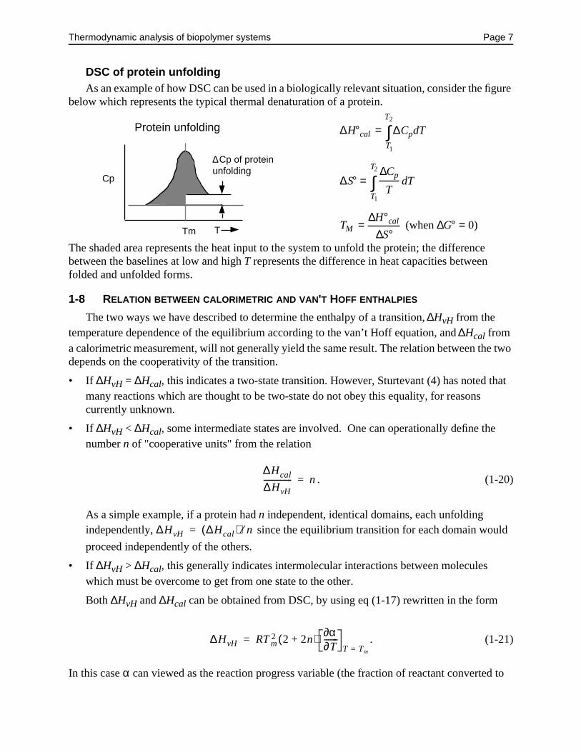
DSC of protein unfoldingAs an example of how DSC can be used in a biologically relevant situation, consider the figure

below which represents the typical thermal denaturation of a protein.

The shaded area represents the heat input to the system to unfold the protein; the difference between the baselines at low and high T represents the difference in heat capacities between folded and unfolded forms.

1-8 RELATION BETWEEN CALORIMETRIC AND VAN'T HOFF ENTHALPIES

The two ways we have described to determine the enthalpy of a transition, ∆HvH from the temperature dependence of the equilibrium according to the van’t Hoff equation, and ∆Hcal from a calorimetric measurement, will not generally yield the same result. The relation between the two depends on the cooperativity of the transition.

• If ∆HvH = ∆Hcal, this indicates a two-state transition. However, Sturtevant (4) has noted that many reactions which are thought to be two-state do not obey this equality, for reasons currently unknown.

• If ∆HvH < ∆Hcal, some intermediate states are involved. One can operationally define the number n of "cooperative units" from the relation

. (1-20)

As a simple example, if a protein had n independent, identical domains, each unfolding independently, since the equilibrium transition for each domain would

proceed independently of the others.

• If ∆HvH > ∆Hcal, this generally indicates intermolecular interactions between molecules which must be overcome to get from one state to the other.

Both ∆HvH and ∆Hcal can be obtained from DSC, by using eq (1-17) rewritten in the form

. (1-21)

In this case α can viewed as the reaction progress variable (the fraction of reactant converted to

Cp

TTm

∆Cp of protein unfolding

Protein unfolding ∆H°cal = ∆CpdTT1

T2

∫

∆S° =∆Cp

TdT

T1

T2

∫

TM =∆H°cal

∆S° (when ∆G° = 0)

∆Hcal

∆HvH-------------- n=

∆HvH ∆Hcal( ) n⁄=

∆HvH RT m2 2 2n+( ) ∂α

∂T-------

T Tm==


product), which can be evaluated from the heat capacity curve

(1-22)

and

(1-23)

where CP,ex(Tm) is the excess heat capacity at the half-way point of the transition (approximately the maximum in the CP vs T curve).

1-9 REFERENCES

1. Marky, L. A. & K. J. Breslauer (1987) Calculating thermodynamic data for transitions of any molecularity from equilibrium melting curves. Biopolymers 26: 1601-1620

2. Breslauer, K.J. (1995) Extracting thermodynamic data from equilibrium melting curves for oligonucleotide order-disorder transitions. Meth. Enzymol. 259: 221-242.

3. Sturtevant, J. M. (1987). Biochemical applications of differential scanning calorimetry. Annu. Rev. Phys. Chem. 38: 463-488.

4. Liu, Y. F. & J. M. Sturtevant. (1995). Significant discrepancies between van't Hoff and calorimetric enthalpies .2. Protein Sci. 4: 2559-2561.

α T( ) 1∆Hcal-------------- CP Td

T1

T

∫= so that ∂α∂T-------

T Tm=

CP ex, Tm( )∆Hcal

-------------------------=

∆HvH 2n 2+( )RT m2

CP ex, Tm( )∆Hcal

-------------------------=

Thermodynamics of solutions

2 THERMODYNAMICS OF SOLUTIONS

Much of biophysical chemistry is concerned with the thermodynamic changes that occur when a residue is moved from one environment to another, e.g., a nonpolar amino acid from the interior of a native protein to the aqueous solvent in the unfolded protein. Volumes and densities change when components of biomolecular solutions are mixed, and changes in concentrations and pressure cause changes of osmotic pressure and water activity. Proper treatment of these types of changes requires consideration of the thermodynamics of solutions, the topic of this chapter.

2-1 CONCENTRATION SCALES

There are many ways of describing the concentration of a solution, each useful in different situations. We will use ni, Ni, gi, and Mi to denote the number of moles, molecules, grams, and molecular weight of component i in the solution.

Mole fractionThe most useful concentration variable for theoretical understanding of solutions of like-sized

molecules is the mole fraction X:

(2-1)

MolalityThe molality mB is the moles of component B per kg (1000 g) of some other component A

chosen as solvent. It is the most direct for accurate preparation of solutions by weight, since it is not affected by solution volume change on mixing. The relation between solute mole fraction and molality in binary solution is

(2-2)

MolarityThe molarity CB is the number of moles of B per liter of solution. This is experimentally

convenient if solutions are prepared by volume; and statistical thermodynamic theories are also usually developed for a defined volume. If the solution density (g/mL or kg/L) = , the relation between mole fraction and molarity in a binary solution is

(2-3)

Weight concentrationThe weight concentration cB is the grams of B per liter of solution (or mg/mL in common

biochemical usage). It is useful when you don't know the molecular weight, and you make up

XA

nA

nA nB nC …+ + +-------------------------------------------

nA

nA nB+------------------ in binary solution.= =

XB

mB

1000MA

------------ mB+--------------------------

mBMA

1000---------------- in dilute solutions.→=

XB

CB

1000ρ CBMB–

MA------------------------------------- CB+

---------------------------------------------------CBMA

1000ρA------------------ for dilute solutions→=


solutions by volume rather than by weight. Of course, cB = CBMB. Some variants are g/mL =

(for calculations in cgs units), g/100 g solution = weight percent, and g/dL = cB/10 ≈

weight percent in water

Volume fractionThe volume fraction φ is often used for polymer solutions, where the solute (polymer,

component 2) is much larger than the solvent (component 1). If each segment of the polymer is the same size as a solvent model (commonly assumed in lattice models, though not generally true), and there are σ segments per polymer,

. (2-4)

2-2 EXTENSIVE AND INTENSIVE QUANTITIES

Thermodynamic description of a system involves extensive quantities (state functions), which are proportional to the size of the system; and intensive quantities, which are not. The usual extensive quantities are volume V, internal energy E, enthalpy H, Gibbs (free) energy G, entropy S, and Helmholz energy A, and the number of moles of each component. In membrane or bilayer systems the surface area is also an extensive quantity.

The usual intensive quantities are pressure P, temperature T, partial molar quantities, and applied fields (electric, magnetic, centrifugal, etc.).

2-3 PARTIAL MOLAR QUANTITIES

Because of interactions between components, the value of an extensive quantity in a solution is generally not equal to the sum of the values for the pure components. To deal with this situation, we use partial molar quantities.

For example, the partial molar volume of component A is the change in volume of a solution upon adding one mole of A to a volume of solution large enough that the concentration is not changed appreciably, at constant T and P.

. (2-5)

Adding dnA moles of A and dnB moles of B to a solution produces a volume change

. (2-6)

This expression can be integrated, increasing the volume while maintaining the relative

composition constant, so and don't change:

(2-7)

cB 1000⁄

φ1

n1

n1 σn2+---------------------= and φ2

σn2

n1 σn2+---------------------=

V A

V A∂V∂nA---------

T P nB, ,

=

dV∂V∂nA---------

T P nB, ,

dn A∂V∂nB---------

T P nA, ,

dn B+ V Adn A VBdn B+= =

V A VB

V nAV A nBVB+=


(rather than the sum for the pure components).

Gibbs-Duhem equationThe total differential of eq (2-7) is

. (2-8)

Comparison with eq (2-6) yields one form of the Gibbs-Duhem equation:

. (2-9)

Generalizing from a binary solution to an n-component system, this states that one of the partial molar quantities can be obtained from the n concentrations and (n-1) other partial molar quantities.

Partial molar quantities corresponding to other extensive variablesThe same relations hold for the other extensive state variables, e.g.:

. (2-10)

The last of these equations defines the chemical potential µA, which we will use extensively later.

Maxwell equationsFor one-component thermodynamics one has the relations

(2-11)

Differentiating again with respect to the number of moles of component i, one gets the basic thermodynamic relations for solutions

, (2-12)

and so forth. These cross-derivative relations are examples of Maxwell relations.

2-4 EXPERIMENTAL DETERMINATION OF PARTIAL MOLAR QUANTITIES

We will take partial molar volume as an example; other partial molar quantities are calculated

exactly the same way. If B is water and A is solute, is the slope when the volume of solution is plotted against the molality of A (at constant 1 kg of B). The direct numerical differentiation of

V with respect to mA is not very accurate. A better way is to calculate as some average V plus a correction term. One standard way is the "method of intercepts".

nAV A° nBVB°+

dV V Adn A nAdV A VBdn B nBdV B+ + +=

nAdV A nBdV B+ 0 or dV AnB

nA------dV B–= =

SA∂S

∂nA---------

T P nB, ,

= , HA∂H∂nA---------

T P nB, ,

, GA∂G∂nA---------

T P nB, ,

== µA=

∂G∂P-------

T

V ; ∂GdT-------

P

S; ∂H∂T-------

P

– CP= = = ; etc

∂Gi

∂P---------

T

∂µ i

∂P--------

T

V i= = ; ∂µ i

∂T--------

P

Si–= ; ∂Hi

∂T---------

CPi=

V A

V A


Define the molar volume of solution as the volume per total number of moles of all components:

. (2-13)

Thus

. (2-14)

By the chain rule,

(2-15)

Combination of eqs (2-14) and (2-15) yields

(2-16)

Thus if a plot is constructed of vs XB, and a line is drawn tangent to the curve at any point, the

intercept at XB = 0 is , and the intercept at XB = 1 is . If is known as a function of

concentration, can also be calculated by numerical integration of the Gibbs-Duhem equation:

. (2-17)

Note that the partial molar volume (and other partial molar quantities) are not constants, but

will be functions of concentration. In the dilute solutions most often studied in biochemistry,

of the solvent is often well approximated by the value for pure solvent, ; while of the

solute has its limiting, infinite dilution value which may be quite different from that for pure B.

2-5 CHEMICAL POTENTIAL

The chemical potential

(2-18)

V

V VnA nB+------------------= V→ V nA nB+( )=

V A∂V∂nA---------

nB

V∂V∂nA---------

nB

nA nB+( )+= =

∂V∂nA---------

nB

∂V∂XB----------

∂XB

∂nA----------

nB

∂V∂XB----------

nB

nA nB+( )2--------------------------–= =

V V A XB∂V

∂XB----------

+=

V

V A VB V A

VB

VBd∫nA

nB------ V Ad∫–

XA

XB------- V Ad∫–= =

V A

V A° VB

µi Gi∂G∂ni-------

T P n j i≠, ,

= =


is the key quantity in solution thermodynamics. One learns in basic physical chemistry that if a

component is in equilibrium between two phases α and β at the same T and P, .

Derivatives of µ i with respect to T and P give

(2-19)

2-6 THERMODYNAMICS OF MIXING

When pure components are mixed to form a solution, the change in a thermodynamic quantity such as the enthalpy is called the enthalpy of mixing, ∆Hmix. It is the difference between the enthalpy of the solution and the pure components:

. (2-20)

Similar equations hold for the volume of mixing ∆Vmix, the entropy of mixing ∆Smix, and so on.

Note that because , the Gibbs energy of mixing can be written

. (2-21)

2-7 IDEAL SOLUTIONS

An ideal solution is one in which all molecules have the same intermolecular forces and volumes, so that ∆Hmix = 0 and ∆Vmix = 0. Then the molecules in the solution can mix totally randomly, and all the thermodynamic properties of the solution, relative to the pure components, can be calculated from the entropy of mixing.

Entropy of mixing of an ideal solutionConsider the bringing together of N1 molecules of 1 and N2 molecules moles of 2 from the

pure liquids to form a mixture with mole fraction X1 = N1/(N1 + N2) and .

Use the Boltzmann equation

(2-22)

and a lattice model (not required, but simple) to calculate S for the pure components and the mixture. Ω is the number of distinguishable configurations of the system, and kB is the Boltzmann constant. Since all the molecules in the pure components are identical, there is only one distinguishable way to arrange them, so Ω = 0 and .

For the mixture, let N0 = N1 + N2 be the total number of lattice sites. Imagine placing the 1 molecules first: There are N0 sites on which to place the first, (N0 - 1) for the second, (N0 - 2) for the third, and (N0 - N1 + 1) for the N1th.The total number of ways to place the type 1 molecules is the product of all of these: N0(N0 - 1)(N0 - 2) … (N0 - N1 + 1). Since all molecules of type 1 are identical, the number of distinguishable ways to place them on the lattice is

µiα µi

β=

∂µ i

∂P--------

T n j i≠,

V i=∂ µi T⁄( )∂ 1 T⁄( )--------------------

P n j i≠,, Hi=

∂µ i

∂T--------

P n j i≠,

, Si–=

∆Hmix Hsolution niHi°∑– niHi∑ niHi°∑– ni Hi Hi°–( )∑= = =

Gi µi=

∆Gmix ni µi µi°–( )∑=

X2 N2 N1 N2+( )⁄=

S kB Ωln=

S1° S2° 0= =


(2-23)

(The molecules of type 2 are then added to all empty sites, but there is only one distinguishable way to do this.) To evaluate Ssolution, we take the logarithm of Ω, using Stirling's approximation

(2-24)

which is very accurate for large N. This yields (remember N0 = N1 + N2)

(2-25)

or

(2-26)

where NA is the Avogadro number and R is the gas constant. Then

(2-27)

for an ideal solution.If the solution has c components, this can readily be generalized to

(2-28)

Differentiation of Ssolution with respect to ni yields

(2-29)

If there are different interactions between different types of molecular pairs, or if they occupy different volumes, then mixing will not be totally random (there will be clustering) and the entropy of mixing will be different than the ideal value. This is the case in most biologically relevant systems.

Chemical potential in ideal solutions

Since , one can write for ideal solutions

(2-30)

ΩN0 N0 1–( ) N0 2–( )… N0 N1– 1+( )

N1!-----------------------------------------------------------------------------------------

N0!

N1!N2!------------------= =

N!( ) N Nln N–≈ln

Ωln N0 N0ln N0–( ) N1 N1ln N1–( ) N2 N2ln N2–( )––

N1

N1

N1 N2+-------------------- N2

N2

N1 N2+--------------------ln–ln–

=

=

Ssolution NAkB– n1 X1ln n2 X2ln+( ) R n1 X1ln n2 X2ln+( )–= =

∆Smix Ssolution S1°– S2°– R n1 X1ln n2 X2ln+( )–= =

∆Smix Ssolution R ni Xilni 1=

c

∑–= =

Si R Xiln–=

µi Hi TS i–=

µi µi° T P,( ) RT Xiln+=


where the standard chemical potential refers to the state in which Xi =1. Expressions

other than eq (2-30) are frequently written, since in dilute solution Xi, Ci, ci, and mi are all proportional to each other if i is solute. Thus for example

(2-31)

where the standard chemical potential in the reference state of 1 mol/L differs from the standard chemical potential in the reference state of Xi = 1 by a constant. Since we are generally concerned

with differences in chemical potential during reactions or transfer processes, usually

cancels out.

2-8 ACTIVITIES AND ACTIVITY COEFFICIENTS IN REAL SOLUTIONS

In real solutions the molecules are generally different in intermolecular forces and volumes, leading to non-zero ∆Hmix and ∆Vmix. This nonideal behavior can be subsumed in an activity coefficient which is a function of concentrations as well as T and P, and the concentration is generalized to an activity. The activity coefficient → 1, and the activity approaches the concentration, as the solution approaches the standard state.

(2-32)

where

(2-33)

depending on concentration scale. If component i is solvent, the usual standard state is pure solvent, so γi → 1 as Xi → 1. If component i is solute, the properties of the standard state are usually those at infinite dilution. If one is using mole fraction as concentration variable, the standard state is then XB = 1, pure solute but with the properties of solute completely surrounded by solvent molecules.

2-9 CHEMICAL POTENTIAL AND VIRIAL EXPANSION

Another way to describe solution nonideality is through a concentration expansion. Even for an ideal solution, it may be necessary to carry higher terms in the expansion:

(2-34)

In dilute solutions one has n2 « n1, so one can express the solute concetration in molar or molal units rather than mole fractions as

(2-35)

µi° T P,( )

µi µi° T P,( ) RT Ciln+=

µi° T P,( )

µi µi° T P,( ) RT ailn+=

ai γ iXi= or ai yiCi=

µ1 µ1°– RT X1ln RT 1 X2–( )ln RT X212---X2

2 …+ + –= = =

X2

n2

n1-----≈ C2V1°

c2V1°M2

--------------= =


where is the molar volume (liters/mole) of pure solvent. Then one has the virial expansion in

powers of c2

(2-36)

The generalization of this to nonideal solutions is

(2-37)

where B is the second virial coefficient, C is the third, etc. B characterizes nonideal interactions between pairs of molecules, C characterizes 3-body effects, etc.

2-10 EFFECTS OF HYDROSTATIC PRESSURE

Biological reactions that involve changes in the exposure of charged or nonpolar groups often proceed with a change in volume, ∆V. If high pressure P (hundreds or thousands of atmospheres are readily attained) is imposed on a solution, sizeable changes in the position of equilibrium can occur (1). The equation governing this is simply that for P-V work:

(2-38)

2-11 OSMOTIC PRESSURE AND ITS RELATION TO CHEMICAL POTENTIAL

Osmotic pressure is a common way to measure the chemical potential of polymer solutions. If polymer in solvent is separated by pure solvent by a semipermeable membrane, the polymer lowers the chemical potential of the solvent. A pressure applied to the polymer compartment raises µ1 until equilibrium is reestablished and the solvent chemical potential is the same on both sides of the membrane. The excess pressure above atmospheric is called the osmotic pressure ∏.

From analogy with the increase in Gibbs energy with

pressure, dG = VdP, a term must be added to µ1 to account for the excess pressure. This increase in µ1 just compensates the decrease in µ1 due to the presence of the solute, given by the right hand side of eq (2-37). Thus we find

(2-39)

The value of Π/c2 extrapolated to c2 = 0 is RT/M2, which shows how osmotic pressure can be used to determine molecular weight.

V1°

µ1 µ1°– RTV 1°c2

M2------- 1

V1°2M2-----------c2 …+ +

–=

µ1 µ1°– RTV 1°c2

M2------- 1 Bc2 Cc2

2 …+ + +( )–=

∆G P∆V or K P( ) K 1 atm( )e P∆V RT⁄–= =

Polymer + solvent

puresolvent

∏

V1Π

ΠRTc2

M2------------- 1 Bc2 Cc2

2 …+ + +( )=


Osmotic pressure is sometimes expressed in osmolality. Using the infinite dilution limiting forms Π = RTc2/M2 = RTC2, and expressing R as 0.082 L-atm/mol-K and C2 in mol/kg H20, we find that 1 osmol = 24 atm at 20 C.

2-12 OSMOTIC STRESS AND WATER ACTIVITY

Osmotic pressure as described above is an effect of dissolved solute on the activity of water. The equivalent of osmotic pressure can be exerted without a semipermeable membrane, if a solute added to an aqueous solution has no significant effect other than lowering the activity of water. Such solutes are called osmolytes. According to a useful review by Parsegian et al. (2), they include “several different polyethylene glycols, from Mr 100 to 20,000, methylated PEG, polyvinylpyrrolidone, several dextrans, stachyose, sucrose, glucose, trehalose, sorbitol, glycerol, betaine, glycine, and even NaCl.” Osmotic pressures, expressed as osmolalities, are conveniently measured by vapor pressure osmometry (Wescor) as well as by freezing point depression and other techniques. A database of osmotic pressures for many osmolytes is maintained on two WWW sites: http://aqueous.labs.brocku.ca/osfile.html and http://abulafia.mgsl.dcrt.nih.gov/start.html.

The important aspect of these molecules is that they strongly lower the activity of water (generally by being strongly hydrated, thus effectively “removing” water from solution) while not interacting significantly with the biopolymers or ionic constituents of interest. The relation between water activity and osmotic pressure, from previous equations in this section, is simply

. (2-40)

There is a great deal of current research on the effect of osmolytes on a wide range of biochemical processes, arising from the realization that water is an important participant in most such reactions, along with protons, ions, and small ligands (2,3). We shall discuss some of the effects of water activity in later sections.

It no longer suffices to assert that since water is about 55 M, it is present in unchanging excess. It can been cogently argued that the osmotic pressure of solutions should be routinely measured along with pH, temperature, pressure, and ionic composition.

2-13 REFERENCES

1. Royer, C. (1995). Application of pressure to biochemical equilibria: The other thermodynamic variable. Meth. Enzymol. 259: 357-377.

2. Parsegian, V. A., R. P. Rand & D. C. Rau. (1995). Macromolecules and water: Probing with osmotic stress. Meth. Enzymol. 259: 43-94.

3. Robinson, C. R. & S. G. Sligar. (1995). Hydrostatic and osmotic pressure as tools to study macromolecular recognition. Meth. Enzymol. 259: 395-427.

µw µw°– RT awln VwΠ–= =

Estimating molecular contributions to thermodynamic properties

3 ESTIMATING MOLECULAR CONTRIBUTIONS TO THERMODYNAMIC PROPERTIES

Although thermodynamic information is useful in its own right for analysis of biochemical systems, much of the activity in this area is devoted to developing molecular interpretations of thermodynamic data. This will enable, it is hoped, a direct link between molecular structure and functional properties. Because biopolymers and aqueous solutions are so complex, the goal of adequate molecular understanding is far from realization. However, the attempts thus far have given useful insight.

3-1 INTERNAL ENERGY TERMS FOR MOLECULAR DYNAMICS CALCULATIONS

There are at least two main approaches to understanding the molecular basis of energetics of biomolecular systems. The most direct and fundamental is to express interactions between all pairs of atoms in terms familiar from small molecules: bond stretching, bending, and twisting; Lennard-Jones interactions, coulombic interactions, and hydrogen bonding. Direct quantum-mechanical calculation of these interactions is currently out of the question, so parameters (force fields) are adjusted for good agreement with experiments on small molecules containing similar atomic groupings and with an increasing body of quantum mechanical results. A typical force field used in molecular dynamics computer programs such as AMBER and CHARMM has the following internal energy (potential energy) terms:

: (3-1)

The coefficients in these equations are adjusted empirically. In current work, agreement with experiment is (in selected cases) within a few kcal, which is excellent considering that the beginning and end states of a transition each have energies of thousands of kcal. However, since 1.4 kcal of free energy can displace the equilibrium by a factor of ten, even this excellent agreement is not generally adequate for reliable prediction.

3-2 ADDITIVE APPROACH TO NONCOVALENT INTERACTIONS

Molecular dynamics calculations for proteins and nucleic acids are extremely demanding, requiring hundreds of hours on the fastest supercomputers. Therefore, many approximate estimates of enthalpy and free changes in biochemical reactions are made by ignoring bonded interactions (stretching, bending, torsion) and using typical values for the noncovalent interactions which are thought to dominate energy and entropy changes in biochemical reactions. Approximate values are given in the table on the next page, along with dependence of some of the

Vtotal =12 Kr(r – req)2 + 1

2 K ( – eq)2Σangles

+ 12 Vn 1 + cos (n – )Σ

torsionsΣ

bonds

+Aij

Rij12 –

Bij

Rij6 +

qiq j

RijΣj= 1

i – 1

Σi = 2

N+

Cij

Rij12 –

Dij

Rij10Σ

j= i

i – 1

Σi = 2

N

Van der Waals(Lennard-Jones)

Coulombic H-bonding


interactions on interatomic distance r, charge q, dipole moment µ, angle θ between dipoles, polarizability α, and dielectric constant ε.

Several things are worth noting about this table. First, the approximate energy values vary widely, certainly enough to seriously affect the estimation of an equilibrium constant. Second, the last three interactions do not have equations, since they are not readily reducible to simple forms. (Hydrogen bonding may obey an interaction equation as in eq (3-1), but this is in a vacuum, while the value given in the table is pertinent to aqueous solution where water competes for H-bonds.) Third, the hydrophobic and hydration forces are largely entropic rather than enthalpic; these “collective interactions” will be discussed in more detail below.

3-3 ENTROPY CHANGES IN BIOCHEMICAL REACTIONS

The position of chemical equilibrium is determined by the free energy change which contains both enthalpic and entropic contributions: . Entropy is usually just as important as enthalpy, but is often harder to understand and calculate adequately.

Translational entropyIn a bimolecular reaction, such as ligand binding to a macromolecule or dimerization of a

protein, the individual translational entropy of the two partners is lost and converted to the translational entropy of the complex. Even for such an apparently simple and fundamental process, there is active disagreement (3-5) about how to calculate the translational entropy change ∆St in aqueous solution.

According to one point of view (3,4) the solvent, being composed of indistinguishable molecules, plays no essential role in the translational motion of solute molecules. Thus one can use the Sackur-Tetrode equation for the translational entropy of an ideal monatomic gas:

(3-2)

for N molecules of mass m in volume V, where e is the base of natural logarithms and h is Planck’s constant. (This equation is in cgs units. To convert to molar units with standard state 1 mol/L, use N = NA, molecular mass m = M/NA, V = 1000 mL, and note that NAkB = R, the gas constant.)

In forming a bimolecular complex between reactants of mass m1 and m2,

TYPICAL MAGNITUDES OF NONCOVALENT INTERACTIONS

Type Equation Approx kcal/molIon-ion q1q2/εr 14 (ε = 8, r = 3 Å)Ion-dipole q1µ2f(θ)/εr2 -2 to +2 (µ = 2 debye)Dipole-dipole µ1µ2f'(θ)/εr3 -0.5 to 0.5Ion-induced dipole q12α2/2ε2r4 0.06 (α = 2x10-24 cm3)Dispersion, and stacking of aromatic ring systems

3hν0α3/4r6 0 to 10

H-bonding -1.3 ± 0.6 per H-bond1

Hydrophobic -1.3 ± 0.5 per CH22

Hydration force -0.1 to 0.1 per residue

∆G° ∆H° T∆S°–=

St m( ) Nk B

2πmk BT

h2---------------------

3 2/ Ve5 2/

N--------------ln=


. (3-3)

According to the other point of view (5), the proper entropy change is that calculated using the ideal solution entropy of mixing expression, eq (2-28), since the entropy change in solution is considered to be due to the various distinguishable arrangements of solvent and solute molecules. For the general reaction

(3-4)

with X = equilibrium mole fraction of product P, manipulation of eq (2-28) gives

(3-5)

If the standard state is 1 molar in water, then X = 1/55.5 and RlnX = - 8 cal mol-1 K-1. These two treatments lead to quite different numerical results, so which one is chosen has considerable practical importance. Although there are good scientists on both sides of this arguments, I will place my bets on the Sackur-Tetrode treatment.

Rotational entropyIf a dimer is formed from two monomers, the rotational entropy of the monomers is lost, and

that of the dimer is gained. This is sometimes estimated from the statistical mechanical expression for the rotational entropy of nonlinear molecules

(3-6)

where I is an average moment of inertia ≈ mr2 where r is a typical dimension of the molecule. The rotational entropy change is only infrequently taken into account in calculating the thermodynamics of complex formation.

Conformational entropy of backbone and side chainsWhen a protein folded in its native conformation, or a helical polypeptide, is converted to an

unfolded state, the peptide backbone gains conformational entropy due to the increased number of rotational isomeric states accessible to each backbone unit. The entropy increase can be estimated from the Boltzmann equation if it is assumed that each of n backbone bonds has ω rotational isomeric states in the unfolded conformation, but only one rotational state in the folded conformation. Then

(3-7)

since Ωfolded = 1. For example, each peptide group in the polypeptide backbone has two rotatable bonds (the φ and ψ angles), each of which has approximately 3 rotational isomeric states. Thus if np is the number of amino acids in the polypeptide, n = 2np and ω ≈ 3.

∆St St m1 m2+( ) St m1( )– St m2( )–=

iA jB … kC+ + + P,

∆St R i j … k 1–+ + +( ) Xln R i iln j jln … k kln+ + +( )+=

Sr32---Nk B

8π2Ik BT

h2----------------------

ln=

∆Sconf Sunfolded S folded– kB Ωunfoldedln kB ωnln nk B ωln= = = =


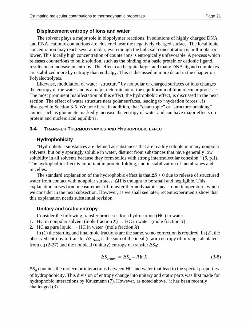
Displacement entropy of ions and waterThe solvent plays a major role in biopolymer reactions. In solutions of highly charged DNA

and RNA, cationic counterions are clustered near the negatively charged surface. The local ionic concentration may reach several molar, even though the bulk salt concentration is millimolar or lower. This locally high concentration of counterions is entropically unfavorable. A process which releases counterions to bulk solution, such as the binding of a basic protein or cationic ligand, results in an increase in entropy. The effect can be quite large, and many DNA-ligand complexes are stabilized more by entropy than enthalpy. This is discussed in more detail in the chapter on Polyelectrolytes.

Likewise, modulation of water “structure” by nonpolar or charged surfaces or ions changes the entropy of the water and is a major determinant of the equilibrium of biomolecular processes. The most prominent manifestation of this effect, the hydrophobic effect, is discussed in the next section. The effect of water structure near polar surfaces, leading to “hydration forces”, is discussed in Section 3-5. We note here, in addition, that “chaotropic” or “structure-breaking” anions such as glutamate markedly increase the entropy of water and can have major effects on protein and nucleic acid equilibria.

3-4 TRANSFER THERMODYNAMICS AND HYDROPHOBIC EFFECT

Hydrophobicity"Hydrophobic substances are defined as substances that are readily soluble in many nonpolar

solvents, but only sparingly soluble in water, distinct from substances that have generally low solubility in all solvents because they form solids with strong intermolecular cohesion." (6, p.1). The hydrophobic effect is important in protein folding, and in stabilization of membranes and micelles.

The standard explanation of the hydrophobic effect is that ∆S > 0 due to release of structured water from contact with nonpolar surfaces. ∆H is thought to be small and negligible. This explanation arises from measurement of transfer thermodynamics near room temperature, which we consider in the next subsection. However, as we shall see later, recent experiments show that this explanation needs substantial revision.

Unitary and cratic entropyConsider the following transfer processes for a hydrocarbon (HC) to water:

1. HC in nonpolar solvent (mole fraction X) → HC in water (mole fraction X)2. HC as pure liquid → HC in water (mole fraction X)

In (1) the starting and final mole fractions are the same, so no correction is required. In (2), the observed entropy of transfer ∆Strans is the sum of the ideal (cratic) entropy of mixing calculated from eq (2-27) and the nonideal (unitary) entropy of transfer ∆Su:

. (3-8)

∆Su contains the molecular interactions between HC and water that lead to the special properties of hydrophobicity. This division of entropy change into unitary and cratic parts was first made for hydrophobic interactions by Kauzmann (7). However, as noted above, it has been recently challenged (3).

∆Strans ∆Su R Xln–=


Solubility of hydrocarbons in waterSmall hydrocarbons serve as models for the nonpolar amino acid side chains of proteins.

Transfer free energies, entropies, and enthalpies are actually generally measured from the solubilities of hydrocarbons. We write for the chemical potential of HC in water at mole fraction XHC,w

(3-9)

where f is an activity coefficient. Likewise, for HC in pure hydrocarbon,

. (3-10)

At equilibrium, µHC,w = µHC, and ln XHC = 0 for pure HC (since XHC =1). Also, the activity coefficient fHC ≡ 1 by definition for pure HC, and fHC,w → 1 for a dilute solution of HC in water. Then

(3-11)

is the free energy of transfer from HC to water. Some typical results are given in the table.

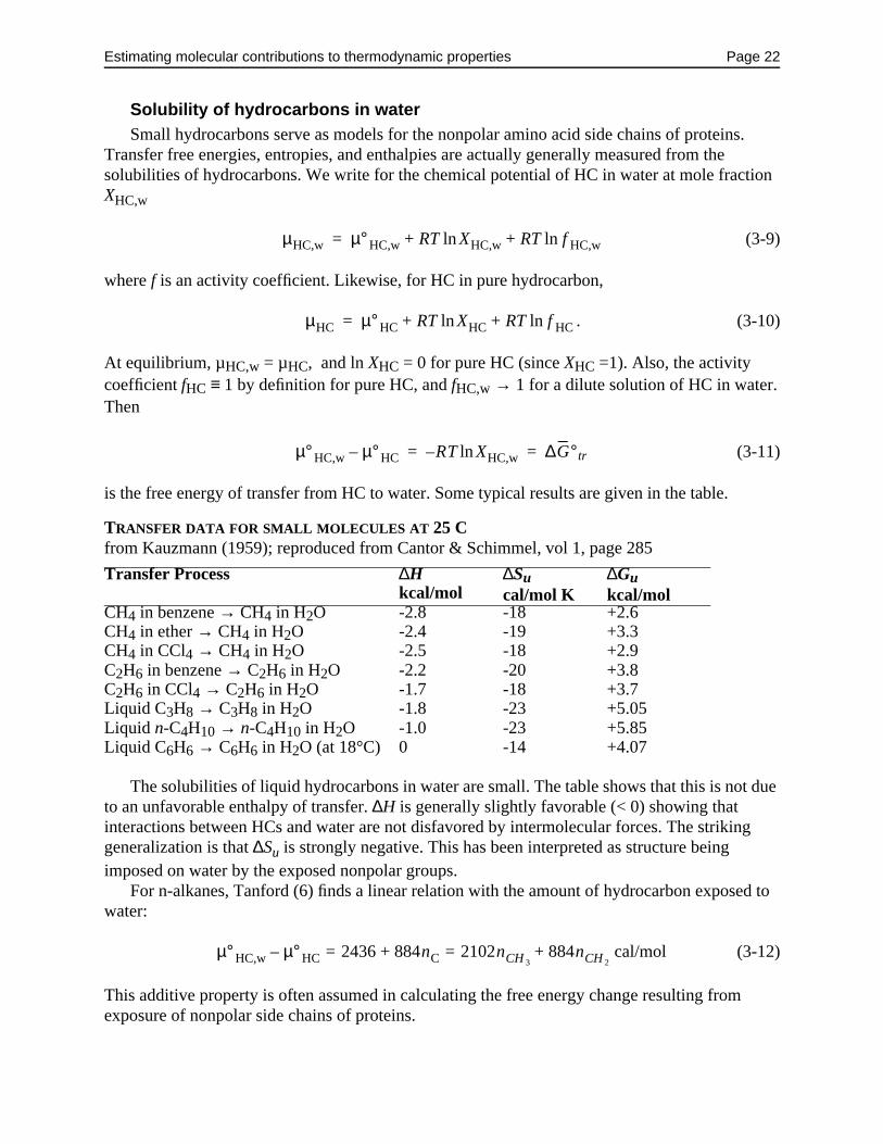
The solubilities of liquid hydrocarbons in water are small. The table shows that this is not due to an unfavorable enthalpy of transfer. ∆H is generally slightly favorable (< 0) showing that interactions between HCs and water are not disfavored by intermolecular forces. The striking generalization is that ∆Su is strongly negative. This has been interpreted as structure being imposed on water by the exposed nonpolar groups.

For n-alkanes, Tanford (6) finds a linear relation with the amount of hydrocarbon exposed to water:

(3-12)

This additive property is often assumed in calculating the free energy change resulting from exposure of nonpolar side chains of proteins.

TRANSFER DATA FOR SMALL MOLECULES AT 25 Cfrom Kauzmann (1959); reproduced from Cantor & Schimmel, vol 1, page 285

Transfer Process ∆Hkcal/mol

∆Sucal/mol K

∆Gukcal/mol

CH4 in benzene → CH4 in H2O -2.8 -18 +2.6CH4 in ether → CH4 in H2O -2.4 -19 +3.3CH4 in CCl4 → CH4 in H2O -2.5 -18 +2.9C2H6 in benzene → C2H6 in H2O -2.2 -20 +3.8C2H6 in CCl4 → C2H6 in H2O -1.7 -18 +3.7Liquid C3H8 → C3H8 in H2O -1.8 -23 +5.05Liquid n-C4H10 → n-C4H10 in H2O -1.0 -23 +5.85Liquid C6H6 → C6H6 in H2O (at 18°C) 0 -14 +4.07

µHC,w µ°HC,w RT XHC,wln RT f HC,wln+ +=

µHC µ°HC RT XHCln RT f HCln+ +=

µ°HC,w µ°HC– R– T XHC,wln ∆G°tr= =

µ°HC,w µ°HC– 2436 884nC+ 2102nCH 3884nCH 2

+= = cal/mol


Hydrophobicity is an effect of the anomalous heat capacity of water exposed to hydrophobic residues.The data tabulated above were obtained at 25 C. More recent experiments over a wide range

of temperature have exposed a more complex reality: ∆H and ∆S are both strongly T-dependent due to large, positive, constant ∆Cp on transferring nonpolar groups from organic solvents to water.

This is evident from the two graphs below. On the left is a model system, the transfer of benzene from organic solvent to water. On the right is denaturation of the protein myoglobin, in which nonpolar amino acid residues are transferred from the nonpolar interior to the aqueous solvent.

In both cases the transfer is unfavorable, but due to unfavorable entropy at low T and to unfavorable enthalpy at high T. Note that ∆S crosses 0 at about 386 K, a general rule proposed by Baldwin (8). Thus the assertion that hydrophobic interactions are entropy-driven is true only under restricted conditions.

Integration of equations for ∆H and ∆S with constant ∆Cp gives

(3-13)

and

(3-14)

which combine to give

(3-15)

∆H° T2( ) ∆H° T1( )= ∆CP° T2 T1–( )+

∆S° T2( ) ∆S° T1( )= ∆CP° T2 T1⁄( )ln+

∆G° T2( ) ∆G° T1( ) ∆CP° T2 T1– T2 T2 T1⁄( )ln+[ ] ∆S° T1( ) T2 T1–( )–+=


Interpretation of large ∆C in terms of fluctuationsIt is a general result from statistical mechanics that CP is related to the fluctuations in internal

energy according to the relation

(3-16)

This implies that when hydrophobic groups are transferred to water, the energy of the water can fluctuate a lot due to choices between structures imposed by hydrophobic groups.

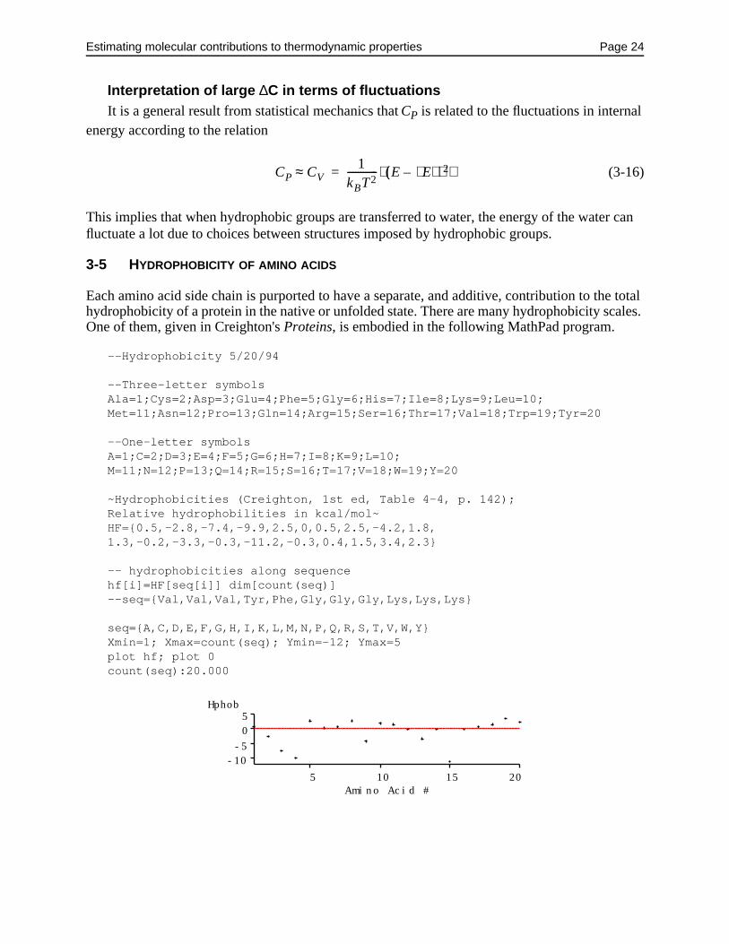
3-5 HYDROPHOBICITY OF AMINO ACIDS

Each amino acid side chain is purported to have a separate, and additive, contribution to the total hydrophobicity of a protein in the native or unfolded state. There are many hydrophobicity scales. One of them, given in Creighton's Proteins, is embodied in the following MathPad program.

--Hydrophobicity 5/20/94

--Three-letter symbolsAla=1;Cys=2;Asp=3;Glu=4;Phe=5;Gly=6;His=7;Ile=8;Lys=9;Leu=10;Met=11;Asn=12;Pro=13;Gln=14;Arg=15;Ser=16;Thr=17;Val=18;Trp=19;Tyr=20

--One-letter symbolsA=1;C=2;D=3;E=4;F=5;G=6;H=7;I=8;K=9;L=10;M=11;N=12;P=13;Q=14;R=15;S=16;T=17;V=18;W=19;Y=20

~Hydrophobicities (Creighton, 1st ed, Table 4-4, p. 142); Relative hydrophobilities in kcal/mol~HF=0.5,-2.8,-7.4,-9.9,2.5,0,0.5,2.5,-4.2,1.8,1.3,-0.2,-3.3,-0.3,-11.2,-0.3,0.4,1.5,3.4,2.3

-- hydrophobicities along sequencehf[i]=HF[seq[i]] dim[count(seq)] --seq=Val,Val,Val,Tyr,Phe,Gly,Gly,Gly,Lys,Lys,Lys

seq=A,C,D,E,F,G,H,I,K,L,M,N,P,Q,R,S,T,V,W,YXmin=1; Xmax=count(seq); Ymin=-12; Ymax=5plot hf; plot 0count(seq):20.000

CP CV≈ 1kBT2------------ E E⟨ ⟩–( )2⟨ ⟩=

5 10 15 20

-10-505

Hphob

Amino Acid #


3-6 ACCESSIBLE SURFACE AREA

Agreement with experiment is more consistent if only the surface area accessible to solvent is counted in hydrophobicity calculations. Accessible surface area is defined as the area traced out by the surface of a probe sphere (usually with radius equal to that of a water molecule) on the surface of the protein (9-10):

3-7 DEPENDENCE OF ∆CP AND ∆S ON NON-POLAR AND POLAR SURFACE AREA

In an important series of papers, Spolar and Record and their associates (11-14) have examined a large number of model systems, and protein and protein-DNA crystal structures, and adduced regularities in the entropy and heat capacity changes associated with exposure of given areas ∆A of both nonpolar (np) and polar (p) surfaces. Their results can be summarized by

(3-17)

and

(3-18)

where A is in Å2 and HE stands for hydrophobic effect. Note that ∆SHE° = 0 at 386 K.

3-8 HYDRATION FORCE

We are increasingly realizing that a significant component of the force between closely approaching macromolecules is due to the water at or near their surfaces (15).

3-9 REFERENCES

1. Hu, C.-Q., J. M. Sturtevant, J. A. Thomson, R. E. Erickson and C. N. Pace. 1992. Thermodynamics of ribonuclease T1 denaturation. Biochemistry. 31: 4876-4882

2. Pace, C. N. 1992. Contribution of the hydrophobic effect to globular protein stability. J. Mol. Biol. 226: 29-35.

Water probe, modelled as 1.4 Å radius sphere

Inaccessible

Interior

Surface

∆CP° 0.32 0.04±( )∆ Anp 0.14 0.04±( )∆ Ap–( ) cal/mol-K=

∆SHE° 0.32∆Anp T 386⁄( )ln=


3. Holtzer, A. (1995). The "cratic correction" and related fallacies. Biopolymers. 35: 595-602.

4. Gilson, M. K., J. A. Given, B. L. Bush & J. A. McCammon. (1997). The statistical-thermodynamic basis for computation of binding affinities: A critical review. Biophys. J. 72: 1047-1069.

5. Murphy, K. P., D. Xie, K. S. Thompson, L. M. Amzel and E. Freire. 1994. Entropy in biological binding processes: Estimation of translational entropy loss. Proteins. 18: 63-67.

6. Tanford, C. (1980). The Hydrophobic Effect: Formation of Micelles and Biological Membranes. New York, John Wiley & Sons.

7. Kauzmann, W. 1959. Some factors in the interpretation of protein denaturation. Adv. Protein Chem. 14: 1-63.

8. Baldwin, R. L. 1986. Temperature dependence of the hydrophobic interaction in protein folding. Proc. Nat. Acad. Sci. USA. 83: 8069-8072.

9. See B.K. Lee and F.M. Richards (1971), J. Mol. Biol. 55: 379-400

10. F.M. Richards (1977), Ann. Rev. Biophys. Bioeng. 6: 151-176.

11. Ha, J.-H., R. S. Spolar and M. T. Record Jr. 1989. Role of the hydrophobic effect in stability of site-specific protein-DNA complexes. J. Mol. Biol. 209: 801-816.

12. Livingstone, J. R., R. S. Spolar and M. T. Record Jr. 1991. Contribution to the thermodynamics of protein folding from the reduction in water-accessible nonpolar surface area. Biochemistry. 30: 4237-4244.

13. Spolar, R. S., J. R. Livingstone and M. T. Record Jr. 1992. Use of liquid hydrocarbon and amide transfer data to estimate contributions to thermodynamic functions of protein folding from the removal of nonpolar and polar surface from water. Biochemistry. 31: 3947-3955.

14. Spolar, R. and M. T. Record Jr. 1994. Coupling of local folding to site-specific binding of proteins to DNA. Science. 263: 777-784.

15. Leikin, S., V. A. Parsegian, D. C. Rau & R. P. Rand. (1993). Hydration forces. Annu. Rev. Phys. Chem. 44: 369-395.

16. Rau, D. C. & V. A. Parsegian. (1992). Direct measurement of temperature-dependent solvation forces between DNA double helices. Biophys. J. 61: 260-271.

17. Rau, D. C. & V. A. Parsegian. (1992). Direct measurement of the intermolecular forces between counterion-condensed DNA double helices. Evidence for long range attractive hydration forces. Biophys. J. 61: 246-259.

Statistical thermodynamics of polymer solutions

4 STATISTICAL THERMODYNAMICS OF POLYMER SOLUTIONS

Proteins and nucleic acids are polymers: large molecules built of many monomeric units covalently attached to each other. Because of their large size, polymers have unusual solution properties relative to small molecules. We discuss in this chapter how polymer size and shape affects the thermodynamic properties of polymer solutions.

4-1 EXCLUDED VOLUME AND VIRIAL EXPANSION

If the volume of the solution is V, and the volume that one molecule of solvent excludes to other molecules is u, then one can use statistical arguments to calculate the number of ways in which N2 molecules of polymer solute can be added to the solution without overlap. This is essentially Ω in the Boltzmann equation S = kB ln Ω. If there is no interaction between polymers other than excluded volume, and no interaction with solvent leading to heat effects, then it can be shown (Tanford, Physical Chemistry of Macromolecules, pp. 192-197) that (neglecting interactions higher than second order)

. (4-1)

Comparing this with eq (2-37) we see that the second virial coefficient B is related to the excluded volume u by

(4-2)

SpheresFor spheres of radius R, the volume excluded by one to the centers of others is

(4-3)

which is eight times the molecular volume, so

(4-4)

where v2 is the specific volume (cc/g) of the polymer. Higher order expansions for spheres will be considered below. It should be noted that random coil polymers are on average spherical, so their second virial coefficient may be estimated from their average radius as defined later in the chapter on polymer conformational statistics.

RodsIndependently Onsager and Zimm showed that for rods of length L and diameter d,

(4-5)

µ1 µ1°– RTV 1°c2

M2-------– 1

NAu

2M2-----------c2+

=

BNAu

2M2-----------=

u4π3

------ 2R( )3=

B 4v2=

u12---πdL2= B→ L

d---v2=


Other repulsive forcesIn addition to the hard sphere and hard rod repulsive forces considered above, electrostatic and

hydration forces may also contribute substantially to B. For highly charged rods, such as DNA, the effect of electrostatics is essentially to increase the diameter d by an amount several times the Debye-Hückel screening radius (1).

Attractive forcesA positive value of B implies repulsion between polymer molecules in solution. A negative

value of B, on the other hand, implies attraction, and is often indicative of association or aggregation.

4-2 DETERMINATION OF MOLECULAR WEIGHT AND SECOND VIRIAL COEFFICIENT FROM OSMOTIC PRESSURE

As noted above, osmotic pressure may be used to measure the molecular weight of a dissolved solute. At the same time, from the concentration dependence of the osmotic pressure, the second virial coefficient may be determined, giving information on molecular size, shape, and interactions. Repeating eq (2-39) here for convenience;

(4-6)

we see that a plot of Π/RTc2 vs c2 has intercept M2 and slope B. In polydisperse solutions, M2 is a number average molecular weight. We'll discuss average molecular weights later.

Osmotic pressure measurements with a semipermeable membrane can be made only within a restricted range of molecular sizes. If the solute is too small, it will not be possible to find a membrane that retains it but not solvent. If the solute is too large, the inverse dependence on M2

means that Π will be too small to measure. Practically, the range of M2 is from about 103 to 105. For smaller molecules, the equivalent colligative property, vapor pressure lowering, can be

measured with a “vapor pressure osmometer”.

4-3 CROWDED SOLUTIONS OF RIGID PARTICLES

When solutions become very crowded, a low-order virial expansion is no longer adequate. A higher order virial expansion can be used. Terms have been worked out to B7 for spheres (2); note that the third virial coeff is B3, not C, in this notation:

. (4-7)

Alternatively, a closed form equation of state can be used (3):

∏RTc2

2c

slope = B

intercept = 1/M2

ΠRTc2

M2------------- 1 Bc2 Cc2

2 …+ + +( )=

ΠM2

c2RT------------- 1 Bic

i 1–

i 2=

7

∑+=


(4-8)

where y = c2v2 is the polymer volume fraction in solution. These two expressions agree very closely, at least up to y = 0.5. (ES = equation of state, VC = virial coefficient expansion)

The MathPad code for these equations is

--Osm press of concentrated solutions 9/26/94

--Equation of state: Carnahan, N. F. & K. E. Starling. (1969). Equation of state for nonattracting rigid spheres, J. Chem. Phys. 51, 635-636.

--Virial coeffs: Ree, F.H. and Hoover, W.G. (1967) J. Chem. Phys. 46: 4181-4197

--y = volume fraction of spherical polymer = vc, v = molec vol, c = molec conc

-- Pi_red = PM/cRT, P = osmotic pressure

--Equation of state:Pi_redES(y) = (1+y+y^2-y^3)/(1-y)^3Xmin=0; Xmax=.5plot Pi_redES(X)

--Virial coeffs:B=4,10,18.36,28.24,39.5,56.4Pi_redVC(y)=1+sum(B[i]*y^i,i,1,count(B))plot Pi_redVC(X)

In semidilute or concentrated solutions where molecular volumes overlap, the thermodynamics approximations of dilute solution theory become increasingly inadequate, as is apparent from the graph above. Biological cells are such concentrated solutions, with volume fractions of more than 0.3 occupied by macromolecules (mainly ribosomes and protein polymers). The thermodynamic consequences of highly crowded solutions have been explored by Minton (4) among others.

ΠM2

c2RT-------------

1 y y2 y3–+ +1 y–( )3

-----------------------------------=

0.0 0.1 0.2 0.3 0.4 0.5

5.0

10.0

Pi_red = ∏M/cRT

y = vc = vol fract

ES

VC


4-4 FLORY-HUGGINS LATTICE THEORY FOR SOLUTIONS OF FLEXIBLE POLYMERS

Up to now we have considered polymers as spheres (which may be considered models for globular proteins) or rods (models for short DNA fragments or protein polymers). These are both rigid structures, fully characterized by one or two dimensional parameters. A third major class of polymer is flexible, and has no fixed size or shape. This is a model for long DNA molecules, or unfolded proteins. It must be treated statistically.

The most widely used statistical thermodynamic treatment is the Flory-Huggins lattice theory (5). In this model, each polymer segment occupies the same volume as a solvent molecule. The lattice has a coordination number (the number of neighbors of each lattice site) of z. The statistical problem of laying down N2 chains, each containing σ monomers, gives the entropy. A sample 2-dimensional configuration is shown in the figure. The result for n1 moles of solvent and n2 moles of polymer chains is

(4-9)

where φ1 and φ2 are the volume fractions (rather than mole fractions) of solvent and solute. Differentiating ∆Smix with respect to n1 yields for the partial molar entropy of the solvent

(4-10)

The enthalpy of mixing is calculated by assuming that the numbers of sites that have 1-1, 1-2,

and 2-2 contacts are proportional to n12, σn1n2, and (σn2)2, respectively; i.e., that there is random

mixing of solvent and polymer. The result is

(4-11)

where

(4-12)

and the ε's are energies of interaction. Differentiating with respect to n1,

(4-13)

Combining the entropy and enthalpy expressions, we get

(4-14)

∆Smix R– n1

n1

n1 σn2+---------------------

ln R– n2

σn2

n1 σn2+---------------------

ln Rn1 φ1ln– Rn2 φ2ln–= =

S1 S1°– R φ1ln– R 11σ---–

φ2–=

∆Hmix n1φ2∆ε=

∆ε NAz12---ε11

12---ε22 ε12–+

=

H1 H1°– ∆εφ22–=

µ1 µ1°– RT 1 φ2–( )ln 1 1σ---–

φ2∆εRT-------φ2

2+ +=


There are two major approximations in the derivations of these equations. One is the assumption of a uniform segment density, which prohibits application to dilute solutions. The other is that the placement of segments is purely random, which cannot be the case if ∆ε is non-zero. ∆ε < 0 will favor clustering of polymer with polymer, and solvent with solvent; ∆ε > 0 will favor mixing of polymer with solvent to an extent greater than statistical. An empirical modification by Flory and Krigbaum treats ∆ε not just as an energy term, but as containing both energy and entropy contributions. They obtain an expression that sets

(4-15)

where ψ is an entropy parameter and Θ is a temperature, the so-called "theta temperature". When T = Θ, the theory predicts that a very long polymer, σ → ∞, is just on the verge of precipitating out of solution. That is, Θ marks a transition between "good solvent" at higher T and "poor solvent" at lower T. For a chain at the Θ-temperature, the second virial coefficient B = 0.

The lattice model of polymer solutions has been used recently, especially by Ken Dill and co-workers, to model protein folding. They use exhaustive computer enumeration to find all the chain conformations of relatively short polypeptide chains, σ ≤ 16 or so, and to impose a ∆ε between segments designated as hydrophobic.

4-5 REFERENCES

1. Stigter, D. (1977). Interactions of highly charged colloidal cylinders with applications to double-stranded DNA, Biopolymers 16, 1435-1448.

2. Ree, F.H. and Hoover, W.G. (1967) J. Chem. Phys. 46: 4181-4197.

3. Carnahan, N. F. & K. E. Starling. (1969). Equation of state for nonattracting rigid spheres, J. Chem. Phys. 51, 635-636.

4. Minton, A. P. (1983). The effect of volume occupancy upon the thermodynamic activity of proteins: Some biochemical consequences, Molec. & Cell. Biochem. 55, 119-140.

5. Flory, P.J. (1953) Principles of Polymer Chemistry, Cornell University Press, Ithaca, New York. Chapter XII.

6. Dill, K. A., S. Bromberg, K. Yue, K. M. Fiebig, D. P. Yee, P. D. Thomas & H. S. Chan. (1995). Principles of protein folding--A perspective from simple exact models. Protein Sci. 4: 561-602.

12---

∆εRT-------– ψ 1

ΘT----–

=

part i. thermodynamics and statistical thermodynamicsaathavan/libraire/thermodynamicspri… · part...

Documents