Chapter 3pGlobal Flow Regimes

Gl b l Fl R iGlobal Flow Regimes• At any given time in the producing life of a

reservoir, the fluid flow condition existing may be characterized as eithery

a) transient, b) pse dostead state orb) pseudosteady-state or c) steady-state.

• What do these terms mean?

R i FlReservoir Flow

• Initially, in a virgin reservoir, the pressure at any fixed depth is constant.As production begins the pressure near the• As production begins, the pressure near the wellbore drops significantly as near-wellbore fluids expand to satisfy the imposed production condition.

• Far away from the well, no measurable pressure drop can be observed at early timespressure drop can be observed at early times – locations far away from the well are not

“aware” that the reservoir is being produced.

TransientTransient• As time progresses, pressure drops can be

meas red f rther and f rther a a from themeasured further and further away from the well, an increasing volume of the reservoir fluids expand to contribute to the well's production.

• During this period, the reservoir is said to be “infinite acting” and the flow is transient;infinite acting and the flow is transient; pressure drop at outer reservoir boundary is negligible.

• The pressure versus time behavior at the producing wellbore contains information about the reservoir permeability.p y

P d t d St tPseudosteady State• After a long time pressure drops can be• After a long time, pressure drops can be

measured at all reservoir locations– the entire reservoir is contributing to the g

well's production. • At this time, the pressure changes at the

same rate at every location in the reservoirsame rate at every location in the reservoir, i.e., dp(x,t)/dt = constant; pseudosteady state flow.

• The pressure versus time behavior at the wellbore reflects the volume of fluid (or the reservoir pore volume) contributing toreservoir pore volume) contributing to production.

Steady Statey• To see steady-state flow in a reservoir, we must

replace reservoir fluids at the same rate that we thremove them.

• This situation may occur if we have a recharge toThis situation may occur if we have a recharge to the system (an assocaited water aquifer) or may also occur in secondary and enhanced oil recovery operations e g waterflooding gasrecovery operations - e.g., waterflooding, gas injection, etc.

• During steady-state single-phase flow, nothing is changing in the reservoir, i.e., dp(x,t)/dt = 0. Note there is a pressure drop in the reservoir, andthere is a pressure drop in the reservoir, and pressure data contains information about recharging system parameters.

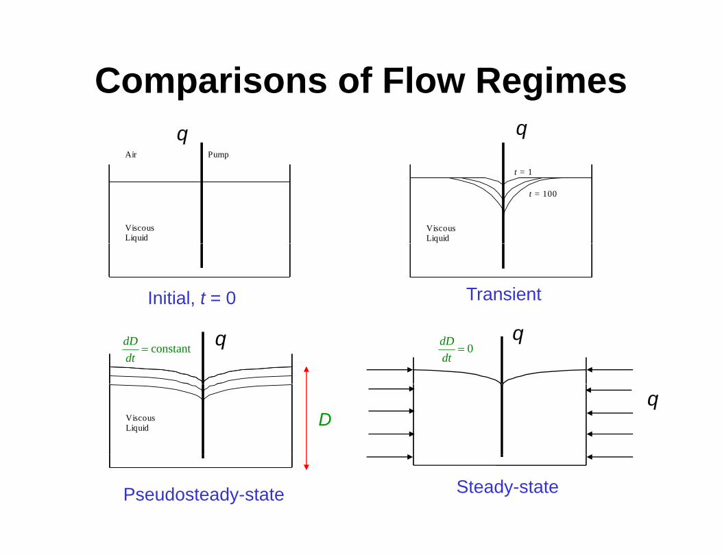
Comparisons of Flow Regimes

PumpAir

t = 1

q q

ViscousLiquid

ViscousLiquid

t 1

t = 100

Initial, t = 0 Transient

constantdDdt

=qq 0dD

dt=

ViscousLiquid

qD

Pseudosteady-state Steady-state

D ’ LDarcy’s Law

• For flow through a horizontal sand pack, flow rate is– Directly proportional to the pressure drop

across the packDirectl proportional to the (gross) area– Directly proportional to the (gross) area open to flow

– Inversely proportional to the length of theInversely proportional to the length of the pack

– Inversely proportional to fluid viscosityy p p y• Constant of proportion is the “permeability”

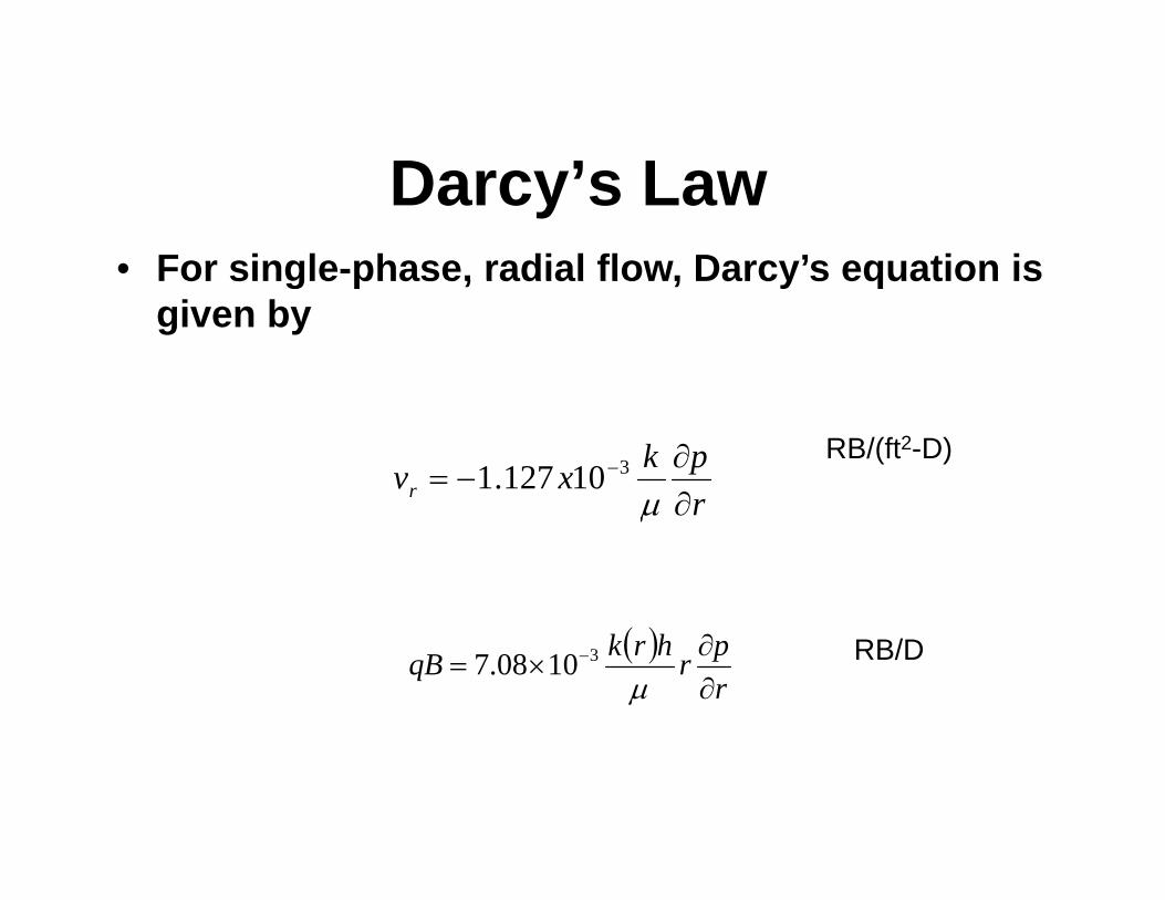
D ’ LDarcy’s Law• For single-phase, radial flow, Darcy’s equation isFor single phase, radial flow, Darcy s equation is

given by

rpkxvr ∂∂

−= −

μ310127.1

RB/(ft2-D)

r∂μ

( )rprhrkqB∂∂

×= −

μ31008.7 RB/D

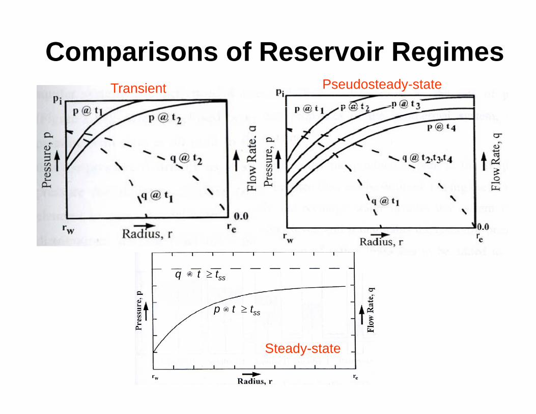
Comparisons of Reservoir RegimesTransient Pseudosteady-state

t ≥ tssq

t ≥ tssp

Steady-state

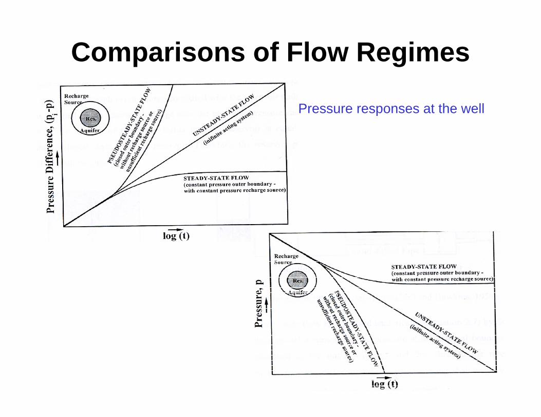
Comparisons of Flow Regimes

Pressure responses at the well

Steady-State Radial FlowSteady-State Radial Flow

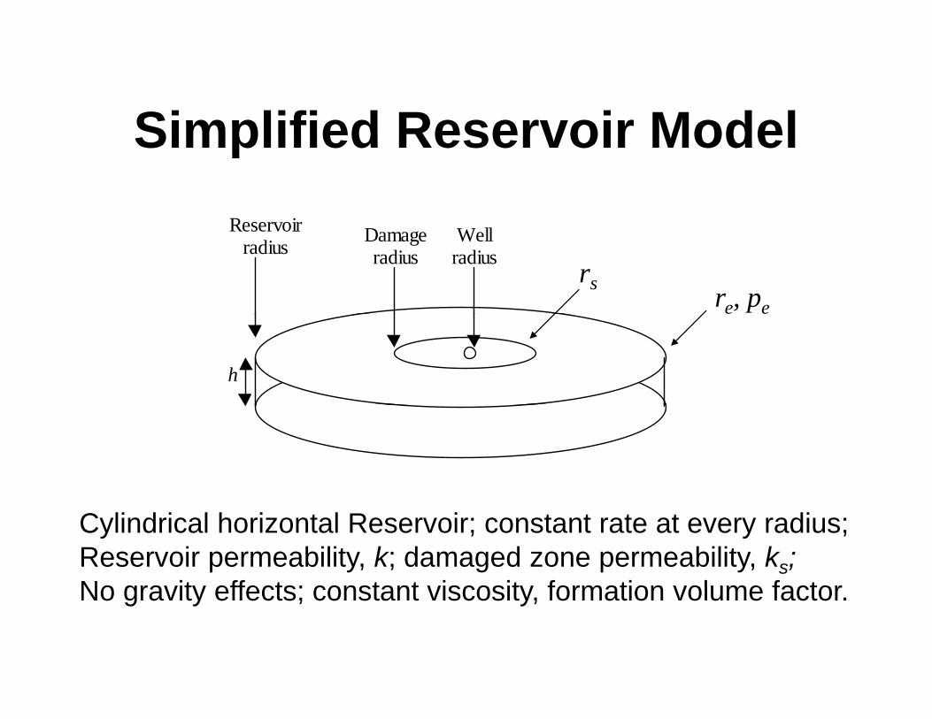
Simplified Reservoir ModelSimplified Reservoir ModelReservoirReservoir

radius Damageradius

Wellradius rs re, pe

h

Cylindrical horizontal Reservoir; constant rate at every radius;Reservoir permeability, k; damaged zone permeability, ks;No gravity effects; constant viscosity formation volume factorNo gravity effects; constant viscosity, formation volume factor.

D ’ LDarcy’s Law

• Rate at any radius:( ) phrkB ∂−310087

• Pressure distribution

( )rprqB∂

×=μ

31008.7

• Pressure distribution– Integrate Darcy’s law over radius

O t ( d d )– Outer (undamaged zone)

∫∫ =× −ee rp drdpkh310087

( )∫∫ =×rrp r

dpqBμ

1008.7

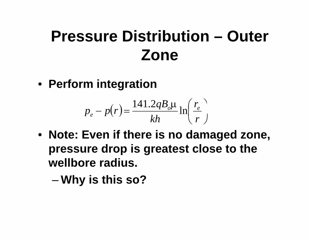
Pressure Distribution – Outer Zone

• Perform integration

( ) ⎞⎛μ rqB2141

• Note: Even if there is no damaged zone

( ) ⎟⎠⎞

⎜⎝⎛μ

=−rr

khqBrpp eo

e ln2.141

• Note: Even if there is no damaged zone, pressure drop is greatest close to the wellbore radiuswellbore radius.– Why is this so?

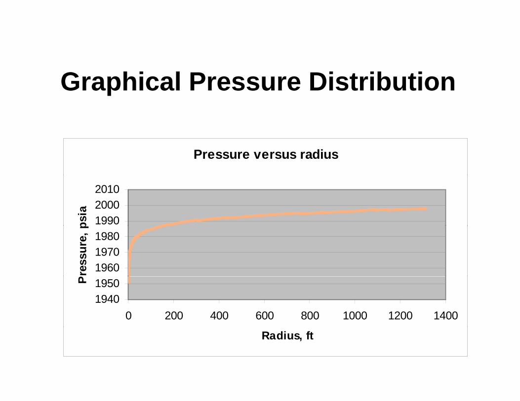
G hi l P Di t ib tiGraphical Pressure Distribution

Pressure versus radius

199020002010

psia

196019701980

ress

ure,

p

19401950

0 200 400 600 800 1000 1200 1400

P

Radius, ft

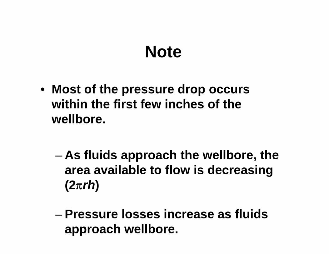
N tNote

• Most of the pressure drop occurs within the first few inches of the wellbore.

– As fluids approach the wellbore, the area available to flow is decreasing g(2πrh)

– Pressure losses increase as fluids approach wellbore.

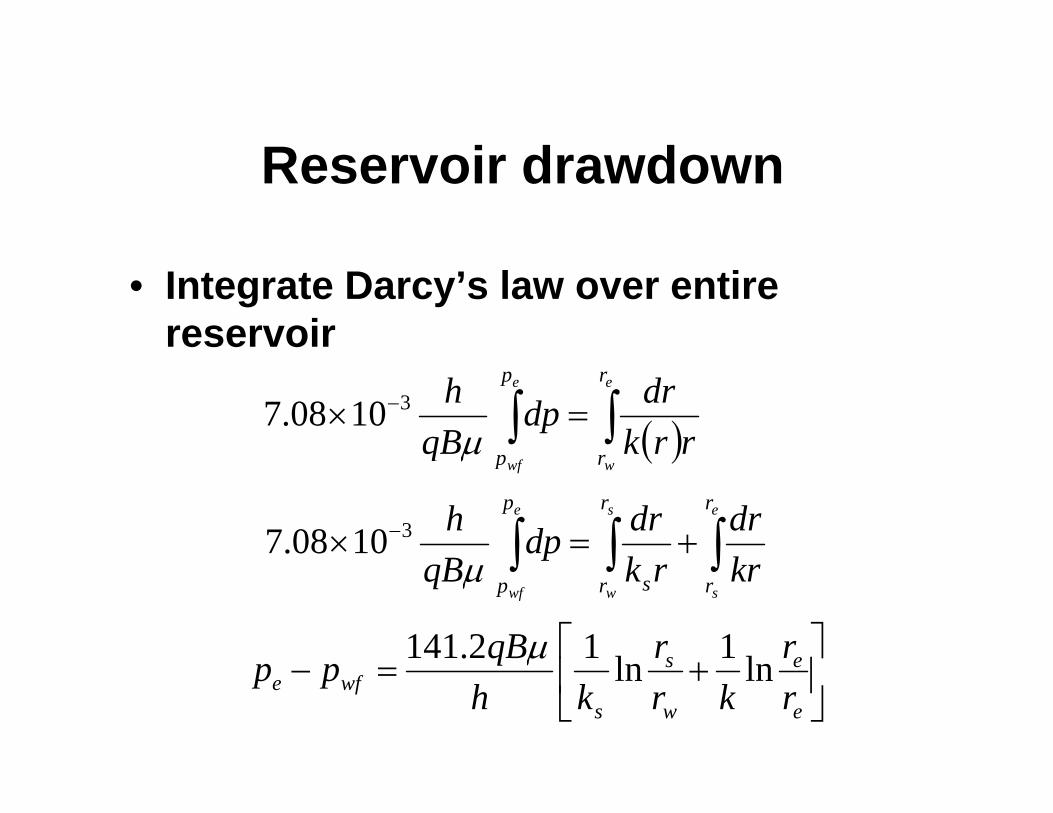
R i d dReservoir drawdown

• Integrate Darcy’s law over entire reservoir

( )∫∫ =× −ee r

r

p

p rrkdrdp

qBhμ

31008.7 ( )wwf rpq μ

∫∫∫ +=× −ese rrp

kdr

kdrdp

Bh31008.7 ∫∫∫

swwf rr sp krrkp

qBμ

⎥⎤

⎢⎡

+ es rrqB l1l12.141 μ⎥⎦

⎢⎣

+=−e

e

w

s

swfe rkrkh

qpp lnlnμ

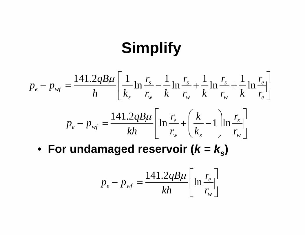
Si lifSimplify

⎤⎡⎥⎦

⎤⎢⎣

⎡++−=−

e

e

w

s

w

s

w

s

swfe r

rkr

rkr

rkr

rkh

qBpp ln1ln1ln1ln12.141 μ

⎥⎦

⎤⎢⎣

⎡⎟⎟⎠

⎞⎜⎜⎝

⎛−+=− se

wfe rr

kk

rr

khqBpp ln1ln2.141 μ

• For undamaged reservoir (k = ks)⎦⎣ ⎠⎝ wsw rkrkh

⎥⎦

⎤⎢⎣

⎡=− e

wfe rr

khqBpp ln2.141 μ

⎦⎣ wrkh

Ski F tSkin Factor

• Define skin factor, s, as

srk l1⎟⎞

⎜⎛

• Skin factor isw

s

s rks ln1⎟⎟

⎠⎜⎜⎝

−=

– A dimensionless number– = 0 if there is no damage– > 0 if there is damage– < 0 if the near-wellbore region is

ti l t dstimulated

P d ti it I dProductivity Index

• For steady state flow

( ) ==khqJ ( )

⎟⎟⎠

⎞⎜⎜⎝

⎛+⎟⎟⎠

⎞⎜⎜⎝

⎛μ

=−

=

srrB

ppJ

w

ewfeo

ln2.141

– A positive skin factor will reduce the well’s productivityA ti ki ill i it– A negative skin will increase it

– Are there any other factors that influence a well’s productivity?well s productivity?

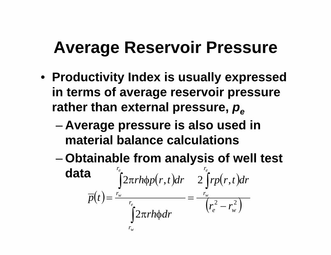
Average Reservoir PressureAverage Reservoir Pressure• Productivity Index is usually expressedProductivity Index is usually expressed

in terms of average reservoir pressure rather than external pressure, pep , pe

– Average pressure is also used in material balance calculationsmaterial balance calculations

– Obtainable from analysis of well test data ( ) ( )

rr

ddhee

φ ∫∫data

( )( ) ( )

( )22

,2,2r

rr

rr

drtrrpdrtrprhtp w

e

w

−=

φπ

=∫

∫

∫( )

2 we

r

rrdrrh

w

φπ∫

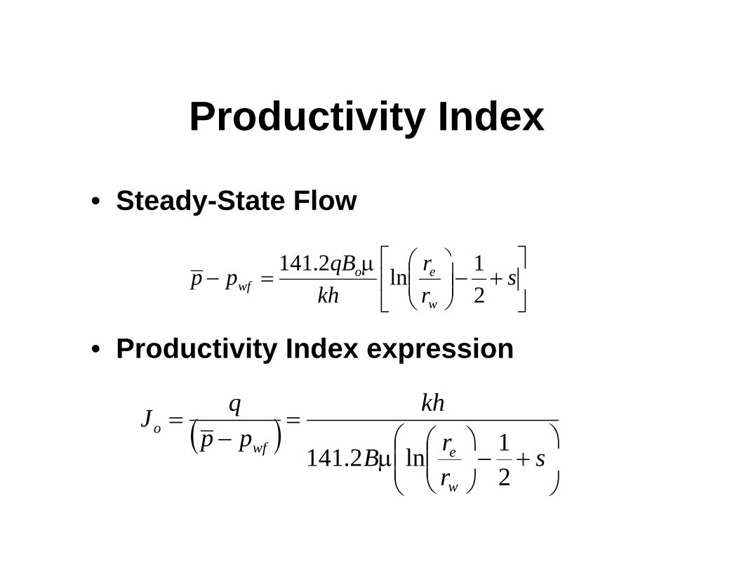
P d ti it I dProductivity Index

• Steady-State Flow

⎤⎡ ⎞⎛⎥⎦

⎤⎢⎣

⎡+−⎟⎟

⎠

⎞⎜⎜⎝

⎛μ=− s

rr

khqBpp

w

eowf 2

1ln2.141

• Productivity Index expression

kh( )

⎟⎟⎞

⎜⎜⎛

+−⎟⎟⎞

⎜⎜⎛

μ

=−

=

srB

khpp

qJewf

o1ln2.141 ⎟

⎠⎜⎝

+⎟⎟⎠

⎜⎜⎝

μ sr

Bw 2

ln2.141

N tNotes

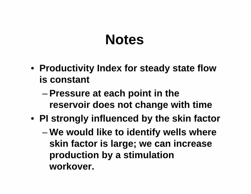
• Productivity Index for steady state flow is constant– Pressure at each point in the

reservoir does not change with timeg• PI strongly influenced by the skin factor

– We would like to identify wells whereWe would like to identify wells where skin factor is large; we can increase production by a stimulation p oduct o by a st u at oworkover.

SkiSkin

• In practice, skin may be due to a variety of factors– Damage to formation due to invasion of

mud filtrate and mud solidsPartial penetration– Partial penetration

– Migration of finesAsphaltines– Asphaltines

• Treatment of skin will depend on the specific cause.cause.

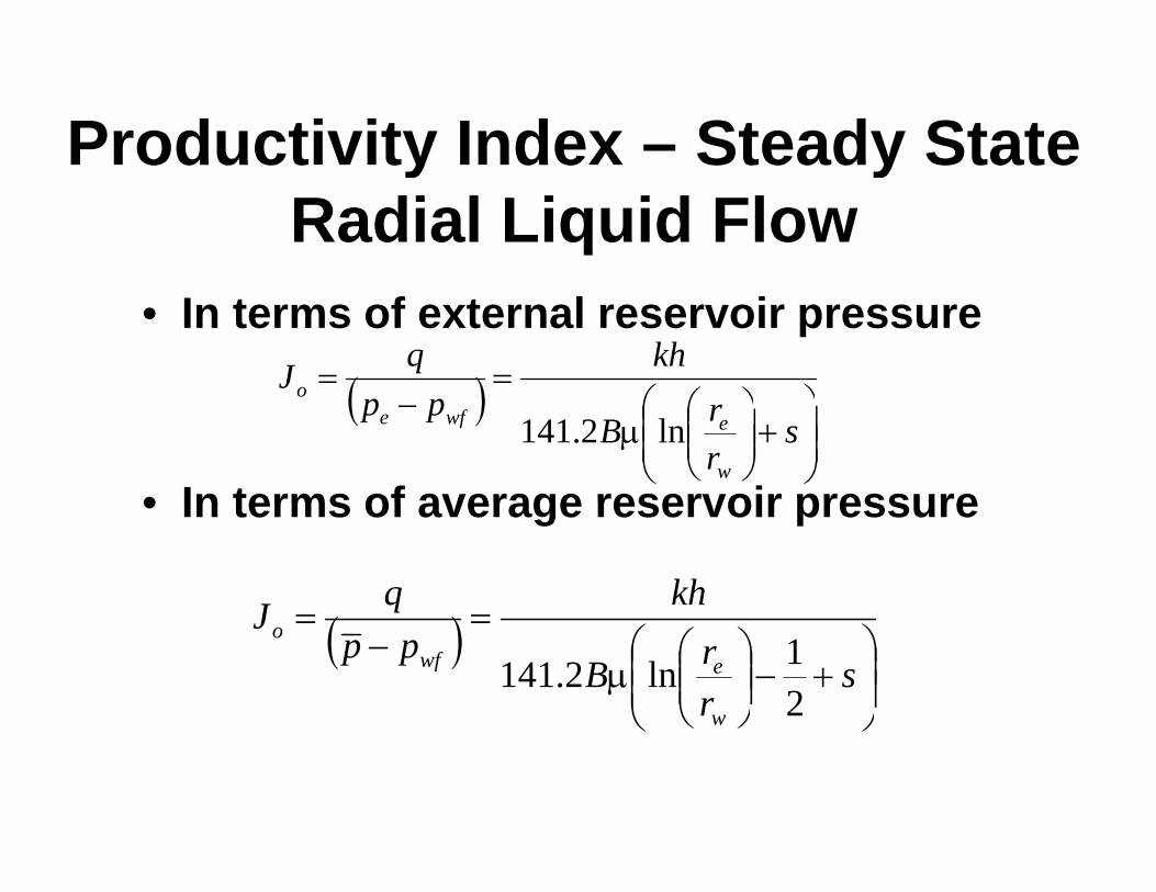
Productivity Index – Steady State oduct ty de Steady StateRadial Liquid Flow

• In terms of external reservoir pressure

( ) ⎞⎛ ⎞⎛==

khqJo

• In terms of average reservoir pressure

( )⎟⎟⎠

⎞⎜⎜⎝

⎛+⎟⎟⎠

⎞⎜⎜⎝

⎛μ

−s

rrB

pp

w

ewfeo

ln2.141

• In terms of average reservoir pressure

==khqJ ( )

⎟⎟⎠

⎞⎜⎜⎝

⎛+−⎟⎟

⎠

⎞⎜⎜⎝

⎛μ

=−

=

srrB

ppJ

w

ewfo

21ln2.141

⎠⎝ ⎠⎝

Pseudosteady State Radial Liquid Flow

A l ti TAccumulation Term

• During pseudosteady state flow,

( )∂ trp

• Reservoir flow equation for pseudosteady

( ) constant,==

∂∂ A

ttrp

state

pk⎟⎞

⎜⎛ ∂∂006330 Ac

rpkr

rr tφ=⎟⎟⎠

⎞⎜⎜⎝

⎛∂∂

μ∂∂00633.0

B d C ditiBoundary Conditions

• The previous differential equation is secondorder; we need two boundary conditions

• In addition we have an unknown constant, A– Outer boundary sealed:

I b d t t t t

0=∂∂

errp

– Inner boundary at constant rate:

( )31.127 10 2 k prh qBr

πμ

−⎡ ⎤∂× =⎢ ⎥∂⎣ ⎦

wrrμ ∂⎣ ⎦

D t i ti f C t t ADetermination of Constant A

• Integrate flow equation over reservoir

φ=⎟⎟⎞

⎜⎜⎛ ∂∂

∫∫006330rr

rdrAcdrpkree

⎟⎟⎞

⎜⎜⎛ −φ∂∂

φ=⎟⎟⎠

⎜⎜⎝ ∂μ∂ ∫∫00633.0

22wet

rt

r

rrAcpkrpkr

rdrAcdrr

rr

ww

• Inner boundary condition

⎟⎟⎠

⎜⎜⎝

=∂μ

−∂μ 200633.0

wet

rr rr

rr

we

( )31.127 10 2k p qBr

r hμ π−

⎡ ⎤∂=⎢ ⎥∂ ×⎣ ⎦ ( )1.127 10 2

wrr hμ π∂ ×⎣ ⎦

Rate of Change of Pressure with ate o C a ge o essu e ttime

• Solve for A2 2c A r r qBφ ⎛ ⎞−

( )30.00633 2 1.127 10 25 615

t e wc A r r qBh

p qB

φπ−

⎛ ⎞−=−⎜ ⎟ ×⎝ ⎠

∂

( )2 2

5.615

e w t

p qBAt h r r cπ φ∂

= =−∂ −

• During pseudo-steady state flow, pressure is a linear function of time; slope inversely proportional to pore volumeproportional to pore volume.

P d ti it I dProductivity Index

• Pseudosteady State Flow

( ) 1fkh p p r− ⎛ ⎞

• If skin were included

( ) 1ln141.2 2

e wf e

w

kh p p rqB rμ

⎛ ⎞= −⎜ ⎟

⎝ ⎠

( ) 1lne wf ekh p p r s

− ⎛ ⎞= − +⎜ ⎟ln

141.2 2w

sqB rμ

+⎜ ⎟⎝ ⎠

( )q khJ = =

⎛ ⎞⎛ ⎞( ) 1141.2 ln2

e wf e

w

p p rB sr

μ⎛ ⎞− ⎛ ⎞

− +⎜ ⎟⎜ ⎟⎜ ⎟⎝ ⎠⎝ ⎠

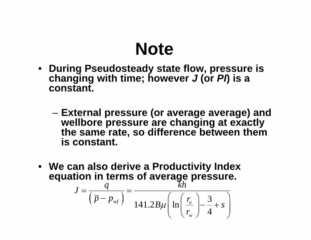
N tNote• During Pseudosteady state flow, pressure is

h i ith ti h J ( PI) ichanging with time; however J (or PI) is a constant.

– External pressure (or average average) and wellbore pressure are changing at exactly the same rate, so difference between themthe same rate, so difference between them is constant.

• We can also derive a Productivity Index• We can also derive a Productivity Index equation in terms of average pressure.

( ) 3q khJ = =

⎛ ⎞⎛ ⎞( ) 3141.2 ln4

wf e

w

p p rB sr

μ⎛ ⎞− ⎛ ⎞

− +⎜ ⎟⎜ ⎟⎜ ⎟⎝ ⎠⎝ ⎠

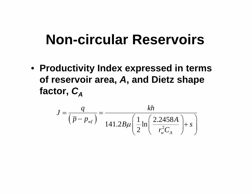
N i l R iNon-circular Reservoirs

• Productivity Index expressed in terms of reservoir area, A, and Dietz shape factor, CA

q kh( )

21 2.2458141.2 ln2

wf

w A

q khJp p AB s

r Cμ

= =⎛ ⎞− ⎛ ⎞

+⎜ ⎟⎜ ⎟⎜ ⎟⎝ ⎠⎝ ⎠w A⎝ ⎠⎝ ⎠

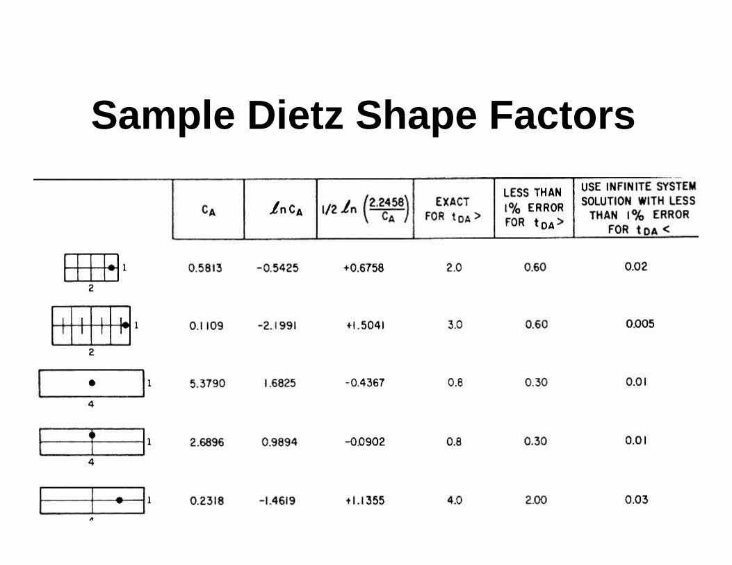
S l Di t Sh F tSample Dietz Shape Factors

Transient FlowTransient Flow• Transient Flow includes a set of transientTransient Flow includes a set of transient

flow regimes

– Wellbore storage dominated flow– Spherical flow

Radial Flow– Radial Flow– Linear Flow– etcetc

• These are all subsets of an overall transient flow regime

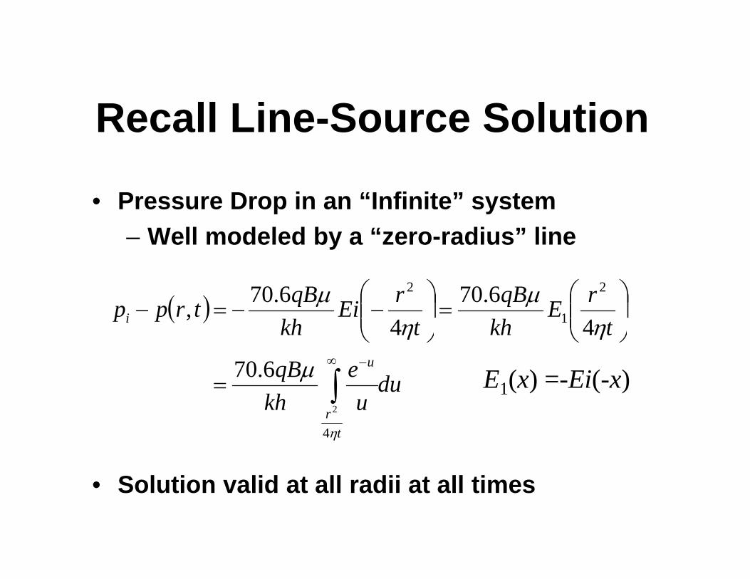
R ll Li S S l tiRecall Line-Source Solution

• Pressure Drop in an “Infinite” system– Well modeled by a “zero-radius” line

( )t

rEkhqB

trEi

khqBtrppi ⎟⎟

⎠

⎞⎜⎜⎝

⎛=⎟⎟

⎠

⎞⎜⎜⎝

⎛−−=−

ημ

ημ 2

1

2

46.70

46.70,

duekhqB

tkhtkhu

∫∞ −

=

⎟⎠

⎜⎝

⎟⎠

⎜⎝

μ

ηη

6.70

44

E1(x) =-Ei(-x)ukh

tr∫η4

2

• Solution valid at all radii at all times

T i t P d ti it I dTransient Productivity Index

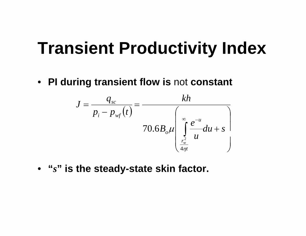
• PI during transient flow is not constant khqJ sc

( )

⎟⎟⎟⎞

⎜⎜⎜⎛

+

=−

=

∫∞ −

sdueB

tppqJ

u

o

wfi

sc

μ6.70⎟⎟⎠

⎜⎜⎝

∫ ut

ro

w

η

μ

4

2

• “s” is the steady-state skin factor.