part 2: anniversary supplement || some computation-steeples in fluid mechanics

Some Computation-Steeples in Fluid MechanicsAuthor(s): W. F. AmesSource: SIAM Review, Vol. 15, No. 2, Part 2: Anniversary Supplement (Apr., 1973), pp. 524-552Published by: Society for Industrial and Applied MathematicsStable URL: http://www.jstor.org/stable/2028683 .

Accessed: 18/06/2014 02:45

Your use of the JSTOR archive indicates your acceptance of the Terms & Conditions of Use, available at .http://www.jstor.org/page/info/about/policies/terms.jsp

.JSTOR is a not-for-profit service that helps scholars, researchers, and students discover, use, and build upon a wide range ofcontent in a trusted digital archive. We use information technology and tools to increase productivity and facilitate new formsof scholarship. For more information about JSTOR, please contact [email protected].

.

Society for Industrial and Applied Mathematics is collaborating with JSTOR to digitize, preserve and extendaccess to SIAM Review.

http://www.jstor.org

This content downloaded from 188.72.126.108 on Wed, 18 Jun 2014 02:45:30 AMAll use subject to JSTOR Terms and Conditions

http://www.jstor.org/action/showPublisher?publisherCode=siam

http://www.jstor.org/stable/2028683?origin=JSTOR-pdf

http://www.jstor.org/page/info/about/policies/terms.jsp


SIAM REVIEW Vol. 15, No. 2, April 1973 Part 2 of two parts Anniversary Supplement

SOME COMPUTATION-STEEPLES IN FLUID MECHANICS*

W. F. AMESt

Abstract. Contained herein is a survey of recent developments in numerical methods for solving the nonlinear equations of fluid mechanics. Strictly numerical methods for integrating these nonlinear models for fluid flow arise from three general formulations: (a) stream function and vorticity, (b) primitive variables, (c) vector potential. An additional section discusses some possible alternatives.

TABLE OF CONTENTS

1. Introduction 524 2. Stream function and vorticity formulation 525 3. Primitive variable formulation 529 4. Vector potential formulation 533 5. New directions 539

5.1. Predictor-corrector methods 540 5.2. Exact difference procedures 541 5.3. Finite elements 544 5.4. New variables 547 References 549

Mechanics is the paradise of the mathematical sciences, because by means of it one comes to the fruits of mathematics. Therefore 0 students study mathematics, and do not build without foundations.-

LEONARDO DA VINCI

1. Introduction. After accepting the praise and noting that the advice is usually followed in theoretical developments, it is startling to observe how often it is ignored in the computational phase of mechanics. Undoubtedly this results from the immense volume of literature produced during the period 1951-1971. An updated and supplemented literature survey on numerical methods for partial differential equations has been compiled by Giese [31]. Of the more than 8,000 separate entries over 2,000 concern various computational aspects of fluid mechanics! At first glance there seems to be as many numerical methods as problems. This is probably true in the details but the historical development lists three general formulations, stream function and vorticity, primitive variables and vector potential to which various computational algorithms have been applied. The essential nonlinearities complicate both the analysis and computation.

Before the era of the third generation computing machines (early 1960's) numerical computations in fluid mechanics, wherein the nonlinearities are retained, are very limited in number. One due to Thom [65] in 1933 studied the wake associated with steady laminar flow past a circular cylinder. Solutions were obtained on a desk calculator for Reynolds numbers ten and twenty. Flugge-Lotz and her students (cf. Ames [3, pp. 349-355]) have carried on extensive calculations of boundary layer flow since the early 1950's. That period also saw advances in our ability to compute gas flows. To be particularly noted is the work of Lax and his

*Received by the editors August 11, 1972. Presented by invitation at the Symposium on Continuum Mechanics, supported in part by the National Science Foundation, at the 20th Anniversary Meeting of the Society for Industrial and Applied Mathematics, held in Philadelphia, Pennsylvania, June 12-14, 1972.

t Department of Mechanics and Hydraulics, University of Iowa, Iowa City, Iowa 52240.

524



COMPUTATION-STEEPLES IN FLUID MECHANICS 525

students (cf. Ames [3, p. 445]). Herein, we shall not repeat the discussions available in other references (e.g., Richtmyer and Morton [59], Ames [3], [4]) but will primarily confine our attention to the numerical methods developed in the last few years for solving the nonlinear equations of fluid mechanics.

2. Stream-function and vorticity techniques. This first group of numerical methods has the common feature that the stream function and vorticity are used as the dependent variables. The equations modeling the time-dependent flow of a two-dimensional viscous incompressible Newtonian fluid in Cartesian coordinates are those of momentum (Navier-Stokes)

(2.1) Ut + uux + vuy = -p' Px + v(uxx + uyy)

(2.2) vt + uvx + vvy = -p 'p + v(vxx + vyy)

and continuity

(2.3) uX + vy = 0.

The dependent variables are the velocity components u and v in the x and y directions, respectively, and the pressure p. The kinematic viscosity, v, and the density, p, are material constants. A stream function i and vorticity co are defined by means of the relations

(2.4) u = iy, v = -x, = -uy + vX,

whereupon we find one form of the vorticity equation'

(2.5) wt)t + (Uw_))x + (Vw_))y = VV2%.

An alternative form of (2.5) is

(2.6) t)t + OOX - Oy = VV20.

We also note that the definition of co (see (2.4)) may be written in terms of i as (2.7) = -a).

A knowledge of the pressure is often useful as an aid in understanding features of the flow. A suitable pressure equation is found by computing the x derivative of (2.1), the y derivative of (2.2) and summing the results. This generates

(2.8) V2p = -p[(u2)xx + 2(uv)xy + (V2)yy].

Probably Emmons [26] was the first author to use the stream function and vorticity method in a digital computer calculation. He was concerned with the numerical solution of (2.6) and (2.7), at a Reynolds number of 4000, with the goal of understanding turbulence. His explicit finite difference discretization employs a forward difference in time and a standard five-point molecule for each Laplacian. Later Payne [53] employs essentially the same ideas in his calculation of nonsteady flow. In particular Payne applies his method to the calculation of wake structure behind a circular cylinder.

1 We shall use V2 to denote the Laplace operator in the appropriate coordinate system.



526 W. F. AMES

Fromm [29], [30], building on the ideas of the preceding investigators, prefers to discretize u = y v = - 0_i and (2.5) and (2.7). He maintains the structure of (2.5) since the velocity components are always of interest and (2.5) is simpler than (2.6). With Ax = Ay = a we use the notation _wn = O(ia,ja, nAt). The vorticity equation (2.5) is discretized with a time-centered scheme wherein the diffusion terms wt = VV2Co) are approximated by a DuFort and Frankel [25] molecule

n+1 ni 2vAt 2&1-2 C9 -w = a20{ j + w,-11j + (i - 0 ij 7 - }.

(2.9)

Equation (2.9) is known to be unconditionally stable for the diffusion equation but does not always satisfy the consistency condition (cf., e.g. Richtmyer and Morton [59] or Ames [4]). The final algorithm for advancing the vorticity to a new time is the explicit scheme

Mt+1 1

0 1 + 4vAt/a 2{"

2At V + [(UO))7- 1/2,j - (UO)I+ 1/2,j + (vi)j -1/2 (VO)7i,J+ 1/2] a (2.10) 2A

+ a2 [w_)n+ 1,j + C9i- L1j + _9n + _n

Velocities and vorticities required by the calculation are obtained by averaging over the values specified at the nearest points in accordance with the relations

(2.11) Ui- 1/2,j = 4(Ui- lj+ 1/2 + Ui- 1,j- 1/2 + Ui,j+ 1/2 + Ui,j- 1/2),

(2.12) Vij-112 = 4(Vi- 12,j + Vi+112,j + Vi-112,j-1 + Vi+112,j-1),

(2.13) (D)i 1/2,j = 2(0)i-l,j + e)ij),

and the remaining quantities in (2.10) are obtained by a suitable permutation of the indices. For the first time advancement Fromm takes wo' = wO. While vorticities on an obstacle are not changed at this stage special consideration is given to the boundary values, particularly in the case of containing walls. For computation at the wall, with fluid below the wall, we use

n = 1+ 1 nK' 2At U 1 + 4vAt/a2 L' ,j + a2 [(U)i- 1/2,jo- (uw)i + 1/2,jo + (v) 1/2]

2vAt2w '} + a2 [wt)i+ 'Jo + Ct)i-l,Jo + Ct)isjo + Ct)i,jo - Jo

where jo is the y index for the upper wall. If the wall velocity is uo, then (2.11) becomes

Ui- 1/2,jo =[2uo+ Ui -l,jo- 1/2 + Uijo- 1/2].

Similar boundary treatment occurs for fluid above a wall.




Without viscosity and when a time centered difference is used a restriction must be imposed on At for stability of (2.10). However, with diffusion only, the difference form requires no restriction on At. Experience (Harlow [33]) indicates that conditions for achieving accuracy of solution of stable equations are very nearly the same as stability criteria for corresponding (possibly) unstable equations. Consequently the two conditions

(2.14) ~~luol + Ivol At<1 vAt <1 (2.14) ?+?At ? 1, 2- a a2 =4 were imposed.

Once the vorticity field is advanced to the (n + l)st time value the advanced field values for A are obtained by a Gauss-Seidel iteration through the application2 of

(2.15) = *{Vi+, + 1i,) + Vp4+1 + O,Pj- ) + a _)i,j}

While Fromm did not use an acceleration technique it seems clear that one such as successive overrelaxation (cf., e.g., Ames [4]) should be used. Values of tr on an obstacle are taken as the reference value I/Jr while wall values are obtained by averaging the individual values. For fluid above a wall, since the wall must contain a streamline,

(2.16) o = 01-uoa + a2coo.

When the / field has converged sufficiently, as determined by some criteria, the new velocities are calculated by means of

un +1 I ij-1/2

=a

Vi- 1/2 ,i a{ i-1 ,j oi,j }

and the vorticity values are brought up to the (n + 1)st time by applying the definition (equation (2.4))

0f+1 = {Uij2

- Ui,j+1/2 + Vi+112,j- Vi-112,jl

At walls the vorticity values are modified to conform to the / field locally. At the lower wall we simply solve (2.16) for co0. The process is then repeated.

Harlow and Fromm [34] have used essentially the same method for the two-dimensional problem of heat transfer from a rectangular cylinder into a surrounding fluid. Wilkes [71] solved the thermal convection problem in a two- dimensional cell essentially using an alternating direction implicit procedure (e.g. Ames [4]). Though the method is unconditionally stable for the linear diffusion equation, Wilkes found it to be unstable for his nonlinear problem at a Grashof

2 The p superscript indicates the iteration step at the (n + l)st time. It should not be confused with the time index. The co's are the advanced values.



528 W. F. AMES

number of 200,000.3 Pearson [54] solved the unsteady, axisymmetric viscous flow generated by the differential rotation of two infinite parallel disks using an adapta- tion of the Crank-Nicolson centered scheme (cf., e.g. Ames [4]) for the vorticity transport equation (2.6). The resulting algebraic problem was solved by successive overrelaxation when the flow was almost linear or by a modified alternating direction implicit method (ADI) of Peaceman and Rachford when the nonlinear terms are not small. Additional stability is achieved by employing a smoothing process at boundary points.

Keller and Takami [39] study the steady viscous incompressible flow about circular cylinders. They introduce new Cartesian coordinates,

1 4 + i1 = - ln(x + iy),

7t

which map the exterior of the unit circle in the (x, y)-plane onto a semi-infinite strip in the (d, t7)-plane. The transformed vorticity-stream function equations are discretized and an "extrapolated line Liebmann" method (Keller [38]) is used, resulting in coupled tridiagonal linear systems which are easily solved by the tridiagonal algorithm.

A large number of additional modifications of the basic stream function vorticity concept are given in the 1969 IUTAM Symposium on High Speed Computing in Fluid Mechanics, edited by Frankiel and Stewartson, [28]. We shall have occasion to refer to several articles in the proceedings of that conference.

Hamielec et al. [32] and Rimon and Cheng [60] have solved the axisymmetric stream function and vorticity formulation for viscous incompressible flow in logarithmically contracted spherical polar coordinates (z = ln r, 0). Different numerical procedures of second order accuracy are employed. The novel feature here is the use of a varying (exponential) step size in the radial direction with the small step size near the boundary of the sphere. Cheng [28, pp. 34-41] discusses the accuracy of these results and questions the claimed accuracy.

Alonso [2] also employs a graded mesh structure in his solutions of the time- dependent confined rotating flow of an incompressible viscous fluid. Small cells are employed in regions of high velocity and vorticity gradients, intermediate cells in regions of intermediate gradients and large cells in regions of small gradients. Like Fromm he finds a circular cylindrical form of (2.5) to be more convenient. The tangential momentum and vorticity transport equations are discretized by a Crank-Nicolson centered scheme for the z (axial) derivatives and an explicit one for the r derivatives. The discretized linear equations are subjected to ADI resulting in two tridiagonal systems. The stream function is also obtained by ADI.

Fromm [28, pp. 1-12, 113-119] amplifies his earlier work and herein stresses numerical dispersion effects. Fourth order methods are shown to have better phase properties so that distortions resulting from dispersion are reduced.

3 This instability may have been due to the manner in which boundary conditions on the vorticity were handled. Vorticity at the boundary always lagged one time step behind the rest of the field. The extension of the ADI method used by Wilkes to three dimensions is not unconditionally stable for even the linear diffusion equation (see Ames [4] and references therein). Difficulty in proper boundary condition treatment has been reported in a number of studies.




3. Primitive variable methods. The use of the Navier-Stokes and continuity equations in the primitive variables u, v, w and p, instead of the vorticity and stream function equations, is attractive in several ways. First the primitive equations can be applied to three-dimensional flow problems whereas no three-dimensional counterpart of the vorticity transport equation is known. As we shall see in one of the methods, due to Chorin, the treatment of boundary conditions does not show any tendency to numerical instability so common in schemes based on the vorticity transport equation. Finally, if the pressure varies slowly with time, as occurs in many incompressible flows, the rate of convergence of the Chorin scheme is greatly improved.

Perhaps the earliest of these primitive variable procedures is the "marker and cell" method of Harlow and Welch [35] and Welch et al. [69]. With the velocity field at the old time level these authors determine the pressure by means of an iterative scheme on the divergence of the Navier-Stokes equations. Boundary conditions for these calculations are obtained by application of the Navier-Stokes equations. The continuity equation is satisfied at the boundaries by the introduction of an artificial reflection principle. And, finally, the velocity field is predicted at the new time level using an explicit discretization of the Navier-Stokes equation. Chorin [18] notes that no reflection principle is known to hold for the boundary conditions appended to the Navier-Stokes equations. Therefore the application of one means, in effect, that the assigned boundary data are not imposed on the continuity equation.

Chorin set about designing what Ames [5] has called a semi-implicit procedure which would be free of the deficiencies of the marker and cell (MAC) technique of Harlow and Welch. In the first work Chorin [18], studying the thermal convection of a fluid heated from below (Benard problem), introduced an artificial compressibility into the continuity equation and the pressure became a function of an artificial equation of state. The velocity field was advanced in time using an ADI scheme on the complete Navier-Stokes equations, with the pressure term expressed by means of the artificial equation of state. At the new time level the corresponding artificial density was obtained using a DuFort-Frankel molecule on the perturbed continuity equation. The paper includes a rigorous treatment of boundary conditions.

In his successive papers Chorin [15], [16], [17] improves his own method and it is this more sophisticated technique that we shall discuss in detail. He designed an auxiliary field through which the velocity field and pressure values are projected from the old to the new time level. For this purpose, the pressure gradient does not appear explicitly in the ADI discrete simulation of the Navier- Stokes equations. At the new time level, the auxiliary field is decomposed into the velocity vector field and the pressure scalar field4 by using a set of algorithms in which his previous idea of an artificial compressibility has evolved into a formula-

4 This is based on writing the Navier-Stokes equations as

a,ui + Ojp = ziu, at = a/at and Oi = a/axj,

where the first term has zero divergence and the second has zero curl. This decomposition exists and is uniquely determined whenever the initial value problem for the Navier-Stokes equation is well- posed. The decomposition is extensively used in existence and uniqueness proofs for these equations.



530 W. F. AMES

tion that is analogous to successive overrelaxation (SOR). The algorithm will be given in three dimensions.

Using a, = a/at, Oi = a/axi, the equations of motion of an incompressible fluid (Cartesian coordinates) are

a U + Ua U i = - laip + VV2Ui + Ei, V2 _ za2, t 0 ~~~~~~~~~~~~~~~~~~~~~J (3.1) J

ajUj = O.

With U as a reference velocity and d a reference length, a set of dimensionless variables

= ui/U, xi = xi/d, p' = p(d/povU),

El = (vU/d2)Ei, t' = t(v/d2)

when introduced into (3.1) transform that set into (the primes are dropped)

(3.2) atuj + Rujaiui = -aip + V2Ui + Ei,

(3.3) ajUj = O, R = Ud/v.

(Padmanaban [51] finds a modified set of dimensionless variables more useful in his problem with high Reynolds numbers (70,000).)

Equation (3.2) can be written as

(3.4) atui + aiP = Yiu

where 3iu depends on ui and Ei, but not on p. Equation (3.3) when differentiated becomes

(3.5) ai(atu) = 0

The method is summarized as follows: The time t is discretized; at every time step Fiu is evaluated; it is then decomposed into the sum of a vector with zero divergence and a vector with zero curl. The component with zero divergence is atui, which can be used to obtain ui at the next time level. The component with zero curl is Oip.

In what follows ui and p also denote the discrete approximation of (3.2) and (3.3) and Du is a difference approximation to ajUj. At time nAt a velocity field u' is given satisfying Du' = 0. Our job is to evaluate un +1 from (3.2), so that DUn+l= 0.

Let Tui = bun +1 - Bui approximate atui, where b is a constant and Bui is a suitable linear combination of Uin -i > 0. First an auxiliary field, Oux, is evaluated by means of

(3.6) bu?ux - Bui = Fiu,

where Fiu approximates Yiu. Clearly u'ux differs from usn+1, since the pressure and (3.3) are not incorporated. uxUX may be evaluated by an implicit scheme-that is, Fiu may depend on u7, OUx, and intermediate fields, say u0, u*. buux - Bui now approximates Yiu to within an error which, generally, depends upon At.




Second, let Gip approximate Oip. To obtain u +1, pn+l it is necessary to perform the decomposition

Fiu = bux - Bui = Tui + G ipn +

D(Tu) = 0.

It is, however, assumed that DUn-- 0, j > 0, so it is only necessary to perform the decomposition

(3.7) uaux = un+1 + b-1Gipn+l

where DUn+ = O and uin+ 1 satisfies the prescribed boundary conditions. Since pn is available and is a reasonable first guess for pn +1, the decomposition (3.7) is probably best done by iteration. The iteration scheme is (m is the iteration number)

(3.8) u ,n+1l,+l = uau x b-'Gp, m > 1,

(3.9) pn+l,m+1 = pn+l,m _DUn+l,m+l m > 1,

n+l 1 _ n p =pf

Here i is a parameter, n + 1,m + 1 represent successive approximations to (_ )n+ 1, and Gmp is a function of pn+1,m+1 and pn+l1m which converges to Gip as Ipn+l,m+l - pn +1mI 0. Equation (3.8) is to be performed in the interior of the integration domain 9 and (3.9) in 9 and on its boundary. Clearly (3.8) tends to (3.7) if the iterations converge. G7p is used instead of Gip to enable improvement of the rate of convergence of the iterations. When for some 1 and a small predeter- mined constant E > 0,

max lpn+ 1,1+1 _ pn+l 1,<I,

we set

Un+1 = Un+1l+1 n+1 = n+1,l+1 uI i 'p =p

Chorin [16] conjectures that the over-all scheme is stable if the scheme Tui = Fiu is stable. His experimental calculations and those of Padmanabhan [51] lend support to this conjecture, but proof is lacking.

Equation (3.6) represents one step in time for the solution of the Burgers'-like equation

Otuj = Fju.

Schemes selected should be convenient to use, implicit, and accurate to O(At) + O(Ax2). Implicit schemes eliminate unduly restrictive conditions such as small At limitations (At < 1Ax2 is usual in three space dimensions). However, we do not select implicit schemes of higher accuracy to avoid the solution of nonlinear equations at each step. Two schemes, both variants of the alternating direction



532 W. F. AMES

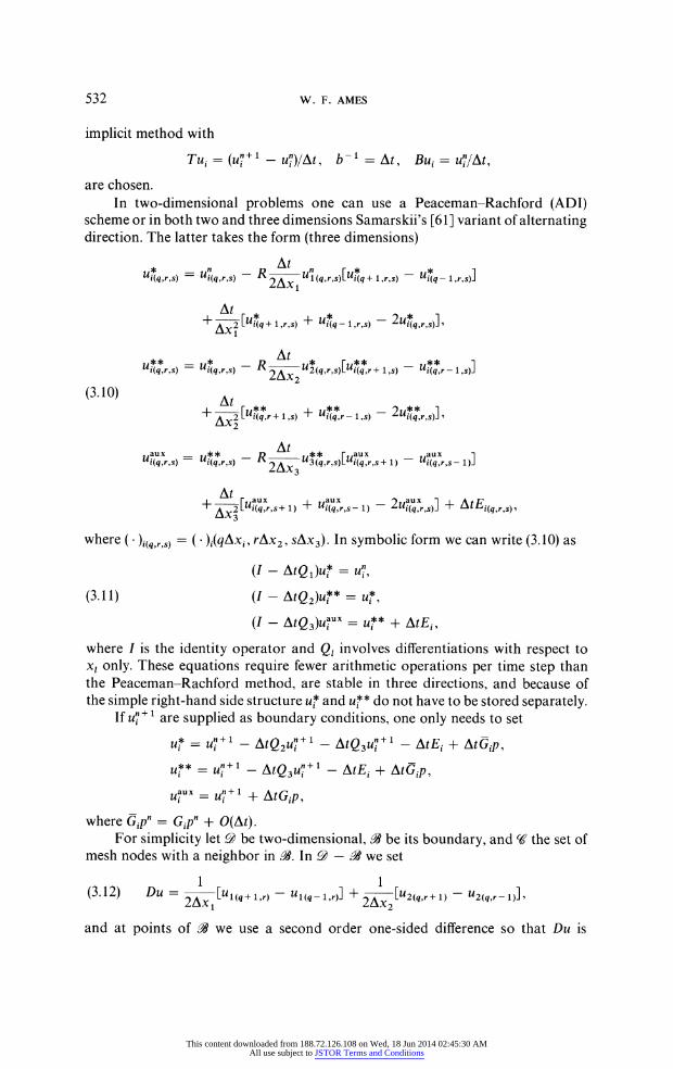
implicit method with

Tui = (u7+' -u')/At, b' = At, Bui = uO/At,

are chosen. In two-dimensional problems one can use a Peaceman-Rachford (ADI)

scheme or in both two and three dimensions Samarskii's [61 ] variant of alternating direction. The latter takes the form (three dimensions)

At At Ui*(q,rs) =Ui(q,r,s) -R2A uj(q,r,j)ui*(q+l,r,s) -Ui*(q- 1,r,s)]

+ At[u* i(q,r,s)]' Ax2 i(q + 1,r,s) + Ui(q - 1,r,s) - 2u*

u'~~ =u~ At Ui(q,r,s) = i(q,r,s)_ R2Ax 2(q,r,js)ui(q,r+ 1,s) - U(q,r i,s)]

(3.10) At + AX2 [U(q,r + 1,s) + U(q,r - ,s) - i(q,rs)

aux ~~~Atauax Ui(q,r,s)U - R 3q,, [ 1 U-i(q,r,s1) ia(uqr s) i(qr s) 2 3(q rs)[Ui(q,r,s+ 1) aux 1)]

+ 2[U(q1r + Uji(q,ir)s - 1)-2Ui(qlr s)] + AtEi(q,r,s),

where ()i(q,r,s) = (*)i(qAxi, rAx2, sAX3)- In symbolic form we can write (3.10) as

(I - AtQ)u = Un

(3.11) (I - AtQ2)u** =u

(I - AtQ3)u4ux = u* + AtEi, where I is the identity operator and Q, involves differentiations with respect to xl only. These equations require fewer arithmetic operations per time step than the Peaceman-Rachford method, are stable in three directions, and because of the simple right-hand side structure u0 and u* do not have to be stored separately.

If u7 + 1 are supplied as boundary conditions, one only needs to set

= Un+1 AtQ2Uin + - AtQ3U7 + - AtEi + AtGip,

u* = Un+_ AtQ3Un+ - AtEi + AtGip,

u IUx = uni + + AtGip,

where Gipn = Gipn + O(At). For simplicity let 9 be two-dimensional, X be its boundary, and W the set of

mesh nodes with a neighbor in X. In 9 - M we set

1 1 (3.12) Du = 2x[Ul(q+l,r)

- U1(q-,r)] + 2Ax[U2(q,r+l)

- U2(q,r-1)]b 2Axi 2AX2

and at points of Mi we use a second order one-sided difference so that Du is




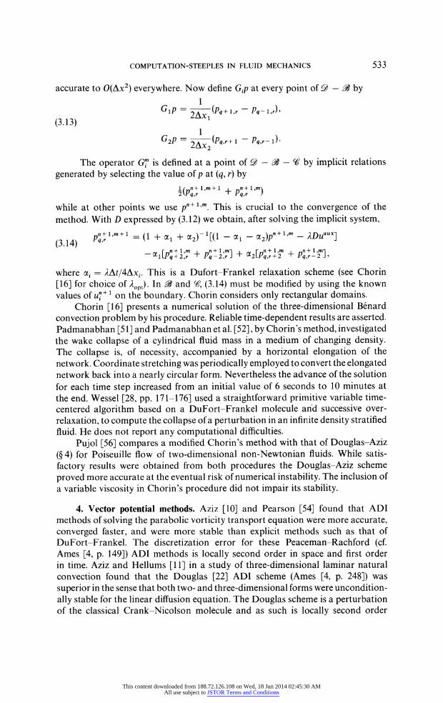
accurate to O(Ax2) everywhere. Now define Gip at every point of 9 - 4 by 1

(3.13) Glp = 2 - (Pq+1,r- Pq-1,r)

G2P = 2AX (Pq,r + 1 - Pq,r - i)

The operator G7 is defined at a point of 9 - - W by implicit relations generated by selecting the value of p at (q, r) by

1 (pn+ l,m+l1 + pn+ l,m) 2(Pq, r + qp,r

while at other points we use pn+l+,m This is crucial to the convergence of the method. With D expressed by (3.12) we obtain, after solving the implicit system,

(3.14) Pq',rm+1 = (1 + al + C2)-1[(1 - - 2)P -DuaUX]

+Id m; + pnl~]+ 2[pnl~jf + I' p+ 1n,m a 1 P4+ 2,r q P- 2,mr] + L-2[Pq,r+ 2 + Pq,r-2]

where ci = .At/4Axj. This is a Dufort-Frankel relaxation scheme (see Chorin [16] for choice of XOp). In X and X, (3.14) must be modified by using the known values of un + 1 on the boundary. Chorin considers only rectangular domains.

Chorin [16] presents a numerical solution of the three-dimensional Benard convection problem by his procedure. Reliable time-dependent results are asserted. Padmanabhan [51] and Padmanabhan et al. [52], by Chorin's method, investigated the wake collapse of a cylindrical fluid mass in a medium of changing density. The collapse is, of necessity, accompanied by a horizontal elongation of the network. Coordinate stretching was periodically employed to convert the elongated network back into a nearly circular form. Nevertheless the advance of the solution for each time step increased from an initial value of 6 seconds to 10 minutes at the end. Wessel [28, pp. 171-176] used a straightforward primitive variable time- centered algorithm based on a DuFort-Frankel molecule and successive overrelaxation, to compute the collapse of a perturbation in an infinite density stratified fluid. He does not report any computational difficulties.

Pujol [56] compares a modified Chorin's method with that of Douglas-Aziz (? 4) for Poiseuille flow of two-dimensional non-Newtonian fluids. While satis- factory results were obtained from both procedures the Douglas-Aziz scheme proved more accurate at the eventual risk of numerical instability. The inclusion of a variable viscosity in Chorin's procedure did not impair its stability.

4. Vector potential methods. Aziz [10] and Pearson [54] found that ADI methods of solving the parabolic vorticity transport equation were more accurate, converged faster, and were more stable than explicit methods such as that of DuFort-Frankel. The discretization error for these Peaceman-Rachford (cf. Ames [4, p. 149]) ADI methods is locally second order in space and first order in time. Aziz and Hellums [11] in a study of three-dimensional laminar natural convection found that the Douglas [22] ADI scheme (Ames [4, p. 248]) was superior in the sense that both two- and three-dimensional forms were unconditionally stable for the linear diffusion equation. The Douglas scheme is a perturbation of the classical Crank-Nicolson molecule and as such is locally second order



534 W. F. AMES

in space and time. While this procedure can and has been used in two-dimensional computation (cf., e.g. Aziz and Hellums [11] in convection and Pujol [56] in non-Newtonian problems) its major impact is felt in three-dimensional problems when the basic equations are recast in vector potentialform.

The vector potential method of Aziz and Hellums [11 ] consists of a transformation of the complete Navier-Stokes equations in terms of a vorticity and a vector potential. These are discretized and solved using the Douglas [22] ADI method for the parabolic portion of the problem and SOR for the elliptic portion. The formulation of the equations of change in terms of the vector potential was found to be an essential ingredient in this analysis. The existence of the vector potential has been known for many years. We shall briefly review the basic concepts herein.

A useful classification of vector fields5 E is possible in terms of the divergence (div) and curl operators. If div E = 0 at every point of a region R the field is said to be solenoidal in that region.6 Physically this means there are no sources or sinks in R. If, at every point of R, curl E = 0 the field is said to be irrotational in R. The classification of fields is as follows:

Class I. Solenoidal and irrotational:

curl E = 0, divE =0.

Class II. Irrotational but not solenoidal:

curl E = 0, divE O.

Class III. Solenoidal but not irrotational:

curl E # O, divE =0.

Class IV. Neither solenoidal nor irrotational:

curlE # O, divE # O.

The velocity field of an incompressible fluid falls into Class III while that of a compressible fluid is of Class IV.

A necessary and sufficient condition for the existence of a scalar potential 0 is that curl E = 0, whereupon 0 is defined by

E = -grad 0 and div E = -div grad =-V0.

Thus, in fields of Class I and II it is always possible to introduce a scalar potential 0, defined by V20 = K (Poisson's equation for a field of Class II).

For fields which are not irrotational (curl E # 0) in some cases it is still possible to employ a scalar function and thus avoid the difficulties usually associated with the more difficult case, that of the vector potential. Suppose that curl E # 0 but there exists a scalar function p such that curl (pE) = 0. In this case a scalar quasi-potential F exists, defined by the equation

(4.1) E= -p-1gradF.

5 In this section a vector is denoted by boldface, viz. E. 6 Much of the foundation research has been with respect to electric and electromagnetic fields,

especially to the Maxwell equations. Thus the terms are reminiscent of that area.




Since 0 = curl (pE) = p curl E + grad p x E it follows that

0 = E curl (pE) = E- p curl E + E - grad p x E

= p(E- curl E) + grad p - E x E.

Consequently, a necessary and sufficient condition for the existence of a quasi- potential is that E . curl E = 0.

From (4.1),

K = div E = -div (p- 1 grad F)

= -p- 1V2F - (grad p )grad F,

where K is zero for Class III and a function for Class IV. Thus a quasi-potential can be determined by solving

(4.2) V2F + p(gradp') grad F =-pK.

The latter equation occurs in field problems associated with inhomogeneous media.

Most solenoidal fields do not admit a potential or quasi-potential but it is always possible to introduce a vector potential A, which, though not as simple as a scalar potential, nevertheless behaves in a somewhat similar fashion. If curl E = B, div E = 0 the vector potential is defined by the relation

(4.3) E = curl A.

Then

(4.4) curl E = curl curl A = grad div A - A = B,

where * is used to denote the vector Laplacian7

(4.5) *A = grad div A - curl curl A.

We can assign any desired value to the divergence of our new vector A. If we take div A = 0 then (4.5) becomes

(4.6) VA B

which is the vector form of Poisson's equation. In Cartesian coordinates (x, y, z) it splits into three scalar Poisson equations,

(4.7) *xA = -Bx, -YA = -By -zA = -Bz.

In the case of a general orthogonal coordinate system (xl, x2, x3) the vector Laplacian is given in Moon and Spencer [43], [44]. To solve a problem using the vector potential we first obtain A from (4.6) and then find E from (4.3).

For completeness we now present the scheme used by Helmholtz in his classic study of vortex motion. In Class IV suppose E has known divergence and curl, neither of which is zero. If U is irrotational (curl U = 0) and V is solenoidal

7 The vector Laplacian is often written V2 but this is an ambiguous notation. Except in the special case of rectangular coordinates, where each component is similar to a scalar Laplacian, the two operators are quite distinct.



536 W. F. AMES

(div V = 0), we suppose

(4.8) E = U + V.

Since curl U = 0, a scalar potential + can be introduced so that

(4.9) U =-grad .

Likewise, since div V = 0 there exists a vector potential A such that

(4.10) V = curl A, divA = 0.

From (4.8) we find

divE = divU + divV = -divgrad =-V2

and

curl E = curl U + curl V = curl curl A =-*A.

Consequently fields of Class IV are evaluated by the solution of the scalar Poisson equation

(4.11) V20= -divE,

and the vector Poisson equation

(4.12) *A = -curl E,

for the scalar potential 0 and vector potential A. Using these we calculate U and V by means of (4.9) and (4.10). Finally E is calculated by means of (4.8). With this introduction we are now in position to discuss the method of the vector potential (Aziz and Hellums [11], Douglass [22]).

The dimensionless equations describing the behavior of fluid layers heated from below are

(4.13) div V = 0,

(4.14) aV//t + V div V = -div P - Gr T + *V,

(4.15) aT/It + V grad T + w = (Pr)f 1V2 T,

where T and P denote deviations in the dimensionless variables from an initial condition of steady conduction, Gr denotes a vector with zero components in the x and y directions and with the Grashof number as its z component and Pr is the Prandtl number. The boundary and initial conditions for the problem of convection in a cube of specified temperature on the upper and lower walls and with insulated side walls are

u = v = w = 0 on all solid boundaries,

(4.16) T(x, y, z, 0) = T (temperature disturbance), T = 0 at z = 0,1, aT/ax = 0 at x = 0,1,

aT/ay = 0 at y = 0, 1.




By elimination of the pressure from the vector equations, (4.14) results in the vorticity transport equation

-Gr T,

(4.17) aW/at + V divW-W -divV = Gr T + VW,

where W = curl V is the vorticity vector. To calculate the velocity from the vorticity, it is convenient to introduce a vector potential j as previously described. This may be viewed as the three-dimensional counterpart of the two-dimensional stream function. It is defined by

V = curl j

and the degree of freedom in its selection permits the vector potential to be solenoidal, i.e., div j = 0. Thus we have

(4.18) = -W.

The set of equations (4.15), (4.17), (4.18) and W = curl V were found to be a convenient form for numerical computation.

A word about the boundary conditions must be inserted here because of a minor controversy between Timman and Moreau which is discussed by Hirasaki and Hellums [36]. Moreau [45] and Hirasaki and Hellums [36] agree that on solid surfaces the proper boundary condition on the normal component of velocity is satisfied if the normal derivative of the normal component of the vector potential vanishes, and if the components of the vector potential tangential to the surface vanish.8 The boundary conditions on the vector potenitial become

(Vhl)x= 2 = 3 =0 atx=0,1,

(4.19) ol = (OV2)y= = (V3 =0 aty=0,1,

1l = 02 = (03). = 0 at z = 0, 1, and those on the vorticity are

=1 = ?, 42 = -OWavX, /3 =VIaX atx = 0,1,

(4.20) 1 = aw/ay, 2 = 0, 43 =-au/ay aty = 0,1,

1 = -av/aZ, 42 = au/aZ, 3 = 0 at z = 0,1.

Here we have written WT = 141, 42, 431 to denote the vorticity vector. In the numerical computation we shall use the following notation:

Q, = Q,(i,j, k) = Q(iAx,jAy, kAz, nAt) = Q(Xi yj, Zk, tn),

VxQn = [Qn(i + , j, k) - Q(i - 1, j, k)]/(2Ax),

xQn = [Qn(i + 1,j, k) - 2Qn(i,j,k) Q(i- 1,j,k)]/(Ax)2,

8 Difficulty in treatment of the boundary conditions is very often reported. Indeed stability problems are often a result of these difficulties.



538 W. F. AMES

=xQn = (Vx - uVx)Qn

yQn= (Vy - VVy)Qn

6zQn = (V2 - wVz)Qn

Corresponding operators Vy, Vz etc. are defined in a similar manner. Any one of the scalar parabolic equations, (4.15) or (4.17), may be written as

(4.21) St = (Sxx - uSX) + (Syy - vSy) + (SZZ - wSz) -, where S represents any of the dependent variables T, 1, 2 and 43. The expression q includes all of the remaining terms, e.g. 0 = w in (4.15). The ADI method of Douglas [22], previously discussed, will now be described for (4.21).

Let us denote by Q the approximate value for S obtained by the finite difference procedure. From the known solution at tn we find a first estimate of the solution Qn*+ 1,at time tn+1 b9

(4.22) 2?x(Qn+1 + Qn) + 6yQn + 6zQn = (Qn+1 - QJ)/At + ?) where 4 is evaluated at n, n + 2 or n + 1 depending upon the method being used. This is followed by

(4.23) 26x(Qn+1 + Qn) + 2{y(Qn+1 + Qn) + 6zQn = (Qn+1 - QJ)/At + 1 and this by

2bx(Qn+l +? Qn) ? 2y(Qn*c*l ? Qn)+ 2?Pz(Qn+l + Qn) = (Qn+l - QJ)/At + ,

(4.24)

where Qn + is the accepted value. Equations (4.22), (4.23) and (4.24) may be simplified by subtracting (4.22) from (4.23) and (4.23) from (4.24), respectively. After some rearrangement the new system becomes

(4.25) [6 - 2(At)']Qn+l = -[6x + 26b + 23z + 2(At) 1Qn + 20, (4.26) [6 - 2(At)']Q*+* = - 2(At) Q* (4.27) [z - 2(At)']Qn+l =6zQn

With u, v, w and 0 known in advance (4.25), (4.26) and (4.27) require the solution of a tridiagonal system of linear algebraic equations three times to find Qn + .

If u, v, w and 0 are not evaluated at the old time step it becomes necessary to perform several iterations at each time step.

The elliptic equations are all of the type

V2S = _0

where k is again a scalar function. The resulting finite difference simulation may be solved by a direct application of the three-dimensional Douglas ADI scheme or by the SOR method of Young (see Ames [4]).

9 One asterisk denotes the first approximation with more asterisks for successive estimates. For the development of the method see Douglas [22] or Ames [4, p. 248]. This ADI scheme reduces to the one proposed by Douglas if we replace our operators b., b and b, by V2, V2 and V2. The nonlinearities in the procedure of Douglas appear only through the term / where / = +(x, y, z, t, S).




Lastly we remark on the four procedures tried in treating the velocity component coefficients of the nonlinear convective terms and the 4 term of (4.21). These were:

(a) Advance values of the dependent variables to the n + 2 level in time. From this calculate the velocity components u, v, and w and the 4 term at n+ 2 and use these to advance the values a full time step. This is essentially the "predictor-corrector" method of Douglas and Jones [24] found so useful by Miller [42] in obtaining numerical solutions of the Burgers' equation u, + uu, = vu., (see ? 5.1).

(b) Evaluate the velocity components u, v, w and 4 entirely at the new level. This requires an iteration.

(c) Evaluate the velocity components u, v, w and 4 at the nth level. No iteration is required if the boundary vorticity is allowed to lag one step behind the inner vorticity. Stability difficulties can arise from this procedure.

(d) Use the average of the new and old values for determining u, v, w and 4 in the nonlinear terms.

In trials (d) was found most suitable from the point of view of stability. In two-dimensional problems both (b) and (d) gave identical solutions but (b) was preferred for storage reasons in three-dimensional problems.

5. New directions. In this section we describe some of the directions that research in numerical analysis is taking. The first of these is the extension of predictor-corrector methods to nonlinear problems by Douglas and Jones. The second, promoted by Bellman and Protter and schools, we shall call "exact" methods. The third, that of finite elements, originally developed for structural mechanics, has been applied to field problems of many types. Thefourth direction involves a reformulation of the problem, usually in terms of new dependent and independent variables. Flugge-Lotz et al. have had much success with such an approach in boundary layer calculations.

We have selected these areas for their future potential with the full realization that research and development in numerical analysis is one of the fastest growing areas of mathematical research. Many of the budding methods are marrying an approximate solution in one or more directions with a numerical scheme. In fluid mechanics one of the earliest computations, by Whitaker and Wendel ([70], also Ames [3, p. 401]), was of this type. Galerkin-type approximations and the associated computations for parabolic equations have been reported by Douglas and DuPont [23]. The tremendous variety and modifications for individual problems is observable in Giese's [31] computer bibliography of numerical solutions of partial differential equations. The continual updating and a computer search routine provides improved accessibility to this file. Excellent summaries of computational methods in various fields of physics are published in the serial "Methods in Computational Physics" edited by Alder et al. [1].

Extensive generalizations of the basic ADI methods have been made with considerable activity by the Russian school. Yanenko's 1967 work, now translated [72], summarizes these generalizations in the so-called method offractional steps which subsumes the majority of the procedures.



540 W. F. AMES

5.1. Predictor-corrector methods. Predictor-corrector methods have been successfully used by many in the numerical solution of ordinary differential equations.

Douglas and Jones [24] have considered

(5.1) uxx = (x,t,u,uxut), O < x < 1, 0 < t < T,

with u(x, 0), u(O, t) and u(1, t) as specified boundary conditions. If either

(5.2) (X, t, u) au

+f2(X, t, U)au + f3(X, t, u) at ax or

I u\ au / u\ (5.3) g =1 x, t, u, / g2 X,t,U, a 'ax' at e

a predictor-corrector modification of the Crank-Nicolson procedure is possible so that the resulting algebraic problem is linear. This is significant since the class given by (5.2) includes the Burgers' equation

uXx = uux + ut

of turbulence and suggests extension to higher order systems in fluid mechanics. The class given by (5.3) includes the equation

a K(u)\au = at(u) au axV exuax at

of nonlinear diffusion. If / is of the form (5.2) the following predictor-corrector analogue combined

with the boundary data ui O, u0,j and UM,j leads to linear algebraic equations. The predictor is'0

(5.4) -= V{ih, ( k, Ui,jj ih5xUij, i(Ui,j+ /2 - Ui,j)}

for i = 1, 2, , M - 1. This is followed by the corrector

2132[Ui,j+1 + Ui,j] = {ih, (j ? 2)k, UiJ+j/24h/IX(U1J+l ? I

k

(5.5) 1 -(Ui,j+ - Ui,j)} k

Equation (5.4) is a backward difference equation utilizing the intermediate time points (j + ')At. Since (5.2) only involves au/at linearly the calculation into the (j + 4) time row is a linear algebraic problem. To move up to the (j + 1)st time we use (5.5) and by virtue of the linearity of (5.2), in au/ax, this problem is also

10 In this section we use the conventional definitions for 6' and p, i.e.,

x j+= +i,j+ I + - I,j+ I 1, PxUi,j = 2[Ui+ 1/2,j + Ui- 1/2,j]-




a linear algebraic problem. As an alternative to (5.4) one may use the predictor

I 6[Ui,Jl2fFh (. 1\2 12_6 ij+1/2 + Ui,j] ih + k, Ui,j, j wxuiX j -(ui,j+ 1/2 -Uii)]

(5.6)

When / is given by (5.3) and we replace the corrector by

1_22[Ui,j+ I + Ui j]

(5.7)

= [ih, j + 4k, Uij + 1/2, 2 6XUi,j+ 1-2 (U + - ui,j)j

then the predictor-corrector system (5.4) and (5.7) generates linear algebraic equations for the calculation of the finite difference approximation.

Douglas and Jones [24] have demonstrated that the predictor-corrector scheme defined by (5.4) and (5.5) converges to the solution of (5.1) when / is specified by (5.2). The truncation error is O[h2 + k2]. When 0 is given by (5.3) convergence was also established when the corrector adopted is (5.7). In this case the error is O[h2 + k3/2].

Miller [42] has investigated and compared this predictor-corrector method with the explicit method and the exact solution (Cole [19]) for a problem given by the Burgers' equation

Ut + uux = vux, 0 < x < 1, 0 < t < T, (5.8) u(0, t) = u(1, t) = 0,

u(x, 0) = sin 7x.

5.2. "Exact" methods. Promoted by Bellman et al. [12], [13], [14] and Noh and Protter [46] and Protter [55] these procedures are based upon two themes. The first is that of using a more efficient way (than that of finite differences) of recreating a function than by storing its values at grid points. The second is that an approximating algorithm should as clearly as possible exhibit the properties of the actual solution. If the solution is nonnegative, this fact should be evident from the relations used to obtain it computationally. Whether or not algorithms of the desired type always exist is an unsolved problem.

Bellman et al. [12], [13], [14] initiated their investigation with the equation

(5.9) ut = UX u(x,0) = g(x)

which has the merit of possessing an implicit general solution

(5.10) u = g(x + ut).

In place of the usual finite difference approximation for the Burgers' equation

(5.11) ut + uux = vuxxn e [,0) = g(x), 0 < x < 1, t > O,

an alternative is adopteci by Bellman et al. [12]. Suppose g(x + 7r) = g(x) and let



542 w. F. AMES

the approximating algorithm be

(5.12) u(x, t + A) = u[x -au(x, t)A, t]

+ (1 2) [U(X ? bA12, t)] + u(x-bW12, -]

where A is the (time) integration step size, and i, a and b are constants which will be determined so that (5.12) is consistent with (5.11) to O(A2). To evaluate i, a and b we expand both sides of (5.12) in a Taylor series to the term in A2, obtaining the equation

(5.13) Ut =-auux (1- - 1 XJ-UX 2

For (5.13) to approximate (5.11) to O(A2) we must have

a = 1/), b = [2v/(1 -)]1/2.

If v is fixed, a and b are functions of i and (5.12) becomes

u(x, t + A) = u[x -u(x, t)(A/)), t]

(5.14) ?1 - i {L-?l(2vA 1/2 ] ? (2vA)1/2t1} + 2~ u _x+ 1- ,t + u _x t- itJ

Let t = 0, A, 2A, , and at each stage of the calculation store u(x, t) by means of the finite sum

M

u(x, t) = E u(t) sin n7rx, n= 1

where the coefficients un(t) are obtained by

un(t) = 2 u(x, t) sin nicx dx

2 R-1 n7tk - Ek Z u(k/R, t) sin R k = R

Thus the values u(k/R, t), k = 1, 2, . , R - 1, store u(x, t) at time t, and by means of (5.14), u(x, t + A) can be obtained.

Various computational results for changes in M, R, and i are discussed by Bellman et al. [12]. A higher order approximation would take the general form

u(x, t + A) = u[x -au(x, t)A, t] N

+ E ai[u(x + biA"/2, t) + u(x -biA/2, t)].

Noh and Protter [46] and Protter [55] use the term "soft solution" as follows: Any function u which satisfies the relation u =f[x - t/(u)] is a solution of ut + O(u)ux = 0. For an arbitraryf (not necessarily differentiable) the expression u = f [x - t/(u)], when it can be solved for u, is called a soft solution. In transport




with chemical reaction

Ut + uux = U', u(x,0) =f(x)

has a soft solution

u1-n = (1 - n)t + f x { 1 2n +? [U -n + (n --l)t] n-}22-1)

for n + 1, n 7 2. For n = 1, 2 we find

(etf[x - u + uetl, n=1,

u(x, t) = f[x + ln (1 - tu)]

1 + tf[x + ln(1 - tu)], 2.

Soft solutions (Protter [55]) can be obtained for a variety of more complicated problems. The existence of soft solutions is useful for testing computational techniques and in the work of Protter suggests natural numerical schemes.

As an alternative to the Bellman et al. procedure the "exact" difference methods of Noh and Protter [46] are available. To illustrate their process we briefly discuss how to obtain various difference methods from the soft solution

(5.15) u = f(x - ut)

of the equation

(5.16) U1 + uux = 0, U(X,0) =f(x), -ooD < x < oo.

In the upper half-plane select a fixed rectangular grid with mesh sizes Ax and At and let Un(X) = U(x, tn) denote the solution of (5.16) at time tn = nAt. Because of the soft solution (5.15) we have

(5.17) un(X) = f[x - tnU(X, ta)] = f[x - tnUn(X)].

Consequently, at the time tn+1 = (n + 1)At, we have from (5.17),

(5.18) u (X) = f {x - tn U[X - Un '(X)At] - AtU (x)}.

On the other hand, using (5.15) directly, we have

(5.19) u (x) = f [x - t+Un + 1 (x)] = f [x - tnUn (X) - Awn ].

Since (5.18) and (5.19) must coincide, we obtain

(5.20) u n(x) = Un[X - AtUn +(x)]

as the basic functional relation. Suppose we have a difference method which determines a solution of a

difference equation corresponding to (5.16). At the mesh points (kAx, nAt), k = 0, ? 1, ? 2, n = 0, 1, 2, ,we denote that solution by {u }n. If this solution satisfies

(5.21) Uk~' = U (Xk - UkAt)

with Xk = kAx, then {Unk+ } will precisely coincide with the soft solution given



544 W. F. AMES

by (5.20). A difference method which, at the mesh points where it is defined, coincides with the corresponding soft solution is called an exact difference method.

A soft solution is prescribed when the initial function f(x) is prescribed. Suppose u?, k = 0, + 1, + 2, , are given and f is determined by linear interpolation between mesh points on the initial line. Thus for Xk - 1? x Xk,

u0 - 0

(5.22) u0(x) = u(x,0) = f (x) = Uk + (X - Xk) - Ax

Since (5.21) is to be satisfied, we have

= U u[xk - U At]

k -k - ukA(Uk - uk-1),

where the second step follows from (5.22). Solving for ul we have 0

{ 1 ? r(u?- u?) if ul > 0, ? r(uo+ - u?) kf~0

where r = At/Ax. Upon replacing 1 by n + 1 and 0 by n, an exact difference method is obtained.

Each interpolation method gives rise to a corresponding exact difference method. If quadratic interpolation is applied at the nth step, the corresponding exact method for (5.16), at step n + 1, is

1 + 1 rAu% - [(1 + rAu%) - 2ur 2A2Un]"2 Uk -r2 A2un

where Aun = Un+1 - un_ 1, A2un = U+ 1 - 2u ? u 1. Other examples are discussed by Noh and Protter [46] and calculations

detailed for problems in gas dynamics.

5.3. Finite elements. Applications of finite elements in fluid mechanics were inevitable and while limited (1972) are being rapidly developed. Specific computations have been made in the areas of potential flow by Argyris et al. (two and three dimensions) [7], Doctors [21], Argyris [6] and deVries and Norris [20]. Flow in porous media has been studied by finite element computation by Javandel and Witherspoon [37], Taylor and Brown [64], Sandhu and Wilson [62] and Volker [68]. Fluid motion in a container has occupied the attention of Tong and Fung [67], Tong [66] and Luk [41]. Argyris and Scharpf [8], Reddi [57] and Reddi and Chu [58] demonstrate the applicability of finite element computation to lubrication problems.

Studies in compressible flow by finite elements are due to Argyris et al. [7] and Argyris [6] while Skiba [63] examines natural convection in rectangular cavities. One of the earliest studies (1964) by Oden and Somoggi [49] concerned low Reynolds number flows, a topic also investigated by Atkinson et al. [9].




Studies involving fluid mechanics and structural vibration include the vibration of submerged structures by Zienkiewicz et al. [73] and an application to supersonic panel flutter by Olson [50]. In these applications to shell-fluid coupled motions the solid wall displacements are assumed to be small. Other references are provided in Zienkiewicz [73], [74] and Oden [48]. A book on the application of finite elements to fluid mechanics is in preparation by Norrie and deVries (1972) [47].

As a typical example we herein describe a finite element procedure for steady inviscid two-dimensional compressible flow. The governing equations are those of momentum

-ap _p-l_ = uux + vuy

(5.23)

_p- 1ap P V + VVY ey

continuity

(5.24) (pu)x + (pv)Y = 0,

and the constitutive relation

(5.25) p = P(P), where u and v are the velocity components in the x and y directions, p is pressure and p is density. From these we may eliminate the pressure and with a potential function 4(u = -Ox, v = - 4Y) obtain the equation

(5.26) (+x- a 2)Oxx + 24x4yoxy + ( 2 _ a2)OYY = 0,

where

a2 = A + b(02 + ,2).

We shall be concerned with a finite element solution of (5.26) in the interior of a plane region D subject to either 4 is specified or do/dn + Q + oX4 = 0 on the boundary C of D. Here Q and ax are prescribed functions of x and y along C. The boundary curve C is assumed to be sufficiently regular so that the divergence theorem is satisfied. A variational or weighted residual formulation can be employed in the finite element development. We shall adopt the former, after the work of Norrie and deVries [47].

If a, G, H, Q and a are functions only of x and y, then a necessary condition for the functional

(5.27) J7(0) = {{D {l2a2[ex ? + 04] - [M + o2] + a2XY Y

X LHO + QO + - s2]

to be stationary is that there exist 4 such that

(5.28) (+x - a2)4xx + 2Gqxy + (02 - a2f 0



546 W. F. AMES

in the interior of D. A comparison of (5.28) with (5.26) shows that they are of the same general form but a and G are known functions of x and y. If the variation is taken as h(x, y), then

h [1(3nx + ( t3ny)-(oxnx + Oyny) (5.29)La2 ?4n)-(n?kn)

+ ?(oxn + nx) - H - Q - ds = 0.

To satisfy (5.29) the following choices of h are of interest: (a) h = 0 on C but is otherwise arbitrary and nonzero in D. This is the case

where the boundary condition is 0 = g(x, y) on C. (b) h is arbitrary and nonzero on C and in D. This requires

(5.30) 3a (nx + '3 ny) -(xnx + 'yny) + a2(kxny + ynx - H - Q - Lx4 = 0

on C. This is the so-called "natural boundary" condition associated with the functional (5.27).

The variational procedure has an Euler equation resembling (5.26) except for the terms a and G. Further, the natural boundary condition (5.30) differs from d4/dn + Q + Loa = 0 on C, originally specified. Thus it is clear that a direct application of this variational procedure to the functional does not yield a solution to the required boundary value problem. An iterative scheme, described below, will overcome this difficulty.

Beginning with an initial value 0?(x, y), we calculate

(5.31) (a0)2 = A + b[(4'0)2 ? (4'O)2]

and

H? = 3 0)2[(4'O)3n + (0k0)3ny1 Ho 3(aO )2 xn y (5.32)

+ [4'0ny + 4'onx]. (ao0)2

From the geometry the unit outward normal to the boundary curve, n, is known and therefore so are its x and y components, nx and ny. H is chosen via (5.32) so that the remaining condition on C (equation (5.30)) becomes

(5.33) d4o/dn + Q + Lx0o = 0.

Upon substituting 4', (5.31) and (5.32) into the functional (5.27) and minimiz- ing, we obtain a solution surface 4" which is also a solution to the following boundary value problem:

(5.34) [(0X)2 - (ao)21'x + 24'?'?41 + [(01)2 - (ao)2]014 = 0




in D, subject to

do' + Q + x?) = {n [(4)1)3 - ()3] ? ny[(01)3 - (00)3]} dn 3(a)2 nXO) +n

(5.35) 1 + (aO)2{(4)14))(4)lny + 4lnx) - (b00)(4?ny + ? onx)}.

Using the solution surface 41, the same procedure 'as that used for 40 is used to generate a new surface 4)2. More generally the iteration technique is obtained from (5.34) and (5.35) by replacing 0 by n and 1 by n + 1.

We should note that the functional given by (5.27) is not unique. Indeed any functional which upon minimization and iteration satisfies (5.26), together with the appropriate boundary conditions, constitutes a proper functional for this problem.

The finite element procedure will now be applied to the iteration method just developed. We remark again that over the region in which the functional (5.27) is applied thefunctions a2, G, H and Q are assumed to befunctions of x and y only. They do not depend upon the particular ̀)n+ 1 whose solution we seek.

To apply the technique the domain D is discretized into finite elements. A particular triangular element, denoted by e, has nodal points labeled i, j, and m in a counterclockwise manner. Next a shape function is chosen" for 4 as an explicit relation for the element whose form is uniquely determined by the nodal values of 0. Choice of the linear expression

(5.36) 0 = al + a2X + a3Y

has the advantage that the derivatives of 4 are constant whereupon the functions a2, G and H appearing in the iteration are constants over each element.

We now complete the formulation for that boundary value problem in which do/dn + Q + Lx4 = 0 must hold on C. We suppose that there are m nodal points in D and n elements. Then it follows that the functional

(5.37) 17(4) = F[01,02, * O)m]

and the set of nonlinear algebraic equations to be solved in the minimization12 process reduce to

OJ/O4p =0, p=1,2, ,m.

5.4. Reformulation in new variables. In analytic studies of nonlinear equations we do not hesitate to employ a great variety of complicated transformations. Quite the opposite appears to be the case in numerical computation. The boundary layer equations have been intensively studied and transformed. Flugge-Lotz (Ames [3, pp. 349-355], [27]) has, in her numerical studies, demonstrated the importance of other independent variables than the primitive ones. A typical example of such behavior is described by Laganelli et al. [40].

" There is only one nodal value for this field problem. At the node i we shall label the potential value /i. Equation (5.36) is the simplest possible shape function corresponding to approximation of the solution surface by elemental triangular planes.

12 If some of the nodal values are prescribed, then these are omitted in the further discussion and the remaining values are renumbered.



548 W. F. AMES

We suppose that a flat plate of nonporous length 1 is fixed in a steady incompressible laminar stream followed downstream by a porous transpiration region. The boundary layer equations with zero pressure gradient in Cartesian coordinates are

(5.38) uX + vy = 0,

(5.39) uux + vuy = vuYY.

The classical Blasius solution describes the boundary layer growth over the nonporous section. This solution evaluated at 1 provides the "initial" condition, at x = 0, for continuation of the solution into the transpiration region. The boundary and initial conditions for that region are

y =0: u =0, v = v, for x > 0,

y -+oo: u u1 for x > 0,

x = 0: u = Blasius solution.

A stream function , defined through the relations

(5.40) u = ao//y, v = - 00/ax

guarantees that the continuity equation (5.38) is satisfied. Upon introduction of these relations into (5.39) we obtain the third order equation

oyoxy - ot/yy = viyyy.

Such a form is undesirable for several reasons, including our relative lack of information regarding their numerical analysis. Thus a way is sought to maintain the second order nature of the equations. This can be accomplished by application of the von Mises transformation (cf. Ames [3]), whereupon (5.39) becomes

(5.41) Au; V ( u au

With the understanding that u = u(x, i/) we drop the subscripts in (5.41) and treat

(5.42) ux= v(uv,)vl which is second order!

After transformation, (5.42) is subject to the following boundary and initial conditions:

= -vex: u = 0, v = v, x > 0,

(5.43) 00 so:- u u1, x > O, x = 0: u = Blasius solution.

Finally, the dimensionless variables

7 = x/l, Q = '1(; , F = 1 - (u/U1)2




are introduced, whereupon (5.43) becomes

or= (1 -r)1/2 02

subject to the auxiliary data

oo F ~~[-0,

= vc(Ul)'/2 , -f7: F r 1.

F(O, d) = Blasius solution (see Laganelli et al. [40] for data). The integration domain does not have orthogonal boundaries (for vc 0 0), since the second boundary condition is applied along the sloping boundary 4 = -f. Irregular mesh point techniques must be employed near that boundary during numerical computation.

REFERENCES [1] B. ALDER, S. FERNBACH AND M. ROTENBERG, eds., Methods in Computational Physics, Academic

Press, New York. vol. 1. Statistical Physics 1963

2. Quantum Mechanics 1964 3. Fundamental Methods in Hydrodynamics 1964 4. Applications in Hydrodynamics 1965 5. Nuclear Particle Kinematics 1966 6. Nuclear Physics 1966 7. Astrophysics 1967 8. Energy Bands of Solids 1968 9. Plasma Physics 1970

[2] C. V. ALONSO, Time dependent confined rotatingflow of an incompressible viscous fluid, Doctoral thesis, University of Iowa, Iowa City, 1971.

[3] W. F. AMES, Nonlinear Partial Differential Equations in Engineering, vol. I, Academic Press, New York, 1965, Chap. 7.

[4] , Numerical Methods for Partial Differential Equations, Thos. Nelson, London; Barnes and Noble, New York, 1969, Chaps. 4, 5.

[5] , Recent developments in the nonlinear equations of transport processes, Indust. Engrg. Chem. Fund., 8 (1969), pp. 522-536.

[6] J. H. ARGYRIS, The impact of the digital computer on engineering science, Aero. J. Roy. Aero. Soc., 74 (1970), pp. 13-42, pp. 111-127.

[7] J. H. ARGYRIS, G. MARECZEK AND D. W. SCHARPF, Two and three dimensional flow using finite elements, Ibid., 73 (1969), pp. 961-964.

[8] J. H. ARGYRIS AND D. W. SCHARPF, The incompressible lubrication problem, Ibid., 73 (1969), pp. 1044-1046.

[9] B. ATKINSON, M. P. BROCKLEBANK, C. C. M. CARD AND J. M. SMITH, Low Reynolds number developingfloows, Amer. Inst. Chem. Engrg. J., 15 (1969), pp. 548-553.

[10] K. Aziz, A numerical study of cellular convection, Doctoral thesis, Rice University, Houston, Tex., 1965.

[11] K. AZIZ AND J. D. HELLUMS, Numerical solution of the three-dimensional equations of motion for laminar natural convection, Phys. Fluids, 10 (1967), pp. 314-324.

[12] R. E. BELLMAN, S. AZEN AND J. M. RICHARDSON, On new and direct computational approaches to some mathematical models of turbulence, Quart. Appl. Math., 23 (1965), pp. 55-67.

[13] R. E. BELLMAN AND R. KALABA, New methods for the solution of partial differential equations, Nonlinear Partial Differential Equations Methods of Solution, W. F. Ames, ed., Academic Press, New York, 1967, pp. 43-54.

[14] R. E. BELLMAN, R. KALABA AND B. KOTKIN, On a new approach to the computational solution oJ partial differential equations, Proc. Nat. Acad. Sci. U.S.A., 48 (1962), pp. 1325-1327.



550 W. F. AMES

[15] A. J. CHORIN, A numerical method for solving incompressible viscous flow problems, J. Comput- ational Phys., 2 (1967), pp. 12-26.

[16] , Numerical solution of the Navier-Stokes equations, Math. Comp., 22 (1968), pp. 745-762. [17] ' On the convergence of discrete approximations to the Navier-Stokes equations, Rep.

1430-106, Courant Institute, New York University, New York, 1968. [18] , The numerical solution of the Navier-Stokes equation for an incompressible fluid, Bull.

Amer. Math. Soc., 73 (1967), pp. 928-931. [19] J. D. COLE, On a quasi-linear parabolic equation occurring in aerodynamics, Quart. Appl. Math.,

9 (1951), pp. 225-236. [20] G. DEVRIES AND D. H. NORRIE, Application of the finite element technique to potential.flow problems,

Reps. 7, 8, Dept. of Mechanical Engrg., Univ. of Calgary, Calgary, Alberta, Canada, 1969.

[21] L. J. DOCTORS, An application ofthe finite element technique to boundary value problems of potential flow, Internat. J. Numer. Math. Engrg., 2 (1970), pp. 243-252.

[22] J. DOUGLAS, JR., Alternating direction methods for three space variables, Numer. Math., 4 (1962), pp. 41-63.

[23] J. DOUGLAS, JR. AND T. DUPONT, Galerkin methods for parabolic equations, SIAM J. Numer. Anal., 7 (1970), pp. 575-626.

[24] J. DOUGLAS, JR. AND B. F. JONES, On predictor-corrector methods for nonlinear parabolic differential equations, J. Soc. Indust. Appl. Math., 11 (1963), pp. 195-204.

[25] E. C. DuFORT AND S. P. FRANKEL, Stability conditions in the numerical treatment of parabolic differential equations, Math. Tables Aids Comput., 7 (1953), pp. 135-152.

[26] H. W. EMMONS, The numerical solution of the turbulence problem, Proc. First Symposium Applied Mathematics, E. Reissner, W. Prager and J. J. Stoker, eds., Amer. Math. Soc., Providence, R.I., 1949, pp. 67-71.

[27] I. FLUGGE-LOTZ, The computation of compressible boundary-layerflow, Nonlinear Partial Differen- tial Equations Methods of Solution, W. F. Ames, ed., Academic Press, New York, 1967, pp. 109-124.

[28] F. N. FRANKIEL AND K. STEWARTSON, eds., Proceedings IUTAM symposium on high speed computing in fluid dynamics, Phys. Fluids, 12 (1969), December.

[29] J. E. FROMM, A method for computing nonsteady incompressible viscous fluid flows, Rep. 2190, Los Alamos Scientific Laboratory, Los Alamos, N.M., 1963; see also Phys. Fluids, 6 (1963), pp. 975-982.

[30] , The time dependent flow of an incompressible viscous fluid, Methods in Computational Physics, vol. 3, B. Adler, S. Fernbach and M. Rotenberg, eds., Academic Press, New York, 1964, pp. 346-382.

[31] J. H. GIESE, A bibliography for the numerical solution of partial differential equations, BRL Mem. Rep. 2114, Ballistic Research Laboratories, Aberdeen Proving Ground, Md., 1971 (supple- ments and computer based searchable file available).

[32] A. E. HAMIELEC, T. W. HOFFMAN AND L. L. Ross, Numerical solution of the Navier-Stokes equations forflow past spheres, Amer. Inst. Chem. Engrg. J., 13 (1967), pp. 220-224.

[33] F. H. HARLOW, Stability of difference equations; Selected topics, Rep. 2452, Los Alamos Scientific Laboratory, Los Alamos, N.M., 1960.

[34] F. H. HARLOW AND J. E. FROMM, Dynamics and heat transJer in the von Karman wake of a rectangular cylinder, Phys. Fluids, 7 (1964), pp. 1147-1156.

[35] F. H. HARLOW AND J. E. WELCH, Numerical calculation of time dependent viscous incompressible flow offluid with a free surface, Ibid., 8 (1965), pp. 2182-2189.

[36] G. J. HIRASAKI AND G. D. HELLUMS, A general formulation of the boundary conditions on the vector potential in three-dimensional hydrodynamics, Quart. Appl. Math., 26 (1968), pp. 331-342.

[37] I. JAVANDEL AND P. A. WITHERSPOON, Application of thefinite element method to transient flow in porous media, Soc. Pet. Engrg. J., 8 (1968), pp. 241-252.

[38] H. B. KELLER, On some iterative methods for solving elliptic differential equations, Quart. Appl. Math., 16 (1958), pp. 209-226.

[39] H. B. KELLER AND H. TAKAMI, Numerical studies of steady viscousflow about cylinders, Numerical Solutions of Nonlinear Differential Equations, D. Greenspan, ed., John Wiley, New York, 1966, pp. 115-140.




[40] A. L. LAGANELLI, W. F. AMES AND J. P. HARTNETT, Transpiration cooling in a laminar boundary layer with solid wall upstream effects, Amer. Inst. Aero. Astro. J., 6 (1968), pp. 193-197.

[41] C. H. LUK, Finite element analysis for liquid sloshing problems, SM thesis, Massachusetts Institute of Technology, Cambridge, Mass., 1969.

[42] E. L. MILLER, Predictor-corrector studies of Burgers' model of turbulent flow, Master's thesis, Univ. of Delaware, Newark, 1966.

[43] P. MOON AND D. E. SPENCER, Field Theory for Engineers, Van Nostrand, Princeton, N.J., 1961, pp. 56, 83.

[44] , Field Theory Handbook, Springer-Verlag, Berlin, 1961, pp. 3, 136, 137. [45] J. MOREAU, Une specification de potential-vector en hydrodynamique, Acad. Sci. Paris, 248 (1959),

pp. 3406-3409. [46] W. F. NOH AND M. PROTTER, Difference methods and the equations of hydrodynamics, J. Math.

Mech., 12 (1963), pp. 149-192. [47] D. H. NORRIE AND G. DEVRIES, Finite Elements and Fluid Mechanics, Academic Press, New York,

in preparation.

[48] J. T. ODEN, Finite Elements of Nonlinear Continua, McGraw-Hill, New York, 1972. [49] J. T. ODEN AND D. SOMOGGI, Finite element application in fluid dynamics, J. Mech. Div. ASCE,

95 (1969), pp. 821-826. [50] M. D. OLSON, Some flutter solutions using finite elements, Amer. Inst. Aero. Astro. J., 8 (1970),

pp. 747-752. [51] H. PADMANABHAN, Wake deformation in density-stratifiedfluids, Doctoral thesis, Univ. of Iowa,

Iowa City, 1969. [52] H. PADMANABHAN, W. F. AMES, J. F. KENNEDY AND T. K. HUNG, A numerical investigation of

wake deformation in density stratifiedfluids, J. Engrg. Math., 4 (1970), pp. 229-241. [53] R. B. PAYNE, Calculation of unsteady viscousflow past a circular cylinder, J. Fluid Mech., 4 (1958),

pp. 81-86. [54] C. E. PEARSON, A computational methodfor viscousflow problems, Ibid., 21 (1965), pp. 611-622. [55] M. H. PROTTER, Difference methods and soft solutions, Nonlinear Partial Differential Equations-

Methods of Solution, W. F. Ames, ed., Academic Press, New York, 1967, pp. 161-170. [56] A. PUJOL, Numerical experiments on the stability of Poiseuille flows of non-Newtonian fluids,

Doctoral thesis, Univ. of Iowa, Iowa City, 1971. [57] M. M. REDDI, Finite element solution of the incompressible lubrication problem, Trans. ASME

Series F, 91 (1969), pp. 524-533. [58] M. M. REDDI AND T. Y. CHU, Finite element solution of the steady state compressible lubrication

problem, Ibid., 92 (1970), pp. 495-503. [59] R. D. RICHTMYER AND K. W. MORTON, Difference Methods br Initial Value Problems, 2nd ed.,

Interscience, New York, 1967, Chaps. 12, 13. [60] Y. RIMON AND S. I. CHENG, Numerical solution of a uniform flow over a sphere at intermediate

Reynolds number, Phys. Fluids, 12 (1969), pp. 949-959. [61] A. A. SAMARSKII, An efficient difference method for solving a multidimensional parabolic equation

in an arbitrary region, U.S.S.R. Comput. Math. and Math. Phys., 3 (1963-1964), pp. 894-926. [62] R. S. SANDHU AND E. L. WILSON, Finite element analysis of seepage in elastic media, Proc. Amer.

Soc. Civil Engrg. EM3, 95 (1969), pp. 641-651. [63] E. SKIBA, A finite element solution of general fluid dynamic problems-natural convection in rec-

tangular cavities, MAS thesis, Univ. of Waterloo, Waterloo, Ontario, Canada, 1970. [64] R. L. TAYLOR AND C. B. BROWN, Darcy flow solutions with aJree surface, J. Hyd. Div. Amer. Soc.

Civil Engrg., 93 (1967), pp. 25-33. [65] A. THOM, Flow past a circular cylinder at low speed, Proc. Roy. Soc. Ser. A, 141 (1933), pp.

651-669. [66] P. TONG, Liquid sloshing in a container, Doctoral thesis, California Institute of Technology,

Pasadena, 1966 (also issued as AFOSR 66-0943). [67] P. TONG AND Y. C. FUNG, The effect of wall elasticity on a liquid in a cylindrical container, Rep.

SM64-40, California Institute of Technology, Pasadena, 1965. [68] R. E. VOLKER, Nonlinear flow in porous media by finite elements, J. Hyd. Div. Amer. Soc. Civil

Engrg., 95 (1969), pp. 2093-2114.



552 W. F. AMES

[69] J. E. WELCH, F. H. HARLOW, J. P. SHANNON AND B. J. DALY, The MAC method. A computing technique for solving viscous incompressible transientfluid-flow problems involving free surfaces, Rep. 3425, Los Alamos Scientific Laboratory, Los Alamos, N.M., 1966. (See also Phys. Fluids, 10 (1967), pp. 927-936.)

[70] S. WHITAKER AND M. M. WENDELL, Numerical solution of the equations of motion for flow around objects in channels at low Reynolds numbers, Appl. Sci. Res. Sec. A, 12 (1963), pp. 91-104.

[71] J. 0. WILKES, The finite difference computation of natural convection in an enclosed rectangular cavity, Doctoral thesis, Univ. of Michigan, Ann Arbor, 1963.

[72] N. N. YANENKO, The Method of Fractional Steps, Springer-Verlag, New York-Berlin, 1971. [73] 0. C. ZIENKIEWIcz, The Finite Element Method in Engineering Science, McGraw-Hill, London,

1971, Chap. 15. [74] , The finite element method: From intuition to generality, Appl. Mech. Rev., 23 (1970),

pp. 249-256.



part 2: anniversary supplement || some computation-steeples in fluid mechanics

Documents