Parents and Children: Education Across Generations in India∗

Pushkar Maitra†and Anurag Sharma‡

November 2009

Abstract

It has been argued that one of the reasons for the uneven distributional effects ofthe high rates of economic growth in India has been the lack of mobility of the Indianpopulation. In this paper we use a nationally representative data set from India to examineone aspect of mobility: that of educational attainment across generations. Specifically,we examine role of parental education on two aspects of child’s educational attainmenti) years of schooling attained and ii) progression across different schooling levels. Wefind that there has been a significant increase in educational attainment of individualsover the last 70 years, with women gaining the most in terms of increases in educationalattainment. Restricting the analysis to adults (those more than 20 years old at the timeof the survey), we find that when we account for the potential endogeneity of parentaleducational attainment, the total effect of parental education on years of schooling oftheir children is not statistically significant indicating an increase in intergenerationaleducational mobility. The analysis of school progression, conducted using a sample of15 − 24 year olds at the time of the survey, reveals that father’s educational attainmenthas a positive and statistically significant effect on the probability of continuing to post-secondary school/college. Private investment (driven primarily by father’s education andhence income) continues to be crucial for young adults to benefit from the opportunitiesoffered by the Indian growth process.

JEL Classification: O12, I21, C31.

Keywords: Intergenerational Transmission of Human Capital, School Progression, Sequen-tial Probit Model, India.

∗Pushkar Maitra would like to acknowledge funding provided by an Australian Research Council DiscoveryGrant. We have benefitted from conversations with Hal Hill, Stephen Howes, Robert Willis and comments byseminar participants at the Australian National University, Canberra and participants at the Indian Economyand Business Update 2009. The usual caveat applies.†Pushkar Maitra, Department of Economics, Monash University, Clayton Campus, VIC 3800, Australia.

Email: Pushkar.Maitra@Buseco.monash.edu.au‡Anurag Sharma, Centre for Health Economics, Monash University, Clayton Campus, VIC 3800, Australia.

Email: Anurag.Sharma@Buseco.monash.edu.au

1

1 Introduction

Mobility is one of the hallmarks of the process of development. In traditional economies

individuals are typically closely attached to the structure they are born into − be it the

occupational structure of their parents or be it the land of their forefathers. In a modern

economy however individuals are able to seek out the best for themselves in terms of their

occupation, location of residence or anything else for that matter.

This is a particularly important issue in the context of India. Among developing countries

India stands out in terms of the remarkably low levels of mobility (see for example Gupta,

2004; Munshi and Rosenzweig, 2009). This lack of mobility means that many sections of the

society are unable to reap the benefits of the phenomenal levels of economic growth that the

country has experienced over the last two decades. Indeed by a number of different measures,

inequality in outcomes has actually increased over the relevant period. Part of this could be

due to the fact that in a society characterized by lack of mobility, the gains from growth accrue

disproportionately across the population and in particular some sections of the population

are unable to take advantage of the opportunities that the growth process in the country has

provided. For the benefits of the growth process to be distributed in a much more egalitarian

manner, the population needs to be mobile, both vertically (in terms of increasing their levels

of educational attainment across generations) and spatially (in terms of physically moving to

the location that provides the best opportunities).

In this paper we re-examine the issue of differences in human capital accumulation over

generations, i.e., examine the issue of vertical (or inter-generational) mobility in educational

attainment. In particular we focus on the issue of the correlation between education levels of

parents and children, which reflects the degree of equality of opportunity in a society (Becker

and Tomes, 1986). There are several mechanisms through which parental education can affect

human capital outcomes of their children. For example, maternal education can improve

efficiency of human capital production leading to increasing returns, across generations, in

parental human capital (Becker et al., 1990). Alternatively, one could consider the education

level of mothers to be a function of their endowed human capital, which is positively correlated

with that of their children (see for example Rosenzweig and Wolpin, 1994; Behrman and

2

Rosenzweig, 2002).

While the issue of intergenerational mobility in educational attainment has received some

attention in other countries (see Behrman et al. (2000); Bourguignon et al. (2003) for a

discussion of this issue in the context of Brazil and Thomas (1996) for a discussion on South

Africa), the issue has received surprisingly little attention in the context of India. To the best

of our knowledge the only paper that explicitly addresses this issue in the context of India

is Jalan and Murgai (2008). They use data from the 1992-93 and 1998-99 National Family

Health Surveys to examine inequalities in educational outcomes across groups of individuals

and the perpetuation of these inequalities across generations. Our paper builds on the work

by Jalan and Murgai (2008). Using a nationally representative data set for India (the Indian

Human Development Survey) collected in 2005 we examine the following questions. First,

how has the profile of educational attainment of adults (defined as at least 20 year old at the

time of the survey) changed over generations? Second, what is the effect of parental education

on the educational attainment of individuals? In this context we explicitly account for the

potential endogeneity of parental educational attainment in any regression that examines

the effect of parental educational attainment on the schooling of the next generation. This

potential endogeneity arises from the fact that parental educational attainment might be

correlated with some of the unobserved determinants of the child’s schooling. Alternatively

the unobserved components of the child’s educational attainment might be correlated with the

unobserved components of that of the parents. Both of this could result in biased estimates.

Finally restricting the sample to young adults (aged 15 − 24 at the time of the survey) we

examine effect of parental educational attainment on the propensity to continue in school for

these individuals. These individuals form an important demographic because they are the

ones who need to be able to take advantage of the opportunities that are likely to come their

way as a result of the growth process.

In addition to the issue of mobility (and its implications for the process of development)

the issue of children’s human capital accumulation is particularly crucial for India where

proportion of school going children (aged between 0−14 years) is projected to be 23% of total

population by 2025 (compared to 18% in China and the US and 13% in Europe UN, 1999).

Overall however, as Kingdon (2007) argues, the story of India’s educational achievements is

one of mixed success. On the one hand while India has 22% per cent of the worlds population,

3

it has 46% of the worlds illiterates, and is home to a high proportion of the worlds out-of-

school children and youth. On the other hand, it has made significant progress in raising

schooling participation. Additionally it has emerged as an important player in the worldwide

information technology revolution on the back of large numbers of well-educated computer-

science and other graduates. However as Kingdon (2007) also argues, the base of the Indian

education pyramid is weak and this has serious implications for the extent of overall human

capital accumulation in the country.

Given the linkage between human capital accumulation and economic growth (Barro, 2001),

an analysis of inter-generational mobility in educational attainment and also of the determi-

nants of school progression could help predict the major trends in future economic growth

in India. The results from such an analysis can help in the design of an effective policy to

augment the human capital of children. There is broad consensus in the literature on the

positive effects of parental education on school enrolment for both developed and developing

countries. The empirical analysis in this paper goes a step further and examines the effect of

parental education on the “progression” of children across different enrolment levels.

Why is school progression important? In recent years the issue of school dropouts (the inverse

of school progression) has been of increasing concern to policy makers both in developed and

developing countries. While there might be “valid” economic reasons for dropping out of

school early, the consequences of such action can be quite severe. In developing countries

children typically drop out of school because the current income requirements of the household

exceed the expected returns from continuing to remain in school. Obviously this has significant

long-term impacts − low educational attainment and consequently low levels of human capital

accumulation, which in turn imply that future income earning opportunities are limited and

lifetime incomes are low. Additionally there is an inter-generational effect: children born to

parents with low levels of education are themselves more likely to end up with low levels of

educational attainment.1

1However this is not only a developing country problem. Even in developed countries early school dropoutsand non-completion of schooling is fast becoming a serious problem. For example in Australia (an OECDcountry), studies have shown that almost one third of students drop out from high school each year and mostof them never gain a year 12 or equivalent qualification. High school dropouts are much more likely to beunemployed, or to have given up looking for work, or to have low lifetime incomes. They are more likely to havepoor numeracy and literacy skills, which affect their productivity, social participation and decision-making.While half of the male 15 to 19-year-olds who leave school early end up with full-time work, as do 65% of 20to 24 year olds who dropped out of school, the story is much more depressing for women. Less than 35% of

4

The empirical analysis of school progression uses the correlated sequential probit estimation

technique (see Lillard and Willis, 1994; Pal, 2004) which has several advantages: First, it

allows us to identify the children who have progressed much less than others and also to

locate at what level of schooling this has happened; second, it controls for the self selection

of students into the next higher level of schooling; and third, it allows us to (potentially) use

different control factors for each transition. The results from this analysis therefore enable

us to decompose the effect of parental education at different transitions. For example this

technique enables us to identify the scenario where education of both the parents is significant

for school enrolment but only father’s education matters for progression to higher schooling

level.

2 How has Education Increased over Generations?

This paper uses data from the Indian Human Development Survey 2005 (IHDS). This survey

is a nationally representative, multi-topic survey of 41,554 households in 1,503 villages and

971 urban neighborhoods across India. Two one-hour interviews in each household covered

topics concerning health, education, employment, economic status, marriage, fertility, gender

relations, and social capital. Survey was conducted between November 2004 and October

2005 with a response rate of 92%. For the first part of the paper (sections 2 − 3) we restrict

ourselves to individuals born in 1985 or before (who are at least 20 years old at the time

of the survey). The relevant sample means are presented in columns (1) and (2) in Table

1 (corresponding to Sample 1) for the rural and urban sample respectively. We want to

highlight the difference in the average years of schooling by residence: the average years of

schooling is 4.34 years for rural residents and 7.69 years for urban residents (the difference is

statistically significant at the 1% level).

We start by presenting selected descriptive statistics on the how education has changed over

generations. Figure 1 presents the average years of schooling attained by birth cohort. There

is no doubt that Indians have become more educated. For urban males, the average years of

schooling has increased from close to 6 years for individuals born in 1930 or before (Cohort

women in both age groups who left school early have a full-time job and more than a third of the 20 to 24year olds are unemployed (see Spierings, 1999).

5

1) to 10 years for individuals born between 1981 and 1985 (Cohort 12). The corresponding

increases are from 2 to 9 years for urban females, 2 to 7.5 years for rural males and 1 to 5.5

years for rural females. The decline in the average years of schooling for individuals born after

1985 is essentially due to the fact that a number of individuals belonging to these cohorts are

at school at the time of the survey and have not attained the maximum level of education.

To be more specific, while 3.59% of individuals born in 1985 or before are enrolled in school

at the time of the survey; this percentage rises to 56.73% for individuals born over the period

1986 − 1990 and to 92.13% for individuals born over the period 1991 − 1995.

Mean growth rates in educational attainment are presented in the first row of Panel A in

Table 2. These are the coefficient estimates from a standard OLS regression of the years of

schooling on birth year.2 Separate regressions are conducted for males and females and for

those residing in rural and urban areas (i.e. we present four sets of results). The average

years of education has increased by 1.2 years each decade for urban females and around 1

year each decade for rural males and females. The average years of schooling has increased by

about 0.5 years per decade for urban males, though it is important to note that the average

years of schooling for urban males is quite high to begin with. Figure 2 presents the lowess

plots of the years of schooling on the year of birth. These lowess plots essentially tell the

same story; additionally they highlight the non-linearity in the relationship between the year

of birth and the years of schooling attained, something not explicitly addressed in the OLS

regressions presented in Table 2, Panel A.

Panels B, C, D and E in Table 2 present the marginal effects from probit regressions for the

highest level of education attained. The dependent variables in the regressions are: Enrolled

in school (which takes the value of 1 if the child has any schooling and 0 otherwise), Enrolled

in middle school (= 1 if the years of schooling attained by the individual more than 5 and 0

otherwise), Enrolled in post-secondary school (= 1 if the years of schooling attained by the

individual is more than 10 and 0 otherwise), Enrolled in college (= 1 if the individual has

ever attended college and 0 otherwise). The biggest gainers are the females with rural females

gaining more than urban females. The marginal effects presented in Panel B show that the

probability of enrolling in school increases by nearly 16 percentage points every decade for

rural females; followed by 8.4 percentage points every decade for urban females, 7.6 percentage2The sample is restricted to individuals born in 1985 or earlier.

6

points every decade for rural males and finally 2.6 percentage points every decade for urban

males. Rural females have gained in every stage: the probability of enrolling in middle school

has increased by 10.1 percentage points every decade and the probability of enrolling in post-

secondary school has increased by 7.5 percentage points every decade.

Next we examine the extent of unevenness in the growth of educational attainment across

generations. Table 3 essentially repeats the same analysis as in Panel A of Table 2, but

this time we stratify the sample on the basis of religion (columns 2− 5) and caste (columns

6 − 10). As a point of comparison we present the results for the full sample in column 1:

these are the coefficient estimates presented in Table 2, Panel A.3 There is, not surprisingly, a

great deal of variation across the different religions and castes and unfortunately (particularly

in the case of females) there is very little evidence of catching up by those with the lowest

educational attainment. For example when we look at the sample of rural females, not only is

the mean years of schooling the lowest among the Muslims, so is the growth rate. While the

years of schooling for those belonging to other religions has increased on an average by 1.2

years every decade, that for the Muslims has increased by 0.8 years every decade. Given the

initial difference in average years of schooling (0.27 years for Muslims compared to 0.38 years

for those belonging to other religions for those born before 1930), the difference in growth

rates implies that the average years of schooling attained by rural females belonging to other

religions is more than double that of Muslims in 1980. Looking at the results for the different

castes, it is clear that individuals belonging to scheduled tribes (ST) have fared the worst in

terms of educational attainment.

3 Effect of Parental Education

Educational attainment is typically influenced by both public and private investments in

education. While state policy typically drives the former, parental education is a crucial part

of the latter; indeed parental education is one of the most important determinants of a child’s

education. In a rigid society with no mobility, parental education completely determines the

educational attainment of the child. Put in another way, after controlling for other socio-3Theoretically the concept of caste does not and should not exist for non-Hindus; however partly because

of history and partly because of affirmative action policies aimed at certain castes, many non-Hindus appearto hold on to their caste.

7

economic characteristics that potentially affect educational attainment of an individual, the

greater the influence of paternal and maternal education, the lower is the extent of inter-

generational mobility.

The information on parental educational attainment is available only for a subset of the full

sample. The descriptive statistics are presented in columns (3) and (4) in Table 1 (corre-

sponding to Sample 2) for the rural and urban samples respectively. Most of the averages are

similar to the full sample. The new variables here are the years of schooling attained by the

father and the mother. Fathers are more educated compared to mothers in both rural and

urban households (in both cases the average difference in the years of schooling attained is

around 3 years) and also both fathers and mothers in urban households are more educated

compared to their rural counter parts (again the difference is around 3 years at the mean).

To examine the issue of the association between parental education attainment and child edu-

cational attainment we start by presenting in Figure 3 the lowess plots from a non-parametric

regression of the years of schooling attained by an individual on the years of schooling at-

tained by the father and mother. These plots essentially capture the relationship between the

educational attainment of the father or mother and that of the child using a non-parametric

regression of the form:

Years of schooling of the child = f(Years of schooling of the father or mother) + ε

The results are interesting. First, there is a positive correlation between parental education

and children’s education. Second, on an average, the educational attainment of children is

greater than the educational attainment of the fathers, for fathers with less education; i.e.,

if the father has attained x years of schooling, the child has on an average attained more

than x years of schooling − the lowess plots always lie above the 45◦ line for fathers with

low education. The slope is however generally less than 1, indicating that an additional year

of schooling attained by the father is not associated with an additional year of schooling

attained by the child. For more educated fathers, children have on an average less years of

schooling compared to fathers. It is however worth noting that the lowess plots intersect the

45◦ line at a fairly high level of education attained by the father − to be precise beyond

10 years of schooling. Given that the average years of schooling of rural fathers is 4.1 years

and that of urban fathers is 7.1 years, this implies that for the sample under consideration

8

children are generally more educated than the fathers. Third, while broadly the effects are

similar when we look at the association between the educational attainment of the mother

and that of the child, there is however a very noticeable gender effect in this case. For mothers

with low educational attainment (defined as mothers having less than 3 years in the urban

sample and less than 8 years in the rural sample), on an average, if the mother has attained x

years of schooling, both sons and daughters have attained more than x years of schooling and

the educational attainment of sons exceeds that of daughters. However for more educated

mothers, on an average the educational attainment of daughters exceeds that of the sons.

This result has significant policy implications. Policy makers and economists have argued

of the need to increase educational attainment of mothers as the most important way of

reducing the educational gender gap. While this is true, it is also true that a threshold level

of education (that is not constant by gender and or region of residence) must be attained

before this policy can work.

However in trying to analyze the effect of parental educational attainment on that of the

child, we face a potential endogeneity problem: the years of schooling of the mother and

father are potentially endogenous arising from the fact that parental educational attainment

could be correlated with some of the unobserved determinants of child’s schooling4 and failure

to correct for this endogeneity would result in biased estimates. The problem is to find

proper instruments that are correlated with parental educational attainment and not with

the educational attainment of the child. This is a difficult problem in a non-longitudinal data

set.

There are growing number of studies focussing on determinants of child schooling in developing

countries. Pal (2004) analyzes child schooling data for Peruvian households and reports that

parental education positively affects child schooling at primary and secondary levels, but

not at post-secondary levels. Singh (1992) examines major economic aspects of demand of

schooling of farm operators in Brazilian rural households and finds that parental education

positively affects household demand for children’s education with mothers education having

larger effect than that of the father. A similar result is reported by Maitra (2003) for demand4For example it might result in inter-generational transmission of values that result in the next generation

attaining more schooling. Alternatively the unobserved components of child’s schooling decision might becorrelated with parents unobserved characteristics (one such example is genetic characteristics).

9

for schooling in Bangladesh. Dreze and Kingdon (2001) use data on 1143 households for

rural north India to analyze the impact of school quality on school participation. They find

that probability of participation increases with parental education, though mother’s education

does not have significant effect on male school participation. Evidence from Pakistan suggests

that parental education significantly increases the education of their sons (Holmes, 2003).

Unfortunately few studies have explicitly accounted for potential endogeneity of parental

educational attainment. One notable exception is Lillard and Willis (1994) who explicitly

account for this endogeneity using data from Malaysia.

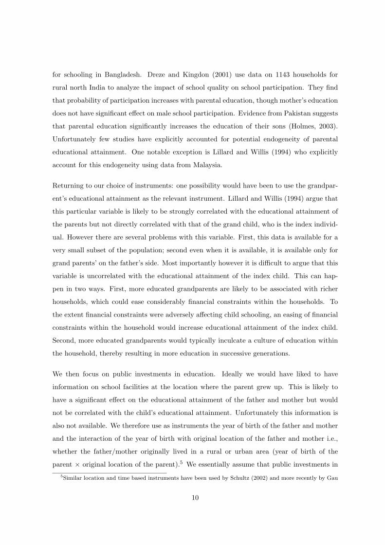
Returning to our choice of instruments: one possibility would have been to use the grandpar-

ent’s educational attainment as the relevant instrument. Lillard and Willis (1994) argue that

this particular variable is likely to be strongly correlated with the educational attainment of

the parents but not directly correlated with that of the grand child, who is the index individ-

ual. However there are several problems with this variable. First, this data is available for a

very small subset of the population; second even when it is available, it is available only for

grand parents’ on the father’s side. Most importantly however it is difficult to argue that this

variable is uncorrelated with the educational attainment of the index child. This can hap-

pen in two ways. First, more educated grandparents are likely to be associated with richer

households, which could ease considerably financial constraints within the households. To

the extent financial constraints were adversely affecting child schooling, an easing of financial

constraints within the household would increase educational attainment of the index child.

Second, more educated grandparents would typically inculcate a culture of education within

the household, thereby resulting in more education in successive generations.

We then focus on public investments in education. Ideally we would have liked to have

information on school facilities at the location where the parent grew up. This is likely to

have a significant effect on the educational attainment of the father and mother but would

not be correlated with the child’s educational attainment. Unfortunately this information is

also not available. We therefore use as instruments the year of birth of the father and mother

and the interaction of the year of birth with original location of the father and mother i.e.,

whether the father/mother originally lived in a rural or urban area (year of birth of the

parent × original location of the parent).5 We essentially assume that public investments in5Similar location and time based instruments have been used by Schultz (2002) and more recently by Gau

10

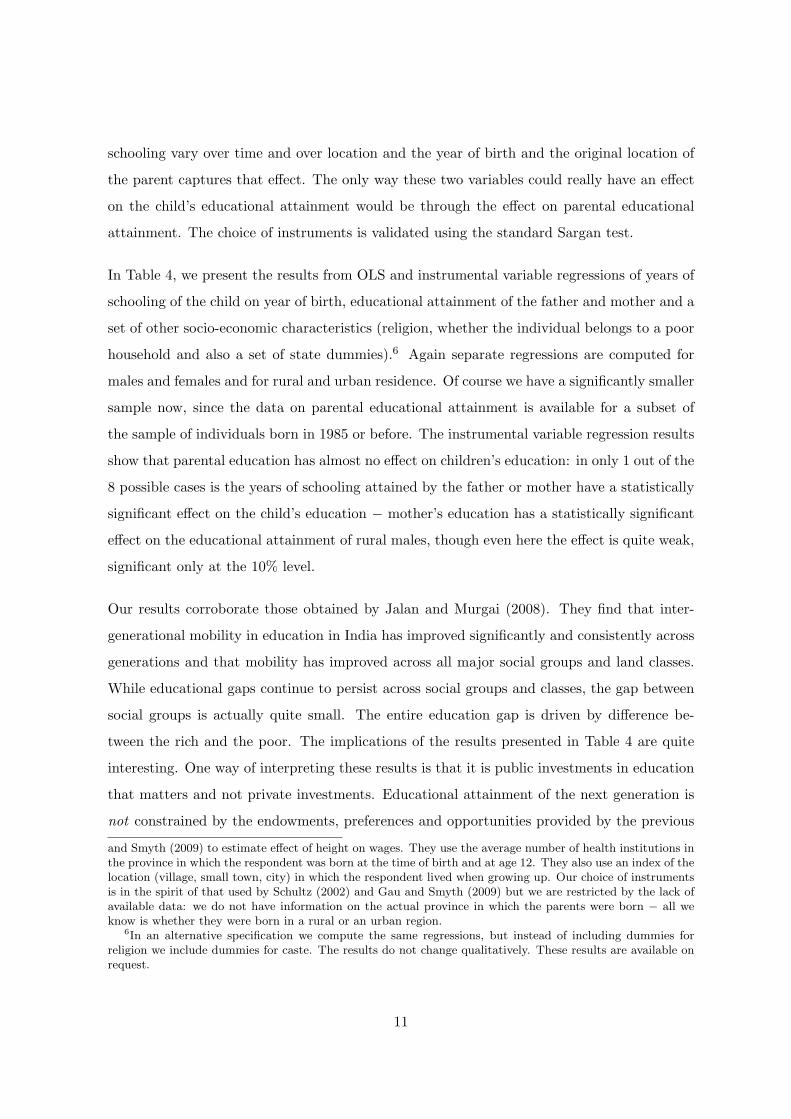
schooling vary over time and over location and the year of birth and the original location of

the parent captures that effect. The only way these two variables could really have an effect

on the child’s educational attainment would be through the effect on parental educational

attainment. The choice of instruments is validated using the standard Sargan test.

In Table 4, we present the results from OLS and instrumental variable regressions of years of

schooling of the child on year of birth, educational attainment of the father and mother and a

set of other socio-economic characteristics (religion, whether the individual belongs to a poor

household and also a set of state dummies).6 Again separate regressions are computed for

males and females and for rural and urban residence. Of course we have a significantly smaller

sample now, since the data on parental educational attainment is available for a subset of

the sample of individuals born in 1985 or before. The instrumental variable regression results

show that parental education has almost no effect on children’s education: in only 1 out of the

8 possible cases is the years of schooling attained by the father or mother have a statistically

significant effect on the child’s education − mother’s education has a statistically significant

effect on the educational attainment of rural males, though even here the effect is quite weak,

significant only at the 10% level.

Our results corroborate those obtained by Jalan and Murgai (2008). They find that inter-

generational mobility in education in India has improved significantly and consistently across

generations and that mobility has improved across all major social groups and land classes.

While educational gaps continue to persist across social groups and classes, the gap between

social groups is actually quite small. The entire education gap is driven by difference be-

tween the rich and the poor. The implications of the results presented in Table 4 are quite

interesting. One way of interpreting these results is that it is public investments in education

that matters and not private investments. Educational attainment of the next generation is

not constrained by the endowments, preferences and opportunities provided by the previous

and Smyth (2009) to estimate effect of height on wages. They use the average number of health institutions inthe province in which the respondent was born at the time of birth and at age 12. They also use an index of thelocation (village, small town, city) in which the respondent lived when growing up. Our choice of instrumentsis in the spirit of that used by Schultz (2002) and Gau and Smyth (2009) but we are restricted by the lack ofavailable data: we do not have information on the actual province in which the parents were born − all weknow is whether they were born in a rural or an urban region.

6In an alternative specification we compute the same regressions, but instead of including dummies forreligion we include dummies for caste. The results do not change qualitatively. These results are available onrequest.

11

generation and that state policy has been successful in severing this link.

There are no surprises in the coefficient estimates of the additional control variables included

in Table 4. Educational attainment of Muslims is significantly lower compared to that of Hin-

dus (the Muslim dummy is always negative and statistically significant); the Christian dummy

is never statistically significant and in the rural areas individuals belonging to other religions

(including Sikhs, Jains and Buddhists) have significantly lower educational attainment com-

pared to Hindus. The Poor household dummy is always negative and statistically significant,

implying that individuals in poor households (at the time of the survey) have fewer years of

schooling. Interpretation of this variable could however be problematic because this variable

tells us whether the household is poor or not at the time of the survey and not (necessarily)

at the time when schooling decisions were made.7

The rest of this paper further examines this link between parental education and child ed-

ucation, but with one difference. We examine the effect of parental education on school

progression rather than school completion. Such an analysis enables to identify factors which

affect school progression and thus drop out rates. We use a restricted sample of individuals

who are 15 − 24 year old at the time of the survey.8 Given the cross-sectional nature of the

data means though that the information on household and socio-economic characteristics is

available only at the time of the survey. It is difficult to interpret the results if we consider

individuals who are far removed from the time when actual education decisions were made.

By focussing on this sub-sample, we are able to also examine the role of other socio-economic

characteristics (including sibling characteristics) on educational attainment.

4 A Sequential Probit Model for Educational Attainment

4.1 Methodology

We examine school progression as a relevant indicator of child schooling in India within a

dynamic sequential framework. In this set up, school progression is conditional on attainment7On the other hand this was not a period of rapid economic growth in India. This also means that mobility

out of poverty might also not have been particularly high.8Traditionally the school going age group is 6 − 18. However in many developing countries children delay

their initial enrolment and also continue to remain in school beyond the age of 18.

12

at the previous level and also self-selection into the next higher level of schooling. This is

based on a correlated sequential probit model (see Lillard and Willis, 1994; Pal, 2004), which

allows us to identify the children who have progressed much less than others and also to

locate at what level of schooling this has happened. This is important for any assessment

of policies geared to boost child schooling because it is based on a full understanding of the

nature of the selection process across different levels of schooling. We will, in particular,

focus on the following three levels of transition: (a) considering all sample children, whether

a child gets enrolled in a primary school (s = 1); (b) among those enrolled in primary

schools, whether a child moves on to the middle/secondary level (s = 2); and (c) among those

enrolled in secondary schools, whether a child moves on to the post-secondary level (s = 3).

Figure 4 presents a schematic representation of this sequential framework. While decision

(a) relates to school enrolment decisions, (b) and (c) relate to school attainment, i.e., school

progression from primary to middle/secondary level and that from the middle/secondary to

post-secondary levels respectively. Our analysis of child school progression therefore combines

both indicators of enrolment and attainment in a sequential framework. Movement from

primary to middle/secondary level is conditional on the successful completion of the final

year of the primary school; similarly moving from middle/secondary to post-secondary level

requires one to “pass” the final year at the secondary level. We take account of the process

of self-selection at each higher level as only a fraction of children successfully completing

primary (or secondary) schools will move on to the secondary (or post-secondary) schools. For

example, decision (b) selects those who successfully complete primary schooling and move on

to middle/secondary school and (c) selects those who successfully complete middle/secondary

school and move on to the post-secondary level. The framework that we use allows the

determinants of selection to vary across the different transitions. In addition to the child’s

ability, we control for sibling composition, household resource constraint, parental preferences

and some community characteristics and obtain selectivity corrected correlated sequential

probit estimates of school progression.

The use of the sequential probit model also allows us to address the important issues of prob-

ability spikes and censoring. Surveys typically measure schooling attained by the years of

education attained (or the highest grade completed). This leads to several problems. First,

even though desired schooling might be a continuous variable, the researcher only observes

13

only discrete years of schooling. Second, data on education attainment from developing

countries is often characterized by a large mass point at zero years of education and similar

probability spikes at primary and secondary school completion levels, where progress to the

next level is often impeded by school fees and entrance requirements. OLS estimation is there-

fore inappropriate under this set up. An alternative would be to use an ordered probit/logit

model of attainment of specific levels of schooling. While this approach takes into account the

discreteness of the data and the probability spikes, it fails to account for the censoring in the

data arising from the fact that some children are enrolled in school at the time of the survey.

One can argue that the desired level of schooling equals the completed years of education for

the children that are not currently enrolled in school. However for children that are currently

enrolled in school, the desired years of schooling exceeds the years of completed schooling.

These observations are therefore right censored. A sequential model, since it is concerned only

with the probability of continuing on to a certain level (conditional on successful completion

of the previous level), is able to avoid the issue of censoring. By definition it addresses the

issue of probability spikes. In addition it accounts for the selection into stages, which ordered

probit/logit models typically do not.

Standard modeling techniques used in most existing studies on child schooling (including those

specific to India) fail to capture the specific characteristics of child schooling in India, where

primary enrolment rates are high along with high failures and drop out rates. Thus school

progression is a better indicator of child schooling than simply school enrolment/attainment

measured by the years of schooling. We determine child school progression in dynamic frame-

work, using sequential probit model, which is argued to be better than the corresponding

ordered probit estimates. For someone at the secondary level, for example, the sequential

probit model takes account of the fact that the person has completed the primary level to

reach the secondary level while the ordered probit model neither takes account of the achieve-

ment at the previous level nor does it correct for any self-selection into the next higher level

of schooling.

We consider four mutually exclusive levels of schooling: none, primary, middle/secondary and

14

post-secondary/college. Define

ω =

0 if years of schooling is 01 if years of schooling is 1− 5 years2 if years of schooling is 6− 10 years3 if years of schooling is 10+ years

(1)

The three levels of transition that we have talked about above follow directly from equation

1. The first decision is whether to attend school at all (s = 1); for those who attend school,

the second decision is whether to continue on to middle/secondary school or stop in primary

school (s = 2); for those who attend middle/secondary school is whether to stop there or

continue to post-secondary school or college (s = 3).

Our primary interest is in modeling the transition from one stage to another. For each

individual i we can write a probit index function at each decision node s as follows:

Isi = βsXsi + δi + usi; s = 1, 2, 3 (2)

Equation 2 is the propensity to continue in school (move from one level to the next higher level)

and includes covariates (Xsi), which vary by individual and (potentially) by decision level.

For example, some variables like parental education, religion are constant across decisions,

but there might be other variables (like number of siblings, state of residence) that vary

across decisions. Since the data set that we use is cross-sectional, we do not include in Xsi

any variable that varies over decisions. Individual variables affect the propensity to attend

school differently depending on the transition stage s, and therefore βs is decision specific. For

example it is feasible that educational attainment of the mother has a positive and statistically

significant effect on the propensity to enrol in school, but not on the conditional probability

of continuing on to middle/secondary school and on to post-secondary school.

We also account for heterogeneity in the propensity to continue in school, assumed to capture

all correlation across schooling decisions. This is represented by the residual term δi, which

is constant across the different schooling decisions. The remaining residual terms at each

decision point (usi) are assumed to be independent of δi and of each other. Both δi and usi

are assumed to be normally distributed as follows: usi ∼ N(0, 1) and δi ∼ N(0, σ2δ ).

Individual i will move from level ω to level ω + 1 if Isi > 0 and drop out otherwise.9 So we9A move from level ω to level ω + 1 is denoted by transition level s.

15

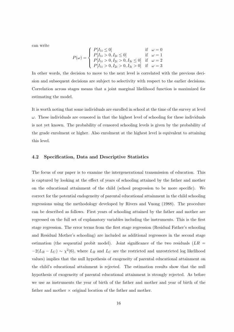
can write

P (ω) =

P [I1i ≤ 0] if ω = 0P [I1i > 0, I2i ≤ 0] if ω = 1P [I1i > 0, I2i > 0, I3i ≤ 0] if ω = 2P [I1i > 0, I2i > 0, I3i > 0] if ω = 3

In other words, the decision to move to the next level is correlated with the previous deci-

sion and subsequent decisions are subject to selectivity with respect to the earlier decisions.

Correlation across stages means that a joint marginal likelihood function is maximized for

estimating the model.

It is worth noting that some individuals are enrolled in school at the time of the survey at level

ω. These individuals are censored in that the highest level of schooling for these individuals

is not yet known. The probability of censored schooling levels is given by the probability of

the grade enrolment or higher. Also enrolment at the highest level is equivalent to attaining

this level.

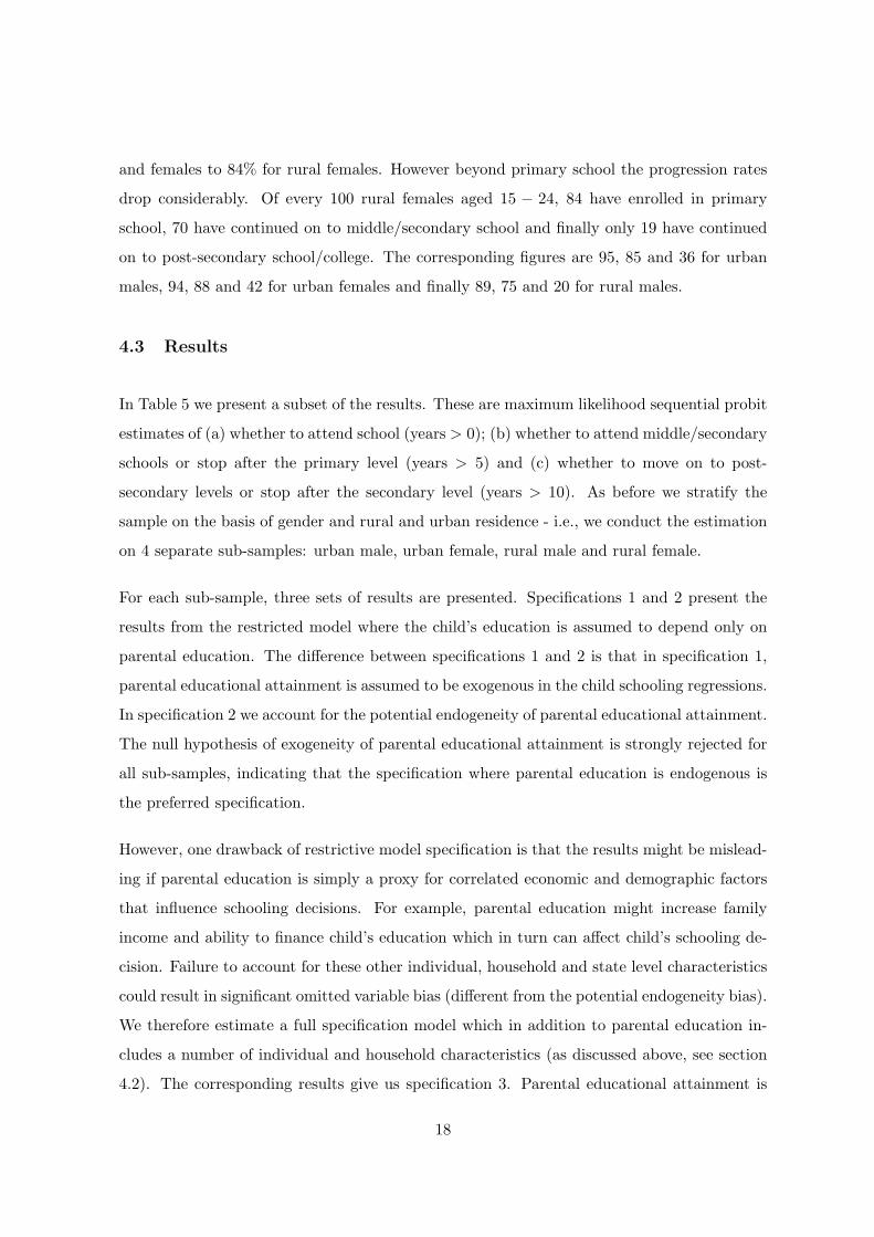
4.2 Specification, Data and Descriptive Statistics

The focus of our paper is to examine the intergenerational transmission of education. This

is captured by looking at the effect of years of schooling attained by the father and mother

on the educational attainment of the child (school progression to be more specific). We

correct for the potential endogeneity of parental educational attainment in the child schooling

regressions using the methodology developed by Rivers and Vuong (1988). The procedure

can be described as follows. First years of schooling attained by the father and mother are

regressed on the full set of explanatory variables including the instruments. This is the first

stage regression. The error terms from the first stage regression (Residual Father’s schooling

and Residual Mother’s schooling) are included as additional regressors in the second stage

estimation (the sequential probit model). Joint significance of the two residuals (LR =

−2(LR − LU ) ∼ χ2(6), where LR and LU are the restricted and unrestricted log likelihood

values) implies that the null hypothesis of exogeneity of parental educational attainment on

the child’s educational attainment is rejected. The estimation results show that the null

hypothesis of exogeneity of parental educational attainment is strongly rejected. As before

we use as instruments the year of birth of the father and mother and year of birth of the

father and mother × original location of the father and mother.

16

The other explanatory variables that we use in the regressions include individual and house-

hold level characteristics. Individual (child level) characteristics include the age of the child

and the number and composition of siblings. We compute and present separate results for

males and females and also by rural or urban residence. We include both the age of the child

and the square of the age of the child to account for any non-linearity in the age effect. These

two age terms also allow us to account for any birth cohort effects. To examine whether there

is a quantity-quality trade-off (Becker and Lewis, 1973) in educational attainment we include

the number of co-resident siblings for each child. However since the age and the gender of

the siblings could be important, we stratify the number of siblings by age and gender: the

number of brothers and sisters in the age group 0− 5, 6− 10, 11− 14 and 15− 24. It has been

argued that sibling composition may play an important role in a child’s school participation,

particularly if the child comes from a poor resource constrained household. This classification

of siblings therefore takes account of whether there is competition for the limited household

resources in schooling decisions. We will return to this issue below. We include the number of

working age males and females (aged 25−60) in the household; dummies for religion (Muslim,

Christian and Other religion; the reference category being Hindu), a dummy to indicate if

the household is below the poverty line and finally a set of province dummies to account for

any unobserved public investment (including state policy) that might have an effect on child

educational attainment. The estimation results show that the null hypothesis of exogeneity

of parental educational attainment is strongly rejected.

The descriptive statistics are presented in Columns (5) and (6) in Table 1 (corresponding

to Sample 3) for the rural and urban households respectively. Despite the fact that a large

fraction of the sample (37% in the rural areas and 51% in the urban areas) are in school at

the time of the survey and have essentially not completed their educational attainment, the

average years of schooling are much higher compared to sample of adults: 7.57 years and

9.51 years in the rural and urban households respectively, compared to 4.34 years and 7.69

years for the sample of adults. Interestingly 63% of the rural sample of 15− 24 year olds are

male. We cannot be sure if this is simply a sampling bias or the reflection of a much deeper

problem.

Figure 5 gives us an indication of the extent of the problem of school progression in India.

Enrolment rates among the 15−24 year olds is quite high, ranging from 94% for urban males

17

and females to 84% for rural females. However beyond primary school the progression rates

drop considerably. Of every 100 rural females aged 15 − 24, 84 have enrolled in primary

school, 70 have continued on to middle/secondary school and finally only 19 have continued

on to post-secondary school/college. The corresponding figures are 95, 85 and 36 for urban

males, 94, 88 and 42 for urban females and finally 89, 75 and 20 for rural males.

4.3 Results

In Table 5 we present a subset of the results. These are maximum likelihood sequential probit

estimates of (a) whether to attend school (years > 0); (b) whether to attend middle/secondary

schools or stop after the primary level (years > 5) and (c) whether to move on to post-

secondary levels or stop after the secondary level (years > 10). As before we stratify the

sample on the basis of gender and rural and urban residence - i.e., we conduct the estimation

on 4 separate sub-samples: urban male, urban female, rural male and rural female.

For each sub-sample, three sets of results are presented. Specifications 1 and 2 present the

results from the restricted model where the child’s education is assumed to depend only on

parental education. The difference between specifications 1 and 2 is that in specification 1,

parental educational attainment is assumed to be exogenous in the child schooling regressions.

In specification 2 we account for the potential endogeneity of parental educational attainment.

The null hypothesis of exogeneity of parental educational attainment is strongly rejected for

all sub-samples, indicating that the specification where parental education is endogenous is

the preferred specification.

However, one drawback of restrictive model specification is that the results might be mislead-

ing if parental education is simply a proxy for correlated economic and demographic factors

that influence schooling decisions. For example, parental education might increase family

income and ability to finance child’s education which in turn can affect child’s schooling de-

cision. Failure to account for these other individual, household and state level characteristics

could result in significant omitted variable bias (different from the potential endogeneity bias).

We therefore estimate a full specification model which in addition to parental education in-

cludes a number of individual and household characteristics (as discussed above, see section

4.2). The corresponding results give us specification 3. Parental educational attainment is

18

assumed to be endogenous in this specification.10 Also we report only the coefficient esti-

mates of father’s and mother’s education in Table 5. The full set of results are presented in

the Appendix (Table A-1). Two other points are worth noting. First the additional controls

are jointly statistically significant (χ2(111), see Table 5); and second the extent of omitted

variable bias is considerable (compare specifications 2 and 3 in Table 5). We come back to

this issue below.

Heterogeneity in the propensity to continue in school (captured by σ2δ ), which is assumed

to capture all correlation across schooling decisions, is always statistically significant. There

is a common individual level unobserved factor that affects schooling decision at every level

and ignoring this common individual level unobserved heterogeneity would result in biased

estimates. The extent of this bias becomes clear once we compare the effects of parental

educational attainment on school progression in the three specifications.

Parental Education Effect

The issue of endogeneity of parental educational attainment turns out to be fairly crucial

and it is important to note that the effects of parental educational attainment on the school

progression propensities are quite different in the three specifications. In the restricted mod-

els (specifications 1 and 2), both the years of schooling attained by the father and the years

of schooling attained by the mother always have a positive and statistically significant effect

on the continuation probabilities. However the effects vary across the different transitions

once we account for the potential endogeneity of parental education. Comparing the results

from specifications 1 and 2 we find that failing to account for endogeneity of parental ed-

ucational attainment results in an over estimation of the effect of the father’s educational

attainment on school enrolment, but an under estimation of the probability of continuing (or

propensity to continue) on to the middle/secondary school and post-secondary school/college.

The effect of the mother’s educational attainment follows the exact opposite pattern: failing

to account for endogeneity of mother’s educational attainment under estimates the effect of

mother’s educational attainment on the probability of enrolment, but over estimates the ef-

fect on the probability of continuation to middle/secondary school level and to post-secondary10The corresponding results for exogenous specification are presented in the Appendix (Table A-1).

19

school/college level.

The results from specification 3 are quite different. First, father’s education does not have

a statistically significant effect on the propensity to enrol in school; mother’s educational

attainment is positive and statistically significant. This result is true irrespective of the

gender of the child and irrespective of the sector of residence (rural or urban). However when

we compare the results from specifications 2 and 3 we find evidence of significant omitted

variable bias: over estimation of the effect of the father’s educational attainment and an

under estimation of the effect of the mother’s educational attainment.

Moving on to transition 2 (continuing to middle/secondary school, conditional on completing

primary school) we find that again with the exception of urban males, the father’s educa-

tional attainment does not have a statistically significant effect on the conditional probability

of attending middle/secondary school. Mother’s educational attainment on the other hand

has a positive and statistically significant effect on the conditional probability of attending

middle/secondary school, though not for urban males. Again a comparison of the estimates

in the three specifications shows that with the exception of the sub sample of urban males,

ignoring the control variables results in significant over estimation of the effect of the father’s

educational attainment on the propensity that the child attends middle/secondary effect while

it results in a significant under estimation of the effect of mother’s educational attainment on

the corresponding probability. For the sub-sample of urban males however the effects are the

opposite: ignoring control variables results in an under estimation of the effect of the father’s

education but an over estimation of the effect of the mother’s education.

Finally when we move to transition 3 (continuing on to post-secondary education), we find

that mother’s educational attainment ceases to have a statistically significant effect on the

probability of continuing on to post-secondary levels; on the other hand father’s education is

now positive and statistically significant.

It is important to note that the relative importance of the father’s and mother’s educational

attainment changes as children move from primary to middle/secondary to post-secondary

levels. We can calculate the change in probability of schooling due to an additional year of

parental education. The changes in probability (computed using the estimated coefficients

20

in Specification 3) are reported in Figure 6. An additional year of schooling attained by the

mother increases the probability of school enrolment by 2.2% for urban females and 4.3%

for rural females. The corresponding figures for urban and rural males are 3.2% and 4.2%

respectively. Similarly the likelihood of enrolling in middle school increases by 6.7% for urban

females and 8.3% for rural females with an additional year of their mothers schooling.11 These

results imply that mother’s education is more important for rural females relative to urban

females. Fathers education has almost no effect on school enrolment and continuation on to

middle/secondary school except in the case of urban males. However, an additional year of

father’s education increases the probability of progression to post-secondary school/college

with the effect being higher in urban areas. We come back to a possible explanation and

some implications of this result later.

These results are important from a policy point of view: clearly mother’s education is impor-

tant at the initial levels (decision whether to attend school in the first place or the decision on

whether to attend middle/secondary school, conditional on successful completion of primary

school (the latter effect though breaks down for the sample of urban males). At either of these

two transitions, father’s educational attainment has almost no role to play. However father’s

educational attainment becomes crucial in the decision to continue on to post-secondary lev-

els. This variation in effects is not evident if we do not account for endogeneity and other

household socio-economic characteristics. So if the focus of policy makers is to increase school

enrolment in the first place (as is the policy focus in large sections of the country), they need

to target the mothers. On the other hand if the focus is to ensure that children continue on to

post-secondary levels (may be to obtain technical training), policy makers need to target the

fathers and to the extent that the father’s educational attainment is a proxy for his income,

private investment continues to be important.12

Other Results

The full set of results are presented in Table A-1 in the Appendix. While not the primary

focus of the paper we discuss some of the more interesting results. Irrespective of the spec-11These numbers have been computed using the methodology developed by Petersen (1985).12This effect becomes even clearer when we compare the estimates of the years of schooling of the father

and the mother in the exogenous and endogenous specifications, presented in Table A-1 in the Appendix.

21

ification, the sample and the level, the Poor dummy is always negative and statistically

significant. This implies that children belonging to poor households (those below the poverty

line) are significantly less likely to enrol in school, significantly less likely to continue on to

middle/secondary school and significantly less likely to continue beyond secondary school (to

post-secondary school/college). There is therefore evidence of significant resource constraints

within the household, which is reflected in sub-optimal investment in schooling. Schooling

has costs in India. Even apparently free government schooling has substantial costs, such as

expenditure on books, stationery, travel, and school uniforms. The PROBE report (PROBE,

1999) found that, in rural north India, parents spend about Rs. 318 per year per child who

attends government (i.e., tuition-free) school, so that an agricultural laborer in Bihar with

three such children would have to work for about 40 days of the year just to send the children

to primary school (see Kingdon, 2005).

Resource constraints within the household manifest themselves in other ways as well. The

most important of which is the sibling competition or sibling rivalry effect.13 The idea is that

given resource constraints within the household, siblings compete among themselves over

resources, both parental time and money resources (see for example Mulder, 1998; Green-

halgh, 1985) and this has implications for human capital accumulation within the household.

Sibling gender composition has an important influence on intrahousehold resource allocation

of schooling and health resources, particularly if the child comes from a poor, resource-

constrained household. For example, if there is a gender bias operating at the household

level, then for a given family size, it must be the case that a male child, growing up in a

household with only brothers, may have fewer resources than if he were to grow up with

sisters only. This is likely to be true for females as well. This would imply that the educa-

tional attainment of children depends not only on their own gender but also on whether their

siblings are female or male. Hence, siblings become rivals in a competition for greater access

to household resources. We find that irrespective of the gender of the child and the region

of residence, an increase in the number of brothers or sisters aged 0− 10 always reduces the

probability of enrolling in school, continuing on to middle/secondary school and continuing

beyond secondary school for the 15− 24 year olds. The effects are in most cases statistically

significant. These results are consistent with the argument that elder siblings in resource13We ignore the issue of endogeneity of the number of siblings here.

22

constrained households have to leave school in order to take care of their siblings. What is

interesting is that the results are quite similar across gender.

The effects are however quite varied if there is an increase in the number of siblings aged

11 − 24. Having an additional brother in this age group reduces the probability of enrolling

in school, continuing on to middle/secondary school and continuing beyond secondary school.

This is true for both boys and girls. However having an additional sister in this age group

actually increases the corresponding probabilities at every level. It is worth noting however

that the effects of having an additional sister aged 11 − 24 is much weaker for continuation

to middle/secondary school and continuation beyond secondary school. The results then

imply that having a sister around the same age is actually beneficial for both boys and girls.

In this case appears to be no sibling competition effect − rather we seem to find evidence

of what could be termed as the sibling synergy effect. The results are consistent with the

hypothesis that older children may subsidize the education of younger siblings by contributing

to family time or budget. At transition 2 (continuation to middle/secondary school), only

older sisters in the age group of 15 − 24 years significantly increase the probability that

the younger brothers and sisters continue on to middle/secondary school. The effect of older

sisters on school enrolment is independent of the gender composition of the siblings. However,

at transition 3 (continuation to post-secondary school/college) the effect of older sisters (in

the age group of 15 − 24) remains significant only for siblings of the same gender. This

leads to two interesting observations. First, school enrolment is affected by both categories

of older sisters: the 11 − 15 year olds who are more likely to contribute to family time and

the 15− 24 year olds who are more likely to contribute to family budget, whereas progression

across schooling levels is significantly affected by only one category of older sisters; ones who

are more likely to contribute financially to family budget. Second, females are more likely

to continue beyond middle/secondary school if they have an elder sister in the age group of

15−24: again a reflection of the sibling synergy effect. There is therefore a positive spill over

effect from having children attend school, due to economies of scale in child costs and/or from

the development of a culture of schooling within the household influenced by social forces.

The spill over essentially results in a form of positive externality in children’s educational

attainment, which the parents will try to internalize through their schooling decisions for

subsequent (other) children. Thus rather than the standard sibling competition effect we

23

find a sibling synergy effect, making it optimal for parents to educate a greater number of

children.14

The effect of an additional working age male is never statistically significant. However, an

additional working age female in the household has a significant and positive effect on school

enrolment and progression of all children in the household. This is not surprising and is partly

a reflection of the fact that in developing countries one of the most important reasons as to

why children drop out of school is that they need to help with household chores. Having

an additional working age woman in the household clearly makes things easier. Our results

show significant heterogeneity in schooling among children from different religions. Muslim,

Christian and other religion children have reduced likelihood of enrolment in school, relative

to Hindu students. Even conditional on enrolment children from Muslim households are less

likely to progress beyond primary school. Conditional on enrolment however the results are

more positive for Christian children and children belonging to other religions.

5 Concluding Remarks

Investment in human capital through education is universally recognized as an essential com-

ponent of economic development. While education endows individuals with the means to

enhance their skills, knowledge, health and productivity, it also enhances the economy’s abil-14While the issue of sibling competition effect is fairly well established result in the context of developed

countries (see for example Behrman et al. (1989) and Conley and Glauber (2006) for the US and Gouxand Maurin (2004) for France), evidence using data from developing countries is quite mixed. Evidence fromThailand (Knodel et al., 1990) and Brazil (Psacharopoulos and Arriagada, 1989) suggest that there is a negativerelationship between the number of siblings and educational attainment. In the case of Vietnam (Anh et al.,1998) the relationship is negative for families with six or more children and the effects are quite small once otherfamilies are controlled for. In the context of Indonesia, Malarani (2004) finds that the relationship betweenfamily size and schooling was positive or neutral for the older cohorts, but for the younger cohorts there is anegative relationship. Qian (2009), using data from China, provides causal evidence of benefit of an additionalsibling to first born children. She finds that for one-child families, an additional child significantly increasesthe school enrolment of the first born. Using data from Taiwan, Parish and Willis (1993) and Greenhalgh(1985) find that where children with relatively more older sisters have higher schooling rates. Shavit andPierce (1991), using data from Israel find that for the richer Jews, family size has a negative relationship witheducational attainment of children, while there is a positive relationship between family size and educationalattainment of children in the poorer Muslim households. In African countries, however, there is no negativeeffect and in fact the opposite is true: educational attainment has a positive relationship with the number ofsiblings (see Gomes (1984) for evidence from Kenya; Chernichovsky (1985) for evidence from Botswana; andCornwell et al. (2007) for evidence from South Africa). The explanation for this positive relationship typicallyinvolves households in Africa (and indeed the poor Muslim communities in Israel) drawing on a large kinshipnetwork beyond the immediate family, which reduces the costs (financial, emotional and time) associated withadditional children.

24

ity to develop and adopt new technology. Not surprisingly therefore, increasing education

levels is an important policy concern in most countries.

The primary purpose of this paper is to look at the association between parental education

and children’s education. Educational attainment of any individual depends on both private

and public investments. Parental educational attainment is the prime component of the

former. In the extreme case where the society is completely rigid, children’s educational

attainment is determined completely by parental educational attainment. All that matters

is private investment. But that also means that the distributional impacts of growth could

be negative, since a large section of the population will not be able to accumulate the human

capital necessary to reap the benefits of the process of economic growth.

There are three main results of this paper. First, we find that in India there has been a

significant increase in educational attainment of individuals over the last 70 years or so with

women gaining the most in terms of increases in educational attainment. Second, restricting

the sample to adults (those more than 20 years old at the time of the survey), we find that

when we account for the potential endogeneity of parental educational attainment, it is public

investments in education that matters and not private investments. Educational attainment

of the next generation is not constrained by the endowments, preferences and opportunities

provided by the previous generation and that state policy has been successful in severing

this link. Ignoring the potential endogeneity of parental educational attainment significantly

over estimates the effect of parental educational attainment on the educational attainment of

adults. Finally, the sequential probit analysis of school progression (for the 15− 24 year olds

at the time of the survey) shows that the effect of parental education on school progression

varies over the different stages. Mother’s education is important at the initial transitions

− decision whether to attend school in the first place or the decision on whether to attend

middle/secondary school, conditional on successful completion of primary school (the latter

effect though surprisingly breaks down for the sample of urban males). At either of these

two transitions, father’s educational attainment has almost no role to play. However father’s

educational attainment becomes crucial in the decision to continue on to post-secondary

levels. This variation in effects is not evident if we do not account for endogeneity of parental

education. So if the focus of policy makers is to increase school enrolment in the first place (as

is the policy focus in large sections of the country), they need to target the mothers. On the

25

other hand if the focus is to ensure that children continue on to post-secondary levels (may

be to obtain technical training), policy makers need to target the fathers. These results are

a distinct improvement over the existing univariate probit or ordered probit estimates of the

highest educational attainment as they allow us to account for selection at the different levels

and also shows (i) how different characteristics affect school progression differently at the

different stages and (ii) how the same set of factors might affect different levels of schooling

in a different manner.

Controlling for endogeneity weakens the direct effect of fathers education on school enrolment

and on continuation beyond primary school schooling and mothers education on continua-

tion beyond middle/secondary school. However conditional on the child continuing beyond

primary school, father’s educational attainment has a significant effect on progression to

post-secondary school/college. This result is consistent with the existing hypothesis in the

literature that the direct effect of fathers education results from its impact on the household

income and resources (market factors). Thus the decision to send a child to post-secondary

school/college is primarily determined by household income. In contrast the direct effect of

mothers education is associated with non-market factors such as awareness about education

and quality of time she spends with children. Our result of positive and significant effect of

mothers education at initial stages of schooling is consistent with the above hypothesis.

Over the long run (and after accounting for the potential endogeneity of parental educational

attainment) we find that there has been a significant increase in intergenerational educa-

tional mobility in India. These results also imply that it is public investments in education

and not private investments that matters. Educational attainment of the next generation is

not constrained by the endowments, preferences and opportunities provided by the previous

generation and that state policy has been successful in severing this link. This is a positive

result and is not particularly surprising. Over the last 70 years the rate of growth of educa-

tional infrastructure has far exceeded the rate of growth of parental educational attainment.

It is therefore logical that the effect is dominated by the supply side variable: a clear case

of if you build it they will come. The main result from school progression analysis is that

father’s educational attainment has a positive and statistically significant effect on the proba-

bility of continuing to post-secondary school/college. To the extent that father’s educational

attainment is a proxy for his income, these results seem to suggest that the probability of

26

continuing to post-secondary schooling is positively affected by the father’s income (which

one would think is the primary determinant of private investment in schooling).15 Given that

a large part of the Indian growth process over the last 2 decades has been driven by the highly

skilled Information Technology sector, continuation to post-secondary school/college (in or-

der to accumulate the necessary technical skills) is crucial to benefit from the opportunities

offered by the Indian growth process. In this respect private investment (driven primarily by

father’s income) continues to be crucial.

15It is worth noting that the “poor” dummy is always negative and statistically significant: it is the father’sincome that matters and not overall household income. This is not surprising. In India where most householdsare not nuclear, it is likely that income from different sources and accruing to different individuals have differentuses; child’s education is the responsibility of the father.

27

References

Anh, T. S., J. Knodel, D. Lam, and J. Friedman (1998). Family Size and Childrens Education in Vietnam.Demography 35 (1), 57 – 70.

Barro, R. (2001). Human capital and growth. American Economic Review , 12–17.

Becker, G., K. Murphy, and R. Tamura (1990). Human capital, fertility, and economic growth. Journal ofPolitical Economy , 12–37.

Becker, G. and N. Tomes (1986). Human capital and the rise and fall of families. Journal of Labor Economics,1–39.

Becker, G. S. and H. G. Lewis (1973). Interaction between quantity and quality of children. Journal of PoliticalEconomy 81 (2), S279 – S288.

Behrman, J., N. Birdsall, and M. Szekely (2000). Intergenerational Mobility in Latin America: Deeper Marketsand Better Schools Make a Difference, pp. 135 – 167. Washington DC: Brookings Institution.

Behrman, J. and M. Rosenzweig (2002). Does increasing women’s schooling raise the schooling of the nextgeneration? American Economic Review 92 (1), 323–334.

Behrman, J. R., A. Pollak, and P. Taubman (1989). Child Endowments and the Quantity and Quality ofChildren. Journal of Political Economy 97 (2), 389 – 419.

Bourguignon, F., F. Ferreira, and M. Menendez (2003). Inequality of outcomes and inequality of opportunitiesin brazil. Technical Report 3174, World Bank Policy Research Working Paper.

Chernichovsky, D. (1985). Socioeconomic and Demographic Aspects of School Enrolment and Attendance inRural Botswana. Economic Development and Cultural Change 33, 319 – 332.

Conley, D. and R. Glauber (2006). Parental Educational Investment and Children’s Academic Risk: Estimatesof the Impact of Sibship Size and Birth Order from Exogenous Variation in Fertility. Journal of HumanResources XLI (4), 722 – 735.

Cornwell, K., B. Inder, P. Maitra, and A. Rammohan (2007). Household composition and schooling of ruralsouth african children: Sibling synergy and migrant effects. Technical report, Monash University, Australia.

Dreze, J. and G. Kingdon (2001). School Participation in Rural India. Review of Development Economics 5 (1),1–24.

Gau, W. and R. Smyth (2009). Health Human Capital, Height and Wages in China. Journal of Developmentstudies Forthcoming.

Gomes, M. (1984). Family Size and Educational Attainment in Kenya. Population and Development Review 10,647 – 660.

Goux, D. and E. Maurin (2004). The Effects of Overcrowded Housing on Childrens Performance at School.CEPR Discussion Paper # 3818 .

Greenhalgh, S. (1985). Sexual stratification: The other side of” growth with equity” in east Asia. Populationand Development Review , 265–314.

Gupta, D. (2004). Caste. Oxford: Oxford University Press.

Holmes, J. (2003). The determinants of completed schooling in pakistan: Analysis of censoring and selectionbias. Economics of Education Review 22, 249 – 264.

Jalan, J. and R. Murgai (2008). Intergenerational mobility in education in india. Technical report, PaperPresented at the Indian Statistical Institute, Delhi.

28

Kingdon, G. G. (2005). Where has all the bias gone? Detecting gender bias in the Intra-household Allocationof Educational Expenditure. Economic Development and Cultural Change 53 (2), 409 – 452.

Kingdon, G. G. (2007). The progress of school education in India. Oxford Review of Economic Policy 23 (2),168 – 195.

Knodel, J., N. Havanon, and W. Sittirai (1990). Family Size and the Education of Children in the Context ofRapid Fertility Decline. Population and Development Review 16, 31 – 62.

Lillard, L. and R. J. Willis (1994). Intergenerational educational mobility: Effects of family and state inmalaysia. Journal of Human Resources 29 (4), 1126–1167.

Maitra, P. (2003). Schooling and educational attainment: Evidence from bangladesh. Education Eco-nomics 11 (2), 129 – 153.

Malarani, V. (2004). Family size and educational attainment in indonesia: A cohort perspective. Technicalreport, California Center for Population Research, University of California, Los Angeles.

Mulder, M. (1998). Brothers and sisters. Human Nature 9 (2), 119–161.

Munshi, K. and M. R. Rosenzweig (2009). Why is mobility in india so low? social insurance, inequality andgrowth. Technical report, Brown University.

Pal, S. (2004). Child schooling in peru: Evidence from a sequential analysis of school progression. Journal ofPopulation Economics 17 (4), 657–680.

Parish, W. and R. Willis (1993). Daughters, education, and family budgets Taiwan experiences. Journal ofHuman Resources, 863–898.

Petersen, T. (1985). A comment on presenting results from logit and probit models. American SociologicalReview , 130–131.

PROBE (1999). Public Report on Basic Education in India. Delhi: Oxford University Press.

Psacharopoulos, G. and A. M. Arriagada (1989). The Determinants of Early Age Human Capital Formation:Evidence from Brazil. Economic Development and Cultural Change 37, 683 – 708.

Qian, N. (2009). Quantity-quality and the one child policy:the only-child disadvantage in school enrollment inrural china. Technical report, NBER Working Papers #14973, National Bureau of Economic Research, Inc.

Rivers, D. and Q. H. Vuong (1988). Limited information estimators and exogeneity tests for simultaneousprobit models. Journal of Econometrics 39, 347 – 366.

Rosenzweig, M. and K. Wolpin (1994). Are there increasing returns to the intergenerational production ofhuman capital? Maternal schooling and child intellectual achievement. Journal of Human Resources, 670–693.

Schultz, T. (2002). Wage gains associated with height as a form of health human capital. American EconomicReview , 349–353.

Shavit, Y. and J. L. Pierce (1991). Sibship Size and Educational Attainment in Nuclear and Extended Families:Arabs and Jews in Israel. American Sociological Review 56, 321 – 330.

Singh, R. (1992). Underinvestment, low economic returns to education, and the schooling of rural children:some evidence from Brazil. Economic Development and Cultural Change, 645–664.

Spierings, J. (1999). A crucial point in life: learning, work and young adults. australia’s young adults: thedeepening divide. Technical report, Dusseldorp Skills Forum: 5-27.

Thomas, D. (1996). Education across generations in south africa. American Economic Review, Papers andProceedings 86 (2), 330 – 334.

UN (1999). World population ageing 1950-2050. UN.

29

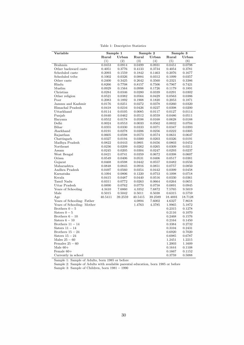
Table 1: Descriptive Statistics

Variable Sample 1 Sample 2 Sample 3Rural Urban Rural Urban Rural Urban

(1) (2) (3) (4) (5) (6)Brahmin 0.0453 0.0914 0.0499 0.0931 0.0451 0.0798Other backward caste 0.4051 0.3776 0.4133 0.3734 0.4054 0.3781Scheduled caste 0.2093 0.1559 0.1842 0.1463 0.2076 0.1677Scheduled tribe 0.1002 0.0326 0.0884 0.0312 0.1099 0.0357Other caste 0.2400 0.3425 0.2642 0.3560 0.2321 0.3386Hindu 0.8266 0.7708 0.8157 0.7506 0.7967 0.7421Muslim 0.0929 0.1564 0.0998 0.1726 0.1179 0.1891Christian 0.0284 0.0346 0.0280 0.0339 0.0291 0.0302Other religion 0.0521 0.0382 0.0564 0.0429 0.0563 0.0386Poor 0.2083 0.1892 0.1908 0.1820 0.2053 0.1871Jammu and Kashmir 0.0176 0.0251 0.0272 0.0378 0.0260 0.0320Himachal Pradesh 0.0418 0.0216 0.0426 0.0227 0.0398 0.0200Uttarkhand 0.0114 0.0105 0.0085 0.0117 0.0127 0.0114Punjab 0.0440 0.0462 0.0512 0.0559 0.0486 0.0511Haryana 0.0552 0.0178 0.0598 0.0168 0.0628 0.0188Delhi 0.0024 0.0553 0.0033 0.0562 0.0032 0.0704Bihar 0.0355 0.0330 0.0333 0.0371 0.0347 0.0393Jharkhand 0.0191 0.0278 0.0206 0.0256 0.0222 0.0305Rajasthan 0.0605 0.0598 0.0573 0.0574 0.0631 0.0647Chattisgarh 0.0327 0.0194 0.0300 0.0203 0.0326 0.0191Madhya Pradesh 0.0822 0.0443 0.0801 0.0456 0.0803 0.0452Northeast 0.0236 0.0209 0.0262 0.0265 0.0309 0.0211Assam 0.0245 0.0205 0.0304 0.0247 0.0293 0.0237West Bengal 0.0421 0.0741 0.0359 0.0672 0.0398 0.0607Orissa 0.0549 0.0406 0.0531 0.0406 0.0517 0.0381Gujarat 0.0468 0.0598 0.0442 0.0557 0.0482 0.0556Maharashtra 0.0848 0.0845 0.0916 0.0851 0.0757 0.0850Andhra Pradesh 0.0497 0.0560 0.0354 0.0442 0.0399 0.0458Karnataka 0.1094 0.0806 0.1220 0.0753 0.1098 0.0718Kerala 0.0415 0.0487 0.0440 0.0516 0.0330 0.0361Tamil Nadu 0.0311 0.0772 0.0263 0.0664 0.0264 0.0651Uttar Pradesh 0.0890 0.0762 0.0770 0.0758 0.0891 0.0945Years of Schooling 4.3410 7.6860 4.3352 7.6872 7.5765 9.5019Male 0.5015 0.5042 0.5011 0.5038 0.6315 0.5759Age 40.5411 39.2559 40.5415 39.2589 18.4693 18.7128Years of Schooling: Father 4.0894 7.6002 4.6327 7.8618Years of Schooling: Mother 1.4763 4.3785 1.9965 5.1872Brothers 0− 5 0.2315 0.1278Sisters 0− 5 0.2116 0.1070Brothers 6− 10 0.2468 0.1576Sisters 6− 10 0.2164 0.1450Brothers 11− 14 0.3384 0.2732Sisters 11− 14 0.3104 0.2431Brothers 15− 24 0.6920 0.7020Sisters 15− 24 0.6985 0.6787Males 25− 60 1.2451 1.2215Females 25− 60 1.2003 1.1609Male 60+ 0.1644 0.1108Female 60+ 0.1667 0.1152Currently in school 0.3759 0.5088

Sample 1: Sample of Adults, born 1985 or beforeSample 2: Sample of Adults with available parental education, born 1985 or beforeSample 3: Sample of Children, born 1981− 1990

30

Table 2: Levels and Growth of in Educational Attainment of Adults

Urban Male Urban Female Rural Male Rural Female(1) (2) (3) (4)

Panel AYears of Schooling (OLS) 0.0528*** 0.1219*** 0.1025*** 0.1011***

(0.0021) (0.0020) (0.0012) (0.0012)Sample Mean 8.8035 6.5496 5.6779 2.9961Observations 21959 21592 40196 39954Panel BEnrolled in School (Marginal Effects) 0.0026*** 0.0084*** 0.0076*** 0.0159***

(0.0001) (0.0002) (0.0001) (0.0002)Sample Mean 0.8727 0.7492 0.3481 0.2163Observations 29973 29079 56875 55601Panel CEnrolled in Middle School (Marginal Effects) 0.0024*** 0.0055*** 0.0069*** 0.0101***

(0.0001) (0.0002) (0.0001) (0.0003)Sample Mean 0.6979 0.5605 0.2295 0.1369Observations 22800 18486 34718 21782Panel DEnrolled in Post-Secondary School (Marginal Effects) 0.0022*** 0.0070*** 0.0046*** 0.0075***

(0.0003) (0.0004) (0.0003) (0.0005)Sample Mean 0.6948 0.4988 0.1465 0.0647Observations 16452 12102 20051 10217Panel EEnrolled in College (Marginal Effects) -0.0017*** 0.0007 -0.0007 -0.0007

(0.0005) (0.0008) (0.0007) (0.0016)Sample Mean 0.4041 0.2557 0.0573 0.0241Observations 6127 3457 4304 1239

Notes:∗∗∗p < 0.01,∗∗ p < 0.05,∗ p < 0.1Standard errors clustered at the household levelAdults defined as born in 1985 or earlier

31

Tab

le3:

Lev

els

and

Gro

wth

ofin

Edu

cati

onal

Att

ainm

ent

ofA

dult

s:by

Rel

igio

nan

dC

aste

All

Hin

du

Musl

imC

hris

tian

Oth

er

Religio

nB

rahm

inO

BC

SC

ST

Oth

er

Cast

e(1

)(2

)(3

)(4

)(5

)(6

)(7

)(8

)(9

)(1

0)

Urban

Male

sG

row

thp

eryea

r0.0

528***

0.0

571***

0.0

563***

0.0

472***

0.0

545***

0.0

397***

0.0

710***

0.0

895***

0.0

755***

0.0

378***

(0.0

021)

(0.0

024)

(0.0

049)

(0.0

100)

(0.0

098)

(0.0

052)

(0.0

033)

(0.0

051)

(0.0

121)

(0.0

034)

Sam

ple

mea

n8.8

09.1

76.4

99.9

410.0

611.5

98.1

17.1

18.2

49.6

5S

am

ple

size

21959

16945

3463

730

821

2010

8300

3408

706

7535

Urban

Fem

ale

sG

row

thp

eryea

r0.1

219***

0.1

254***

0.1

255***

0.1

070***

0.1

437***

0.1

349***

0.1

332***

0.1

344***

0.1

316***

0.1

153***

(0.0

020)

(0.0

023)

(0.0

047)

(0.0

102)

(0.0

090)

(0.0

058)

(0.0

030)

(0.0

047)

(0.0

126)

(0.0

035)

Sam

ple

mea

n6.5

56.7

84.4

29.0

88.2

19.2

25.7

54.5

56.2

67.6

6S

am

ple

size

21592

16625

3347

777

843

1972

8143

3380

715

7382

RuralM

ale

sG

row

thp

eryea

r0.1

025***

0.1

058***

0.0

897***

0.0

720***

0.1

081***

0.0

983***

0.1

076***

0.1

133***

0.0

974***

0.1

003***

(0.0

012)

(0.0

014)

(0.0

040)

(0.0

074)

(0.0

050)

(0.0

054)

(0.0

019)

(0.0

025)

(0.0

040)

(0.0

025)

Sam

ple

mea

n5.6

85.7

24.8

97.3

65.5

78.9

75.7

04.6

14.0

46.6

5S

am

ple

size

40196

33180

3775

1109

2132

1796

16216

8463

4037

9684

RuralFem

ale

sG

row

thp

eryea

r0.1

011***

0.1

033***

0.0

823***

0.1

019***

0.1

203***

0.1

499***

0.1

029***

0.0

874***

0.0

754***

0.1

176***

(0.0

012)

(0.0

012)

(0.0

036)

(0.0

075)

(0.0

052)

(0.0

051)

(0.0

018)

(0.0

023)

(0.0

033)

(0.0

024)

Sam

ple

mea

n3.0

02.9

22.4

06.2

03.5

35.0

12.8

92.0

31.8

94.1

0S

am

ple

size

39954

33070

3669

1171

2044

1837

16255

8316

3994

9552

Note

s:∗∗∗p<

0.0

1,∗∗p<

0.0

5,∗p<

0.1

Sta

nd

ard

erro

rscl

ust

ered

at

the

hou

seh

old

level

Ad

ult

sd

efin

edas

born

in1985

or

earl

ier

32

Tab

le4:

Par

enta

lE

duca

tion

and

Chi

ldre

n’s

Edu

cati

on.

OL

San

dIn

stru

men

tal

Var

iabl

eR

egre

ssio

n

Urban

Male

Urban

Fem

ale

RuralM

ale

RuralFem

ale

OLS

IVR

eg

OLS

IVR

eg

OLS

IVR

eg

OLS

IVR

eg

(1)

(2)

(3)

(4)

(5)

(6)

(7)

(8)

Yea

rof

Bir

th-0

.0463***

-0.0

241

0.0

570***

0.0

660**

0.0

153***

0.0

154

0.1

518***

0.1

756***

(0.0

073)

(0.0

395)

(0.0

221)

(0.0

334)

(0.0

059)

(0.0

111)

(0.0

163)

(0.0

250)

Fath

er:

Yea

rsof

Sch

oolin

g0.3

332***

0.6

197

0.2

708***

-0.1

949

0.3

831***

-0.0

955

0.3

914***

0.2

562

(0.0

146)

(0.8

680)

(0.0

265)

(0.5

581)

(0.0

106)

(0.1

882)

(0.0

267)

(0.3

147)

Moth

er:

Yea

rsof

Sch

oolin

g0.1

308***

-0.4

940

0.2

047***

0.4

051

0.1

524***

0.7

752*

0.2

470***

0.1

374

(0.0

130)

(1.2

969)

(0.0

222)

(0.4

928)

(0.0

149)

(0.4

305)

(0.0

317)

(0.2

503)

Mu

slim

-1.5

454***

-2.2

743**

-1.0

155***

-1.4

475**

-1.0

505***

-1.0

397***

-1.1

199***

-1.3

564***

(0.1

579)

(1.0

710)

(0.3

221)

(0.6

671)

(0.1

517)

(0.2

114)

(0.3

791)

(0.4

177)

Ch

rist

ian

-0.8

051***

-0.0

212

-0.2

756

-0.1

304

-0.1

417

-0.7

105

0.6

057

0.7

845

(0.2

581)

(1.4

372)

(0.3

373)

(0.4

151)

(0.2

803)

(0.6

737)

(0.4

178)

(0.5

022)

Oth

erre

ligio

n-0

.3544

0.1

583

-0.2

407

0.1

678

-0.7

811***

-0.8

757***

-0.8

772*

-0.9

177*

(0.2

286)

(0.9

329)

(0.2

979)

(0.5

219)

(0.2

338)

(0.2

739)

(0.5

188)

(0.5

134)

Poor

-1.5

356***

-2.2

232***

-1.8

189***

-3.0

193***

-1.6

817***

-2.0

718***

-1.8

829***

-2.4

918***

(0.1

603)

(0.8

297)

(0.2

961)

(1.1

384)

(0.1

154)

(0.2

224)

(0.2

879)

(0.6

672)

Con

stant

98.7

989***

55.7

278

-105.6

707**

-120.2

461*

-23.6

804**

-22.2

034

-296.7

307***

-342.6

647***

(14.3

543)

(78.4

342)

(43.7

773)

(65.8

116)

(11.6

766)

(22.0

450)

(32.2

313)

(48.2

645)

Ob

serv

ati

on

s5789

5789

1886

1886

11515

11515

2078

2078

Han

sen

J-s

tati

stic

0.0

48

0.7

99

0.5

38

0.9

05

Sarg

an

Sta

tist

ic†

0.0

92

0.8

11

0.7

24

1.1

78

∗∗∗p<

0.0

1,∗∗p<

0.0

5,∗p<

0.1

Sta

nd

ard

erro

rscl

ust

ered

at

the

hou

seh

old

level

Reg

ress

ion

sin

clu

de

state

du

mm

ies.

Ref

eren

ceca

tegory

:h

ou

seh

old

resi

des

inU

ttar

Pra

des

h†

:S

arg

an

Sta

tist

ics

com

pu

ted

ass

um

ing

IID

erro

rst

ruct

ure

33

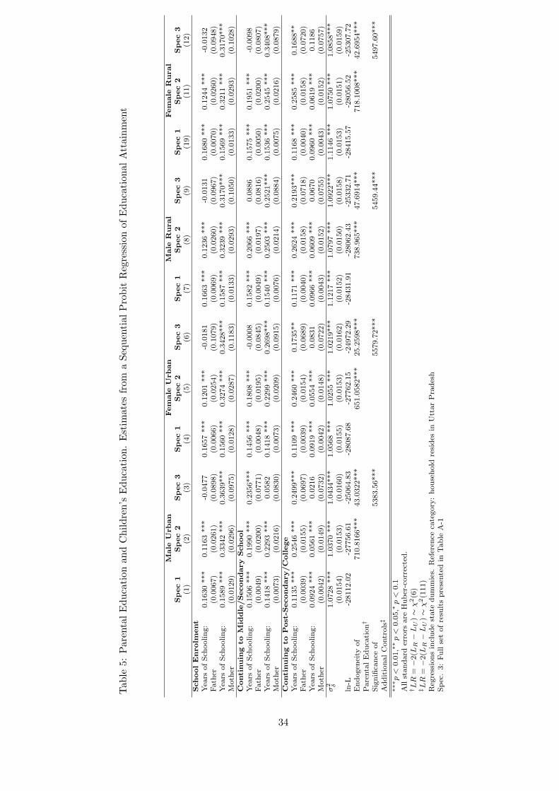
Tab

le5:

Par

enta

lE

duca

tion

and

Chi

ldre

n’s

Edu

cati

on.

Est

imat

esfr

oma

Sequ

enti

alP

robi

tR

egre

ssio

nof

Edu

cati

onal

Att

ainm

ent

Male

Urban

Fem

ale

Urban

Male

Rural

Fem

ale

Rural

Spec

1Spec

2Spec

3Spec

1Spec

2Spec

3Spec

1Spec

2Spec

3Spec

1Spec

2Spec

3(1

)(2

)(3

)(4

)(5

)(6

)(7

)(8

)(9

)(1

9)

(11)

(12)

SchoolEnrolm

ent

Yea

rsof

Sch

oolin

g:

0.1

630

***

0.1

163

***

-0.0

477

0.1

657

***

0.1

201

***

-0.0

181

0.1

663

***

0.1

236

***

-0.0

131

0.1

680

***

0.1

244

***

-0.0

132

Fath

er(0

.0067)

(0.0

261)

(0.0

898)

(0.0

066)

(0.0

254)

(0.1

079)

(0.0

069)

(0.0

260)

(0.0

967)

(0.0

070)

(0.0

260)

(0.0

948)

Yea

rsof

Sch

oolin

g:

0.1

589

***

0.3

342

***

0.3

639***

0.1

560

***

0.3

274

***

0.3

428***

0.1

587

***

0.3

239

***

0.3

170***

0.1

569

***

0.3

211

***

0.3

170***

Moth

er(0

.0129)

(0.0

296)

(0.0

975)

(0.0

128)

(0.0

287)

(0.1

183)

(0.0

133)

(0.0

293)

(0.1

050)

(0.0

133)

(0.0

293)

(0.1

028)

Conti

nuin

gto

Mid

dle

/Secondary

School

Yea

rsof

Sch

oolin

g:

0.1

506

***

0.1

990

***

0.2

356***

0.1

456

***

0.1

808

***

-0.0

008

0.1

582

***

0.2

066

***

0.0

886

0.1

575

***

0.1

951

***

-0.0

098

Fath

er(0

.0049)

(0.0

200)

(0.0

771)

(0.0

048)

(0.0

195)

(0.0

845)

(0.0

049)

(0.0

197)

(0.0

816)

(0.0

050)

(0.0

200)

(0.0

807)

Yea

rsof

Sch

oolin

g:

0.1

418

***

0.2

293

***

0.0

582

0.1

418

***

0.2

299

***

0.2

698***

0.1

540

***

0.2

503

***

0.2

521***

0.1

536

***

0.2

545

***

0.3

408***

Moth

er(0

.0073)

(0.0

216)

(0.0

830)

(0.0

073)

(0.0

209)

(0.0

915)

(0.0

076)

(0.0

214)

(0.0

884)

(0.0

075)

(0.0

216)

(0.0

879)

Conti

nuin

gto

Post

-Secondary/C

ollege

Yea

rsof

Sch

oolin

g:

0.1

135

***

0.2

546

***

0.2

499***

0.1

109

***

0.2

460

***

0.1

735**

0.1

171

***

0.2

624

***

0.2

193***

0.1

168

***

0.2

585

***

0.1

688**

Fath

er(0

.0039)

(0.0

155)

(0.0

697)

(0.0

039)

(0.0

154)

(0.0

689)

(0.0

040)

(0.0

158)

(0.0

718)

(0.0

040)

(0.0

158)

(0.0

720)

Yea

rsof

Sch

oolin

g:

0.0

924

***

0.0

561

***

0.0

216

0.0

919

***

0.0

554

***

0.0

831

0.0

966

***

0.0

609

***

0.0

670

0.0

960

***

0.0

619

***

0.1

186

Moth

er(0

.0042)

(0.0

149)

(0.0

732)

(0.0

042)

(0.0

148)

(0.0

722)

(0.0

043)

(0.0

152)

(0.0

755)

(0.0

043)

(0.0

152)

(0.0

757)

σ2 δ

1.0

728

***

1.0

370

***

1.0

434***

1.0

568

***

1.0

255

***

1.0

219***

1.1

217

***

1.0

797

***

1.0

922***

1.1

146

***

1.0

750

***

1.0

858***

(0.0

154)

(0.0

153)

(0.0

160)

(0.0

155)

(0.0

153)

(0.0

162)

(0.0

152)

(0.0

150)

(0.0

158)

(0.0

153)

(0.0

151)

(0.0

159)

ln-L

-28112.0

2-2

7756.6

1-2

5064.8

3-2

8087.6

8-2

7762.1

5-2

4972.2

9-2

8431.9

1-2

8062.4

3-2

5332.7

1-2

8415.5

7-2

8056.5

2-2

5307.7

2E

nd

ogen

eity

of

710.8

166***

43.0

322***

651.0

582***

25.2

598***

738.9

65***

47.6

914***

718.1

008***

42.6

954***

Pare

nta

lE

du

cati

on†

Sig

nifi

can

ceof

5383.5

6***

5579.7

2***

5459.4

4***

5497.6

0***

Ad

dit

ion

al

Contr

ols‡

∗∗∗p<

0.0

1,∗∗p<

0.0

5,∗p<

0.1

All

stan

dard

erro

rsare

Hub

er-c

orr

ecte

d.

† LR

=−

2(LR−LU

)∼χ

2(6

)‡ LR

=−

2(LR−LU

)∼χ

2(1

11)

Reg

ress

ion

sin

clu

de

state

du

mm

ies.

Ref

eren

ceca

tegory

:h

ou

seh

old

resi

des

inU

ttar

Pra

des

hS

pec

.3:

Fu

llse

tof

resu

lts

pre

sente

din

Tab

leA

-1

34

Figure 1: Average Years of Schooling by Cohort of Birth0

24

68

10Ye

ars

1 2 3 4 5 6 7 8 9 10 11 12 13 14

Urban Male

02

46

810

Year

s

1 2 3 4 5 6 7 8 9 10 11 12 13 14

Urban Female

02

46

810

Year

s

1 2 3 4 5 6 7 8 9 10 11 12 13 14

Rural Male

02

46

810

Year

s

1 2 3 4 5 6 7 8 9 10 11 12 13 14

Rural Female

Cohort 1 = Year of Birth ≤ 1930 Cohort 2 = Year of Birth > 1930 & Year of Birth ≤ 1935

Cohort 3 = Year of Birth > 1935 & Year of Birth ≤ 1940 Cohort 4 = Year of Birth > 1940 & Year of Birth ≤ 1945

Cohort 5 = Year of Birth > 1945 & Year of Birth ≤ 1950 Cohort 6 = Year of Birth > 1950 & Year of Birth ≤ 1955

Cohort 7 = Year of Birth > 1955 & Year of Birth ≤ 1960 Cohort 8 = Year of Birth > 1960 & Year of Birth ≤ 1965

Cohort 9 = Year of Birth > 1965 & Year of Birth ≤ 1970 Cohort 10 = Year of Birth > 1970 & Year of Birth ≤ 1975

Cohort 11 = Year of Birth > 1975 & Year of Birth ≤ 1980 Cohort 12 = Year of Birth > 1980 & Year of Birth ≤ 1985

Cohort 13 = Year of Birth > 1985 & Year of Birth ≤ 1990 Cohort 14 = Year of Birth > 1990 & Year of Birth ≤ 1995

35

Figure 2: Lowess Plot of Years of Schooling by Year of Birth0

24

68

10Y

ears

of S

choo

ling

1900 1910 1920 1930 1940 1950 1960 1970 1980 1990Year Born

Urban Males Urban FemalesRural Males Rural Females

36

Figure 3: Lowess Plot of Years of Schooling by Years of Schooling Attained by Father andMother

05

1015

Year

s of

Sch

oolin

g

0 5 10 15Years of Schooling of Father

45 degrees Urban MalesUrban Females Rural MalesRural Females

05

1015

Year

s of

Sch

oolin

g

0 5 10 15Years of Schooling of Mother

45 degrees Urban MalesUrban Females Rural MalesRural Females

37

Figure 4: Schematic Representation of the Sequential Framework

Schooling Decision

S = 1: Whether to attend Primary School

Yes No Enrolled in

Primary School

No Schooling

S = 2: Whether to attend Middle/Secondary School

Yes No Moves to

Middle/Secondary School

Drops out

S = 3: Whether to attend Post Secondary School/College

Yes No

Moves to Post Secondary

School

Drops Out

38

Figure 5: School Progression Rates

020

4060

8010

0

Urban Male

Primary Middle/SecondaryPost Secondary/College

020

4060

8010

0

Urban Female

Primary Middle/SecondaryPost Secondary/College

020

4060

8010

0

Rural Male

Primary Middle/SecondaryPost Secondary/College

020

4060

8010

0Rural Femle

Primary Middle/SecondaryPost Secondary/College

39

Figure 6: Changes in the Probability of schooling

‐1

0

1

2

3

4

5

Male Urban Female Urban Male Rural Female Rural

School Enrolment

Father's Education Mother's Education

1

2

3

4

5

6

7

8

9

Continuing on to Middle/Secondary School

‐1

0

1

2

3

4

5

Male Urban Female Urban Male Rural Female Rural

School Enrolment

Father's Education Mother's Education

‐1

0

1

2

3

4

5

6

7

8

9

Male Urban Female Urban Male Rural Female Rural

Continuing on to Middle/Secondary School

Father's Education Mother's Education

0

1

2

3

4

5

6

7

Male Urban Female Urban Male Rural Female Rural

Continuing on to Higher Secondary school/college

Father's Education Mother's Education

40

A.1

Ap

pen

dix

Tab

leA

-1:

Seq

uen

tial

Pro

bit

Reg

ress

ion

of

Ed

uca

tion

al

Att

ain

men

t.F

ull

Set

of

Est

imate

s

Male

Urban

Fem

ale

Urban

Male

Rural

Fem

ale

Rural

Exog.

Endog.

Exog.

Endog.

Exog.

Endog.

Exog.

Endog.

(1)

(2)

(3)

(4)

(5)

(6)

(7)

(8)

SchoolEnrolm

ent

Con

stant

4.0

620***

4.3

542***

4.0

270***

4.2

522***

4.2

218***

4.5

363***

4.2

511***

4.5

583***

(0.8

659)

(0.8

871)

(0.8

564)

(0.9

410)

(0.8

945)

(0.9

211)

(0.8

884)

(0.9

152)

Age

-0.3

076***

-0.2

855***

-0.3

021***

-0.2

837***

-0.3

158***

-0.3

006***

-0.3

203***

-0.3

049***

(0.0

921)

(0.0

922)

(0.0

909)

(0.0

910)

(0.0

952)

(0.0

951)

(0.0

945)

(0.0

943)

Age

Squ

are

0.0

075***

0.0

070***

0.0

072***

0.0

068***

0.0

076***

0.0

073***

0.0

077***

0.0

074***

(0.0

024)

(0.0

024)

(0.0

024)

(0.0

024)

(0.0

025)

(0.0

025)

(0.0

025)

(0.0

025)

Yea

rsof

Sch

oolin

g:

Fath

er0.1

540***

-0.0

477

0.1

547***

-0.0

181

0.1

573***

-0.0

131

0.1

576***

-0.0

132

(0.0

064)

(0.0

898)

(0.0

064)

(0.1

079)

(0.0

065)

(0.0

967)

(0.0

066)

(0.0

948)

Yea

rsof

Sch

oolin

g:

Moth

er0.1

239***

0.3

639***

0.1

226***

0.3

428***

0.1

245***

0.3

170***

0.1

209***

0.3

170***

(0.0

127)

(0.0

975)

(0.0

126)

(0.1

183)

(0.0

132)

(0.1

050)

(0.0

137)

(0.1

028)

Bro

ther

sA

ged

0−

5-0

.1453***

-0.1

460***

-0.1

650***

-0.1

547***

-0.1

580***

-0.1

676***

-0.1

544***

-0.1

595***

(0.0

373)

(0.0

408)

(0.0

374)

(0.0

466)

(0.0

381)

(0.0

419)

(0.0

379)

(0.0

417)

Sis

ters

aged

0−

5-0

.0988***

-0.1

022**

-0.1

142***

-0.1

096**

-0.1

032***

-0.1

124***

-0.1

085***

-0.1

159***

(0.0

367)

(0.0

402)

(0.0

364)

(0.0

517)

(0.0

384)

(0.0

418)

(0.0

385)

(0.0

419)

Bro

ther

saged

6−

10

-0.2

940***

-0.3

079***

-0.2

844***

-0.2

891***

-0.2

975***

-0.3

144***

-0.2

977***

-0.3

136***

(0.0

349)

(0.0

383)

(0.0

353)

(0.0

392)

(0.0

367)

(0.0

408)

(0.0

372)

(0.0

409)

Sis

ters

aged

6−

10

-0.0

904**

-0.0

804**

-0.0

875**

-0.0

735*

-0.0

856**

-0.0

804**

-0.0

878**

-0.0

838**

(0.0

359)

(0.0

371)

(0.0

360)

(0.0

412)

(0.0

371)

(0.0

384)

(0.0

379)

(0.0

393)

Bro

ther

saged

11−

14

-0.1

300***

-0.0

910**

-0.1

214***

-0.0

845**

-0.1

325***

-0.1

037***

-0.1

316***

-0.1

013**

(0.0

349)

(0.0

380)

(0.0

348)

(0.0

416)

(0.0

363)

(0.0

392)

(0.0

363)

(0.0

394)

Sis

ters

aged

11−

14

0.0

531

0.0

868**

0.0

582

0.0

865*

0.0

619

0.0

870**

0.0

588

0.0

879**

(0.0

374)

(0.0

405)

(0.0

383)

(0.0

498)

(0.0

391)

(0.0

421)

(0.0

396)

(0.0

429)

Bro

ther

saged

15−

24

-0.1

354***

-0.1

188***

-0.1

716***

-0.1

525***

-0.1

640***

-0.1

542***

-0.1

744***

-0.1

596***

(0.0

245)

(0.0

255)

(0.0

243)

(0.0

315)

(0.0

252)

(0.0

257)

(0.0

256)

(0.0

260)

Sis

ters

aged

15−

24

0.0

742***

0.1

166***

0.1

015***

0.1

371***

0.0

990***

0.1

319***

0.1

054***

0.1

411***

(0.0

262)

(0.0

300)

(0.0

260)

(0.0

299)

(0.0

270)

(0.0

306)

(0.0

279)

(0.0

314)

Male

saged

25−

60

0.0

378

0.0

720

0.0

365

0.0

607

0.0

322

0.0

608

0.0

420

0.0

693

(0.0

406)

(0.0

447)

(0.0

406)

(0.0

484)

(0.0

429)

(0.0

469)

(0.0

410)

(0.0

448)

Fem

ale

saged

25−

60

0.2

008***

0.2

147***

0.2

128***

0.2

086***

0.2

080***

0.2

259***

0.2

095***

0.2

237***

(0.0

502)

(0.0

557)

(0.0

506)

(0.0

775)

(0.0

540)

(0.0

595)

(0.0

534)

(0.0

585)

Mu

slim

-0.4

139***

-0.4

550***

-0.4

073***

-0.4

359***

-0.4

401***

-0.4

802***

-0.4

493***

-0.4

865***

(0.0

602)

(0.0

660)

(0.0

591)

(0.0

661)

(0.0

610)

(0.0

670)

(0.0

634)

(0.0

684)

Ch

rist

ian

-0.4

145**

-0.6

510***

-0.3

576*

-0.5

872**

-0.4

450**

-0.6

246***

-0.4

459**

-0.6

320***

(0.1

859)

(0.2

099)

(0.1

975)

(0.2

331)

(0.2

002)

(0.2

276)

(0.2

034)

(0.2

278)

Oth

erR

elig

ion

-0.4

421***

-0.5

141***

-0.4

577***

-0.5

208***

-0.4

737***

-0.5

397***

-0.4

596***

-0.5

270***

Conti

nued...

41

Tab

leA

-1(c

onti

nu

ed)

Male

Urban

Fem

ale

Urban

Male

Rural

Fem

ale

Rural

Exog.

Endog.

Exog.

Endog.

Exog.

Endog.

Exog.

Endog.

(1)

(2)

(3)

(4)

(5)

(6)

(7)

(8)

(0.1

280)

(0.1

307)

(0.1

281)

(0.1

322)

(0.1

404)

(0.1

444)

(0.1

353)

(0.1

399)

Poor

-0.4

933***

-0.5

909***

-0.4

900***

-0.5

479***

-0.5

278***

-0.6

274***

-0.5

213***

-0.6

160***

(0.0

491)

(0.0

820)

(0.0

471)

(0.0

874)

(0.0

502)

(0.0

862)

(0.0

501)

(0.0

856)

Res

idu

al

Fath

er’s

Sch

oolin

g0.2

017**

0.1

725

0.1

709*

0.1

709*

(0.0

901)

(0.1

095)

(0.0

971)

(0.0

950)

Res

idu

al

Moth

er’s

Sch

oolin

g-0

.2424**

-0.2

230*

-0.1

941*

-0.1

983*

(0.0

970)

(0.1

175)

(0.1

047)

(0.1

025)

Conti

nuati

on

toM

iddle

/Secondary

School

Con

stant

-0.6

418

-0.9

857

-0.7

815

-0.5

686

-0.4

466

-0.5

530

-0.4

250

-0.2

896

(0.7

227)

(0.7

418)

(0.7

219)

(0.7

671)

(0.7

275)

(0.7

525)

(0.7

263)

(0.7

510)

Age

0.0

710

0.0

658

0.0

807

0.0

972

0.0

397

0.0

511

0.0

382

0.0

570

(0.0

766)

(0.0

768)

(0.0

768)

(0.0

771)

(0.0

772)

(0.0

774)

(0.0

770)

(0.0

773)

Age

squ

are

d-0

.0016

-0.0

016

-0.0

016

-0.0

019

-0.0

007

-0.0

010

-0.0

007

-0.0

011

(0.0

020)

(0.0

020)

(0.0

020)

(0.0

020)

(0.0

020)

(0.0

020)

(0.0

020)

(0.0

020)

Yea

rsof

Sch

oolin

g:

Fath

er0.1

422***

0.2

356***

0.1

357***

-0.0

008

0.1

497***

0.0

886

0.1

480***

-0.0

098

(0.0

049)

(0.0

771)

(0.0

049)

(0.0

845)

(0.0

050)

(0.0

816)

(0.0

050)

(0.0

807)

Yea

rsof

Sch

oolin

g:

Moth

er0.1

115***

0.0

582

0.1

125***

0.2

698***

0.1

234***

0.2

521***

0.1

214***

0.3

408***

(0.0

074)

(0.0

830)

(0.0

074)

(0.0

915)

(0.0

077)

(0.0

884)

(0.0

079)

(0.0

879)

Bro

ther

saged

0−

5-0

.1438***

-0.0

962***

-0.1

433***

-0.1

459***

-0.1

638***

-0.1

223***

-0.1

609***

-0.1

362***

(0.0

339)

(0.0

372)

(0.0

346)

(0.0

451)

(0.0

343)

(0.0

378)

(0.0

345)

(0.0

379)

Sis

ters

aged

0−

5-0

.1146***

-0.0

674*

-0.0

815**

-0.0

910*

-0.1

215***

-0.0

799**

-0.1

275***

-0.1

063***

(0.0

337)

(0.0

366)

(0.0

344)

(0.0

489)

(0.0

347)

(0.0

376)

(0.0

345)

(0.0

374)

Bro

ther

saged

6−

10

-0.2

659***

-0.2

295***

-0.2

730***

-0.2

840***

-0.2

804***

-0.2

561***

-0.2

857***

-0.2

807***

(0.0

323)

(0.0

348)

(0.0

320)

(0.0

350)

(0.0

329)

(0.0

360)

(0.0

330)

(0.0

359)

Sis

ters

aged

6−

10

-0.0

918***

-0.0

761**

-0.1

058***

-0.1

002***

-0.1

036***

-0.0

823**

-0.1

089***

-0.0

937***

(0.0

338)

(0.0

347)

(0.0

327)

(0.0

376)

(0.0

343)

(0.0

355)

(0.0

342)

(0.0

355)

Bro

ther

saged

11−

14

-0.0

717**

-0.0

713**

-0.0

918***

-0.0

691*

-0.0

987***

-0.0

688**

-0.0

967***

-0.0

561*

(0.0

307)

(0.0

332)

(0.0

303)

(0.0

371)

(0.0

314)

(0.0

340)

(0.0

311)

(0.0

337)

Sis

ters

aged

11−

14

0.0

436

0.0

374

0.0

117

0.0

305

0.0

312

0.0

508

0.0

265

0.0

604*

(0.0

324)

(0.0

348)

(0.0

326)

(0.0

457)

(0.0

336)

(0.0

365)

(0.0

335)

(0.0

365)

Bro

ther

saged

15−

24

-0.1

173***

-0.1

109***

-0.1

465***

-0.1

379***

-0.1

449***

-0.1

238***

-0.1

543***

-0.1

276***

(0.0

221)

(0.0

231)

(0.0

214)

(0.0

301)

(0.0

223)

(0.0

231)

(0.0

223)

(0.0

230)

Sis

ters

aged

15−

24

0.0

655***

0.0

626**

0.1

062***

0.1

299***

0.0

980***

0.1

245***

0.1

089***

0.1

501***

(0.0

230)

(0.0

266)

(0.0

238)

(0.0

282)

(0.0

238)

(0.0

273)

(0.0

241)

(0.0

280)

Male

saged

25−

60

0.0

669*

0.0

406

0.0

374

0.0

595

0.0

618

0.0

599

0.0

718**

0.0

905**

(0.0

357)

(0.0

391)

(0.0

357)

(0.0

438)

(0.0

379)

(0.0

416)

(0.0

363)

(0.0

396)

Fem

ale

saged

25−

60

0.2

373***

0.1

824***

0.2

597***

0.2

670***

0.2

593***

0.2

188***

0.2

558***

0.2

399***

(0.0

436)

(0.0

472)

(0.0

440)

(0.0

693)

(0.0

459)

(0.0

498)

(0.0

449)

(0.0

486)

Mu

slim

-0.4

777***

-0.4

304***

-0.4

819***

-0.5

097***

-0.4

652***

-0.4

464***

-0.4

603***

-0.4

709***

(0.0

539)

(0.0

582)

(0.0

524)

(0.0

573)

(0.0

548)

(0.0

592)

(0.0

568)

(0.0

605)

Ch

rist

ian

-0.2

668*

-0.2

341

-0.2

293

-0.3

855**

-0.3

074**

-0.4

526***

-0.3

003**

-0.5

254***

Conti

nued...

42

Tab

leA

-1(c

onti

nu

ed)

Male

Urban

Fem

ale

Urban

Male

Rural

Fem

ale

Rural

Exog.

Endog.

Exog.

Endog.

Exog.

Endog.

Exog.

Endog.

(1)

(2)

(3)

(4)

(5)

(6)

(7)

(8)

(0.1

427)

(0.1

636)

(0.1

476)

(0.1

730)

(0.1

471)

(0.1

719)

(0.1

472)

(0.1

704)

Oth

erR

elig

ion

-0.2

226**

-0.2

064**

-0.2

402**

-0.2

854***

-0.2

821**

-0.3

186***

-0.2

723**

-0.3

347***

(0.1

013)

(0.1

043)

(0.1

028)

(0.1

066)

(0.1

103)

(0.1

143)

(0.1

069)

(0.1

109)

Poor

-0.5

964***

-0.4

568***

-0.5

904***

-0.6

613***

-0.6

027***

-0.5

379***

-0.5

932***

-0.6

152***

(0.0

434)

(0.0

720)

(0.0

418)

(0.0

725)

(0.0

440)

(0.0

745)

(0.0

438)

(0.0

738)

Res

idu

al

Fath

er’s

Sch

oolin

g-0

.0960

0.1

368

0.0

584

0.1

558*

(0.0

773)

(0.0

854)

(0.0

817)

(0.0

808)

Res

idu

al

Moth

er’s

Sch

oolin

g0.0

495

-0.1

589*

-0.1

343

-0.2

245**

(0.0

831)

(0.0

914)

(0.0

885)

(0.0

879)

Conti

nuati

on

toPost

-Secondary

School/

College

Con

stant

-30.7

870***

-31.1

957***

-30.4

924***

-30.7

388***

-31.2

802***

-31.6

097***

-31.2

791***

-31.5

224***

(0.8

204)

(0.8

365)

(0.8

156)

(0.8

339)

(0.8

436)

(0.8

595)

(0.8

411)

(0.8

565)

Age

2.7

461***

2.7

345***

2.7

230***

2.7

200***

2.7

853***

2.7

749***

2.7

871***

2.7

822***

(0.0

827)

(0.0

828)

(0.0

822)

(0.0

825)

(0.0

849)

(0.0

851)

(0.0

847)

(0.0

848)

Age

squ

are

d-0

.0645***

-0.0

644***

-0.0

639***

-0.0

639***

-0.0

654***

-0.0

652***

-0.0

655***

-0.0

654***

(0.0

021)

(0.0

021)

(0.0

021)

(0.0

021)

(0.0

021)

(0.0

021)

(0.0

021)

(0.0

021)

Yea

rsof

Sch

oolin

g:

Fath

er0.1

227***

0.2

499***

0.1

180***

0.1

735**

0.1

269***

0.2

193***

0.1

261***

0.1

688**

(0.0

045)

(0.0

697)

(0.0

045)

(0.0

689)

(0.0

046)

(0.0

718)

(0.0

046)

(0.0

720)

Yea

rsof

Sch

oolin

g:

Moth

er0.0

963***

0.0

216

0.0

957***

0.0

831

0.1

001***

0.0

670

0.0

992***

0.1

186

(0.0

048)

(0.0

732)

(0.0

047)

(0.0

722)

(0.0

050)

(0.0

755)

(0.0

049)

(0.0

757)

Bro

ther

saged

0−

5-0

.1961***

-0.1

328***

-0.1

950***

-0.1

488***

-0.2

061***

-0.1

445***

-0.2

049***

-0.1

471***

(0.0

393)

(0.0

417)

(0.0

402)

(0.0

524)

(0.0

400)

(0.0

425)

(0.0

404)

(0.0

428)

Sis

ters

aged

0−

5-0

.1113***

-0.0

477

-0.1

030***

-0.0

630

-0.1

195***

-0.0

569

-0.1

198***

-0.0

631

(0.0

363)

(0.0

389)

(0.0

376)

(0.0

525)

(0.0

369)

(0.0

398)

(0.0

367)

(0.0

395)

Bro

ther

saged

6−

10

-0.1

905***

-0.1

403***

-0.1

870***

-0.1

543***

-0.2

029***

-0.1

558***

-0.2

039***

-0.1

639***

(0.0

377)

(0.0

399)

(0.0

384)

(0.0

411)

(0.0

387)

(0.0

412)

(0.0

383)

(0.0

407)

Sis

ters

aged

6−

10

-0.0

796*

-0.0

614

-0.0

798*

-0.0

641

-0.0

797*

-0.0

604

-0.0

839*

-0.0

667

(0.0

424)

(0.0

425)

(0.0

427)

(0.0

471)

(0.0

434)

(0.0

437)

(0.0

434)

(0.0

437)

Bro

ther

saged

11−

14

-0.0

549*

-0.0

580*

-0.0

596**

-0.0

567

-0.0

617**

-0.0

580*

-0.0

644**

-0.0

524

(0.0

298)

(0.0

320)

(0.0

299)

(0.0

375)

(0.0

306)

(0.0

331)

(0.0

305)

(0.0

329)

Sis

ters

aged

11−

14

0.0

073

-0.0

002

-0.0

039

-0.0

062

0.0

025

0.0

002

-0.0

017

0.0

051

(0.0

361)

(0.0

378)

(0.0

371)

(0.0

551)

(0.0

378)

(0.0

403)

(0.0

372)

(0.0

393)

Bro

ther

saged

15−

24

-0.0

467**

-0.0

434*

-0.0

615***

-0.0

575*

-0.0

536**

-0.0

470*

-0.0

598**

-0.0

471*

(0.0

227)

(0.0

238)

(0.0

230)

(0.0

347)

(0.0

235)

(0.0

249)

(0.0

232)

(0.0

243)

Sis

ters

aged

15−

24

0.0

205

0.0

123

0.0

373*

0.0

347

0.0

356

0.0

342

0.0

410*

0.0

484*

(0.0

212)

(0.0

249)

(0.0

217)

(0.0

295)

(0.0

221)

(0.0

260)

(0.0

220)

(0.0

258)

Male

saged

25−

60

0.0

394

0.0

033

0.0

280

0.0

063

0.0

389

0.0

069

0.0

437

0.0

213

(0.0

303)

(0.0

328)

(0.0

308)

(0.0

393)

(0.0

321)

(0.0

347)

(0.0

318)

(0.0

342)

Fem

ale

saged

25−

60

0.2

508***

0.1

814***

0.2

530***

0.2

037***

0.2

589***

0.1

925***

0.2

601***

0.2

021***

(0.0

380)

(0.0

415)

(0.0

383)

(0.0

572)

(0.0

394)

(0.0

435)

(0.0

391)

(0.0

428)

Mu

slim

-0.3

454***

-0.2

775***

-0.3

437***

-0.3

028***

-0.3

442***

-0.2

802***

-0.3

350***

-0.2

849***

Conti

nued...

43

Tab

leA

-1(c

onti

nu

ed)

Male

Urban

Fem

ale

Urban

Male

Rural

Fem

ale

Rural

Exog.

Endog.

Exog.

Endog.

Exog.

Endog.

Exog.

Endog.

(1)

(2)

(3)

(4)

(5)

(6)

(7)

(8)

(0.0

563)

(0.0

602)

(0.0

556)

(0.0

604)

(0.0

578)

(0.0

617)

(0.0

586)

(0.0

623)

Ch

rist

ian

-0.1

179

-0.0

747

-0.1

017

-0.1

111

-0.1

200

-0.1

182

-0.1

092

-0.1

558

(0.0

987)

(0.1

222)

(0.0

999)

(0.1

229)

(0.1

006)

(0.1

254)

(0.1

005)

(0.1

252)

Oth

erR

elig

ion

-0.0

782

-0.0

609

-0.0

831

-0.0

827

-0.1

006

-0.0

967

-0.0

931

-0.1

032

(0.0

814)

(0.0

832)

(0.0

808)

(0.0

827)

(0.0

840)

(0.0

858)

(0.0

844)

(0.0

860)

Poor

-0.5

309***

-0.3

501***

-0.5

265***

-0.4

151***

-0.5

484***

-0.3

813***

-0.5

336***

-0.4

016***

(0.0

529)

(0.0

741)

(0.0

522)

(0.0

741)

(0.0

543)

(0.0

764)

(0.0

546)

(0.0

760)

Res

idu

al

Fath

er’s

Sch

oolin

g-0

.1300*

-0.0

571

-0.0

952

-0.0

455

(0.0

699)

(0.0

691)

(0.0

720)

(0.0

722)

Res

idu

al

Moth

er’s

Sch

oolin

g0.0

701

0.0

091

0.0

279

-0.0

246

(0.0

736)

(0.0

726)

(0.0

759)

(0.0

761)

σ2 δ

1.0

483***

1.0

434***

1.0

239***

1.0

219***

1.0

983***

1.0

922***

1.0

908***

1.0

858***

(0.0

161)

(0.0

160)

(0.0

163)

(0.0

162)

(0.0

159)

(0.0

158)

(0.0

160)

(0.0

159)

ln-L

-25086.3

5-2

5064.8

3-2

4984.9

4-2

4972.2

9-2

5356.5

6-2

5332.7

1-2

5329.0

7-2

5307.7

2E

nd

ogen

eity

of

Pare

nta

lE

du

cati

on†

43.0

322***

25.2

598***

47.6

914***

42.6

954***

∗∗∗p<

0.0

1,∗∗p<

0.0

5,∗p<

0.1

All

stan

dard

erro

rsare

Hu

ber

-corr

ecte

d.

†:LR−−

2(LR−LU

)∼χ

2(6

)R

egre

ssio

ns

incl

ud

est

ate

du

mm

ies.

Ref

eren

ceca

tegory

:h

ou

seh

old

resi

des

inU

ttar

Pra

des

h

44