parental leave, intra-household specialization and...

Parental Leave, Intra-Household Specialization and

Children’s Well-Being∗

Serena Canaan†

April 17, 2017

Abstract

This paper examines the impacts of a long period of paid parental leave on parents’

labor market decisions and children’s development. I leverage a French program that

provided recipients with three years of partially paid leave conditional on being out of

the labor market or working part-time. Initially, the program was reserved for parents

of three children and more. On July 25, 1994, benefits were extended to parents whose

second child was born on or after July 1, 1994. For identification, I use a regression

discontinuity design based on the second child’s date of birth cutoff. I find that mothers

decrease their labor force participation and fathers increase their hours of work in the

three years following the birth of a second child. The policy has no effect on children’s

health but harms their verbal skills at age 6.

JEL Classification: I10, J12, J13, J22

Keywords: parental leave, hours of work, marriage, child development

∗I am grateful to Olivier Deschenes, Peter Kuhn and Heather Royer for helpful comments and suggestions.I also thank Kelly Bedard, Shelly Lundberg, Jonathan Meer, Maya Rossin-Slater, Dick Startz, seminarparticipants at the UC Santa Barbara Labor Lunch and members of the UC Santa Barbara Human CapitalResearch Group. All errors are my own.†Department of Economics, American University of Beirut, e-mail: [email protected]

1

1 Introduction

Many governments provide paid leave for parents who wish to take time off from work

after the birth of a child. While the provision of leave is widespread, entitlements vary sub-

stantially across countries. For example, in the United States, only California, New Jersey

and Rhode Island currently grant up to six weeks of job-protected leave with partial income

replacement. This is in stark contrast to European countries such as Norway and Sweden

which offer up to 13 months of coverage at high pay. Over the past years, governments have

been expanding these programs along two dimensions. First, there has been an increase in

the length of job-protected leave, with some countries like Austria and Germany extending

coverage to 24 and 36 months, respectively.1 Second, although programs that target women

are prevalent, those that cover men are less common. Recently, more countries have been ex-

tending benefits to both mothers and fathers, with some even providing additional incentives

for fathers.2

These expansions are motivated by the idea that mothers’ and fathers’ leave-taking can

help narrow the gender gap in labor force participation and wages, promote family formation

and have positive effects on children’s health and development. Although the literature on

parental leave is extensive, two issues warrant further consideration. Little work has been

done regarding the impact of these programs on fathers’ labor market outcomes. Further-

more, few papers look at how children are affected by the extension of leave beyond their

first year of life.

In this paper, I ask how the provision of a long period of parental leave with partial

income replacement affects parents’ labor market decisions, as well as children’s health and

development. I focus on a French program, the “Allocation Parentale d’Education” (or

APE), which offered one or both parents a fixed monthly cash allowance to take time off from

work until the child’s third birthday. Parents who held a job in the same company for at least

a year prior to birth were guaranteed to return to their old position once the leave expired.

Benefit receipt was conditional on the parent being out of the labor force or working part-

time. For identification, I exploit a change in the program’s eligibility conditions. Specifically,

upon its instigation, only parents of three children and more qualified for the APE. On July

25, 1994, benefits were extended to parents whose second child was born on or after July 1,

1994. This new eligibility threshold and the retroactive nature of the extension allow me to

use a regression discontinuity design based on the second child’s date of birth cutoff.

1Income replacement is offered for 24 months in Austria and 17.5 months in Germany (Ruhm, 2011).2For example, since 2004, several states in the U.S., started implementing the Paid Family Leave program

which offers benefits to both mothers and fathers (Bartel et al., 2015). Countries that provide leave that isexclusive to fathers include Norway, Sweden and the United Kingdom (Ruhm, 2011).

2

I find that, consistent with leave take-up, mothers decrease their labor force participation

in the three years following the birth of a second child. I further show that fathers increase

their weekly hours of work by decreasing the likelihood of taking time off from work. There

are two possible explanations for this finding. On one hand, the APE does not offer full

income replacement. Therefore, mothers’ leave-taking could generate a loss of household

income. On the other hand, if couples substitute their time in home production, then men’s

opportunity cost from working might decrease. Both of these effects would induce fathers to

increase their work hours. For children, I detect no significant effects on indicators of health.

However, the APE has a negative impact on their verbal skills measured at age 6. This is

captured by a decline in their performance on tests that assess their phonological awareness

and vocabulary development. As further discussed in section 5.2, this effect can be driven

by a decrease in the time children spend with their fathers or other caregivers. It can also be

induced by a negative income shock due to the mother withdrawing from the labor market.

This paper is related to a large body of literature which documents the impacts of parental

leave on a wide range of family outcomes. An extensive set of papers investigates whether

mothers take up leave and how this alters their labor market outcomes and fertility. Piketty

(2005) and Lequien (2012) respectively show that the APE has no impact on fertility and

negatively affects mothers’ earnings in the long run.3 The evidence, however, regarding

fathers’ response to parental leave is relatively scarce. Previous studies focus on whether

programs increase fathers’ leave-taking (Han, Ruhm and Waldfogel, 2009; Ekberg, Eriksson

and Friebel, 2013; Dahl, Løken and Mogstad, 2014; Cools, Fiva and Kirkbøen, 2015; Bartel

et al., 2015) and how this affects the intra-household division of childcare (Tanaka and

Waldfogel, 2007; Ekberg, Eriksson and Friebel, 2013).

To the best of my knowledge, only a few other papers look at fathers’ labor market

response to parental leave. Cools, Fiva and Kirkbøen (2015) show that offering four weeks of

paternity leave has no impact on men’s earnings or hours of work. Dahl, Løken, Mogstad and

Salvanes (Forthcoming) focus on a series of maternity leave reforms in Norway- which resulted

in an increase in paid leave from 18 to 35 weeks- and also find no effect on fathers’ earnings.

However, these programs are different from the APE as they provide a shorter period of

leave. I show that providing three years of partially paid parental leave can significantly

alter fathers’ labor supply and increase intra-household specialization.

My paper also builds on a series of studies that investigate the connection between

parental leave and children’s development. Carneiro, Løken and Salvanes (2015) find that

3For further evidence on the topic in other countries, see papers by Ruhm (1998), Waldfogel (1999),Baum (2003), Baker and Milligan (2008), Han, Ruhm and Waldfogel (2009), Lalive and Zweimuller (2009),Lalive, Schlosser, Steinhauer and Zweimuller (2014), Ludsteck and Schonberg (2014), Dahl, Løken, Mogstadand Salvanes (Forthcoming).

3

providing mothers with 4 months of paid leave has positive effects on children’s education

and earnings. However, other studies generally report no significant effects on measures of

cognitive skills and education from subsequent expansions in coverage in the child’s first

year of life (Baker and Milligan, 2010; Rasmussen, 2010; Dustmann and Schonberg, 2012;

Baker and Milligan, 2015; Dahl, Løken, Mogstad and Salvanes, Forthcoming). My paper

is closest to previous work which focuses on programs that extend leave beyond the child’s

first birthday. Liu and Skans (2010) find that children’s test scores are unaffected by an

expansion in leave from 12 to 15 months in Sweden. Dustmann and Schonberg (2012) show

that increasing the duration of unpaid leave from 18 to 36 months in Germany has small

negative effects on educational attainment at age 14. Danzer and Lavy (2014) document

heterogeneous impacts on boys in Austria from providing an additional 12 months of paid

leave after the child’s first year.

I find that extending paid leave until the child’s third birthday has detrimental effects

on measures of verbal skills at age 6. My results differ from previous studies in several

ways. First, aside from the leave used by Dustmann and Schonberg (2012), the APE is the

only studied program that provides benefits until the child’s third birthday. Furthermore,

although the German extension was from 18 to 36 months, mothers only took up the benefits

for an additional 1.4 months. In the case of the APE, I find that mothers decrease their

labor force participation in the second and third years after the birth of the child. These

differences could be driven by the fact that the APE offered partial income replacement as

opposed to the unpaid leave in Germany. Second, I document an increase in fathers’ labor

market hours, which could potentially cause a decrease in paternal time spent with the child.

This suggests that fathers’ labor response could play an important role in determining how

parental leave affects children.

Section 2 presents detailed information on the institutional setting. Section 3 describes

the data I use. Section 4 reviews my identification strategy. Section 5 presents the main

empirical results as well as robustness checks. Finally, I conclude in section 6.

2 Institutional Background

2.1 The “Allocation Parentale d’Education”

All working mothers in France are entitled to job-protected maternity leave. Mothers

of one or two children have access to 6 weeks of prenatal leave and 10 weeks of postnatal

4

leave.4 A maximum of 3 weeks of prenatal leave can be transferred until after the child’s

birth. Mothers also receive 100% of their income, averaged over the three months prior to

taking the leave.5

The “Allocation Parentale d’Education” (APE) was created in 1985 to help parents

balance their work and family life. The APE provides either one or both parents a fixed

nontaxable monthly cash allowance to take time off from work after birth and until the

child’s third birthday. Mothers can therefore take maternity leave first then start benefiting

from the APE. Initially, the program was reserved to parents of three children and more.

The law “Famille”, passed on July 25, 1994, extended benefits to parents whose second child

was born on or after July 1, 1994.6 The extension of the APE was retroactive and was not

announced before the law was passed (Lequien, 2012).

Parents are eligible for the APE if they work or receive unemployment benefits for 2 years

in the 5 years prior to birth.7 A parent has to be either out of the labor force or working

part-time while receiving benefits. The monthly payment is around e460 euros if the parent

exits the labor market, e300 euros if the parent works less than 20 hours a week and e225

for working between 20 and 32 hours a week. Parents can take the leave simultaneously–

with a combined monthly payment of e460 euros– if they are both working part-time. A

parent can combine the APE with the “Conge Parental d’Education” (CPE) if he/she works

in the same company for at least a year prior to birth. The CPE allows parents to take

job-protected unpaid leave until the child’s third birthday. Specifically, they are guaranteed

to return to the same job they held prior to taking the leave.

Following the reform, the number of APE recipients went up from 156,000 at the end

of 1993 to 447,000 by the end of 1996.8 Take-up was higher than expected and 98% of

recipients were women (Piketty, 2005). Single mothers had access to another policy, the

“Allocation pour Parent Isole”, which offered significantly higher benefits (Piketty, 2005).

As a result, take-up was restricted to women who were either married or had a partner.

Most beneficiaries withdrew completely from the labor force and only 20% worked part-time

(Afsa, 1999). The projected costs of the APE for mothers of two children who exited the

labor market were around e1 billion euros but by 1997, the actual costs were already around

e1.38 billion.

4Mothers of three children and more can take 8 weeks of prenatal leave and 18 weeks of postnatal leave.34 to 46 weeks of leave are given for multiple births.

5There is a ceiling on the amount of payments that can be disbursed.6The law “Famille” changed several other family policies but the APE extension was the only one with

a cutoff date of July 1994.7This eligibility condition applies only to parents of two children. Parents of three children and more are

eligible if they work for 2 years in the 10 years prior to birth.8270,000 were parents of two children.

5

2.2 Other Childcare Options in France

Parents of children aged less than 3 have access to several paid but subsidized child care

services. Children can be placed in publicly-funded nurseries (creches) or in the care of

registered childminders. However, due to high demand, access to these services is usually

limited. In 1995, around 4% and 17% of households – with a child aged less than 11– paid

for the services of an in-home and out-of-home registered childminder. Another 14% used

publicly-funded nurseries (Flipo, 1996).

Although not mandatory, nearly all children between ages 3 and 6 are enrolled in public

preschools – i.e. Ecole Maternelle (Goux and Maurin, 2010). Around one third are admitted

at age 2. Preschools are universal, free of charge, offer a government-mandated curriculum

and employ teachers who have the same credentials as those who work in elementary schools.

Children are grouped into classes according to their age. Therefore, children who enroll at

an earlier age get to spend more years in preschool. Compulsory schooling starts at age 6.

3 Data

3.1 The 1990-2002 French Labor Force Survey

Data on mothers’ and fathers’ labor supply is taken from the French Labor Force Survey

(LFS). The LFS is a household survey that is administered by the French statistical office

(INSEE) and provides individual-level information on labor market outcomes such as labor

force participation, employment and hours worked, as well as the month and year of birth

of each child living in a household.

From 1990 to 2002, the LFS is conducted on a yearly basis and covers around 100,000

households per year. Each household member aged 15 years and above is interviewed in

March of every year for three consecutive years. To analyze parents’ labor supply responses,

I restrict my sample to mothers and fathers who are observed in at least one of the 4 years

after the birth of their second child. In my main analysis, the labor market outcomes are

stacked for the second through fourth years and each individual is allowed to repeat. Results

for the first year are reported in the appendix.

I do not have data on actual take-up of the APE. To document whether parents took up

the leave, I look instead at their labor force participation and part-time work. The means

for these outcomes in the second through fourth years after birth are reported in Table 1.9

Almost 40% of mothers are out of the labor force in the first through third years while this

9The sample includes mothers who are within 16 months on either side of the cutoff, i.e. the preferredbandwidth.

6

number drops to 28% in the fourth year. Mothers’ part-time work increases from 19.7% in

the first year to 25.8% in the fourth year. For fathers, around 2% are out of the labor force

and 3% work part-time in all years.

I focus on two measures of work hours for men, actual hours of work during the reference

week and usual hours of work in a typical week. Usual hours reflect the number of weekly

hours of work over a long period of time and, contrary to actual hours of work, they do not

include individuals who have irregular work schedules as well as irregular overtime work or

absences. In that sense, for individuals with regular work schedules, actual hours of work

can be interpreted as the sum of usual hours of work and any unusual overtime or absences

(Goux et al., 2014). To reduce the influence of outliers on my results, I cap actual hours of

work at the 99th percentile. Although not shown in this draft, my results are robust to using

different topcoding percentiles and to not topcoding at all. Fathers’ usual work hours are

on average around 42 hours per week, while their actual hours are approximately 40 hours

per week.

3.2 Enquete Sante en Milieu Scolaire 1999-2000

Data for children’s outcomes is taken from the Enquete Sante en Milieu Scolaire 1999-

2000. This survey provides information on children’s month and year of birth, birth order

as well as health and other outcomes such as weight, vaccinations, dental health and scores

on verbal skills tests. The information is reported by government-affiliated physicians, for

30,000 children who are enrolled in their last year of preschool. Given that children of the

same age are grouped in the same classes in preschools, the sample only covers children aged

6 who are born in 1994.

Since preschool enrollment is not mandatory, one might worry about selection into the

sample. Specifically, since parents are able to spend more time at home, the policy can induce

them to not enroll the child in preschool. However, in the French context, this scenario is

extremely unlikely. First, although not mandatory, it is estimated that 99% of children are

enrolled in preschools by age 4. Second, APE benefits can only be received until the child’s

third birthday. While it is possible that parents may delay children’s preschool enrollment

if they are induced to spend more time at home, it is unlikely that they would do so until

the child is aged 6.

Means for indicators for child health are reported in Table 2. On average, second children

in my sample received 1.26 Hepatitis B vaccines. 94.7% took the measles-mumps-rubella

vaccine. Around 14% have an untreated cavity and are overweight. Approximately 6% and

4% have asthma and a chronic disease, respectively.

7

I also use children’s performance of on phonological awareness and vocabulary develop-

ment tests. The phonological awareness test focuses on whether the child is aware of the

sound structure of words. The child is asked to identify rhymes and syllables. The vocabu-

lary development test assesses the child’s vocabulary development and comprehension. The

child is given a series of pictures and asked to identify what he sees. The survey does not

report the score on each test but instead, whether the child has a normal score, is between

1 and 2 standard deviations of the normal score or within more than 2 standard deviations

of the normal score. The outcomes I look at are dummy variables that are equal to 1 if the

child has a normal score on either tests. 87.9% and 92.7% of children have a normal score

on the phonological awareness and vocabulary development tests, respectively.

4 Empirical Strategy

To identify the effects of the APE extension, I exploit the facts that (i) parents of two

children are only eligible to receive benefits if their second child is born on or after July

1, 1994, and (ii) the policy is not pre-announced. These two features allow me to use a

regression discontinuity design based on the month and year of birth of the second child.

For children’s short-run outcomes, I further complement the analysis with a difference-in-

discontinuity approach (RD-DID), due to data limitations that I discuss in section 4.2. The

following describes both identification strategies and presents tests of the validity of the

design.

4.1 Regression Discontinuity Design

I use a regression discontinuity design (Imbens and Lemieux, 2008; Lee and Lemieux,

2010) which leverages the cutoff date of July 1, 1994. Specifically, I document parents’

response to the APE by comparing the outcomes of parents whose second child was born

before July 1, 1994 to parents whose second child was born on or after that date. I also focus

on how the APE affects children’s well-being by comparing the outcomes of second children

born before July 1, 1994 to second children born on or after that date. The only difference

between these two groups of parents (children) should be that the latter are exposed to APE

benefits while the former are not. The main identifying assumption of the RD design is that

they are otherwise similar.

I estimate the following reduced form equation:

Yi = α + βDi + τg(Ri) + δg(Ri) ∗Di + εi

8

where the dependent variable Y represents one of various outcomes for parent or child i. D

is a dummy variable that is equal to 1 if the second child was born on or after July 1, 1994.

R is the running variable and represents the second child’s month and year of birth. It is

defined as months relative to the cutoff. In most specifications, g(.) is a linear function of R

and the equation is estimated using a local linear regression. I allow for differential trends

in month-year of birth on either sides of the cutoff by interacting g(.) with D. ε is the error

term. The coefficient of interest, β, captures the intent-to-treat (ITT) effects of the APE

extension on various outcomes. To get the average treatment effect, I would need to rescale

β by an estimate of the take-up of the APE. Unfortunately, data on actual take-up of APE

benefits is not available. Therefore, all the results in this paper are intent-to-treat effects.

I employ local linear regressions using a narrow range of data around the cutoff. For each

outcome, I use uniform kernel weights and the preferred bandwidth is chosen using a robust

data driven procedure introduced by Calonico, Cattaneo and Titiunik (2014). I also show

that my results are robust to (i) the use of different bandwidths and functional forms, and

(ii) the inclusion of second child’s month of birth fixed effects and a set of controls. These

controls include the parent’s age at the birth of the second child, a dummy variable that is

equal to 1 if the parent is born in France and the sex of the second child. In all regressions,

standard errors are clustered at the second child’s month-year of birth level to deal with

concerns over random misspecification error resulting from a discrete running variable (Lee

and Card, 2008).

4.2 Difference-in-Discontinuity

As previously mentioned, children’s short-run outcomes are drawn from the Enquete

Sante en Milieu Scolaire 1999-2000, which provides information on children born in 1994.

Therefore, the outcomes are only available for children who are born within 6 months on

either sides of the cutoff. One concern is that seasonal effects could be confounding the

estimates. In other words, my estimates could be reflecting both month of birth effects and

the impact of the policy. To deal with this issue, I show that the estimates for children’s

short-run outcomes are similar when using both an RD-DID and a regression discontinuity

design.

I combine the regression discontinuity and difference-in-differences (RD-DID) approaches

by using first children born in the same year, i.e. 1994, as a control group. This is moti-

vated by the fact that parents of first children are not eligible for the APE. Therefore, the

policy should not induce any differences between first children born before or after July 1,

1994. The intuition behind the RD-DID estimator is that it takes the difference between

9

the discontinuity at the cutoff for second children (i.e. the effect of the policy and any sea-

sonal effects) and the discontinuity at the cutoff for first children (i.e. the seasonal effects).

Assuming that the seasonal effects are the same for first and second children, the RD-DID

isolates the effects of the policy on second children’s outcomes.

I estimate the following reduced form equation:

Yi = β0 + β1Ri + β2Ai + β3Ti + β4Ri ∗ Ti + β5Ai ∗ Ti + β6Ai ∗Ri + γi

where the dependent variable Y represents one of various outcomes for child i. R is the

child’s age in months. A is a dummy variable that is equal to 1 if the child is born on or

after July 1, 1994. T is a dummy variable that takes the values of 1 for second children

(treated group) and 0 for first children (control group). I allow T to interact with R and A.

β5 is the coefficient of interest and γi is the error term.

To deal with random misspecification error, standard errors should be clustered at the

month-year of birth level (Lee and Card, 2008). However, when looking at children’s short-

run outcomes, the number of clusters is small and cluster-robust standard errors can be

downward biased. Therefore, in all specifications concerning children’s short-run outcomes,

I show both cluster-robust standard errors and p-values computed using a clustered wild

bootstrap-t procedure (Cameron, Gelbach and Miller, 2008).

4.3 Validity Tests

One concern with the identification strategy is that if individuals are able to manipulate

the running variable to receive treatment, then the estimated treatment effects would be

biased. In this context, it would be problematic if parents are able to strategically time the

conception or the date of birth of the second child to become eligible for APE benefits. The

extension of the APE was retroactive and was not pre-announced. The law was passed on

July 25, 1994 but awards benefits to parents of children born before this date, on July 1,

1994. Therefore, it is unlikely if not impossible that parents are able to precisely time the

conception or the date of birth of the child. I present two formal tests that allow me to

address concerns over manipulation of the assignment variable.

First, I show that the distribution of the running variable is smooth around the cutoff.

Figure 1 plots the frequency of the running variable. Each circle represents the number of

second children born in each month-year. The graph shows no clear discontinuity at the

threshold. This is consistent with the ex-ante belief that parents have little opportunity to

manipulate the date of birth of their second child.

Second, I test whether the distributions of predetermined characteristics are continuous

around the threshold. Panels A through E in Figure A1 respectively plot the likelihood that

10

the second child is male, parents’ age at the birth of the second child and dummy variables

for whether parents were born in France, as a function of the running variable. The figures

take the same format as those after them. Specifically, they use a linear fit with data that

is within 16 months on either side of the cutoff, and each circle represents the outcome’s

local average over a one-month range. None of the graphs shows any clear discontinuity

at the cutoff. In Figures A2 and A3, I also plot indicators for parents’ highest educational

level and socioeconomic background.10 Again, all baseline covariates are smooth around the

cutoff. Regression estimates for all predetermined characteristics, using different bandwidths,

are shown in Tables A1 and A2. Consistent with the visual evidence, the estimates are not

statistically significant suggesting that, on average, individuals on either side of the threshold

are comparable.

5 Results

5.1 Parents’ Labor Market Decisions

The first set of results focus on the impact of the APE on mothers’ and fathers’ labor

market decisions. As discussed in section 3.1, the main analysis is restricted to parents who

are observed in the second through fourth years after the birth of their second child. The

results for the first year are reported in the appendix.

Mothers’ Leave Take-up

Although both parents are eligible to take the APE, the vast majority of recipients were

women (Piketty, 2005). I start by documenting how the extension of eligibility to mothers

of two children affects their take-up of the leave. Unfortunately, I do not have access to data

on actual take-up of the APE. I focus instead on mothers’ labor supply since receiving APE

benefits is contingent on the parent either being out of the labor force or working part-time.

The different panels in Figure 2 graphically show the relationship between mothers’ various

labor market outcomes and distance to the cutoff. Unless stated otherwise, these graphs

have the same format as subsequent ones. Specifically, they depict local linear regressions

within 16 months on either side of the threshold and circles represent the outcome’s average

over a one month range.

Panel A shows a clear discontinuity in the probability of being out of the labor force in

10Highest educational level is captured by dummy variables for whether the parent has no diploma, a highschool diploma or a college degree. I use the main occupation of parents’ fathers as a proxy for socioeconomicstatus. Specifically, I show indicators for whether a parent’s father is a manual worker, in a high-skilled ormanagerial occupation or in any other occupation (i.e. intermediate occupations, business owner, etc...).

11

the second through fourth years after birth. On the other hand, the graphs in Panels B and

C which correspond to the likelihood of working part-time (versus being out of the labor

force, unemployed or working full-time) and the natural log of wages for working mothers

are smooth around the cutoff. The regression estimates in Table 3 confirm these results as

mothers are 16.7 percentage points more likely to be out of the labor force and no significant

effects are detected for part-time work or wages. These findings are consistent with previous

studies which document that mothers are taking the leave mainly through exiting the labor

market (Afsa, 1999; Piketty, 2005).

Parents are eligible for the APE if they either worked or received unemployment benefits

for 2 years in the 5 years before birth. Panel D of Figure 2 and the estimate in Table 3 reveal

a 13.7 percentage points decrease in the share of mothers who are employed, suggesting that

the leave extension mainly induced employed women to exit the labor market. Panel B

of Table 3 shows that all results are robust to the inclusion of controls and second child’s

month of birth fixed effects. Table A3 further reports regression estimates for the various

outcomes, with and without controls, using bandwidths that are within 3, 6 and 12 months

of the preferred bandwidth of 16 months. The main results are again not sensitive to the

choice of bandwidth.

The Labor Force Survey contains detailed information on individuals’ occupations. This

allows me to examine which types of occupations are most affected by the policy. In Panel

A of Figure A4 and Table A4 and consistent with leave take-up, women are 15.6 percentage

points more likely to be stay-at-home mothers. Panels B through C of Figure A4 and Table

A4 indicate that mothers are mostly leaving intermediate occupations. This is reflected

through a 17.4 percentage points decrease in the probability of being in such occupations

while no significant impacts can be detected for the likelihood of holding a managerial or

high-level occupation, being in a liberal profession or an entrepreneur, or being a manual

worker.

The different panels in Figure A5 and Table A5 report results for the same outcomes in

the first year after the birth of the second child. The findings are consistent with the ones

from the second through fourth years. Specifically, mothers are around 19 percentage points

more likely to exit the labor market and be stay-at-home mothers. This is concurrent with

an 18.9 percentage points decrease in the likelihood of being in intermediate occupations

and no significant effects on working in other professions.

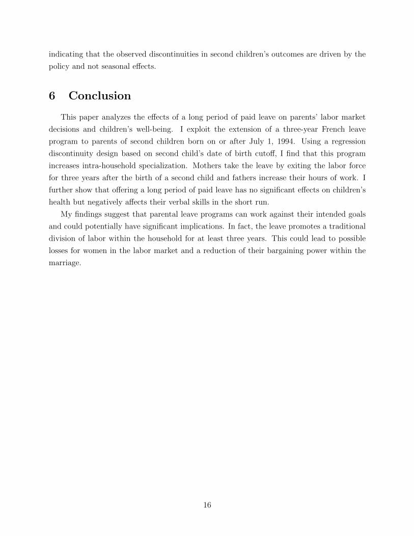
Effect of APE on Fathers’ Labor Market Outcomes

Both parents are eligible to receive APE benefits and some previous studies show that fathers

may be incentivized to take up parental leave (Bartel et al. 2015). To understand whether

12

fathers are induced to take the APE, I focus on their labor force participation and likelihood

of part-time work in Panels A and B of Figure 3 and columns 1 and 2 of Table 4. Both

graphs are smooth around the cutoff and the estimates are not statistically significant. This

indicates that fathers do not seem to benefit from the leave and is consistent with previous

reports which document that 98% of APE recipients are women.

Fathers can still however change their labor market behavior due to mothers’ take-up of

the leave. In fact, the APE does not provide full wage replacement, which could lead to a

decrease in household income and push men to try to compensate for that loss. Furthermore,

if couples substitute their time in home production, then fathers’ opportunity cost from

working might decrease which would induce them to work more.

In Panels C through E of Figure 3 and columns 3 to 5 of Table 4, I look at men’s labor

market behavior along the intensive margin. Men’s usual hours of work are not affected

by the APE extension but there is a clear discontinuity at the cutoff in actual hours of

work. This corresponds to an increase of around 2.6 hours per week. In Panel E, I find no

significant impact of the APE on father’s natural log of wages. Table A6 shows that the

regression estimates for fathers’ outcomes are robust to using different bandwidths as well

as to including controls and second child’s month of birth fixed effects.

The increase in actual work hours might be driven by either an increase in overtime hours

or a decrease in work absences. In Figure A6, I examine which channel is more likely to

drive the observed effects. Panel A plots overtime hours– i.e. the difference between actual

and usual hours of work for individuals with a regular work schedule– as a function of the

running variable. The graph does not exhibit any clear discontinuities and the estimates in

Table A7 are not statistically significant. Panel B shows that the probability that a father

works less than usual hours during the reference week decreases by 5.2 percentage points at

the cutoff. This is likely driven by a 4.4 percentage points decrease in the probability of not

working during the reference week (Panel D), while no significant effects are observed for

the likelihood of having a short workweek (Panel C).11 Taken together, these results suggest

that fathers are increasing their work hours through taking less time off from work.

Finally, the different panels in Figure A7 and Table A8 show the impact of the APE on

fathers’ main labor market outcomes in the first year after the birth of the second child.

Again, I find no effect on fathers’ likelihood of exiting the labor force or working part-time,

albeit the estimates are imprecise. I also find no significant effects on usual and actual hours

as well as the log of wages, suggesting that men adjust their work hours following mothers’

11Having an unworked week is defined as having 0 actual hours of work during the reference week forindividuals with both regular and irregular work schedules. Having a short workweek is the likelihood ofhaving positive actual hours during the reference week, that are lower than usual hours of work.

13

leave take-up.

Placebo Tests

I conduct two placebo tests to show that my results are indeed driven by the extension of the

APE. First, I examine whether we see significant effects in parents’ main outcomes using July

1992 as a fake cutoff. Panels A and B of Figure A8 plot mothers’ labor force participation

and fathers’ actual work hours as a function of the month-year of birth of the second child but

around the July 1992 threshold. Both graphs reveal no significant treatment effects. Table

A9 further shows regression discontinuity estimates for the main outcomes when shifting the

eligibility cutoff by 18 and 24 months on either side of the actual cutoff. Again, we see no

significant effects on any of these outcomes which implies that my results are driven by the

policy and not seasonal effects.

Second, I check for discontinuities in the main outcomes when using the month-year of

birth of the first child as a running variable in Panels C and D of Figure A8. Given that

parents of first children are not eligible for APE benefits, we should not see any discontinuities

at the threshold. The graphs for mothers’ labor force participation and fathers’ actual hours

of work are smooth at the cutoff and the regression estimates from this exercise, reported in

Table A10 are not significant for various outcomes of interest.

5.2 Children’s Outcomes

I now analyze the effects of the APE extension on children’s outcomes. I start by

discussing why parental leave is expected to affect children’s well-being. I then show results

for measures of children’s health and verbal development at age 6.

Parental leave and children’s outcomes

The main channel through which parental leave can affect a child’s health and development

is through increasing the time that parents spend at home. Mothers’ time away from work

is associated with an increase in the incidence and length of breastfeeding, as well as more

frequent medical check-ups and closer monitoring of children (Berger, Hill and Waldfogel,

2005; Baker and Milligan, 2008). Breastfeeding in particular can decrease the occurrence

of certain diseases and may have positive effects on children’s cognitive outcomes (Ruhm,

2000; Tanaka, 2005). While the evidence regarding paternal involvement is scarce, it is often

believed that increased time spent with the father can have positive effects on the child’s

development (El Nokali, Bachman and Votruba-Drzal, 2010).

An increase in parents’ time at home usually reduces the time that the child spends

14

with other caregivers. Although it is important for the child to bond with his mother in his

first year, he/she could benefit more from interacting with other individuals at a later age

(Dustmann and Schonberg, 2012).

A child’s well-being can also be affected by a loss of household income. Specifically,

negative income shocks can reduce access to health care, pediatric services and investments

in child-related goods and services. This might deteriorate the child’s health and impede

his development. The APE offers partial compensation to parents who wish to exit the

labor force or switch to part-time work. In that sense, it could lead to a loss of income for

some households. However, it is unlikely that this would reduce access to medical services

because France has a universal health care system.

Effect of APE on children’s health and verbal development

I now turn to the effects of the APE on children’s outcomes. I start by looking at how

APE eligibility affects various measures of child health. I first focus on measures that could

indicate closer monitoring of children. Specifically, Table 5 reports regression discontinuity

estimates for the number of Hepatitis B vaccines a child received by age 6, as well as dummy

variables for whether the child had the measles-mumps-rubella vaccine (MMR), whether the

child has an untreated cavity and whether the child is overweight. I find no significant effects

on any of these outcomes. Table 5 also shows results for whether a child has asthma or a

chronic disease, since breastfeeding is usually negatively correlated with the incidence of such

diseases. Again, the estimates are not statistically significant implying that the APE has no

impact on children’s health.

Next, I examine how the APE affects children’s verbal development at age 6. To do so,

Panels A and B of Figure 4 respectively plot dummy variables for whether the child has a

normal score on phonological awareness and vocabulary development tests. The figures show

a clear drop at the cutoff. Panel A of Table 6 indicates that children experience a 3.8 and

2.4 percentage points decrease in the likelihood of having normal scores on these tests.

As a placebo test, I check for discontinuities in these outcomes for first children and using

the month and year of birth of the first child as the running variable in Panels C and D of

Figure 4. The intuition here is that since parents of first children are not eligible to receive

the APE, we should not expect to see any discontinuities in these outcomes. Consistent with

ex-ante expectations, both graphs show no discontinuities at the cutoffs.

As an additional robustness check, I investigate whether my regression discontinuity

estimates are robust when using a difference-in-discontinuity approach with first children as

a control group. These estimates are presented in Panel B of Table 6. Although precision

is reduced, the estimates are close to the ones from the regression discontinuity approach,

15

indicating that the observed discontinuities in second children’s outcomes are driven by the

policy and not seasonal effects.

6 Conclusion

This paper analyzes the effects of a long period of paid leave on parents’ labor market

decisions and children’s well-being. I exploit the extension of a three-year French leave

program to parents of second children born on or after July 1, 1994. Using a regression

discontinuity design based on second child’s date of birth cutoff, I find that this program

increases intra-household specialization. Mothers take the leave by exiting the labor force

for three years after the birth of a second child and fathers increase their hours of work. I

further show that offering a long period of paid leave has no significant effects on children’s

health but negatively affects their verbal skills in the short run.

My findings suggest that parental leave programs can work against their intended goals

and could potentially have significant implications. In fact, the leave promotes a traditional

division of labor within the household for at least three years. This could lead to possible

losses for women in the labor market and a reduction of their bargaining power within the

marriage.

16

References

Almond, D., Currie, J., 2011. Human Capital Development before Age Five, in O. Ashenfleterand D. Card, eds., Handbook of Labor Economics, Vol. 4, Elsevier: 1315-1486.

Afsa, C., 1999. L’allocation parentale d’education : entre politique familiale et politique pourl’emploi. in INSEE, Donnees Sociales: La Societe Francaise. Paris: OECD.

Baker, M., Milligan, K., 2008. Maternal employment, breastfeeding, and health: Evidencefrom maternity leave mandates. Journal of Health Economics 27 (4): 871-887.

Baker, M., Milligan, K., 2010. Evidence from maternity leave expansions of the impact ofmaternal care on early child development. Journal of Human Resources 45 (1): 1-32.

Baker, M., Milligan, K., 2015. Maternity Leave and Children’s Cognitive and BehavioralDevelopment. Journal of Population Economics 28 (2): 373-391.

Bartel, A., Rossin-Slater, M., Ruhm, C.J., Stearns, J., Waldfogel, J., 2015. Paid FamilyLeave, Fathers’ Leave-Taking, and Leave-Sharing in Dual-Earner Households. UCSBWorking Paper.

Baum, C. L., 2003. The Effect of State Maternity Leave Legislation and the 1993 Familyand Medical Leave Act on Employment and Wages. Labour Economics 10 (5): 573- 596.

Berger, L.M., Hill, J., Waldfogel, J., 2005. Maternity leave, early maternal employment andchild health and development in the US. The Economic Journal 115: F29-F47.

Boyer, D., 2004. Les peres beneficiaires de l’APE: revelateurs de nouvelles pratiquespaternelles? Recherches et Previsions 76 (1): 53-62.

Calonico, S., Cattaneo, M.D., Titiunik, R., 2014. Robust Nonparametric Confidence Intervalsfor Regression-Discontinuity Designs. Econometrica 82 (6): 2295-2326.

Cameron, A.C., Gelbach, J.B., Miller, D.L., 2008. Bootstrap-based improvements forinference with clustered errors. The Review of Economics and Statistics 90 (3): 414-427.

Carneiro, P., Løken, K.V., Salvanes, K.G., 2015. A Flying Start? Maternity Leave Benefitsand Long Run Outcomes of Children. Journal of Political Economy 123 (2): 365-412.

Cools, S., Fiva, J.F., Kirkebøen, L., 2015. Causal Effects of Paternity Leave on Children andParents. The Scandinavian Journal of Economics 117 (3): 801-828.

Cullen, J.B., Gruber, J., 2000. Does unemployment insurance crowd out spousal laborsupply? Journal of Labor Economics 18 (3): 546-572.

Dahl, G.B., Løken, K.V., Mogstad, M., 2014. Peer Effects in Program Participation.American Economic Review 104 (7): 2049-2074.

17

Dahl, G.B., Løken, K.V., Mogstad, M., Salvanes, K.V., forthcoming. What is the Case forPaid Maternity Leave? The Review of Economics and Statistics.

Danzer, N., Lavy, V., 2014. Parental Leave and Children’s Schooling Outcomes: Quasi-Experimental Evidence from a Large Parental Leave Reform. University of WarwickWorking Paper.

Dustmann, C., Schonberg, U., 2012. Expansions in Maternity Leave Coverage and Children’sLong-Term Outcomes. American Economic Journal: Applied Economics 4 (3): 190-224.

Ekberg, J., Eriksson, R., Friebel, G., 2013. Parental Leave– A Policy Evaluation of theSwedish “Daddy-Month” Reform. Journal of Public Economics 97: 131-143.

El Nokali, N.E., Bachman, H.J., and Votruba-Drzal, E., 2010. Parent involvement andchildren’s academic and social development in elementary school. Child Development81 (3): 988-1005.

Flipo, A., Olier, L., 1996. Faire garder ses enfants: ce que les menages depensent. INSEEPremiere 481.

Gelber, A.M., 2014. Taxation and the earnings of husbands and wives: evidence from Sweden.The Review of Economics and Statistics 96 (2): 287-305.

Goux, D., Maurin, E., 2010. Public school availability for two-year olds and mothers’ laboursupply. Labour Economics 17 (6): 951-962.

Goux, D., Maurin, E., Petrongolo, B., 2014. Worktime regulations and spousal labor supply.American Economic Review 104 (1): 252-276.

Han, W.-J., Ruhm, C., Waldfogel, J., 2009. Parental Leave Policies and Parents’ Employmentand Leave-Taking. Journal of Policy Analysis and Management 28 (1): 29-54.

Imbens, G.W., Lemieux, T., 2008. Regression discontinuity designs: A guide to practice.Journal of Econometrics 142 (2): 615-635.

Kalil, A., Mogstad, M., Rege, M., Votruba, M.E., forthcoming. Father Presence and theIntergenerational Transmission of Educational Attainment. Journal of Human Resources.

Lalive, R., Schlosser, A., Steinhauer, A., Zweimuller, J., 2014. Parental Leave and Mothers’Careers: The Relative Importance of Job Protection and Cash Benefits. The Review ofEconomic Studies 81 (1): 219-265.

Lalive, R., Zweimuller, J., 2009. How Does Parental Leave Affect Fertility and Return toWork? Evidence from Two Natural Experiments. Quarterly Journal of Economics 124(3): 1363-1402.

Lee, D.S., Card, D., 2008. Regression discontinuity inference with specification error. Journalof Econometrics 142 (2): 655-674.

18

Lee, D.S., Lemieux, T., 2010. Regression discontinuity designs in economics. Journal ofEconomic Literature 48 (2): 281-355.

Lequien, L., 2012. The impact of parental leave duration on later wages. Annals of Economicsand Statistics 107-108: 267-285.

Liu, Q., Skans, O.N., 2010. The Duration of Paid Parental Leave and Children’s ScholasticPerformance. The B.E. Journal of Economic Analysis and Policy 10 (1): 1-35.

Ludsteck, J., Schonberg, U., 2014. Expansions in Maternity Leave Coverage and Mothers’Labor Market Outcomes after Childbirth. Journal of Labor Economics 32 (3): 469-505.

Lundberg, S., 1985. The added worker effect. Journal of Labor Economics 3 (1): 11-37.

Lundberg, S., 1988. Labor Supply of Husbands and Wives: A Simultaneous EquationsApproach. The Review of Economics and Statistics 70 (2): 224-235.

Lundberg, S., Rose, E., 1999. The Determinants of Specialization within Marriage. Universityof Washington mimeo.

Lundberg, S., Rose, E., 2000. Parenthood and the Earnings of Married Men and Women.Labour Economics 7 (6): 689-710.

Lundberg, S., Rose, E., 2002. The Effects of Sons and Daughters on Men’s Labor Supplyand Wages. The Review of Economics and Statistics 84 (2): 251-268.

Piketty, T., 2005. Impact de l’allocation parentale d’education sur l’activite feminine et lafecondite en France. Histoires de familles, histoires familiales 156: 79-109

Rasmussen, A.W., 2010. Increasing the Length of Parents’ Birth-Related Leave: The Effecton Children’s Long-Term Educational Outcomes. Labour Economics 17 (1): 91-100.

Rossin, M., 2011. The Effects of Maternity Leave on Children’s Birth and Infant HealthOutcomes in the United States. Journal of Health Economics 30 (2): 221-239.

Ruhm, C. J., 1998. The Economic Consequences of Parental Leave Mandates: Lessons fromEurope. The Quarterly Journal of Economics 113 (1): 285-317.

Ruhm, C. J., 2000. Parental leave and child health. Journal of Health Economics 19 (6):931-960.

Ruhm, C.J., 2011. Policies to Assist Parents with Young Children. The Future of Children21: 37-68.

Tanaka, S., 2005. Parental leave and child health across OECD countries. The EconomicJournal 115: F7-F28.

Tanaka, S., Waldfogel, J., 2007. Effects of Parental Leave and Working Hours on Fathers’Involvement with Their Babies: Evidence from the UK Millennium Cohort Study.Community, Work, and Family 10 (4): 407-424.

19

Waldfogel, J., 1999. The Impact of the Family and Medical Leave Act. Journal of PolicyAnalysis and Management 18 (2): 281-302.

20

Figure 1: Frequency of the running variable

21

Figure 2: Effect of APE on Mothers’ Labor Market Outcomes

(a) Probability of being out of the labor force (b) Probability of working part-time

(c) Natural log of wages (d) Probability of being employed

22

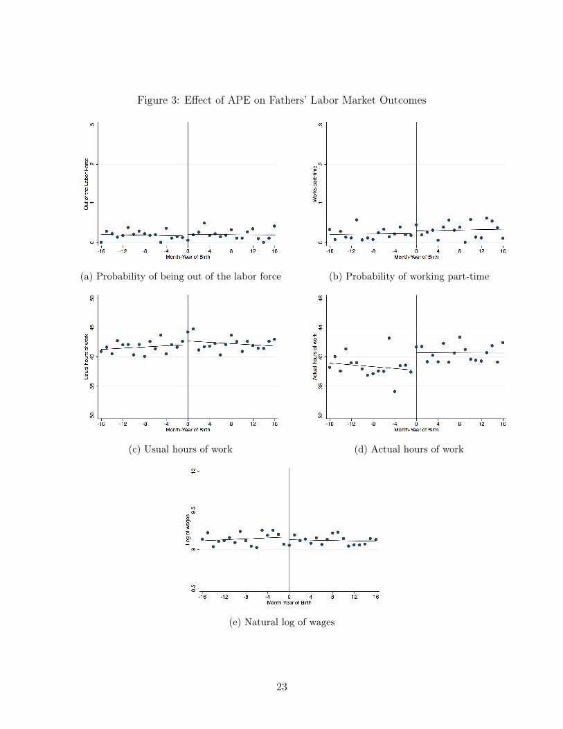
Figure 3: Effect of APE on Fathers’ Labor Market Outcomes


(c) Usual hours of work (d) Actual hours of work

(e) Natural log of wages

23

Figure 4: Effect of APE on Children’s Verbal Development

(a) Second child’s phonological awareness (b) Second child’s vocabulary development

(c) First child’s phonological awareness (d) First child’s vocabulary development

24

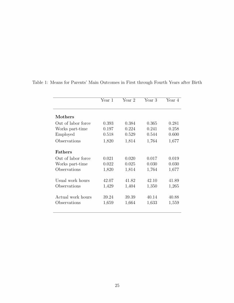
Table 1: Means for Parents’ Main Outcomes in First through Fourth Years after Birth

Year 1 Year 2 Year 3 Year 4

Mothers

Out of labor force 0.393 0.384 0.365 0.281Works part-time 0.197 0.224 0.241 0.258Employed 0.518 0.529 0.544 0.600

Observations 1,820 1,814 1,764 1,677

Fathers

Out of labor force 0.021 0.020 0.017 0.019Works part-time 0.022 0.025 0.030 0.030Observations 1,820 1,814 1,764 1,677

Usual work hours 42.07 41.82 42.10 41.89Observations 1,429 1,404 1,350 1,265

Actual work hours 39.24 39.39 40.14 40.88Observations 1,659 1,664 1,633 1,559

25

Table 2: Means for Children’s Main Outcomes

Mean Observations

Health Indicators

Number of Hepatitis B vaccines 1.259 7,610

Had MMR vaccine 0.937 7,610

Has untreated cavity 0.137 7,610

Is overweight 0.136 7,610

Has asthma 0.061 7,610

Has chronic disease 0.044 7,610

Tests of Verbal Skills

Phonological awareness is normal 0.879 6,197

Vocabulary development is normal 0.927 6,197

26

Table 3: Local Linear Regression Estimates for Mothers’ Labor Market Outcomes

Probability ofbeing out oflabor force

Probability ofworkingpart-time

Natural log ofwages

Probability ofbeingemployed

(1) (2) (3) (4)

Panel A:No Controls 0.167*** 0.002 – 0.019 – 0.137***

(0.025) (0.024) (0.062) (0.023)

Panel B:

With Controls 0.150*** 0.028 – 0.029 – 0.115***(0.025) (0.020) (0.037) (0.020)

Observations 5,255 5,255 2,638 5,255

Notes: Each cell reports the reduced form estimate of the effect of the APE on the corresponding outcome.Panel A shows estimates from regressions that do not include controls. Panel B reports coefficients fromregressions that account for second child’s month of birth fixed effects (except for the bandwidth of 4months), dummy variables for whether the second child is male, whether the second child is French,whether parents were born in France, parents’ age at the birth of the second child, and fixed effectsfor parents’ socioeconomic background and parents’ highest diploma. Standard errors are clusteredby month-year of birth of the second child and are reported in parentheses (*** p < 0.01 ** p <0.05 * p <0.1).

27

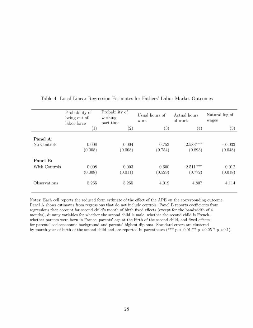
Table 4: Local Linear Regression Estimates for Fathers’ Labor Market Outcomes

Probability ofbeing out oflabor force

Probability ofworkingpart-time

Usual hours ofwork

Actual hoursof work

Natural log ofwages

(1) (2) (3) (4) (5)

Panel A:No Controls 0.008 0.004 0.753 2.583*** – 0.033

(0.008) (0.008) (0.754) (0.893) (0.048)

Panel B:

With Controls 0.008 0.003 0.600 2.511*** – 0.012(0.008) (0.011) (0.529) (0.772) (0.018)

Observations 5,255 5,255 4,019 4,807 4,114

Notes: Each cell reports the reduced form estimate of the effect of the APE on the corresponding outcome.Panel A shows estimates from regressions that do not include controls. Panel B reports coefficients fromregressions that account for second child’s month of birth fixed effects (except for the bandwidth of 4months), dummy variables for whether the second child is male, whether the second child is French,whether parents were born in France, parents’ age at the birth of the second child, and fixed effectsfor parents’ socioeconomic background and parents’ highest diploma. Standard errors are clusteredby month-year of birth of the second child and are reported in parentheses (*** p < 0.01 ** p <0.05 * p <0.1).

28

Table 5: Regression Estimates for Indicators of Child Health

HB vaccines MMR vaccine Untreated Cavity Is Overweight Has Asthma Chronic Disease(1) (2) (3) (4) (5) (6)

RD Estimate -0.051 -0.007 0.017 0.015 0.008 -0.004[0.468] [0.554] [0.280] [0.315] [0.410] [0.677]

Observations 7,610 7,610 7,610 7,610 7,610 7,610

*** p <0.01 ** p <0.05 * p <0.1.This table shows regression discontinuity estimates for various indicators of child health.The numbers in brackets are p-values computed using a clustered wild bootstrap-t procedure.

29

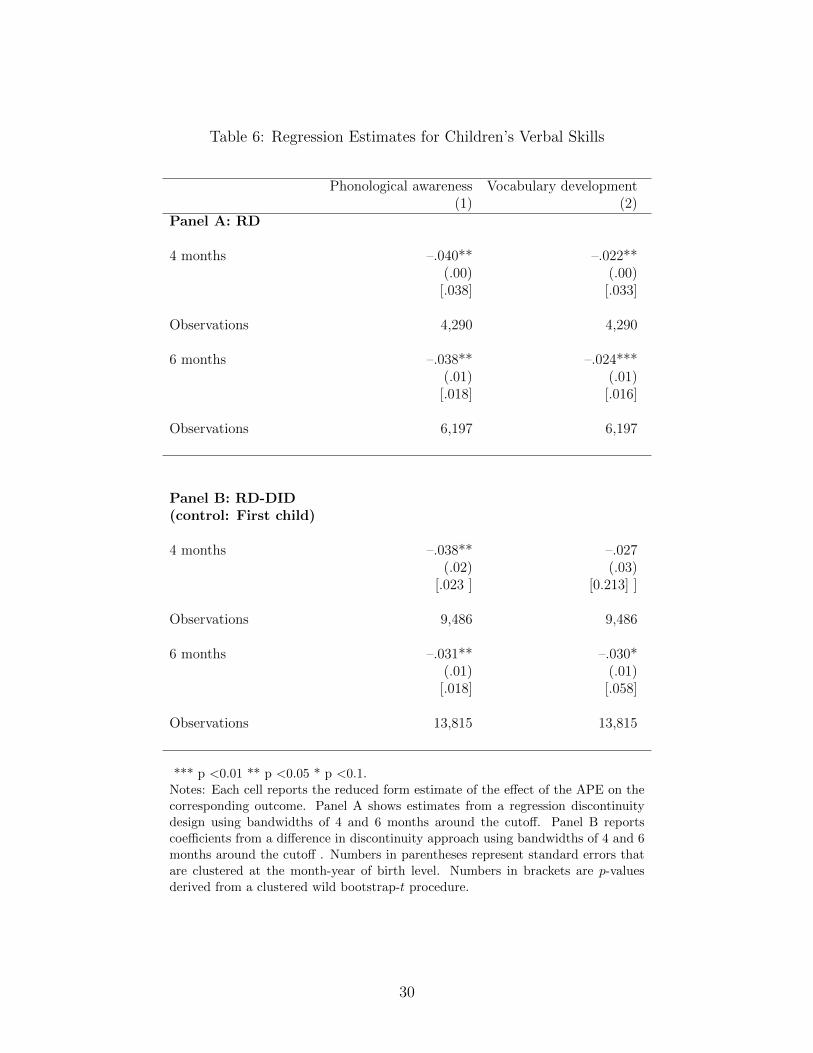
Table 6: Regression Estimates for Children’s Verbal Skills

Phonological awareness Vocabulary development(1) (2)

Panel A: RD

4 months –.040** –.022**(.00) (.00)

[.038] [.033]

Observations 4,290 4,290

6 months –.038** –.024***(.01) (.01)

[.018] [.016]


Panel B: RD-DID(control: First child)

4 months –.038** –.027(.02) (.03)

[.023 ] [0.213] ]


6 months –.031** –.030*(.01) (.01)

[.018] [.058]


*** p <0.01 ** p <0.05 * p <0.1.Notes: Each cell reports the reduced form estimate of the effect of the APE on thecorresponding outcome. Panel A shows estimates from a regression discontinuitydesign using bandwidths of 4 and 6 months around the cutoff. Panel B reportscoefficients from a difference in discontinuity approach using bandwidths of 4 and 6months around the cutoff . Numbers in parentheses represent standard errors thatare clustered at the month-year of birth level. Numbers in brackets are p-valuesderived from a clustered wild bootstrap-t procedure.

30

A Appendix Figures and Tables

Figure A1: Smoothness of Baseline Covariates

(a) Second child is male (b) Mother’s age at second child’s birth

(c) Father’s age at second child’s birth (d) Mother born in France

(e) Father born in France

31

Figure A2: Parents’ Educational Level

(a) Mother has no diploma (b) Father has no diploma

(c) Mother has high school degree (d) Father has high school degree

(e) Mother has college degree (f) Father has college degree

32

Figure A3: Parents’ Socioeconomic Background

(a) Mother’s father is manual worker (b) Father’s father is manual worker

(c) Mother’s father in high-skilled occupation (d) Father’s father in high-skilled occupation

(e) Mother’s father in other occupations (f) Father’s father in other occupations

33

Figure A4: Additional Results for Mothers’ Labor Market Outcomes in Second throughFourth Years After Birth

(a) Probability of being a stay-at-home mother(b) Probability of working in intermediate occu-pation

(c) Probability of being in managerial or high-level occupation

(d) Probability of being in liberal profession or anentrepreneur

(e) Probability of being a manual worker

34

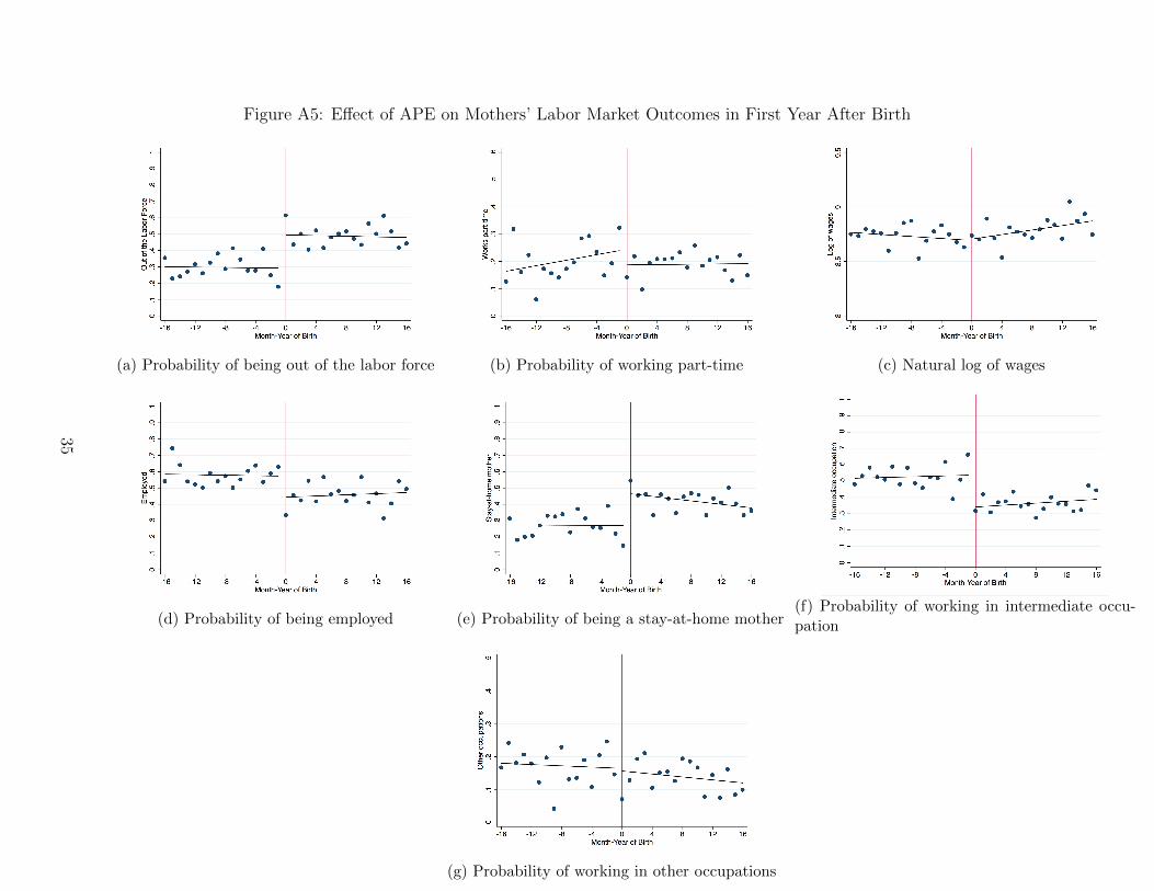
Figure A5: Effect of APE on Mothers’ Labor Market Outcomes in First Year After Birth

(a) Probability of being out of the labor force (b) Probability of working part-time (c) Natural log of wages

(d) Probability of being employed (e) Probability of being a stay-at-home mother(f) Probability of working in intermediate occu-pation

(g) Probability of working in other occupations

35

Figure A6: Additional Results for Fathers’ Labor Market Outcomes in Second throughFourth Years After Birth

(a) Overtime hours (b) Works less than usual hours

(c) Probability of short workweek (d) Probability of unworked week

36

Figure A7: Effect of APE on Fathers’ Labor Market Outcomes in First Year After Birth


(c) Usual hours of work (d) Actual hours of work

(e) Natural log of wages

37

Figure A8: Placebo Tests

Cutoff is July 1992

(a) Mothers out of the labor force (b) Fathers’ actual hours of work

Running variable is month-year of birth of first child

(c) Mothers out of the labor force (d) Fathers’ actual hours of work

38

Table A1: Regression Estimates for Baseline Covariates Using Different Bandwidths

Bandwidth 4 months 13 months 16 months 19 months 22 months 28 months(1) (2) (3) (4) (5) (6)

Second child is male – 0.025 – 0.021 – 0.010 – 0.018 – 0.020 – 0.025(0.020) (0.025) (0.025) (0.022) (0.021) (.026)

Mother’s age 0.281 0.220 0.130 0.054 0.078 0.131(0.293) (0.288) (0.288) (0.263) (0.245) (0.299)

Father’s age 0.017 0.188 0.006 0.002 0.038 0.092(0.245) (0.249) (0.245) (0.219) (0.218) (0.253)

Mother born in France 0.008 0.020 0.013 0.011 0.013 0.024(0.023) (0.024) (0.022) (0.020) (0.018) (0.024)

Father born in France – 0.014 – 0.020 – 0.010 – 0.014 – 0.009 – 0.027(0.020) (0.019) (0.019) (0.017) (0.017) (0.020)

Mother no diploma 0.017 0.019 –0.007 –0.001 –0.008 0.030(0.022) (0.031) (0.030) (0.026) (0.024) (0.031)

Father no diploma 0.010 0.003 –0.005 0.009 0.024 0.027(0.019) (0.023) (0.021) (0.019) (0.020) (0.028)

Mother high school 0.030 0.044 – 0.008 0.028 0.025 0.040(0.022) (0.027) (0.026) (0.028) (0.028) (0.026)

Father high school 0.009 0.011 0.011 0.021 0.009 0.003(0.026) (0.028) (0.029) (0.026) (0.025) (0.030)

Mother college – 0.029 – 0.030 – 0.014 – 0.013 – 0.013 – 0.029(0.027) (0.030) (0.027) (0.024) (0.022) (0.030)

Father college – 0.012 0.000 0.010 0.001 – 0.003 – 0.002(0.021) (0.023) (0.022) (0.019) (0.017) (0.024)

Polynomial Zero One One One One TwoObservations 1011 3202 3990 4738 5481 7010

Notes: Each cell reports the reduced form estimate of the effect of the APE on a baseline covariate,using bandwidths that are within 3, 6 and 12 months from the preferred bandwidth (i.e. 16 months).For the variable “Mother has a high school degree”, estimates for bandwidths ≥ 16 months are takenfrom regressions with a polynomial of degree 2 in the running variable. Standard errors are clustered bymonth-year of birth of the second child and are reported in parentheses. (*** p < 0.01 ** p <0.05 * p <0.1).

39

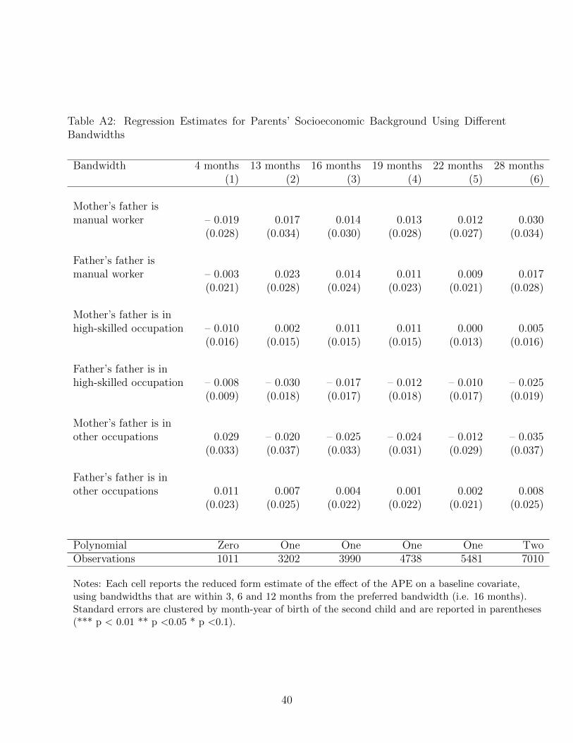
Table A2: Regression Estimates for Parents’ Socioeconomic Background Using DifferentBandwidths


Mother’s father ismanual worker – 0.019 0.017 0.014 0.013 0.012 0.030

(0.028) (0.034) (0.030) (0.028) (0.027) (0.034)

Father’s father ismanual worker – 0.003 0.023 0.014 0.011 0.009 0.017

(0.021) (0.028) (0.024) (0.023) (0.021) (0.028)

Mother’s father is inhigh-skilled occupation – 0.010 0.002 0.011 0.011 0.000 0.005

(0.016) (0.015) (0.015) (0.015) (0.013) (0.016)

Father’s father is inhigh-skilled occupation – 0.008 – 0.030 – 0.017 – 0.012 – 0.010 – 0.025

(0.009) (0.018) (0.017) (0.018) (0.017) (0.019)

Mother’s father is inother occupations 0.029 – 0.020 – 0.025 – 0.024 – 0.012 – 0.035

(0.033) (0.037) (0.033) (0.031) (0.029) (0.037)

Father’s father is inother occupations 0.011 0.007 0.004 0.001 0.002 0.008

(0.023) (0.025) (0.022) (0.022) (0.021) (0.025)

Polynomial Zero One One One One TwoObservations 1011 3202 3990 4738 5481 7010

Notes: Each cell reports the reduced form estimate of the effect of the APE on a baseline covariate,using bandwidths that are within 3, 6 and 12 months from the preferred bandwidth (i.e. 16 months).Standard errors are clustered by month-year of birth of the second child and are reported in parentheses(*** p < 0.01 ** p <0.05 * p <0.1).

40

Table A3: Regression Estimates for Mothers’ Labor Market Outcomes in Second throughFourth Years after Birth Using Different Bandwidths


Panel A:Out of the labor force

No controls 0.194*** 0.200*** 0.167*** 0.140*** 0.139*** 0.176***(0.022) (0.022) (0.025) (0.026) (0.025) (0.028)

With controls 0.190*** 0.205*** 0.150*** 0.126*** 0.121*** 0.145***(0.020) (0.020) (0.025) (0.023) (0.023) (0.035)

Panel B:Works part-time

No controls – 0.038** – 0.026 0.002 0.004 – 0.002 0.002(0.014) (0.022) (0.024) (0.020) (0.019) (0.024)

With controls – 0.033** 0.017 0.028 0.027 0.031* 0.027(0.013) (0.029) (0.020) (0.019) (0.018) (0.028)

Panel C:Natural log of wages

No controls 0.005 0.026 – 0.019 – 0.022 – 0.024 – 0.021(0.070) (0.067) (0.062) (0.055) (0.050) (0.069)

With controls – 0.009 0.053 – 0.029 – 0.024 – 0.025 – 0.018(0.044) (0.040) (0.037) (0.035) (0.033) (0.043)

Panel D:Employed

No controls – 0.159*** – 0.162*** – 0.137*** – 0.118*** – 0.128*** – 0.138***(0.019) (0.025) (0.023) (0.022) (0.021) (0.027)

With controls – 0.155*** – 0.139*** – 0.115*** – 0.101*** – 0.101*** – 0.102***(0.015) (0.018) (0.020) (0.020) (0.020) (0.028)

Polynomial Zero One One One One Two

Obs. (Panels A,B,D) 1,339 4,224 5,255 6,254 7,239 9,264Obs. (Panel C) 655 2,112 2,638 3,177 3,677 4,717

Notes: Each cell reports the reduced form estimate of the effect of the APE on the corresponding outcome,using bandwidths that are within 3, 6 and 12 months from the preferred bandwidth (i.e. 16 months).Results are shown both with and without controls. Controls include second child’s month of birth fixedeffects (except for the bandwidth of 4 months), dummy variables for whether the second child is male,whether the second child is French, whether parents were born in France, parents’ age at the birth ofthe second child, and fixed effects for parents’ socioeconomic background and parents’ highest diploma.Standard errors are clustered by month-year of birth of the second child and are reported in parentheses(*** p < 0.01 ** p <0.05 * p <0.1).

41

Table A4: Additional Results for Mothers’ Labor Market Outcomes in Second throughFourth Years after Birth


Panel A:Stay-at-home mother

No controls 0.185*** 0.185*** 0.156*** 0.137*** 0.135*** 0.168***(0.020) (0.022) (0.024) (0.025) (0.024) (0.027)

With controls 0.180*** 0.169*** 0.135*** 0.122*** 0.116*** 0.143***(0.024) (0.023) (0.023) (0.022) (0.022) (0.035)

Panel B:Intermediate occupationNo controls – 0.185*** – 0.182*** – 0.174*** – 0.149*** – 0.152*** – 0.174***

(0.025) (0.030) (0.030) (0.028) (0.027) (0.032)

With controls – 0.188*** – 0.188*** – 0.174*** – 0.150*** – 0.143*** – 0.159***(0.021) (0.028) (0.030) (0.029) (0.029) (0.036)

Panel C:Managerialor high-level occupation

No controls – 0.010 – 0.002 0.001 0.004 – 0.006 0.001(0.034) (0.033) (0.029) (0.027) (0.025) (0.034)

With controls 0.005 0.008 0.006 0.009 0.003 0.018(0.022) (0.011) (0.013) (0.011) (0.010) (0.016)

Panel D:Liberal professionor entrepreneur

No controls 0.014 0.006 0.008 0.012 0.012 0.007(0.008) (0.009) (0.009) (0.009) (0.008) (0.009)

With controls 0.010 0.003 0.012* 0.014** 0.012* 0.003(0.008) (0.005) (0.006) (0.006) (0.007) (0.008)

Panel E:Manual worker

No controls – 0.022 – 0.034 – 0.013 – 0.019 – 0.007 – 0.007(0.024) (0.023) (0.022) (0.019) (0.018) (0.025)

With controls – 0.017 – 0.033 0.004 – 0.001 0.004 – 0.007(0.024) (0.023) (0.018) (0.018) (0.015) (0.023)

Polynomial Zero One One One One TwoObservations 1,339 4,224 5,255 6,254 7,239 9,264

Notes: Each cell reports the reduced form estimate of the effect of the APE on the corresponding outcome,using bandwidths that are within 3, 6 and 12 months from the preferred bandwidth (i.e. 16 months).Results are shown both with and without controls. Controls include second child’s month of birth fixedeffects (except for the bandwidth of 4 months), dummy variables for whether the second child is male,whether the second child is French, whether parents were born in France, parents’ age at the birth of the secondchild, and fixed effects for parents’ socioeconomic background and parents’ highest diploma. Standard errorsare clustered by month-year of birth of the second child and are reported in parentheses (*** p < 0.01 ** p <0.05* p <0.1).

42

Table A5: Regression Estimates for Mothers’ Labor Market Outcomes in First Year afterBirth



No controls 0.218*** 0.216*** 0.199*** 0.204*** 0.218*** 0.228***(0.062) (0.063) (0.057) (0.050) (0.043) (0.063)

With controls 0.203** 0.214*** 0.150*** 0.169*** 0.184*** 0.190***(0.067) (0.052) (0.044) (0.040) (0.038) (0.068)


No controls – 0.062 – 0.104** – 0.064 – 0.050 – 0.046 – 0.083(0.043) (0.046) (0.043) (0.038) (0.035) (0.047)

With controls – 0.049 – 0.084** – 0.024 – 0.013 – 0.000 – 0.045(0.049) (0.034) (0.034) (0.030) (0.030) (0.045)

Panel C:Natural log of wages

No controls 0.042 0.034 – 0.007 0.019 0.040 0.019(0.055) (0.058) (0.054) (0.052) (0.053) (0.062)

With controls 0.046 0.074 0.025 0.003 0.020 0.019(0.056) (0.056) (0.050) (0.049) (0.050) (0.068)

Panel D:Employed

No controls – 0.159** – 0.177*** – 0.126** – 0.118*** – 0.134*** – 0.138***(0.046) (0.042) (0.047) (0.040) (0.035) (0.049)

With controls – 0.146** – 0.177*** – 0.069* – 0.077** – 0.090*** – 0.081(0.049) (0.036) (0.040) (0.036) (0.033) (0.057)

Panel E:Stay-at-home-mother

No controls 0.202** 0.213*** 0.191*** 0.183*** 0.185*** 0.219***(0.062) (0.059) (0.055) (0.051) (0.044) (0.061)

With controls 0.193** 0.184*** 0.131*** 0.137*** 0.146*** 0.189***(0.071) (0.048) (0.040) (0.039) (0.036) (0.064)

Panel F:Intermediate Occupation

No controls – 0.189** – 0.182*** – 0.189*** – 0.190*** – 0.210*** – 0.209***(0.059) (0.058) (0.053) (0.047) (0.043) (0.063)

With controls – 0.188** – 0.218*** – 0.172*** – 0.176*** – 0.202*** – 0.204***(0.055) (0.037) (0.040) (0.035) (0.035) (0.063)

Panel G:Other Occupation

No controls – 0.033 – 0.038 – 0.011 – 0.016 – 0.013 – 0.019(0.042) (0.041) (0.039) (0.035) (0.032) (0.045)

With controls – 0.024 0.003 0.020 0.006 0.014 0.015(0.044) (0.037) (0.032) (0.030) (0.027) (0.038)

Polynomial Zero One One One One OneObs. (Panels A,B,D, E, F, G) 457 1,468 1,820 2,159 2,464 3,119Obs. (Panel C) 212 678 856 1,031 1,169 1,464

Notes: Each cell reports the reduced form estimate of the effect of the APE on the corresponding outcome, usingbandwidths that are within 3, 6 and 12 months from the preferred bandwidth (i.e. 16 months). Results are shownboth with and without controls. Controls include second child’s month of birth fixed effects (except for thebandwidth of 4 months), dummy variables for whether the second child is male, whether the second child is French,whether parents were born in France, parents’ age at the birth of the second child, and fixed effects for parents’socioeconomic background and parents’ highest diploma. Standard errors are clustered by month-year of birth of thesecond child and are reported in parentheses (*** p < 0.01 ** p <0.05 * p <0.1).

43

Table A6: Regression Estimates for Fathers’ Labor Market Outcomes in Second throughFourth Years after Birth Using Different Bandwidths



No controls 0.007 0.007 0.008 0.004 0.004 0.009(0.010) (0.008) (0.008) (0.007) (0.007) (0.009)

With controls 0.008 –0.009 0.008 0.003 0.002 0.003(0.010) (0.006) (0.008) (0.007) (0.007) (0.010)

Observations 1,339 4,224 5,255 6,254 7,239 9,264


No controls 0.006 0.009 0.004 0.013 0.011 0.011(0.007) (0.009) (0.008) (0.009) (0.008) (0.009)

With controls 0.006 0.023** 0.003 0.008 0.007 0.007(0.008) (0.011) (0.011) (0.010) (0.010) (0.013)

Observations 1,339 4,224 5,255 6,254 7,239 9,264

Panel C:Usual hours of work

No controls 1.261 1.095 0.753 1.127 1.561** 1.475*(0.881) (0.819) (0.754) (0.747) (0.684) (0.825)

With controls 1.437 0.991** 0.600 0.954* 1.428** 0.849(0.930) (0.423) (0.529) (0.559) (0.596) (0.766)

Observations 1,024 3,238 4,019 4,764 5,518 7,101

Panel D:Actual hours of work

No controls 2.693** 2.872*** 2.583*** 2.678*** 2.916*** 2.942***(0.820) (0.946) (0.893) (0.867) (0.803) (0.975)

With controls 2.483*** 3.741*** 2.511*** 2.405*** 2.709*** 2.772***(0.638) (0.806) (0.772) (0.811) (0.757) (0.973)

Observations 1,213 3,857 4,807 5,716 6,615 8,480

Panel E:Natural log of wages

No controls – 0.055 – 0.049 – 0.033 – 0.044 – 0.049 – 0.059(0.042) (0.052) (0.048) (0.043) (0.040) (0.055)

With controls – 0.019 – 0.016 – 0.012 – 0.014 – 0.009 – 0.018(0.022) (0.017) (0.018) (0.020) (0.019) (0.027)

Observations 1,032 3,305 4,114 4,869 5,668 7,276

Polynomial Zero One One One One Two


44

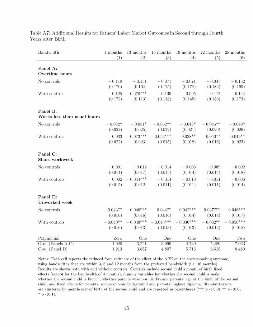
Table A7: Additional Results for Fathers’ Labor Market Outcomes in Second through FourthYears after Birth


Panel A:Overtime hours

No controls – 0.119 – 0.151 – 0.071 – 0.071 – 0.047 – 0.182(0.170) (0.164) (0.175) (0.178) (0.182) (0.199)

With controls – 0.125 – 0.370*** – 0.139 – 0.095 – 0.112 – 0.144(0.172) (0.113) (0.138) (0.145) (0.150) (0.173)

Panel B:Works less than usual hours

No controls – 0.042* – 0.051* – 0.052** – 0.043* – 0.045** – 0.049*(0.022) (0.025) (0.022) (0.021) (0.020) (0.026)

With controls – 0.033 – 0.073*** – 0.053*** – 0.038** – 0.040** – 0.049**(0.022) (0.023) (0.015) (0.018) (0.016) (0.023)

Panel C:Short workweek

No controls – 0.001 – 0.012 – 0.014 – 0.006 – 0.009 – 0.002(0.014) (0.017) (0.015) (0.014) (0.014) (0.018)

With controls 0.002 – 0.044*** – 0.014 – 0.010 – 0.014 – 0.006(0.015) (0.012) (0.011) (0.011) (0.011) (0.014)

Panel D:Unworked week

No controls – 0.043** – 0.046*** – 0.044** – 0.042*** – 0.037*** – 0.048***(0.016) (0.016) (0.016) (0.014) (0.014) (0.017)

With controls – 0.040** – 0.048*** – 0.045*** – 0.036*** – 0.032** – 0.050***(0.016) (0.013) (0.013) (0.013) (0.012) (0.018)

Polynomial Zero One One One One TwoObs. (Panels A-C) 1,020 3,221 3,999 4,739 5,489 7,063Obs. (Panel D) 1,213 3,857 4,807 5,716 6,615 8,480


45

Table A8: Regression Estimates for Fathers’ Labor Market Outcomes in First Year afterBirth



No controls 0.019 0.014 0.013 0.009 0.006 0.016(0.015) (0.015) (0.014) (0.013) (0.012) (0.016)

With controls 0.026 0.008 0.010 0.005 0.005 0.016(0.016) (0.014) (0.012) (0.012) (0.012) (0.014)

Observations 457 1,468 1,820 2,159 2,464 3,119


No controls 0.010 0.020 0.013 0.021* 0.013 0.026*(0.013) (0.013) (0.012) (0.011) (0.011) (0.013)

With controls 0.013 0.025** 0.014 0.025** 0.017 0.024*(0.014) (0.011) (0.010) (0.010) (0.010) (0.013)

Observations 457 1,468 1,820 2,159 2,464 3,119

Panel C:Usual hours of work

No controls – 1.017** – 1.407 – 1.211* – 1.396 – 0.582 – 1.525(0.418) (0.848) (0.702) (0.857) (0.842) (0.927)

With controls – 1.155* 0.542 2.251 – 0.038 2.370 – 0.729(.525) (.979) (1.446) (1.135) (1.635) (1.231)

Observations 357 1,164 1,429 1,696 1,927 2,433

Panel D:Actual hours of work

No controls – 1.553 – 1.327 – 0.425 – 0.591 – 0.117 – 0.819(1.414) (1.735) (1.964) (1.856) (2.228) (2.011)

With controls – 1.785* – 0.813 1.181 0.731 0.268 – 1.427(.895) (1.125) (1.963) (1.361) (2.223) (1.773)

Observations 421 1,341 1,659 1,968 2,241 2,854

Panel E:Natural log of wages

No controls – 0.022 – 0.039 – 0.044 – 0.050 – 0.042 – 0.074(0.044) (0.048) (0.041) (0.038) (0.035) (0.052)

With controls 0.001 0.027 – 0.022 – 0.040* – 0.025 – 0.034(0.018) (0.031) (0.022) (0.020) (0.022) (0.027)

Observations 372 1,156 1,426 1,695 1,931 2,463

Polynomial (Panels A,B,E) Zero One One One One TwoPolynomial (Panels C,D) Zero One Two Two Three Three


46

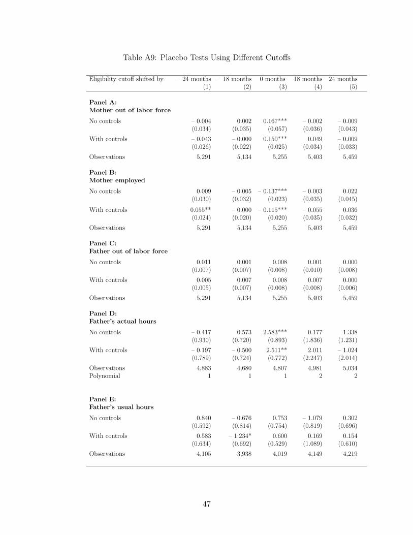
Table A9: Placebo Tests Using Different Cutoffs

Eligibility cutoff shifted by – 24 months – 18 months 0 months 18 months 24 months(1) (2) (3) (4) (5)

Panel A:Mother out of labor force

No controls – 0.004 0.002 0.167*** – 0.002 – 0.009(0.034) (0.035) (0.057) (0.036) (0.043)

With controls – 0.043 – 0.000 0.150*** 0.049 – 0.009(0.026) (0.022) (0.025) (0.034) (0.033)

Observations 5,291 5,134 5,255 5,403 5,459

Panel B:Mother employed

No controls 0.009 – 0.005 – 0.137*** – 0.003 0.022(0.030) (0.032) (0.023) (0.035) (0.045)

With controls 0.055** – 0.000 – 0.115*** – 0.055 0.036(0.024) (0.020) (0.020) (0.035) (0.032)

Observations 5,291 5,134 5,255 5,403 5,459

Panel C:Father out of labor force

No controls 0.011 0.001 0.008 0.001 0.000(0.007) (0.007) (0.008) (0.010) (0.008)

With controls 0.005 0.007 0.008 0.007 0.000(0.005) (0.007) (0.008) (0.008) (0.006)

Observations 5,291 5,134 5,255 5,403 5,459

Panel D:Father’s actual hours

No controls – 0.417 0.573 2.583*** 0.177 1.338(0.930) (0.720) (0.893) (1.836) (1.231)

With controls – 0.197 – 0.500 2.511** 2.011 – 1.024(0.789) (0.724) (0.772) (2.247) (2.014)

Observations 4,883 4,680 4,807 4,981 5,034Polynomial 1 1 1 2 2

Panel E:Father’s usual hours

No controls 0.840 – 0.676 0.753 – 1.079 0.302(0.592) (0.814) (0.754) (0.819) (0.696)

With controls 0.583 – 1.234* 0.600 0.169 0.154(0.634) (0.692) (0.529) (1.089) (0.610)

Observations 4,105 3,938 4,019 4,149 4,219

47

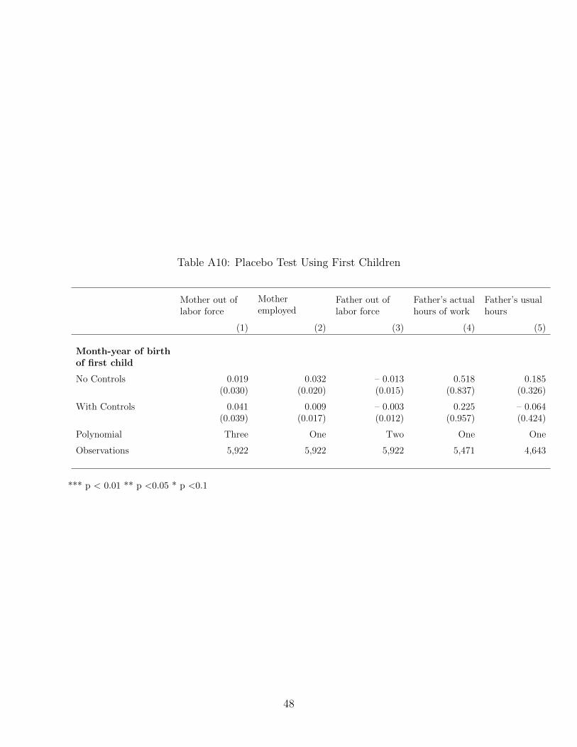
Table A10: Placebo Test Using First Children

Mother out oflabor force

Motheremployed

Father out oflabor force

Father’s actualhours of work

Father’s usualhours

(1) (2) (3) (4) (5)

Month-year of birthof first child

No Controls 0.019 0.032 – 0.013 0.518 0.185(0.030) (0.020) (0.015) (0.837) (0.326)

With Controls 0.041 0.009 – 0.003 0.225 – 0.064(0.039) (0.017) (0.012) (0.957) (0.424)

Polynomial Three One Two One One

Observations 5,922 5,922 5,922 5,471 4,643

*** p < 0.01 ** p <0.05 * p <0.1

48

parental leave, intra-household specialization and...

Documents