parental background, secondary school track choice, and - ucl

# Oxford University Press 2004 Oxford Economic Papers 56 (2004), 209–230 209All rights reserved DOI: 10.1093/oep/gpf048

Parental background, secondary schooltrack choice, and wages

By Christian Dustmann

Department of Economics, University College London, London WC1E 6BT;

e-mail: [email protected]

The way parents take influence on the education of their children is a crucial aspect

of intergenerational mobility. Unlike in the UK or in the US, in Germany an important

decision about which educational track to follow is made at a relatively early stage:

after primary school, at the age of ten. In this paper, we use micro data to analyse

the association between parents’ education and profession, and secondary track school

choice and subsequent career prospects of the child. Our analysis covers the last six

decades. We demonstrate that parental background is strongly related to the secondary

track choice of the child, and subsequent educational achievements. We find a slight

convergence for individuals from different parental background over the last decades.

We also find a positive trend for females to follow higher secondary school tracks,

keeping parental background constant. The association between parental class and

educational choice translates into substantial earnings differentials later in life.

1. IntroductionThe degree to which poverty, or wealth is transmitted from one generation to the

next is a key research area in social sciences. In economics, one growing strand

of research investigates intergenerational mobility of income status, trying to

establish the correlation between parents’ and childrens’ position in the income

distribution.1 This research, although carefully addressing identification problems

of earlier studies, does little to explain the mechanisms that underly intergenera-

tional income mobility.

In this paper, we investigate a particular aspect of intergenerational transmission.

We argue that one of the crucial factors for intergenerational mobility is the way

educational institutions allow parents to influence the education of their children.

Education is a process that proceeds in stages, and early educational career

decisions have a strong effect on the choices available at later stages. At what age

these decisions are taken, and how heavily they affect future opportunities, varies

between countries, and may be a key factor in explaining across-country variations

in intergenerational mobility.

..........................................................................................................................................................................1 See recent studies by Zimmerman, 1992, and Solon, 1992, for the US; Dearden et al., 1997, for the UK;

Bjoerklund and Jaenti, 1997, for Sweden; and Wiegand, 1999, for Germany. Solon, 1999, provides a

comprehensive overview of this literature.

Traditional models on investment in human capital (for instance, Ben Porath,

1967) work on the assumption that education is primarily a matter of individual

choice. This may be the case at later stages of the individual’s educational

career. However, early educational decisions are likely to be heavily affected

by parental background. A recent literature provides strong empirical evidence

for a link between overall educational achievements and parental background

(see, for instance, Feinstein and Symons, 1999, and Ermisch and Francesconi,

2001, for the UK).

A most important stage in this process is the choice of schools that qualify pupils

for different post-secondary education tracks, like university education. In Britain,

the choice for continued schooling that qualifies pupils for university or other

academic education is generally taken at the age of 16. In the US, high school

attendance that qualifies for college education is almost compulsory—according

to the Bureau of Labour Statistics, about 85% of a cohort finish high school success-

fully. Germany has a three-track system of secondary education. In 1990, only 27%

of school graduates graduated from the highest secondary track schools. It is only the

highest track (corresponding to high school in the US, or A-levels in the UK) that

allows for direct access to the university system. The decision about which track to

follow is made at a relatively early stage: after primary school, at about the age of ten.

Most research in economics does not address the secondary school track

decision, but starts with transitions after secondary school education.2 In this

paper, we investigate the way the choice of secondary school is related to parental

characteristics, and to future wages.3 Our analysis is for Germany, where the

decision about a particular educational track coincides with the primary–secondary

school transition.4

Germany has a standardised secondary education system, where all primary and

secondary schools are state schools. Schools at all levels (including universities) have

offered (since the 1950s) tuition free education. Ability tests which provide some

indication about the child’s potential (and which are common in the UK and

in the US) do not exist (any more) in Germany. There are recommendations

by the primary school teacher about which secondary track to choose, but these

recommendations are not binding. These features of the German education system,

210 parental background, choice, and wages

..........................................................................................................................................................................2 See Riphan, 1999, Merz and Schimmelpfennig, 1998; Couch, 1994, provides comparisons of transition

patterns between the US and Germany; Ryan, 2001, provides an excellent cross-national analysis.

Winkelmann, 1996a,b, Steedman, 1993, and Buechtemann et al., 1993, discuss the apprenticeship train-

ing scheme and subsequent transitions into the labour market.3 There are some studies that investigate income effects on educational pathways for Germany. Buechel

et al., 2000, find a strong association between income and the tendency to attend higher track. Jenkins

and Schlueter, 2002, examine income effects on childrens’ choice of secondary school tracks in more

detail.4 Investigation of primary–secondary school transitions has a history among educationalists. This litera-

ture focus primarily on the disruptions of transfers and transitions for pupils, affecting pupils’ attitudes,

motivation, and academic performance (see e.g. Galton et al., 1999, for the UK, and Caterall, 1998,

for the US).

and in particular the state provided financing, contribute to the view still held by

some that the system provides equal opportunities of educational choice.

We demonstrate in this paper that educational mobility is nevertheless limited.

We argue that one reason is the early choice of the secondary school education

track, which is heavily affected by the advice and the influence of the parents,

leading to intergenerational immobility in educational achievements. We demon-

strate further that the secondary school track the child follows is strongly correlated

with post-school educational choices, and that parental background, by way of

association with secondary track schools, has a most significant association with

the wage career of the individual.

This particular feature of the German education system—a strong institutional

differentiation instead of a comprehensive education at secondary level—had

been hold partly responsible for the low mean and the high variance of 15 years

old practical literacy scores in the PISA 2000 study, an assessment of knowledge

and skills of 15-year-olds in the principal industrialised countries (OECD,

2000). We argue that it may also lead to low educational mobility. Results of our

analysis are complementary to work by Shavit and Mueller (1998), who conclude

that early streaming of lower secondary school students in Germany creates a

particularly strong association between educational attainment and labour market

inequality.

We commence by analysing the association of parental education and profession

with the choice of secondary school education of the child over the last six decades.

We demonstrate that this association is very strong. There is a tendency of con-

vergence for individuals from different parental background over time. There is

also a tendency of convergence between males and females, with a substantial move

of females towards higher track education. We then illustrate that secondary school

track choice has strong consequences for after-secondary education, and for the

earnings position of the individual. We estimate wage regressions, and simulate

educational achievements and subsequent earnings for individuals with different

parental background. We illustrate the difference in wage careers of individuals

of different parental background, and how it changes due to a convergence in

educational achievement.

We base our analysis on micro data from the German Socio-Economic Panel.

Our study covers the last six decades, the years of most dramatic changes in

demand for education in Germany. The paper is organised as follows: in Section 2

we provide a brief summary of the German educational system and present some

descriptive statistics. Section 3 discusses the data. Section 4 presents the results of

the empirical analysis, and Section 5 concludes.

2. The German education systemWe give here only a brief account of the German education system. The system is

described in much detail elsewhere (see for instance Soskice, 1994; Winkelmann,

1996b).

c. dustmann 211

Education in Germany5 is the responsibility of the states, not of the federal

government. The main features of the educational system are nearly identical

across states, as are teachers’ employment conditions and salaries. Education

starts with the voluntary pre-school kindergarten. Compulsory school attendance

begins at the age of six, and ends at the age of 18. Primary school covers the first

four years, and provides basic education in reading, writing, and arithmetic.

In addition, children are taught preparatory classes in natural sciences, social

studies, and history. After completing primary school, children continue their

education in secondary schools. The three traditional secondary school types are

secondary general school (Hauptschule), intermediate school (Realschule), and high

school (Gymnasium).6

The secondary general school provides general education as a basis for appren-

ticeship training7 in years five to nine (or ten). The intermediate school provides

traditionally the basis for further apprenticeship training in white-collar occupa-

tions (years five to ten). High school involves completion of an entire upper secon-

dary cycle, leaving usually at age 18–19 (years five to 13), and serves as a basis for

academic education at universities and other institutions of higher education.

The transition from primary school to secondary school, around the age of ten,

coincides with the choice of the secondary school track. After the initial secondary

track choice, switching tracks is in principle possible, but rare. Pischke (1999)

reports that in 1966, about 7% of pupils who decided first for general or inter-

mediate secondary school switched to high school—most of them within three

years of the initial decision.

The transition from primary school to secondary school underwent a number

of changes since 1945. Up to the middle of the fifties, pupils had to pass formal tests

if they wished to enrol in higher track secondary schools. The states’ ministers of

education decided in 1960 to abolish formal tests, and to base the transition

procedure on recommendations of primary school teachers, the parents’ prefer-

ences, and, if necessary, a ‘trial-time’ in the higher secondary school. Furthermore,

the tuition fees for higher secondary schools (dropped by most states already in the

second half of the fifties) were also abandoned.

The demand for the type of secondary school education changed considerably

over time. Figure 1 is based on numbers from the 1987 census (the last census

in Germany), and displays the evolution in the distribution of secondary school

degrees over time. There is a visible trend towards higher track schools. The decline


..........................................................................................................................................................................5 The discussion (as well as the empirical analysis) refers to West Germany only. The education system in

former East Germany is similar, with slight differences in the length of the various tracks (for instance,

high school education takes eight, rather than nine years).6 This institutional differentiation is not dissimilar to the co-existence of secondary modern school,

technical school, and grammar school in the early post-war period in the UK, see Sanderson (1994)

for details.7 Ryan (2000) provides a discussion on the German apprenticeship system and compares it to the similar

systems in other countries.

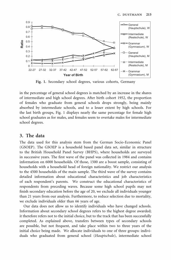
in the percentage of general school degrees is matched by an increase in the shares

of intermediate and high school degrees. After birth cohort 1952, the proportion

of females who graduate from general schools drops strongly, being mainly

absorbed by intermediate schools, and to a lesser extent by high schools. For

the last birth groups, Fig. 1 displays nearly the same percentage for female high

school graduates as for males, and females seem to overtake males for intermediate

school degrees.

3. The dataThe data used for this analysis stem from the German Socio-Economic Panel

(GSOEP). The GSOEP is a household based panel data set, similar in structure

to the British Household Panel Survey (BHPS), where households are surveyed

in successive years. The first wave of the panel was collected in 1984 and contains

information on 6000 households. Of those, 1500 are a boost sample, consisting of

households with a household head of foreign nationality. We restrict our analysis

to the 4500 households of the main sample. The third wave of the survey contains

detailed information about educational characteristics and job characteristics

of each respondent’s parents. We construct the educational characteristics of

respondents from preceding waves. Because some high school pupils may not

finish secondary education before the age of 20, we exclude all individuals younger

than 21 years from our analysis. Furthermore, to reduce selection due to mortality,

we exclude individuals older than 66 years of age.

Our data does not allow us to identify individuals who have changed schools.

Information about secondary school degrees refers to the highest degree awarded;

it therefore refers not to the initial choice, but to the track that has been successfully

completed. As explained above, transfers between types of secondary schools

are possible, but not frequent, and take place within two to three years of the

initial choice being made. We allocate individuals to one of three groups: indivi-

duals who graduated from general school (Hauptschule), intermediate school

c. dustmann 213

0

0.1

0.2

0.3

0.4

0.5

0.6

0.7

0.8

0.9

22-27 27-32 32-37 37-42 42-47 47-52 52-57 57-62 62-67

Year of Birth

Rat

ioGeneral(Hauptschule), W

Intermediate(Realschule), W

Grammar(Gymnasium), W

General(Hauptschule), M

Intermediate(Realschule), M

Grammar(Gymnasium), M

Fig. 1. Secondary school degrees, various cohorts, Germany

(Realschule), or high school (Gymnasium), respectively. Dropouts are allocated to

special schools, which we subsume under the category ‘general school’. Our final

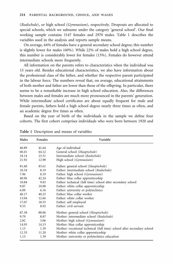
working sample contains 3147 females and 2970 males. Table 1 describes the

variables used in the analysis and reports sample means.

On average, 64% of females have a general secondary school degree; this number

is slightly lower for males (60%). While 22% of males hold a high school degree,

this number is considerably lower for females (13%). Females do however attend

intermediate schools more frequently.

All information on the parents refers to characteristics when the individual was

15 years old. Besides educational characteristics, we also have information about

the professional class of the father, and whether the respective parent participated

in the labour force. The numbers reveal that, on average, educational attainments

of both mother and father are lower than those of the offspring. In particular, there

seems to be a remarkable increase in high school education. Also, the differences

between males and females are much more pronounced in the parents’ generation.

While intermediate school certificates are about equally frequent for male and

female parents, fathers hold a high school degree nearly three times as often, and

an academic degree five times as often.

Based on the year of birth of the individuals in the sample we define four

cohorts. The first cohort comprises individuals who were born between 1920 and


Table 1 Description and means of variables

Males Females Variable

40.89 41.64 Age of individual60.41 64.12 General school (Hauptschule)18.14 23.31 Intermediate school (Realschule)21.92 12.98 High school (Gymnasium)

81.68 83.61 Father: general school (Hauptschule)10.34 8.19 Father: intermediate school (Realschule)7.96 8.19 Father: high school (Gymnasium)40.96 42.24 Father: blue collar apprenticeship10.84 9.83 Father: technical (full time) school after secondary school9.87 10.00 Father: white collar apprenticeship6.09 6.16 Father: university or polytechnics40.17 40.25 Father: blue collar worker13.04 12.66 Father: white collar worker17.07 18.53 Father: self employed9.53 8.92 Father: civil servant

87.38 88.06 Mother: general school (Hauptschule)9.79 8.87 Mother: intermediate school (Realschule)2.82 3.06 Mother: high school (Gymnasium)14.93 14.15 Mother: blue collar apprenticeship1.13 1.39 Mother: vocational technical (full time) school after secondary school12.35 11.20 Mother: white collar apprenticeship1.13 1.39 Mother: university or polytechnics education

1937. We chose this date because these individuals decided about secondary school

before or during the Second World War. Individuals in cohort 2 were born before

1946, and therefore entered secondary school during the first ten years after

World War Two. Individuals in cohort 3 were born before 1956, and individuals

in cohort 4 before 1966. Since our working sample is restricted to those individuals

who were at least 21 years of age in 1987, all individuals decided upon secondary

schools no later than 1975. Table 2 shows the cohort definition and the number of

cases in each cohort. The percentage of women in cohort one is slightly higher than

the percentage of men, which is a result of the Second World War as well as the

higher life expectancy of females.

4. Empirical analysisThe empirical analysis consists of five parts: first, we illustrate the transitions from

secondary school to post school education. Second, we analyse the association

between parents’ characteristics, and secondary school track of the individual.

Third, we illustrate changes over time, and point out differences between males

and females. Fourth, we investigate the association between educational achieve-

ments and wages. Fifth, we illustrate the impact of parental background on

the earnings of the individual via its influence on the secondary school track.

We estimate models where we allow parental characteristics to affect the child’s

wages by shifting probabilities of different secondary school tracks.

Our analysis does not attempt to answer questions like whether the higher

probability of high school attendance of children born to academic parents is

due to these children having higher learning abilities, or due to academically

educated parents tending to choose higher track secondary schools for the child.

To disentangle these effects creates serious identification problems, which we feel we

can not satisfactorily address with our data, due to lack of identifying information.

The coefficients we estimate are a combination of the two effects.

4.1 Secondary school choice and post school education

We argue above that the choice of the secondary school track is strongly associated

with later educational choices. In Tables 6 and 7 in the Appendix, we show cross

c. dustmann 215

Table 2 Definition of cohort dummies, number of cases

Males..............................

Females..............................

Variable Description Cases Mean Cases Mean

Cohort 1 Born between 1920 and 1936 886 25.30 886 28.34Cohort 2 Born between 1937 and 1946 750 25.81 732 23.76Cohort 3 Born between 1947 and 1956 624 21.48 690 22.40Cohort 4 Born between 1957 and 1966 796 27.40 785 25.48

tabulations for secondary school degrees and subsequent educational choices for

females and males, respectively. The numbers refer to the first three cohorts

only, since individuals in the fourth cohort may still be in education, predomi-

nantly at universities. The three panels distinguish between the three secondary

schools: general, intermediate, and high school. The variable ‘other’ summarises

individuals with post secondary education not included in any of the other

categories.

Table 3 displays Goodman–Kruskal correlation coefficients, which

summarise the cross tabulations. This coefficient is bounded between �1 and 1,

and can be interpreted as the difference in probability of like rather than

unlike responses for the two education measures when two individuals are

chosen at random. We have printed significant positive correlations in bold.

The numbers reflect the same pattern as the percentages in Tables 6 and 7 in

the Appendix.

The entries in the upper panel of Table 3 refer to males. They illustrate that

secondary school attendance for males is strongly associated with post-secondary

education. Having attended a secondary general school is strongly and significantly

correlated with subsequent blue-collar apprenticeship training. Intermediate school

graduates tend to obtain further education by attending technical schools, or join-

ing white collar apprenticeship schemes. Being a high school graduate is strongly

correlated with attending university. While the low occurrence of upward transi-

tions (from general school to university) is not so surprising, the numbers also

suggest that downward transitions are not frequent. The numbers in the last

block indicate that the association between high school degree, and a blue collar

apprenticeship is very low.

The numbers for females (lower panel) are similar. While males with general

secondary school degrees tend to enrol in blue-collar apprenticeships, and males

with intermediate school degrees in white collar apprenticeships or technical

schools, females from both intermediate and high schools tend to enrol in white

rather than blue collar apprenticeship schemes.

The numbers in Tables 6 and 7 in the Appendix show that the ratio of females

with a general school education and without further vocational training dropped

dramatically over cohorts. On the other side, the share of former general school

pupils in technical schools nearly doubles from cohort 1 to cohort 2. The fraction

of females and males with a general secondary school degree who decide to obtain

no further education drops systematically over cohorts.

The picture that emerges from these numbers is that for males there is a strong

association between general school degrees and blue-collar vocational training,

intermediate school degrees, and white-collar or vocational school training,

and high school and academic degrees. For females, both general and intermediate

school graduates tend to attend technical schools and white, rather than blue

collar apprenticeship schemes. These strong associations emphasise the importance

of secondary school choices for understanding subsequent choices within the

German educational system.


c. dustmann 217

Table

3C

orr

elat

ion

seco

nd

ary

sch

oo

l—p

ost

-sec

on

dar

yed

uca

tio

n

Secondary

Nofurther

education

.....

.....

.....

.....

.....

....

Bluecollar

apprenticeship

.....

.....

.....

.....

......

.....

..

Technical

school

.....

......

.....

.....

.....

..

Whitecollar

apprenticeship

.....

......

.....

.....

.....

.....

..

University

degree

.....

.....

.....

.....

.....

....

Other

.....

.....

.....

.....

......

...

education

Corr.

StdE.

Corr.

StdE.

Corr.

StdE.

Corr.

StdE.

Corr.

StdE.

Corr.

StdE.

Mal

esG

ener

al0.68

0.05

90.76

0.02

5�

0.30

0.05

2�

0.01

0.06

6�

0.97

0.00

7�

0.05

0.13

7In

term

edia

te�

0.68

0.09

2�

0.43

0.05

50.66

0.03

60.29

0.06

9�

0.42

0.08

60.

190.

154

Hig

hsc

ho

ol

�0.

690.

086

�0.

920.

020

�0.

480.

075

�0.

310.

089

0.98

0.00

3�

0.09

0.18

2

Fem

ales

Gen

eral

0.67

0.03

20.51

0.07

1�

0.10

0.04

8�

0.53

0.04

7�

0.99

0.00

7�

0.41

0.10

5In

term

edia

te�

0.59

0.04

3�

0.39

0.08

90.39

0.04

50.53

0.04

8�

0.43

0.11

90.

490.

098

Hig

hsc

ho

ol

�0.

800.

050

�0.

670.

124

�0.

680.

070

0.22

0.09

60.99

0.00

2�

0.05

0.23

5

Not

es:

Go

od

man

–K

rusk

alco

rrel

atio

nco

effi

cien

ts(s

tan

dar

der

rors

),co

mp

ute

das

�¼

ðP�

QÞ=ðP

þQÞ,

wh

ere

Pis

the

nu

mb

ero

fco

nco

rdan

t,an

dQ

the

nu

mb

ero

f

dis

cord

ant

pai

rso

fo

bse

rvat

ion

s.

4.2 Factors associated with secondary school choice

We now have a closer look at the association between parental characteristics, and

the children’s secondary school track. We model the allocation to secondary school

tracks as an ordered probit model, where we distinguish between the three cate-

gories of general, intermediate, and high school. We first estimate models for males

and females separately where we pool all cohorts. We allow for cohort effects in

a flexible way by introducing a polynomial of the year of birth of degree 4.8

Secondary school choice is explained by variables that reflect parents’ school and

post-school education, and variables about the father’s professional class.

To interpret the estimation results, we calculate the differential marginal effects

of explanatory variables on the probability that an individual attends high school or

intermediate school, as compared to general school.9 Table 4 presents the estimates

and standard errors. All effects are calculated for the average sample individual in

the respective subgroup.

There are several noteworthy results in Table 4. While for males, an intermediate

or high school degree held by the father increases the probability that the individual

attends high school by more than the probability that the individual attends inter-

mediate school (relative to general school), the opposite is the case for females.

This indicates that intermediate school attendance is considered to be a sufficient

education for female offsprings, while better educated fathers tend to send their

sons to a high school rather than an intermediate school. Interesting is also that

mother’s academic education is significantly associated with attending intermediate

or high school (relative to general school) for girls, but not for boys.

The variables that characterise the post school education of the father are all

significant and positive. Again, while any after school degree of the father increases

the probabilities of the son’s high school attendance more than the probability of

son’s intermediate school attendance, the opposite is the case for daughters. White

collar apprenticeship, or vocational after school education of the father affects

higher school track attendance of the individual more strongly than blue collar

after school education. As one should expect, the association between the child’s

higher secondary school track education and academic education of the father is

strong. The same patterns prevails for mother’s after school education.

All job characteristics of the father are strongly significant predictors for child’s

(relative) secondary school choice. Notice that coefficient estimates of father’s


..........................................................................................................................................................................8 The null hypothesis for equal parameters for both genders is rejected at the 5% level, using a likelihood-

ratio test. We therefore base our further analysis on gender specific estimations.9 These parameters are given by [2�(x0b)��(�� x0b)]b for intermediate vs general school, and by

[�(��x0 b)þ�(x0 b)]b for high school vs general school, where x is a vector of characteristics, b the

corresponding vector of parameter estimates, and � the density of the standard normal. The model is

normalised by setting its variance equal to one, so that � is the estimated threshold parameter. Standard

errors of these parameters can in principle be computed using the Delta method. Easier is computation

by simulation. We draw 500 observations of the estimated parameters b from their asymptotic normal

distribution, and compute the standard errors of the predicted differential marginal probabilities.

c. dustmann 219

Table

4M

argi

nal

dif

fere

nti

alef

fect

so

fp

aren

ts’

char

acte

rist

ics

Males

.....

.....

......

.....

.....

.....

.....

......

.....

.....

.....

.....

......

.....

.....

.....

.....

......

.Fem

ales

.....

.....

.....

.....

......

.....

.....

.....

.....

......

.....

.....

.....

.....

......

.....

.....

.....

..

Interm

ediate

vs.general

.....

.....

......

.....

.....

.....

.....

....

Highschool

vs.general

....

......

.....

.....

.....

.....

......

....

Interm

ediate

vs.general

.....

.....

.....

.....

......

.....

.....

....

Highschool

vs.general

.....

......

.....

.....

.....

.....

.....

....

Variable

Coeff.

StdE.

Coeff.

StdE.

Coeff.

StdE.

Coeff.

StdE.

Fat

her

hig

hsc

ho

ol

0.27

50.

072

0.34

30.

090

0.35

90.

074

0.29

70.

061

Fat

her

inte

rmed

sch

oo

l0.

286

0.04

50.

357

0.05

50.

273

0.05

40.

226

0.04

4M

oth

erh

igh

sch

oo

l0.

360

0.10

60.

450

0.13

30.

282

0.11

50.

234

0.09

5M

oth

erin

term

edsc

ho

ol

0.26

00.

053

0.32

50.

068

0.20

40.

058

0.16

90.

048

Fat

her

acad

emic

ed0.

546

0.08

40.

682

0.10

40.

471

0.08

60.

390

0.07

1F

ath

erb

lue

col.

app

r.0.

175

0.03

80.

219

0.04

70.

147

0.04

20.

121

0.03

4F

ath

erw

hit

eco

l.ap

pr.

0.30

20.

056

0.37

70.

069

0.34

20.

060

0.28

30.

049

Fat

her

tech

nic

alsc

h.

0.22

90.

055

0.28

60.

068

0.30

80.

062

0.25

40.

051

Mo

ther

acad

emic

ed0.

041

0.13

10.

051

0.16

40.

376

0.13

90.

311

0.11

4M

oth

erb

lue

col.

app

r.0.

072

0.03

80.

090

0.04

70.

022

0.04

30.

018

0.03

6M

oth

erw

hit

eco

l.ap

pr.

0.12

00.

039

0.15

00.

048

0.19

80.

045

0.16

40.

037

Mo

ther

tech

nic

alsc

h.

�0.

002

0.11

3�

0.00

30.

141

0.20

70.

123

0.17

10.

102

Fat

her

wh

ite

coll

arjo

b0.

198

0.04

50.

247

0.05

60.

309

0.05

00.

255

0.04

1F

ath

erse

lfem

plo

yed

0.18

20.

039

0.22

70.

049

0.25

90.

041

0.21

40.

033

Fat

her

civi

lse

rvan

t0.

301

0.05

40.

375

0.06

70.

322

0.06

00.

266

0.05

0Y

ear

bo

rn/1

0�

2.76

92.

107

�3.

456

2.62

5�

4.65

22.

235

�3.

849

1.84

0Y

ear

bo

rn2/1

0310

.191

7.82

212

.719

9.74

719

.861

8.49

016

.431

6.99

1Y

ear

bo

rn3/1

05�

15.0

1512

.453

�18

.743

15.5

20�

33.5

8713

.794

�27

.787

11.3

55Y

ear

bo

rn4/1

077.

739

7.19

49.

662

8.96

719

.957

8.11

316

.510

6.67

8

Not

es:

Ord

ered

pro

bit

mo

del

s.M

argi

nal

dif

fere

nti

alef

fect

san

dth

eir

stan

dar

der

rors

are

rep

ort

ed.

professional characteristics are conditional on father’s educational achievement.

Accordingly, the working environment and the associated social relations and

peer group of the father seem to play an important role for the secondary school

education of the child.

These estimates suggest that the association between parental educational

attainment and profession and the secondary track education the child follows is

substantial. The estimates show some interesting differences between males and

females: characteristics of parents which are strongly associated with a high school

education for males, are strongly associated with intermediate school education

for females. This is in line with the relative overall tendency of females to enrol in

intermediate schools, as depicted in Fig. 1.

4.3 Changes in secondary school education

We now illustrate changes in the probabilities of track choice over time. We

simulate school track attendance probabilities for parents with different educa-

tional background, and different professional class, based on the estimates in the

previous section. We allow for changes in educational choices of individuals of the

same parental background, according to the cohort individuals are born into,

which is captured by a cohort polynomial.10

We choose two parental background scenarios: A typical working class family,

and a family with academic background. We define parental working class back-

ground as a father with general secondary school education, blue collar apprentice-

ship and a blue collar job, and a mother with general secondary school education.

We define an academic background as a father who has a high school degree, an

academic degree, and a white collar job, and a mother who has a high school degree

and an academic education.

Probabilities for individuals who come from a family with typical working class

background are displayed in Fig. 2, and for individuals from an academic back-

ground in Fig. 3. The figures illustrate the evolution of probabilities of general,

intermediate and high school attendance according to birth year, for birth cohorts

between 1921 and 1966. Solid lines represent males, and dashed lines represent

females. The lines for the various school types carry different symbols, which are

explained in the figures.

The figures show the dramatic differences in probabilities of high school

attendance for individuals with different parental background. While the probabil-

ity of high school attendance is always below 20% for a male working class indi-

vidual, it is always above 70% for an individual with academic family background.

For individuals with working class background, a decline in the share of general

school education is visible, accompanied by an increase in intermediate and high

schools. This is more pronounced for females than for males. For individuals with

academic background, the probability of attending high school is about 60% for


..........................................................................................................................................................................10 For both males and females, the polynomial terms are jointly significant at the 1% level.

c. dustmann 221

Fig. 2. School attendance probabilities, working class parents

Fig. 3. School attendance probabilities, academic parents

females, and 80% for males, for the cohort born in 1921. For males, this probability

is relatively stable over time, with only a slight increase in the second half of the

last century. For females, there is a strong increase, and probabilities equalise with

those for males for the 1960s cohorts. On the other hand, the probability of general

school education is never higher than 10%, and it approaches zero for both genders

in the last cohort.

The figures suggest low educational mobility, with a tendency towards limited

convergence of school allocations across family backgrounds over time.

Furthermore, they illustrate an overall shift towards better education for females,

and a closing gap between males and females during the second half of the last

century.

4.4 Educational achievements and wages

In the last section, we have illustrated that parental background is strongly related

to educational achievements of the child. In this section, we investigate how educa-

tional achievements are associated with wages. In the next section, we analyse how

parental background affects wages, via its association with educational attainments.

We de-trend wages first by making use of administrative longitudinal data for

Germany (see Bender et al., 1996, for details on this data). We construct a sample

of young workers, whose first spell in the labour market we observe for the years

1984–1990 (see Dustmann and Meghir, 2004, for details on this data). Variation in

entry wages of these workers are due to variation in educational background and

entry year only, since their labour market experience is equal to zero. We use the

estimated time effects from wage regressions of this sample of entrants to de-trend

wages for the first seven years of the panel (between 1984 and 1990). We then

estimate wage regressions, conditioning on educational achievements, an age

polynomial, and cohort dummies, which are defined according to the classification

in Table 1. The panel information allows us to identify both cohort- and age effects.

The wage equations we estimate are given by

ln wgit ¼ �

g0 þ �

g1ischi þ �

g2gschi þ �

g3cohi þ PiðageÞ�g þ TR0

i�g þ uit ð1Þ

where ln w is the log of (de-trended) wages, isch and gsch are dummy variables for

intermediate and high school attendance, coh are cohort dummies, TR is a vector of

further educational achievements, and P(age) is a polynomial in age of degree 3.

The indices i, t, g stand for individuals, time, and gender. We define the coefficients

to be such that Eðuit j isch; gsch; coh; PðageÞ;TRÞ ¼ 0.

In columns 1 and 3 of Table 5, we display estimates where we condition on

secondary school education, as well as after-secondary school attainments. Omitted

category is individuals with a general school degree, and no further training.

According to these estimates, an intermediate school degree is associated with an

increase in log wages of 0.15 and 0.24 for males and females, respectively. A high

school degree is associated with an increase in log wages by about 0.26 (males) and

0.32 (females).


Blue collar and white collar apprenticeships, as well as vocational school atten-

dance lead to further increases in the expected wage, with white collar apprentice-

ships having the largest coefficients for both genders. University education adds

substantially to after-secondary school wages for both genders.

The cohort dummies are significant for males, indicating that (compared to the

first cohort) wages in cohorts 2 and 3 are slightly higher. Wages in cohort 4 are

lower again, which may be due to the fact that many university graduates in this

cohort have not entered the labour market yet. For females, cohort effects are

mostly insignificant.

In columns 2 and 4, we present results where we regress on secondary

school degrees only. The coefficients can be interpreted as the association between

the respective secondary school degree and wages for an individual with

expected further educational achievements, conditional on having achieved a

particular secondary school degree. General school attainment (and expected

further training achievements associated with general school attainment) is the

reference group.

As expected, coefficients for the two school categories increase, and are slightly

larger for females. Compared to a male individual with general schooling (and the

associated average further training), a high school graduate (with average weighted

further educational achievements) earns about 54% (calculated as (e0.433�1))

higher wages. In the next section, we take this specification as a starting point.

We investigate how parental characteristics, via their impact on secondary school

attainments, affect wages of individuals.

c. dustmann 223

Table 5 Wage regressions

Males.........................................................

Females.........................................................

1..........................

2..........................

3..........................

4..........................

Variable Coeff. StdE. Coeff. StdE. Coeff. StdE. Coeff. StdE.

Constant 1.611 0.155 1.246 0.160 2.196 0.239 1.324 0.246Intermediate school 0.148 0.007 0.196 0.006 0.236 0.010 0.289 0.010High school 0.257 0.010 0.433 0.006 0.317 0.016 0.546 0.012Blue collarapprenticeship

0.105 0.008 – – 0.026 0.015 – –

White collarapprenticeship

0.180 0.010 – – 0.165 0.010 – –

Vocational training 0.142 0.009 – – 0.159 0.013 – –University education 0.378 0.013 – – 0.499 0.021 – –age/10 0.493 0.133 0.857 0.137 �0.182 0.207 0.574 0.213age2/103

�0.606 0.353 �1.470 0.364 1.158 0.561 �0.661 0.579age3/105 0.140 0.295 0.795 0.304 �1.391 0.477 �0.023 0.494cohort 2 0.054 0.015 0.054 0.015 �0.065 0.026 �0.073 0.027cohort 3 0.070 0.024 0.063 0.024 �0.019 0.040 �0.035 0.041cohort 4 0.036 0.029 0.015 0.030 0.007 0.048 �0.012 0.050N. Obs. 12598 12598 7738 7738

4.5 Wages and parental background

We have illustrated in Section 4.3 that there is some convergence in educational

track choice over cohorts between individuals with different parental background.

We now simulate how this translates into log wages, via its effect on the secondary

school choice of the individual. We predict log wages, conditional on parental

background only. This corresponds to expected wages, conditional on a set of

parental background information PB

Eðln w jPBÞ ¼ e��0 þe��1 Eðisch j PBÞ þe��2Eðgsch j PBÞ

¼ e��0 þe��1Probðisch j PBÞ þe��2Probðgsch j PBÞ

Based on this specification, we predict log wages for individuals in 1987 with the

same parental background, but born in different years. We eliminate the direct

time and cohort effects on wages by conditioning on cohort dummies, and by

de-trending wages first, as explained above. Age in 1987 influences wages in our

simulations in two ways: First, by positioning individuals on their life cycle log

wage-age profile. The wage-age profile is assumed to be the same for individuals

with different educational background. Second, by the cohort effect on educational

attainments. Individuals with the same parental background may achieve different

secondary school attainments, according to their cohort, as we have illustrated

in Section 4.3. This second effect affects individuals with different parental

background differently, and it may thus lead to convergence or divergence of

profiles.

We consider again an individual from a working class background, and an

individual from an academic background, where we use the same definitions as

in the previous section.

We obtain the probabilities Prob(isch j PB) and Prob(gsch j PB) from our ordered

probit model. In Figs 4 and 5, we plot the predicted wage profiles for males and

females, respectively. In Table 8 in the Appendix, we report the wage differences

(according to parental background) for the various age groups, and the t-ratios of

the differences between wages at different ages for individuals from academic and

working class background.11

Wage differentials for individuals with different parental background are size-

able. For males who are 26 years old in 1987, the log wage differential between

an individual born into an academic family and an individual born into a working

class family is about 0.3, translating into a 35% differential. For females, the

differential is larger at 46%.


..........................................................................................................................................................................11 To compute the standard errors, we take account of the fact that the parameters in the wage equation,

as well as the parameters in the ordered probit model (used to form the predictions of secondary school

attendance) are random variables. Computation of the standard errors is based on simulations.

c. dustmann 225

Fig. 4. Wage profiles, males

Fig. 5. Wage profiles, females

The figures indicate only a slight convergence in wage profiles of individuals

in younger cohorts, relative to older cohorts, due to convergence in educational

achievements of individuals with different parental background. On average, male

individuals from a working class background and born in 1961 obtain wages which

are about 35% lower than those of individuals from an academic background; this

difference increases by only 2.3% for individuals born in 1932. The increase is due

to the larger relative disadvantage in acquiring higher track education for indivi-

duals from working class background who were born in 1932, compared to those

born in 1961. Thus, the slight convergence we observe in terms of secondary

track education between individuals of different background translates in a small

convergence in wages.

Again, notice that our analysis does not identify causal effects. There are many

reasons why later earnings capacity may be linked to parental background. Parental

background may be correlated with individuals’ unobserved ability in the

educational outcome equation. It may also be correlated with unobservables in

the wage equation, either via ability, or via network effects or personal contacts.

Our estimates refer to the composite of all these effects.

5. Conclusion and discussionIn this paper, we argue that an important factor for explaining intergenerational

mobility of income status and education is the influence parents may have on early

school track decisions of the child. This, in turn, is related to institutional features

of the education system, in particular the age at which the secondary school track

choice has to be taken. In Germany, primary, secondary, and post-school education

is state provided, tuition-free, and there are no large differences in quality across

schools of a given track. Despite that, we document a substantial immobility

of educational achievement across generations. We also find that differences in

parental background translate, via their association with secondary track school

choice, into sizeable wage differences.

One reason for this may be the relatively young age at which the secondary

track decision has to be taken, giving a high weight to parental preferences. This

particular feature of the German education system has been mostly overlooked,

with researchers focussing on post secondary education, and first transitions into

the labour market.

A key question has not been addressed so far. In the absence of tuition fees for

secondary schools (at least for recent cohorts), and no selective entry tests, why do

not all parents send their children to upper track schools? And if there is differential

allocation, why should it be related to educational background of the parent? There

are various possible explanations. Although it is the parent who ultimately decides

about the child’s secondary track, there are, as we point out above, recommenda-

tions by the primary school teacher. Parents with weaker educational background

may be less confident, and consider these recommendations as more binding


than parents with higher educational background. Furthermore, at so low an age

children may not yet have fully revealed their academic potential. Better educated

parents may be in a stronger position to extract information about this potential,

and decide for higher track schools despite a negative recommendation of

the teacher. Also, better educated parents may feel that they have more resources

(both financially and in terms of academic advice) to support their child at a

higher track secondary school than parents with poorer educational background.

Peer pressure may be another explanation for education-dependent parental

decisions.

Finally, professional traditions may play an important role. These traditions

are strongly developed in Germany, in particular in the craft sector. Parents’ own

education and professional class may shape their taste and perception of what is

an appropriate educational and professional career for the child. Even in the

absence of financial constraints, working class parents may consider a lower track

education and an early labour market entry the best option for their child.

In addition, knowledge transmission may contribute to occupational persistence

across generations, in particular in the craft sector. Lentz and Laband (1989)

and Laband and Lentz (1992) among others provide evidence for occupational

inheritance.

We have not tested these explanations—this is left for future research. We believe

however that the way parents take part in educational choices of their children

is crucial for our understanding of intergenerational mobility. In this paper we

emphasise the age of secondary track choice as a possible key factor, and provide

evidence of strong intergenerational immobility of educational achievements in

a country where this decision is taken very early on.

Acknowledgements

I am grateful to Wendy Carlin, John Micklewright, and two anonymous referees for usefulcomments on earlier versions of this paper.

References

Bender, S., Hilzendegen, J., Rohwer, G., and Rudolph, H. (1996). ‘Die IAB Beshaeftigungs-stichprobe 1975–1990’, Beitraege zur Arbeitsmarkt- und Berufsforschung, BeitrAB 197,Nurnberg.

Ben-Porath, Y. (1967). ‘The production of human capital and the life cycle of earnings’,Journal of Political Economy, 75, 352–65.

Buechel, F., Frick, J.R., Krause, P., and Wagner, G. (2000). ‘The impact of povertyon childrens’ school attendance—evidence from West Germany’, mimeo, Department ofEconomics, University of Berlin.

Bjoerklund, A. and Jaenti, M. (1997). ‘Intergenerational mobility in Sweden compared withthe United States’, American Economic Review, 87, 1021–8.

Buechtemann, C.F., Schupp, J., and Soloff, D. (1993). ‘Roads to work: school-to-worktransition patterns in Germany and the United States’, Industrial Relations Journal, 24,97–111.

c. dustmann 227

Caterall, J. (1998). ‘Risk and Resilience in student transitions to high school’, AmericanJournal of Education, 106, 302–33.

Couch, K.A. (1994). ‘High school vocational education, apprenticeship, and earnings: acomparison of Germany and the United States’, Vierteljahreshefte zur Wirtschaftsforschung,Heft 1, 10–18.

Dearden, L., Machin, S., and Reed, H. (1997). ‘Intergenerational mobility in Britain’,The Economic Journal, 107, 47–64.

Dustmann, C. and Meghir, C. (2004). ‘Wages, experience, and seniority’, Review of EconomicStudies, forthcoming.

Ermisch, J. and Francesconi, M. (2001). ‘Family matters: impacts of family background oneducational attainments’, Economica, 68, 137–56.

Feinstein, L. and Symons, J. (1999). ‘Attainment in secondary school’, Oxford EconomicPapers, 51, 300–21.

Galton, M., Gray, J., and Rudduck, J. (1999). ‘The impact of school transitions andtransfers on pupil progress and attainment’, Department for Education and Employment,1–37.

Jenkins, S. (1987). ‘Snapshots versus movies: ‘‘lifecycle biases’’ and the estimation ofintergenerational earnings inheritance’, European Economic Review, 31, 1149–58.

Jenkins, S. and Schlueter, C. (2002). ‘The effect of family income during childhood onlater-life attainment: evidence from Germany’, Discussion Paper No. 604, IZA, Berlin.

Laband, D.N. and Lentz, B.F. (1992). ‘Self-recruitment in the legal profession’, Journalof Labor Economics, 10, 182–201.

Lentz, B.F. and Laband, D.N. (1989). ‘Why do so many children of doctors become doctors’,Journal of Human Resources, 24, 392–413.

Merz, M. and Schimmelpfennig, A. (1999). ‘Career choices of German high schoolgraduates: evidence from the German socio-economic panel’, Working Paper No. 99/11,European University Institute, Florence.

OECD (2000). Knowledge and Skills for Life—First Results from Pisa 2000, available online atwww.pisa.oecd.org/Docs/Download/PISAExeSummary.pdf

Pischke, J.S. (1999). ‘Does shorter schooling hurt student performance and earnings?Evidence from the German short school years’, mimeo, MIT, Cambridge, MA.

Riphahn, R. (1999). ‘Residential location and youth unemployment: the economicgeography of school-to-work- transitions’, mimeo, Department of Economics, Universityof Munich.

Ryan, P. (2000). ‘The institutional requirements of apprenticeship: evidence from smallerEU countries’, International Journal of Training and Development, 4(1), 42–65.

Ryan, P. (2001). ‘The school-to-work transition: a cross-national perspective’, Journal ofEconomic Literature, 39, 34–92.

Sanderson, M. (1994). Missing Stratum: Technical School Education in England 1900–1990s,Continuum International Publishing Group, London.

Shavit, Y. and Mueller, W. (1998). ‘The institutional embededness of the stratificationprocess: a comparative study of qualifications and occupations in thirteen countries’,in Y. Shavit and W. Mueller (eds), From School to Work: A Comparative Study ofEducational Qualifications and Occupational Destinations, ch. 1, Clarendon Press, Oxford.


Statistisches Bundesamt (1994). Statistisches Jahrbuch fur die Bundesrepublik Deutschland,Wiesbaden.

Steedman, H. (1993). ‘The economics of youth training in Germany’, Economic Journal, 103,1279–91.

Solon, G. (1992). ‘Intergenerational income mobility in the United States’, AmericanEconomic Review, 82, 393–408.

Solon, G. (1999). ‘Intergenerational mobility in the labour market’, in O. Ashenfelterand D. Card (eds), Handbook of Labor Economics, Vol. 3A, North Holland, Amsterdam.

Soskice, D. (1994). ‘The German training system: reconciling markets and institutions’,in L. Lynch (ed.), International Comparisons of Private Sector Training, NBER conferencevolume, University of Chicago Press, Chicago, IL.

Wiegand, J. (1999). ‘Four essays on applied welfare measurement and income distributiondynamics in Germany 1985–1995’, PhD-Thesis, University College London.

Winkelmann, R. (1996a). ‘Training, earnings and mobility in Germany’, Konjunkturpolitik,42, 275–98.

Winkelmann, R. (1996b). ‘Employment prospects and skill acquisition ofapprenticeship trained workers in Germany’, Industrial and Labor Relations Review,49(4), 658–72.

Zimmerman, D. (1992). ‘Regression towards mediocrity in economic stature’, AmericanEconomic Review, 82, 409–29.

Appendix

c. dustmann 229

Table 6 Transitions secondary–after secondary education, males

Secondaryeducation

Cohort No after-sec.education

Bluecollar

Vocationalschool

Whitecollar University Other No. Obs.

General Cohort 1 18.04 53.92 12.94 11.37 1.18 2.55 510secondary Cohort 2 14.79 53.45 13.21 14.40 0.99 3.16 507school Cohort 3 10.92 53.50 18.21 15.13 0.28 1.96 357

All 14.99 53.64 14.41 13.46 0.87 2.62 1374

Intermediate Cohort 1 5.45 17.27 43.64 20.00 7.27 6.36 110secondary Cohort 2 1.75 27.19 43.86 14.91 8.77 3.51 114school Cohort 3 0.81 23.39 41.13 25.81 7.26 1.61 124

All 2.59 22.70 42.82 20.40 7.76 3.74 348

High Cohort 1 0.00 4.35 15.65 9.57 66.96 3.48 115school Cohort 2 0.78 3.10 3.10 9.30 80.62 3.10 129

Cohort 3 6.29 2.80 6.29 6.29 77.62 0.70 143All 2.58 3.36 8.01 8.27 75.45 2.33 387

Note: The column entries refer to percentages of respective after-secondary school education for the

different secondary attainments. We distinguish between no further education, blue collar apprentice-

ship, vocational school, white collar apprenticeship, and university. For each cohort the numbers in a

row add up to 100.


Table 8 Wage differentials high/low educational background

Males.......................................

Females.......................................

Age �lnw t-ratio �lnw t-ratio

26 0.297 17.63 0.379 13.8027 0.299 19.32 0.385 15.2028 0.301 21.19 0.390 16.7529 0.302 23.27 0.395 18.4930 0.305 25.60 0.400 20.4331 0.307 28.17 0.405 22.5932 0.309 30.91 0.409 24.9233 0.311 33.58 0.412 27.2434 0.313 35.77 0.414 29.2135 0.314 36.93 0.416 30.3036 0.316 36.61 0.418 30.1137 0.317 34.86 0.418 28.6038 0.318 32.15 0.418 26.2539 0.319 29.10 0.418 23.5840 0.319 26.11 0.418 21.0241 0.320 23.42 0.417 18.7342 0.320 21.08 0.416 16.7643 0.320 19.08 0.415 15.1044 0.320 17.40 0.414 13.7245 0.320 15.97 0.414 12.5646 0.320 14.77 0.413 11.5847 0.320 13.75 0.413 10.7648 0.320 12.88 0.412 10.0649 0.320 12.14 0.412 9.46550 0.320 11.50 0.412 8.94651 0.320 10.95 0.412 8.49052 0.320 10.48 0.412 8.08453 0.320 10.06 0.412 7.71554 0.320 9.699 0.413 7.37255 0.320 9.369 0.413 7.046

Table 7 Transitions secondary–after secondary education, females

Secondaryeducation Cohort

No after-sec.education

Bluecollar

Vocationalschool

Whitecollar University Other No. Obs.

General Cohort 1 62.43 11.09 17.60 6.95 0.00 1.92 676secondary Cohort 2 44.22 15.11 29.10 8.96 0.19 2.43 536school Cohort 3 29.76 15.95 45.48 6.90 0.24 1.67 420

All 48.04 13.66 28.55 7.60 0.12 2.02 1632

Intermediate Cohort 1 28.37 9.22 36.17 17.73 3.55 4.96 141secondary Cohort 2 10.14 2.03 54.73 24.32 2.70 6.08 148school Cohort 3 11.93 6.25 44.32 28.98 2.27 6.25 176

All 16.34 5.81 45.16 24.09 2.80 5.81 465

High Cohort 1 7.14 5.36 10.71 19.64 51.79 5.36 56school Cohort 2 6.25 2.08 6.25 18.75 64.58 2.08 48

Cohort 3 7.45 1.06 7.45 13.83 69.15 1.06 94All 7.07 2.53 8.08 16.67 63.13 2.53 198

Note: The column entries refer to percentages of respective after-secondary school education for the

different secondary attainments. We distinguish between no further education, blue collar apprentice-

ship, vocational school, white collar apprenticeship, and university. For each cohort the numbers in a

row add up to 100.

parental background, secondary school track choice, and - ucl

Documents