parametric study of two-phase flow by integral analysis

Journal of Mechanical Science and Technology 24 (7) (2010) 1379~1387

www.springerlink.com/content/1738-494x DOI 10.1007/s12206-010-0419-z

Parametric study of two-phase flow by integral analysis

based on power law distribution† Woo Gun Sim1,*, N. W. Mureithi2 and M. J. Pettigrew2

1Department of Mechanical Engineering, Hannam University, Taejeon 306-791, Korea 2Department of Mechanical Engineering, École Polytechnique, Montreal H3T 1J4, Canada

(Manuscript Received April 28, 2009; Revised March 11, 2010; Accepted March 22, 2010)

----------------------------------------------------------------------------------------------------------------------------------------------------------------------------------------------------------------------------------------------------------------------------------------------

Abstract To understand the fluid dynamic forces acting on a structure subjected to two-phase flow, it is essential to obtain detail information on

the characteristics of that flow. The distributions of flow parameters across a pipe, such as gas velocity, liquid velocity and void fraction, may be assumed to follow a power law (Cheng 1998; Serizawa et al. 1975). The void fraction profile is, for example, uniform for bubbly flow, whereas for slug flow it is more or less parabolic. In the present work, the average values of momentum flux, slip ratio and other parameters were derived by integral analysis, based on approximate power law distributions. A parametric study with various distribu-tions was performed. The existing empirical formulations for average void fraction, proposed by Wallis (1969), Zuber et al. (1967) and Ishii (1976), were considered in the derivation of the present results. Notably, the unsteady momentum flux for slug flow was approxi-mated.

Keywords: Annular flow; Bubbly flow; Drift flux model; Homogeneous model; Momentum flux of two-phase flow; Momentum multiplier; Slug flow;

Void fraction ---------------------------------------------------------------------------------------------------------------------------------------------------------------------------------------------------------------------------------------------------------------------------------------------- 1. Introduction

Two-phase vapour-liquid flow exists in many shell and tube heat exchangers such as steam generators in Nuclear Steam Supply Systems. Two-phase hydrodynamic forces have been studied by Carlucci [1], Carlucci and Brown [2] and Pettigrew et al. [3-5], and single-phase flow has been examined by Fritz [6] and Price [7]. However, more information on the physical behaviour of two-phase flow, especially with respect to flow-induced vibration, is required. Depending on the flow regime, one might find gas bubbles, liquid drops, slugs, or waves in two-phase flow (Jones & Zuber [8]; Legius et al. [9]; Sim[10]). These are all accompanied by severe fluctuations in pressure, void fraction and momentum flux. Knowledge of these fluc-tuations is pertinent to the development of two-phase flow technology and its application to engineering problems related to flow-induced vibration. In order to investigate flow-induced vibration, it is essential to understand flow regime. Flow-regime conditions usually are represented in terms of dimen-sionless parameters in the form of a flow regime map.

One of the earliest and most reliable correlations for pres-

sure drop arising from the flow of gas-liquid mixtures in a pipe was derived by Lockhard & Martinelli [11]. This empiri-cal method was assumed to be valid over all flow regimes. To predict void fraction in co-current gas-liquid flows, several models have been proposed (Baroczy [12], Turner & Wallis [13]). The similarity between the models was shown, and a new empirical formulation for void fraction correlation was proposed, by considering the existing test results (Butterworth [14]). The most relevant and useful of these methods are those which attempt to model the particular hydrodynamic features of the flow; accordingly, the treatments are loosely grouped under the various flow patterns: bubbly flow, bubbly-slug flow, slug flow and annular flow. In bubbly and slug flow, the gas velocity is affected by the tendency of the bubbles to rise through the center of the pipe, where the local mixture veloc-ity is higher than the average velocity. The drift flux model, starting from an analytical approach, was developed by Zuber and Findlay [15]. The model was later extended for the vari-ous flow patterns (Ishii et al. [16]; Zuber et al. [17]; Wallis [18]).

To provide sufficient information on two-phase flow in a pipe, the void fraction and gas and liquid velocity profiles were measured by a cross-correlation technique by Cheng et al. [19] and Serizawa et al. [20]. The results show that the distribution of void fraction is a strong function of flow pat-

† This paper was recommended for publication in revised form by Associate EditorGihun Son

*Corresponding author. Tel.: +82 42 629 8089, Fax: 82 42 629 8293 E-mail address: [email protected]

© KSME & Springer 2010

1380 W. G. Sim et al. / Journal of Mechanical Science and Technology 24 (7) (2010) 1379~1387

tern and that it changes from a saddle-shaped to a parabolic-shaped distribution as the gas velocity or the flow quality in-creases; an exception to this is the region near the wall. In air-water flow, a saddle-shaped distribution corresponds to bub-bly flow, whereas a parabolic-shaped one correlates to slug flow. In general, the distributions for homogeneous flow are assumed to be uniform across the pipe.

To understand the dynamic characteristics of two-phase flow, parameter spectra have been measured by multi-channel techniques. It was demonstrated that the probability density function of the void fraction fluctuations could be used as an objective and quantitative flow pattern discriminator for the three dominant patterns of bubbly, slug and annular flow [8]. A correlation for the dominant frequency in slug flow was formulated by Heywood & Richardson [21]. The frequency was determined from a probability density function of instan-taneously measured liquid holdup. γ -ray absorption was used to measure the liquid holdup in a pipe of circular cross-section. It was found that the dominant frequency depends linearly on the superficial water flow velocity only, independ-ent of gas velocity for superficial velocities below 10 m/s (Leguis et al. [9]; Azzopardi & Baker [22]).

To understand the nature of the fluid dynamic forces acting on a structure subjected to two-phase flow, it is essential to obtain detailed information on the characteristics of that flow. Interest in momentum flux has arisen primarily from applica-tions in which this term is large. Measurement of momentum flux through a section of pipe with steam-water and air-water flows was reported by Andeen & Griffith [23], who used the results to evaluate the usefulness of various two-phase flow models. To provide basic information related to flow-induced vibration, an effort was made to explore the effects of geome-try, pressure, and flow rate on the momentum flux. In the pre-sent study, the distributions of flow parameters such as gas velocity, liquid velocity and void fraction[19, 20] across a pipe were assumed to follow a power law. The objective of this study was to determine the two-phase flow parameters and to compare the values with the predictions of various existing models. For this purpose, the momentum flux and the average quantities of two-phase flow were derived by integral analysis based on the power law. A parametric study with various dis-tributions was performed for the given average void fraction. To obtain the average void fraction, the existing empirical formulations proposed by Ishii [16], Zuber et al. [17] and Wal-lis [18], are used. Notably, a new model for the unsteady mo-mentum flux of slug flow was developed. This model employs the results of the present integral analysis and the frequency correlation suggested by Heywood & Richardson [21].

2. Drift flux model for two-phase flow in pipe

2.1 Initiation of present model

The homogeneous and separated flow models are the two most widely tested approaches to modeling two-phase flow

available at present. Schrage et al. [24] made void fraction measurements in an in-line bundle with air-water cross-flow using quick-closing plate valves. They found that the void fraction varies with mass flux and is greatly over-predicted by the homogeneous equilibrium model (HEM). This model ne-glects the effect of the velocity ratio between the phases. In vertical upward bubble and slug flow, the gas velocity is af-fected by the tendency of the bubbles to rise through the cen-ter of the pipe, where the local mixture velocity is higher than the average velocity. In low-velocity bubbly flow in large vertical pipes, the relative motion between the bubbles and the liquid is governed by a balance between buoyancy and drag forces; that is, the relative motion is a function of void fraction but not of flow rate. The drift-flux model U(UZuber & Findlay [15]) UiUs essentially a separated-flow model where attention is focused on the relative motion between phases rather than on the motion of the individual phases. The drift-flux theory has widespread applications to bubbly, slug, and droplet flow regimes of gas-liquid flow as well as to fluid-particle systems such as fluidized beds.

It is difficult to determine the average density, void fraction and effective flow velocity accurately, because these depend on the velocity ratio, S, which is defined as the ratio of gas to liquid-phase velocity. These parameters are needed, for in-stance, to understand flow-induced vibration and predict fluid forces in pipes subjected to two-phase flow. In the present study, the average values of the parameters were calculated by integral analysis based on the proposed power law distribu-tions for flow parameters across the pipe. It is known, for in-stance, that the void fraction profile is uniform for bubbly flow whereas it is more or less parabolic for slug flow. Exploiting these power law profiles, the Reynolds transport theorem was used to formulate the momentum flux acting on the pipe. To formulate the unsteady momentum of slug flow, the results of the present integral analysis and the frequency correlation suggested by Heywood and Richardson [21] were utilized.

2.2 Power laws for flow parameter distributions

As mentioned above, the distribution of the void fraction is a strong function of the flow pattern. Outside of the wall re-gion, the distribution changes from a saddle-shaped profile to a parabolic-shaped one as the gas velocity or quality in-creases (Cheng et al. [19]; Serizawa et al. [20]). As already mentioned, in air-water flow, a saddle-shaped distribution corresponds to bubbly flow, and a parabolic shape to slug flow. Similar distributions for bubble velocity are obtained. In gen-eral, the distributions for homogeneous flow are assumed to be uniform across the pipe. An example given by Cheng et al. is shown in Fig. 1.

In the present study, the distributions of flow parameters across a pipe, including gas velocity, gLu , liquid velocity,

fLu , and void fraction, Lα , were assumed to follow a power law. The subscripts g, f and L stand for gas, liquid and local, respectively. This approximation is valid if adherence or re-

W. G. Sim et al. / Journal of Mechanical Science and Technology 24 (7) (2010) 1379~1387 1381

bounding of bubbles at the surface of the wall is neglected. The power law distributions take the form

1

max

1n

fL

f o

u ru r

⎛ ⎞⎟⎜ ⎟= −⎜ ⎟⎜ ⎟⎜⎝ ⎠,

1

max

1m

gL

g o

u ru r

⎛ ⎞⎟⎜ ⎟= −⎜ ⎟⎜ ⎟⎜⎝ ⎠,

1

max

1p

L

o

rr

αα

⎛ ⎞⎟⎜ ⎟= −⎜ ⎟⎜ ⎟⎜⎝ ⎠ (1)

1Bwhere the subscript “max” denotes the maximum values at the center of the pipe, r=0. The integers (m, n and p ) are a priori unknown. Their values can, however, be estimated from ex-perimental data such as those shown in Fig. 1. In the present work, a parametric study was performed. Hence, m, n & p varied over a certain range and the resulting flow properties studied.

2.3 Average values with integral analysis

Based on the power law, the average values of the parame-ters were calculated by integrating the local parameters across the pipe area as follows,

2

max2 0

1 22(1 )(1 2 )

or

Lo

prdrr p p

α α π απ

= =+ +∫ , (2)

21 max2 0

1 (1 )2(1 ) 1

or ff L fL f f

o

Cu ru dr C u

rα

α ππ α α

−= − =

− −∫ , (3)

max2 0

1 2or

g L gL g go

u r u dr C ur

π απ α

= =∫ . (4)

where the coefficients in the average velocities are given by

2

1(1 )(1 2 )

( )( 2 )fn p pC

p n pn p n pn+ +=

+ + + +,

22( )( 2 )(1 )(1 2 )(1 )(1 2 )f

p n pn p n pnCp p n n+ + + +=

+ + + +, (5)

2 (1 )(1 2 )( )( 2 )g

m p pCp m pm p m pm

+ +=+ + + +

.

The values of the coefficients for the various flow patterns

are shown in Table 1. For uniform and parabolic distributions, the exponents are ∞ and 2, respectively.

From the results above, the average values of the volumetric quality, β, flow quality, x, void fraction, α , and slip ratio, S, were expressed in terms of the coefficients and the maximum values of the velocities,

max 1 2

max

1 111 1f f f f

g g g

u u C Cu u C

β ααα α

= = −−+ +, (6)

max 1 2

max

1 111 1f f f f f f

g g g g g

x u u C Cu u C

ρ ρ ααρ α ρ α

= = −−+ +, (7)

max max

max 1 2 2 max 1

1g g g g

f f f f f f

u C u Cu C C C u C

βαβ

= ⎛ ⎞⎟⎜ ⎟⎜+ − ⎟⎜ ⎟⎜ ⎟⎝ ⎠

, (8)

max

max 1 2

1 11

g f g g

f g f f f

u u CxSu x u C C

ρ α αρ α α

− −= = =− −

. (9)

These relations are useful to laboratory calculation of aver-

age values from measurements of the maximum values at the center, provided the distribution profile is known. However, in the above formulations, one needs to know the average void fraction for the calculation.

The drift flux model was developed by Zuber & Findlay [15], following an analytical approach. They suggested the following simple formulation for the void fraction.

(a)

(b)

Fig. 1. Radial variation of local properties: (a) void fraction; (b) bubblevelocity; triangle: 7.2m above gas inlet; circle: 4m above gas inlet.

Table 1. Coefficients defined for average velocity.

P n m 1fC 2fC gC

7 7 0.8167 1 0.8167 ∞

∞ ∞ 1 1 1

7 7 7 0.8334 0.98 0.8334

2 ∞ 0.625 0. 8533 1

7 ∞ 0.8637 0.9456 1

7 7 0.8637 0.9456 0.8637 2

2 2 0.625 0.8533 0.625


gjo

uC j

βα=+

. (10)

In the above equation, gju is the bubble rise velocity in a pipe containing stagnant liquid, for the case where inertia forces dominate, gj gu u j u∞= − ≈ . j being the total superfi-cial velocity. For bubbly flow and slug flow, Wallis [18] suggested the following expressions for gju and oC in Eq. (10).

Bubbly Flow: 1

42

2

( )1.53(1 ) f g

gjf

gu

σ ρ ρα

ρ

⎡ ⎤−⎢ ⎥= − ⎢ ⎥⎢ ⎥⎣ ⎦

, 1.0oC = , (11)

Slug Flow:

12( )

0.345 f ggj

f

gDu

ρ ρρ

⎡ ⎤−⎢ ⎥= ⎢ ⎥⎢ ⎥⎣ ⎦

, 1.2oC = . (12)

Zuber et al. [17] and Ishii et al. [16] proposed similar for-

mulations for bubbly-slug flow and annular flow, respectively. Bubbly-Slug Flow:

14

2

( )1.41 f g

gjf

gu

σ ρ ρρ

⎡ ⎤−⎢ ⎥= ⎢ ⎥⎢ ⎥⎣ ⎦

, 1.13oC = , (13)

Annular Flow:

12

23 f g f fgj

f g

ju

Dρ ρ µρ ρ

⎡ ⎤− ⎢ ⎥= ⎢ ⎥⎢ ⎥⎣ ⎦

, 1.0oC = . (14)

1

11b ca

g f

f g

xKx

ρ µα

ρ µ

−⎡ ⎤⎛ ⎞ ⎛ ⎞⎛ ⎞−⎢ ⎥⎟ ⎟⎜ ⎜⎟⎜ ⎟ ⎟⎜ ⎜= + ⎟⎢ ⎥⎟ ⎟⎜ ⎜ ⎜⎟ ⎟ ⎟⎟⎜ ⎜ ⎜⎝ ⎠ ⎟ ⎟⎜ ⎜⎢ ⎥⎝ ⎠ ⎝ ⎠⎢ ⎥⎣ ⎦

For predicting the average void fraction in co-current gas-liquid flows, the similarity between the existing models (Lockhard & Martinelli [11]; Baroczy [12]; Turner & Wallis [13]) and correlations has been shown by Butterworth. In all cases, the predicted average void fraction is expressed in the general form

1

11b ca

g f

f g

xKx

ρ µα

ρ µ

−⎡ ⎤⎛ ⎞ ⎛ ⎞⎛ ⎞−⎢ ⎥⎟ ⎟⎜ ⎜⎟⎜ ⎟ ⎟⎜ ⎜= + ⎟⎢ ⎥⎟ ⎟⎜ ⎜ ⎜⎟ ⎟ ⎟⎟⎜ ⎜ ⎜⎝ ⎠ ⎟ ⎟⎜ ⎜⎢ ⎥⎝ ⎠ ⎝ ⎠⎢ ⎥⎣ ⎦. (15)

The constants K, a, b and c are tabulated in Table 2 for the

different models. In Fig. 2, a comparison between the models is shown for the void fraction and slip ratio versus quality.

With the known void fraction, initially calculated by Eq. (10), a parametric study was performed for various flow pat-terns. Based on the power law with known radial variations of parameters, it is possible to express the rate of maximum velocities in terms of the rate of the mean velocities

max max/ /f g f gU U KU U= , where K is dependent on the pro-file of the parameters. Now, using Eqs. (6)-(9), we can cal-

culate the average valves of the parameters. To obtain the converged values of the parameters, including the void frac-tion, an iteration method was used. In Fig. 3, typical results are shown and compared with the empirical results given by the existing models. The results are given for 18.9D mm= ,

0.00041 ~ 0.002fQ = 3[ / ]m s and 0.00001 ~ 0.047aQ = 3[ / ]m s . It was found that the void fraction given by the ho-

mogeneous model was greatly over-estimated for slug flow and that the slip ratio increased with quality. The newly de-veloped integral analysis results agree extremely well with the empirical correlations of the various flows. The proposed in-tegral analysis has several advantages over existing empirical models. The integral forms can be easily incorporated into models for the determination of momentum flux and, eventu-ally, flow-induced forces in flow-structure interactions. 2.4 Reynolds’ transport theorem and steady momentum flux

In this section, we discuss estimation of the momentum flux variation when a vertically rising two-phase flow impacts a plate or a T-junction in a pipe, thereby changing the flow di-rection. Such a computation can be conveniently performed using the integral analysis results presented in the previous section.

The principle of conservation of momentum is, in effect, an

Table 2. Values of constants suggested by various correlations and models by Butterworth (1975).

Model K A b c

Homogeneous 1 1 1 0 Lockhard &

Martinelli (1949) 0.28 0.64 0.36 0.07

Baroczy (1963) 1 0.74 0.65 0.13

Turner & Wallis (1965) 1 0.72 0.40 0.08

Fig. 2. Comparison of average void fraction and slip ratio suggested by various correlations and models; --: homogeneous; +: Lockhard &Martinelli (1949); △: Baroczy (1963); o;: Turner & Wallis (1965).


Fig. 3. Typical results of present model (symbols) and comparison with existing empirical results (lines) for 002.0~00041.0=fQ ]/[ 3 sm ,

047.0~00001.0=aQ ]/[ 3 sm and mmD 9.18= : o: n=m=7 and p=∞ (bubbly flow); ◊: n=m=7 and p=7 (bubbly-slug flow); : n=7, m=∞ and p=2 (slug flow); ___ : homogeneous model; . _: Zuber et al. (1967); ---.: Wallis (1969); __ : Baroczy (1963).

Fig. 4. Schematic diagram for momentum flux and reaction force act-ing on control volume.

application of Newton’s Second Law of Motion to a fluid element. That is, when considering a given mass of fluid in a Lagrangian frame of reference, the rate at which the momen-tum of the fluid mass changes is equal to the net external force acting on the fluid. Consider the fluid mass within the control volume shown in Fig. 4. The reaction force RF acting on the control volume can be estimated by the Reynolds’ transport theorem as

2 2

( ) ( )f g

f g

p g R f fL f g gL gV V

f fL f g gL gA A

d dF F F U dV U dVdt dt

U dA U dA

ρ ρ

ρ ρ

+ + = +

+ +

∫ ∫

∫ ∫ (16)

where the pressure force is expressed as pF PA=∆ . The control volume is located between the plate and the exit of the pipe, and the volume is surrounded by atmosphere. Thus, the pressure force can be negligible. In the equation, A and V stand for the surface area and the control volume, respectively. In general, the gravity term is expressed as

g f

g g g f fV V

F gdV gdVρ ρ= +∫ ∫ . (17)

The gravity force was not considered in the present analysis,

since it is minor compared with the effect of momentum change.

The right-hand side of Eq. (16) represents the time rate of momentum change and momentum flux across the control surface. In Eq. (16), the two-phase flow parameters are sepa-rated into steady and unsteady terms; thus

( , ) ( ) '( ) i tL L Lr t r r e ωε α α= +∑

( , ) ( ) '( ) i tfL fL fLU r t u r u r e ω= +∑ , (18)

( , ) '( ) i tLP r t p p r e ω= +∑ .

In order to calculate the unsteady reaction force, RF , it is

necessary to have detailed information on the characteristics of the unsteady terms. However, the steady reaction force associated with the momentum flux can be expressed as

2 2

f g

Rs f fL f g gL gA A

F u dA u dAρ ρ= +∫ ∫ . (19)

With the present model, based on the power law for the distri-bution of flow parameters, the momentum flux given by liquid can be obtained by the integral analysis

1 2

2 20 0max max0

2 1o

f

p nr

f fL f f fo oA

r r r ru dA r u drr r

ρ πρ α⎡ ⎤⎛ ⎞ ⎛ ⎞− −⎢ ⎥⎟ ⎟⎜ ⎜⎟ ⎟= − ⎜ ⎜⎢ ⎥⎟ ⎟⎜ ⎜⎟ ⎟⎜ ⎜⎢ ⎥⎝ ⎠ ⎝ ⎠⎢ ⎥⎣ ⎦

∫ ∫

21 2 max( )mf mf f fC C Auα ρ= − (20)

where the coefficients for the liquid momentum are expressed by

22( / 2 / 2)( / 2 )

(1 )(1 2 )(1 / 2)(1 )mfp n pn p n pnC

p p n n+ + + +=+ + + +

,

2

1(1 )(1 2 )

4( / 2 / 2)( / 2 )mfn p pC

p n pn p n pn+ +=

+ + + +.

Similarly, the gas momentum flux is given as

2 2

max

g

g gL g mg g gA

u dA C Auρ αρ=∫ (21)

where the coefficient for the gas momentum flux is

2 (1 )(1 2 )4( / 2 / 2)( / 2 )mg

m p pCp m pm p m pm

+ +=+ + + +

.


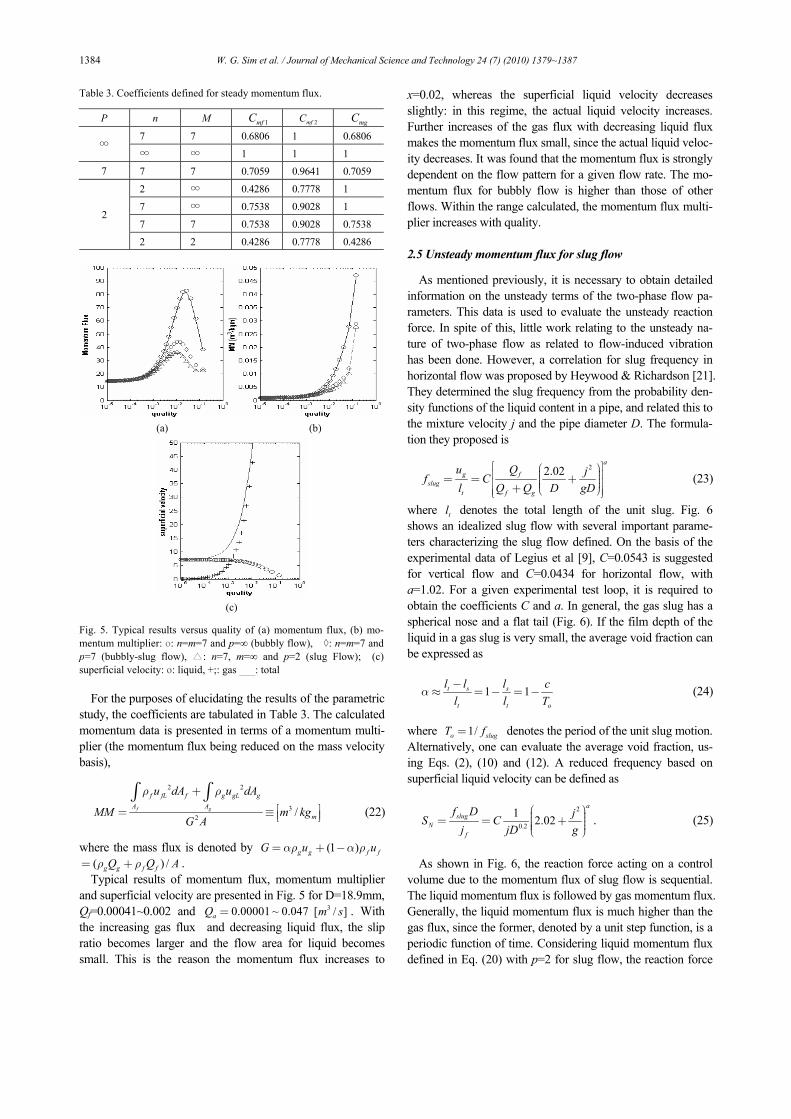
For the purposes of elucidating the results of the parametric study, the coefficients are tabulated in Table 3. The calculated momentum data is presented in terms of a momentum multi-plier (the momentum flux being reduced on the mass velocity basis),

2 2

32 /f g

f fL f g gL gA A

m

u dA u dA

MM m kgG A

ρ ρ+⎡ ⎤= ≡ ⎢ ⎥⎣ ⎦

∫ ∫ (22)

where the mass flux is denoted by (1 )g g f fG u uαρ α ρ= + −

( ) /g g f fQ Q Aρ ρ= + . Typical results of momentum flux, momentum multiplier

and superficial velocity are presented in Fig. 5 for D=18.9mm, Qf=0.00041~0.002 and 0.00001 ~ 0.047aQ = 3[ / ]m s . With the increasing gas flux and decreasing liquid flux, the slip ratio becomes larger and the flow area for liquid becomes small. This is the reason the momentum flux increases to

x=0.02, whereas the superficial liquid velocity decreases slightly: in this regime, the actual liquid velocity increases. Further increases of the gas flux with decreasing liquid flux makes the momentum flux small, since the actual liquid veloc-ity decreases. It was found that the momentum flux is strongly dependent on the flow pattern for a given flow rate. The mo-mentum flux for bubbly flow is higher than those of other flows. Within the range calculated, the momentum flux multi-plier increases with quality.

2.5 Unsteady momentum flux for slug flow

As mentioned previously, it is necessary to obtain detailed information on the unsteady terms of the two-phase flow pa-rameters. This data is used to evaluate the unsteady reaction force. In spite of this, little work relating to the unsteady na-ture of two-phase flow as related to flow-induced vibration has been done. However, a correlation for slug frequency in horizontal flow was proposed by Heywood & Richardson [21]. They determined the slug frequency from the probability den-sity functions of the liquid content in a pipe, and related this to the mixture velocity j and the pipe diameter D. The formula-tion they proposed is

22.02a

g fslug

t f g

u Q jf Cl Q Q D gD

⎡ ⎤⎛ ⎞⎟⎜⎢ ⎥⎟= = +⎜ ⎟⎢ ⎥⎜ ⎟⎜+ ⎝ ⎠⎢ ⎥⎣ ⎦ (23)

where tl denotes the total length of the unit slug. Fig. 6 shows an idealized slug flow with several important parame-ters characterizing the slug flow defined. On the basis of the experimental data of Legius et al [9], C=0.0543 is suggested for vertical flow and C=0.0434 for horizontal flow, with a=1.02. For a given experimental test loop, it is required to obtain the coefficients C and a. In general, the gas slug has a spherical nose and a flat tail (Fig. 6). If the film depth of the liquid in a gas slug is very small, the average void fraction can be expressed as

1 1t s s

t t o

l l l cl l T

α −≈ = − = − (24)

where 1/o slugT f= denotes the period of the unit slug motion. Alternatively, one can evaluate the average void fraction, us-ing Eqs. (2), (10) and (12). A reduced frequency based on superficial liquid velocity can be defined as

2

0.2

1 2.02a

slugN

f

f D jS Cj jD g

⎛ ⎞⎟⎜ ⎟= = +⎜ ⎟⎜ ⎟⎜⎝ ⎠. (25)

As shown in Fig. 6, the reaction force acting on a control

volume due to the momentum flux of slug flow is sequential. The liquid momentum flux is followed by gas momentum flux. Generally, the liquid momentum flux is much higher than the gas flux, since the former, denoted by a unit step function, is a periodic function of time. Considering liquid momentum flux defined in Eq. (20) with p=2 for slug flow, the reaction force

Table 3. Coefficients defined for steady momentum flux.

P n M 1mfC 2mfC mgC

7 7 0.6806 1 0.6806 ∞

∞ ∞ 1 1 1 7 7 7 0.7059 0.9641 0.7059

2 ∞ 0.4286 0.7778 1

7 ∞ 0.7538 0.9028 1

7 7 0.7538 0.9028 0.7538 2

2 2 0.4286 0.7778 0.4286

(a) (b)

(c)

Fig. 5. Typical results versus quality of (a) momentum flux, (b) mo-mentum multiplier: o: n=m=7 and p=∞ (bubbly flow), ◊: n=m=7 and p=7 (bubbly-slug flow), △: n=7, m=∞ and p=2 (slug Flow); (c) superficial velocity: o: liquid, +;: gas ___: total


given by liquid slugs can be formulated by the Fourier series

2(0 ) ( ) ( )2 2 2 2o o

l o f fLA

T c T cF t T u t u t u dAρ⎛ ⎞⎟⎜< < = − + − − − •⎟⎜ ⎟⎟⎜⎝ ⎠ ∫

2max

1

2 ( 1)(1 ) sin( (1 ))cos(2 )k

sfm f f slugk

K A u k k f tk

ρ α π α ππ

∞

=

⎛ ⎞− ⎟⎜ ⎟= − + −⎜ ⎟⎜ ⎟⎜⎝ ⎠∑

1

cos( )fo fk kk

A A tω∞

=

= +∑ (26)

where the coefficient for the unsteady momentum flux is de-fined as

2

2(1 / 2)(1 )sfmnK

n n=

+ + .

In the equation, the average void fraction for slug flow is ex-pressed in terms of c/To, as defined in Eq. (24). Similarly, one can express the force due to the gas flux (see Eq. (21) with n=2 and m=∞ ) by the Fourier series

2max

1

(0 )2 ( 1) sin( )cos(2 )

g ok

sgm g g slugk

F t T

K A u k k f tk

ρ α πα π ππ

∞

=

< <⎛ ⎞− ⎟⎜ ⎟= + +⎜ ⎟⎜ ⎟⎜⎝ ⎠∑

1

cos( )go gk kk

A A tω π∞

=

= + +∑ (27)

where 2

2(1 / 2)(1 )sgmmK

m m=

+ +.

The phase difference between the gas flux and the liquid flux is π, and the zero-order term of each momentum flux acts as a steady component. The coefficients defined for the un-

steady momentum flux of slug flow for various velocity dis-tributions are shown in Table 4. With the selected values n=7, m=∞ and p=2 for slug flow, the momentum fluxes, given by the gas and liquid of the slug flow, can be calculated by con-sidering Eqs. (20) and (21) for given mass fluxes of gas and liquid. The frequency of slug flow, fslug, was calculated by Eq. (23). Based on the Fourier series with the calculated momen-tum fluxes and the frequency, we can calculate the periodic reaction force. The periodic reaction forces and the major frequencies as defined by the Fourier series for momentum flux of slug flow are illustrated in Fig. 7. In the present results, the average void fraction was obtained by Eqs. (10) and (12). The first-order term was dominant.

In Fig. 8, a typical variation of the fundamental frequency and reduced frequency of momentum flux versus superficial liquid velocity, for k=1, is shown. The frequency varies ap-proximately linearly with superficial liquid velocity, as re-ported by Cheng et al. [19], Azzopardi & Baker [22] and Le-gius et al [9].

The root mean square of the periodic momentum flux of

Table 4. Coefficients defined for unsteady momentum flux of slug flow.

p n M sfmK sgmK

2 ∞ 0.3333 1

7 ∞ 0.6806 1

7 7 0.6806 0.6806 2

2 2 0.3333 0.3333

Fig. 6. Schematic diagram of slug flow and sequence of momentum flux by liquid and gas.

(a)

(b) Fig. 7. Periodic reaction forces and major frequencies as defined by Fourier series, for momentum flux of slug flow for n=7, m=∞ , p=2, β =0.75 and D=18.9 mm: (a) Qa=0.000421[m3/s], Qf=0.000140[m3/s];(b) Qa=0.000843[m3/s], Qf=0.000281[m3/s].

Fig. 8. Variation of fundamental frequency and reduced frequency, k=1, of momentum flux versus superficial liquid velocity for

0.0004aQ = 3[ / ]m s 0.00007 ~ 0.00182fQ = 3[ / ]m s and D= 18.9 mm.


slug flow is given by

max max

2 2 2 2

0

1 ( ) 1limT

RMS l g l gT o o

c cF F F dt F FT T T→∞

⎛ ⎞⎟⎜ ⎟= + = + −⎜ ⎟⎜ ⎟⎜⎝ ⎠∫

2 2 2 2max max(1 )( ) ( )sfm f f sgm g gK A u K A uα ρ α ρ= − + . (28)

Generally, the effect of gas flux on the value is minor. Thus,

the RMS value can be simplified as

2max (1 )RMS sfm f fF K A uρ α≈ − . (29)

The ratio of the simplified RMS flux to the steady compo-

nent (a zero-order term in Fourier series) depends only on the average void fraction; thus

2max

2max

(1 ) 1(1 ) 1

sfm f fRMS RMS

st fo sfm f f

K A uF FF A K A u

ρ αρ α α

−= = =

− −. (30)

The momentum multiplier can be expressed as

2 2

02

1 ( (1 ) )limT

g L gL f L fLATu u dAdt

TMM

G A

ρ α ρ α→∞

+ −=

∫ ∫, (31)

where G is the mass flux. Neglecting the effect of the gas term, which is very small compared with the liquid term, the multi-plier can be expressed in simple form by

2

2

1 2

1 1(1 )

sfm

f f f

KMM G A

C Cα

α ρ α

⎛ ⎞− ⎟⎜ ⎟⎜≈ ⎟⎜ ⎟⎜ ⎟− −⎝ ⎠. (32)

Various slug flow parameters for 0.00041 ~ 0.002fQ =

3[ / ],m s 30.00001 ~ 0.047[ / ]aQ m s= and 18.9D mm= are illustrated in Fig. 9. In the present results, a parabolic distribu-tion of the void fraction for the slug flow was used, p=2. It was found that the RMS value of the momentum flux given for the parabolic distribution of liquid velocity was larger than the others (n=7) and that the RMS values had peaks for which the real velocity of liquid was at the maximum. As expected, the effect of gas on the momentum flux was negligible. The data for the ratio of the RMS value to the static component versus the void fraction were collapsed, whereas the unsteady momentum multiplier for n=2 was larger than those of the others (n=7).

3. Conclusions

An analytical model for two-phase flow in a pipe was de-veloped based on a power law for the distributions of flow parameters such as gas velocity, liquid velocity and void frac-tion across the pipe diameter. Based on the power law, the average values of the parameters were calculated by integrat-ing the local parameters across the pipe area. The proposed integral analysis has several advantages over existing empiri-cal models. The integral forms can easily be incorporated into models for the determination of momentum flux and eventu-ally flow-induced forces in flow-structure interactions. A pa-rametric study with various distributions was performed for the average values of momentum flux and slip ratio, among others. Notably, the unsteady momentum flux for slug flow was approximated. The present void fraction and slip ratio results were compared with the existing empirical results, and a good agreement was revealed. It was found that the effect of liquid on the momentum flux is important, and that the latter is strongly dependent on the flow pattern for a given flow rate. The present formulations will be useful for laboratory calcula-

(a) (b) (c) (d) Fig. 9. Present results for slug flow with D=18.9mm, and Qa=0.00001~0.047[m3/s]: (a) RMS value of momentum flux; (b) ratio of RMS value to static component; (c) momentum multiplier for o: n=7, m= ∞ and p=2, : n=2, m=∞ and p=2, x: n=m=7 and p=2; (d) real (symbols) and superficial(lines) velocities, o --: liquid velocities, __: gas velocities, -.-.-: total superficial velocity.


tions of the average values of two-phase parameters through measurement of the maximum values at the center and the distributions. It would be desirable to verify the present model with experimental results and to examine the constants de-fined for the slug frequency. In a future study, the flow-induced vibration problem will be solved by applying an ex-citing force of known magnitude and frequency to a model of the system being studied.

4BReferences

[1] L. N. Carlucci, Damping and hydrodynamic mass of a cylin-der in simulated two-phase flow, Journal of Mechanical De-sign, 102 (1980) 597-602.

[2] L. N. Carlucci and J. D. Brown, Experimental studies of damping and hydrodynamic mass of a cylinder in confined two-phase flow”, Journal of Vibration, Acoustics, Stress, and Reliability in Design, 105 (1983) 83-89.

[3] M. J. Pettigrew, C. E. Taylor and B. S. Kim, Vibration of tube bundles in two-phase cross flow: Part 1 – hydrody-namic mass and damping, ASME Journal of Pressure Vessel Technology, 111 (1989) 466-477.

[4] M. J. Pettigrew, J. H. Tromp, C. E. Taylor, and B. S. Kim, Vibration of tube bundles in two phase cross flow: Part 2 – fluid-elastic instability, ASME Journal of Pressure Vessel Technology, 111 (1989) 478-487.

[5] M. J. Pettigrew and C. E. Taylor, Fluidelastic instability of heat exchanger tube bundles: review and design recommen-dations, ASME Journal of Pressure Vessel Technology, 113 (1991) 242-256.

[6] R. Fritz, The effect of liquids on the dynamic motions of immersed solids, ASME Journal of Engineering for Industry, 94 (1972) 167-173.

[7] S. J. Price, 1995, A review of theoretical models for flu-idelastic instability of cylinder arrays in cross-flow, Journal of Fluids and Structure, 9 (1995) 463-518.

[8] Jones, Jr. and N. Zuber, The interrelation between void frac-tion fluctuations and flow patterns in two-phase flow, Inter-national Journal of Multiphase Flow, 2 (1975) 273-306.

[9] H. J. W. M. Legius, H. E. A. van den Akker, and T. Narumo, Measurements on wave propagation and bubble and slug ve-locities in cocurrent upward two-phase Flow, Experimental Thermal and Fluid Science, 15 (1997) 267-278.

[10] W.-G. Sim, Stratified steady and unsteady two-phase flows between two parallel plates, Journal of Mechanical Science and Technology, 20 (1) (2006) 125-132.

[11] R. W. Lockhart, and R. C. Martinelli, Proposed correlation of data for isothermal two-phase, two-component flow in pipes, Chemical Engineering Progress, 45 (1949) 39-48.

[12] C. J. Baroczy, Correlation of liquid fraction in two-phase

with application to liquid metals, NAA-SR-8171 (1963). [13] J. M. Turner and G. B. Wallis, The separated-cylinders

model of two-phase flow, NYO-3114-6, Thayer’s School Eng., Dartmouth College, (1965).

[14] D. Butterworth, A comparison of some void-fraction rela-tionships for co-current gas-liquid flow, International Jour-nal of Multiphase Flow, 1 (1975) 845-850.

[15] N. Zuber and J. Findlay, Average volumetric concentration in two-phase flow system, Trans. ASME Journal of Heat Transfer, 11 (1965) 453-468.

[16] M. Ishii, T. C. Chawla and N. Zuber, Constitutive equation for vapor drift velocity in two-phase annular flow, AIChE, 22 (2) (1976) 283-289.

[17] N. Zuber, F. W. Staub, G. Bijwaard and P. G. Kroeger, Steady state and transient void fraction in two-phase flow system, GEAP 5471, (1967).

[18] G. B. Wallis, One-dimensional two-phase Flow, McGraw-Hill (1969).

[19] H. Cheng, J. H. Hills and B. J. Azzorpardi, A study of the bubble-to-slug transition in vertical gas-liquid flow in col-umns of different diameter, International Journal of Multi-phase Flow, 24 (1998) 431-452.

[20] Serizawa, I. Kataoka and I. Michiyoshi, Turbulence of air-water bubbly flow - II. Local properties, International Jour-nal of Multiphase Flow, 2 (1975) 235-246.

[21] N. I. Heywood and J. F. Richardson, Slug flow of air-water mixtures in a horizontal pipe: Determination of liquid holdup by γ -ray absorption, Chemical Engineering Science, 34 (1979) 17-30.

[22] B. J. Azzopardi and G. Baker, Characteristics of periodic structures in gas/liquid two-phase flow, UK/Japan Two-Phase Flow Meeting, Guildford, (2003).

[23] G. B. Andeen, P. Griffith, Momentum flux in two-phase flow, Journal of Heat Transfer, 90 (2) (1968) 211-222.

[24] D. S. Schrage, J. T. Hsu and M. K. Jensen, Two-phase pressure drop in vertical cross flow across a horizontal tube bundle, AIChE J, 34 (1988) 107-115.

Woo-Gun Sim received his B.S. degree in Mechanical Engineering from Inha University, Korea, in 1982. He was awarded his M.S. and Ph.D. degrees from McGill University, Canada, in 1987 and 1992, respectively. Dr. Sim is currently a Professor at the School of Mechanical Engineering at Hannam

University in Taejeon, Korea. Dr. Sim’s research interests include flow-induced vibration, two-phase flow and fluid dy-namics.

parametric study of two-phase flow by integral analysis

Documents