Scientia Iranica B (2015) 22(1), 235{244

Sharif University of TechnologyScientia Iranica

Transactions B: Mechanical Engineeringwww.scientiairanica.com

Parametric study of the pressure distribution in acon�ned aquifer employed for seasonal thermal energystorage

H. Ghaebi, M.N. Bahadori� and M.H. Saidi

Center of Excellence in Energy Conversion (CEEC), School of Mechanical Engineering, Sharif University of Technology, Tehran,P.O. Box 11155-9567, Iran.

Received 28 November 2013; received in revised form 28 February 2014; accepted 20 April 2014

KEYWORDSAquifer;Pressure distribution;Numerical simulation;Parametric study.

Abstract. Aquifers are underground porous formations containing water. Con�nedaquifers are formations surrounded by two impermeable layers. These aquifers are suitablefor seasonal thermal energy storage. The objective of this research is a parametric studyof the pressure distribution in an aquifer to be employed for thermal energy storage forair-conditioning of a building complex. In design of an Aquifer Thermal Energy Storage(ATES), a realistic model is needed to predict the aquifer's behavior. Here, the e�ects ofoperating parameters on pressure distribution are investigated through a three-dimensional�nite di�erence model. In an ATES, heat transfer occurs through both convection andconduction. The convective heat transfer in ATES occurs because of pressure gradient.Therefore, knowledge of the e�ects of various parameters on pressure distribution isnecessary. These parameters are: groundwater natural ow, the porosity and permeabilityof the aquifer, injection and withdrawal rates from wells, the number and the arrangements(being linear, triangular or rectangular) of injection and withdrawal wells. It has been foundthat variation of the pressure drop inside an aquifer with increasing permeability is veryconsiderable in comparison with other parameters. Moreover, a validation is performed byusing uent software to verify the accuracy of the developed method.© 2015 Sharif University of Technology. All rights reserved.

1. Introduction

Several countries, such as the United States [1-4], Eu-rope [5-9], and other countries [10,11], have employedcon�ned aquifers for the seasonal storage of thermal en-ergy for the heating and cooling of buildings. Recently,Seasonal Thermal Energy Storage (STES) systemshave become more popular in the world due to theproblems caused by the depletion of fossil fuels and theincrease of global warming [12]. The STES systems aregenerally divided into a closed system (e.g., BoreholeThermal Energy Storage, BTES), and an open system

*. Corresponding author. Tel./Fax: +98 21 66165583E-mail address: bahadori@sharif.edu (M.N. Bahadori)

(e.g., Aquifer Thermal Energy Storage, ATES). Due toits relatively high volumetric heat capacity, ATES hasa higher system performance than the BTES and othersystems employing low temperature geothermal heat.

Numerical modeling is a powerful tool for owsimulation in porous media such as an aquifer [13].In the past few years, several investigations have beenperformed into numerical simulation of ow in aquifers.They have also applied some numerical codes, suchas TRUST [14], TRUMP [15], PORFLOW [16], UN-SAT [17], SUTRA [18], and MODFLOW [19], to modelthe aquifer system. These codes are generally based on�nite di�erence discretization, and are used for owand temperature distribution inside the aquifer.

Tang and Jiao [20,21] derived a two-dimensional

236 H. Ghaebi et al./Scientia Iranica, Transactions B: Mechanical Engineering 22 (2015) 235{244

analytical solution to describe the groundwater uc-tuations in a leaky con�ned aquifer system near opentidal water. They assumed that the groundwater headin the con�ned aquifer uctuates in response to the seatide. They concluded that the groundwater responsein coastal areas depends not only on the aquiferproperties and structures, but also on the wave pattern.Aghbologhi et al. [22] developed a new analyticalsolution to describe the groundwater uctuation in asloping coastal aquifer system comprised of an upperuncon�ned aquifer, a lower con�ned aquifer, and anaquitard in between. The research results indicatedthat the e�ect of the bottom angle on groundwater uctuation and time lag is signi�cant in the uncon�nedaquifer and not negligible if the leakage in the con�nedaquifer is large. Kihm et al. [23] performed a series ofthree-dimensional numerical simulations using a hydro-geo-mechanical numerical model to analyze and predictfully coupled groundwater ow and land deformationdue to groundwater pumping in an unsaturated uvialaquifer system, which has irregular lateral boundaries.They used the �nite element method for the analyses.

These numerical simulation results show thathydro-geo-mechanical numerical modeling can be a use-ful tool for analyzing and predicting long-term ground-water level uctuations and land deformation dueto groundwater pumping in actual three-dimensionalaquifer systems. Shuang et al. [24] conducted a seriesof numerical simulations to investigate the e�ect of theslope of the outlet-capping on the tide-induced head uctuations in a coastal con�ned aquifer. The nu-merical simulations demonstrated that when hydraulicdi�usivity, slope and/or the outlet-capping leakagesare large, tidal loading e�ect is relatively weak andleakage dominates. Ayvaz and Karahan [25] intro-duced a Simulation/Optimization (S/O) model for theidenti�cation of unknown groundwater well locationsand pumping rates for two-dimensional aquifer sys-tems. The proposed S/O model uses a �nite-di�erencesolution of the governing groundwater ow equation asits simulation model. This model is then combinedwith a Genetic Algorithm (GA) based optimizationmodel which is used to determine the pumping ratesfor each well. The performance of the proposed S/Omodel is tested on two hypothetical aquifer modelsfor both steady-state and transient ow conditions.Laplace domain solutions have been obtained for three-dimensional groundwater ow to a well in con�nedand uncon�ned wedge-shaped aquifers by Sedighi etal. [26]. The solutions take into account partialpenetration e�ects, instantaneous drainage or delayedyield, vertical anisotropy and water table boundarycondition. The results are presented in the form ofdimensionless drawdown-time and boundary gradient-time type curves. Nam and Ooka [27] investigatedapplication of a Groundwater Heat Pump (GWHP)

system in an open-loop system that draws water from awell or surface water for heating/cooling of a building.In their research, 3D numerical heat transfer simulationand experiments, utilizing real-scale equipment, wasconducted using a numerical code, named EFLOW, inorder to develop the optimization method for GWHPsystems. Simulation results were compared with theexperimental ones, and the validity of the simulationmodel was con�rmed. Dafny et al. [28] studied thein uences of the geological structure (especially foldingand lithology) and the karst system on the ground-water ow regime. They introduced a 3D geological-based grid for the basin for the �rst time. It wasimplemented into FEFLOW, which was used, there-after, to analyze, quantitatively, the ow regime, thegroundwater mass balance, and the aquifer hydraulicproperties. Modeling results have also exhibited thatin the lowland con�ned area, the geological structuredoes not play a major role in directing groundwater ow. Sensitivity analysis of a steady-state groundwater ow equation of the ow parameters and the boundaryconditions, based on the perturbation approach, hasbeen performed by Mazzilli et al. [29]. Recently,Hu et al. [30] developed a numerical model basedon the Galerkin �nite element method and the �nitedi�erence method for a homogeneous and isotropiccon�ned aquifer in which a pumping well penetratesa di�erent thickness of aquifer, and a number of fullpenetrating observation boreholes are placed to obtaindrawdowns. They selected a hypothetical example tojustify the extent and magnitude of the in uences,and to demonstrate the e�ect of well diameter on the ow within an observation well. Their study suggeststhat one must be cautious in using hydraulic headsfrom observation wells to evaluate groundwater owsystems before the pipe- ow e�ect can be assumedto be negligible. Velazquez et al. [31] presented aconceptual-numerical model that can be deduced froma calibrated �nite di�erence groundwater ow modelfor investigation into the response of the aquifer headdistribution to surface water. Their results showedthat penetration of water from the surface into theaquifer modi�ed the pressure distribution inside theaquifer. Rushton and Brassington [32] consideredthe signi�cance of the hydraulic head distribution forhorizontal wells in shallow aquifers, and estimatedthe in ows of groundwater along the length of thewell. After conceptual and computational modeling,they deduced that there are signi�cant drawdowns ingroundwater heads in the vicinity of the well. Yeh andChang [33] summarized recent developments of owmodeling, such as the ow in aquifers, with horizontalwells or collector wells, capture zone delineation, andnon-Darcian ow in porous media and fractured for-mations. They also presented a comprehensive reviewon the numerical calculations for �ve well functions

H. Ghaebi et al./Scientia Iranica, Transactions B: Mechanical Engineering 22 (2015) 235{244 237

frequently appearing in well-hydraulic literature, andsuggested some topics in groundwater ow for futureresearch. Marion et al. [34] simulated a sharp interfacemodel issuing from a seawater intrusion problem in afree aquifer. They also modeled the evolution of thesea front and of the upper free surface of the aquifer.They used a P1 �nite element method for the spacediscretization combined with a semi-implicit in-timescheme.

The sub-objectives of this research paper aremultiple, and include:

� Carrying out a numerical modeling for pressuredistribution in an aquifer used for thermal energystorage.

� Comprehensively investigating the in uence of vari-ous hydro-geological and operational parameters onpressure distribution inside an aquifer.

� Examining the use of various numbers and arrange-ments for injection and withdrawal wells.

� Investigating the e�ect of well layout on pressuredistribution in the aquifer.

2. System description

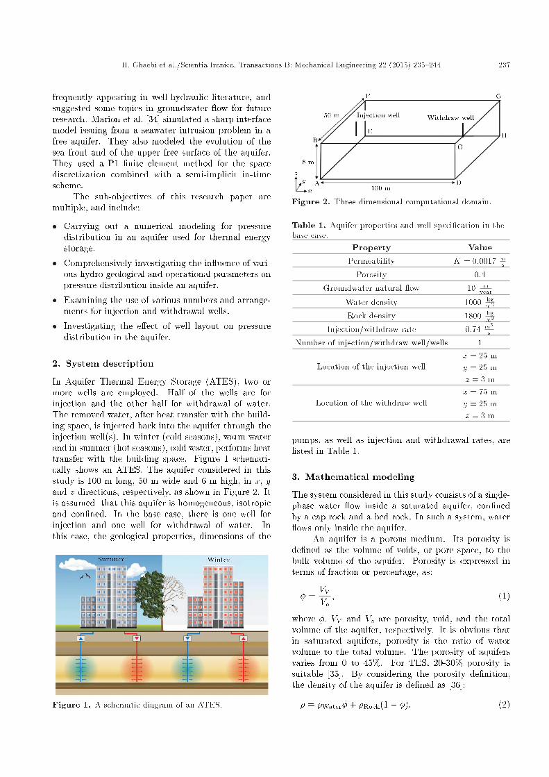
In Aquifer Thermal Energy Storage (ATES), two ormore wells are employed. Half of the wells are forinjection and the other half for withdrawal of water.The removed water, after heat transfer with the build-ing space, is injected back into the aquifer through theinjection well(s). In winter (cold seasons), warm waterand in summer (hot seasons), cold water, performs heattransfer with the building space. Figure 1 schemati-cally shows an ATES. The aquifer considered in thisstudy is 100 m long, 50 m wide and 6 m high, in x, yand z directions, respectively, as shown in Figure 2. Itis assumed that this aquifer is homogeneous, isotropicand con�ned. In the base case, there is one well forinjection and one well for withdrawal of water. Inthis case, the geological properties, dimensions of the

Figure 1. A schematic diagram of an ATES.

Figure 2. Three dimensional computational domain.

Table 1. Aquifer properties and well speci�cation in thebase case.

Property Value

Permeability K = 0:0017 ms

Porosity 0.4

Groundwater natural ow 10 myear

Water density 1000 kgm3

Rock density 1800 kgm3

Injection/withdraw rate 0:74 m3

s

Number of injection/withdraw well/wells 1

Location of the injection wellx = 25 my = 25 mz = 3 m

Location of the withdraw wellx = 75 my = 25 mz = 3 m

pumps, as well as injection and withdrawal rates, arelisted in Table 1.

3. Mathematical modeling

The system considered in this study consists of a single-phase water ow inside a saturated aquifer, con�nedby a cap rock and a bed rock. In such a system, water ows only inside the aquifer.

An aquifer is a porous medium. Its porosity isde�ned as the volume of voids, or pore space, to thebulk volume of the aquifer. Porosity is expressed interms of fraction or percentage, as:

� =VVVo; (1)

where �, VV and Vo are porosity, void, and the totalvolume of the aquifer, respectively. It is obvious thatin saturated aquifers, porosity is the ratio of watervolume to the total volume. The porosity of aquifersvaries from 0 to 45%. For TES, 20-30% porosity issuitable [35]. By considering the porosity de�nition,the density of the aquifer is de�ned as [36]:

� = �Water�+ �Rock(1� �): (2)

238 H. Ghaebi et al./Scientia Iranica, Transactions B: Mechanical Engineering 22 (2015) 235{244

Water ow is a function of the pressure distributionin the aquifer and its physical properties. In general, ow is proportional to the pressure gradient or headgradient, and the area [37]:

Q _ AdhdL

: (3)

This ow relationship is known as Darcy's law, and itsproportionality is called permeability:

Q = �KAdhdL

: (4)

The minus sign is necessary, because the head decreasesin the direction of the ow. Another form of Darcy'slaw is written for the Darcy ux (or Darcy velocity, orspeci�c velocity), which is the discharge rate per unitcross-sectional area. It is generally hard to de�ne thevelocity in an aquifer because of the existence of poreswith di�erent cross sections. The velocity in the aquifermust be a rough average number, as the cross sectionis never homogeneous. As a result, velocity is rarelyused in geological evaluations. A velocity de�ned bydividing the ow rate (Q) by the aquifer cross-sectionalarea (A) is known as the speci�c velocity or VS [37]:

~VS =QA

= �K dhdL

: (5)

Natural ow in an aquifer is accounted for in theequations of ow. The natural ow in an aquifer canbe stated as:

Q=A = K~�h: (6)

Practically, groundwater ows in a complex 3D pat-tern. Darcy's law in three dimensions is analogous tothat of one dimension. In a Cartesian x, y, z coordinatesystem, it is commonly expressed as:

~VS;x = �Kx@h@x; (7)

~VS;y = �Ky@h@y; (8)

~VS;z = �Kz@h@z; (9)

where Kx, Ky and Kz are the hydraulic conductivity inthree coordinate directions of x, y and z, respectively.In general, for a given porous medium, Kx , Ky and Kzdo not need to be the same in which case, the mediumis called anisotropic. On the other hand, if Kx = Ky =Kz, the medium is called isotropic. In this study, weassume that the aquifer is isotropic.

For most natural ows, the head (h) gradientis gradual and the ow rate can be estimated read-ily. Natural ow rates normally vary between 1.5 to

100 myear . To consider an aquifer for TES, the ow rates

should be 10 myear , or less [36].

The general form of the Darcy equation can bewritten in such a way that the e�ect of the gravity istaken into account [38]:

~VS = �k�

�~�h� �~g� ; (10)

where ~VS , k and � are speci�c velocity, speci�c per-meability and viscosity, respectively, and h, � and ~gare pressure head, aquifer density and gravitationalacceleration, respectively.

In ATES, charge and discharge ows are gener-ally performed at constant rates in the operationalperiod. Therefore, the ow is steady and the contin-uum equation in porous media satis�es the followingequation [39]:h

~�:(�~VS)idV = S: (11)

S is related to the source term, and it is the rate ofinjection/withdrawal. In this study, it is supposed thatthe porosity and density are constant, hence, Eq. (11)is rewritten as:

~�:~VS =S (x; y; z)�dV

: (12)

By considering Darcy's equation, ~VS = Krh, Eq. (12)can be stated as follows:

�2h =S (x; y; z)K�dV

: (13)

4. Numerical simulation

Numerical simulations of problems in uid dynamicsare usually formulated using one of three methods:�nite element, �nite volume and �nite di�erence [40].In the �nite di�erence approach, a �nite di�erenceapproximation of the di�erential equation is solved.When this numerical method is applied, the equation is�rst transformed from the physical domain to a uniformcomputational domain, and the di�erential form of theequation is usually solved at the node points.

In this research, the �nite di�erence approach wasused for modeling the ow domain in a con�ned aquifer.The computational domain was three dimensional.Using the �nite di�erence approach is conventional inATES ow and thermal modeling. Since the boundarycondition in an aquifer is simple, using the uniformstructured mesh is more applicable.

The �rst step in a �nite di�erence scheme isdiscretization. For this purpose, Eq. (13) is writtenas follows:

@2h@x2 +

@2h@y2 +

@2h@z2 =

S (x; y; z)K�dV

: (14)

H. Ghaebi et al./Scientia Iranica, Transactions B: Mechanical Engineering 22 (2015) 235{244 239

Figure 3. Meshing view.

The above equation was solved numerically using thefractional steps method in three dimensions. Initially,the equation was solved using the Crank-Nicolson im-plicit method, and results of the solution in one direc-tion (for example, x direction) were used for solution inother directions (y and z directions). In any direction,the solution was performed by applying Thomas'sTDMA (Three Diagonal Matrix Algorithm). A centraldi�erence scheme is used to discretize Eq. (14).

It should be noted that this method has a secondorder truncation error in each direction. The advantageof this procedure is its unconditional stability andhigher rate of convergence, because of using the TDMAmethod. The more detailed discretization process ispresented in Appendix A.

Meshing was performed in such a way that in-jection/withdrawal wells were considered in any nodeof the computational domain. Figure 3 shows themeshing arrangement. For investigation of mesh sizeindependency, so that the unique solution would beobtained, several mesh sizes were examined. Finally,the mesh sizes selected were 1 m, 1 m and 0.5 m, inx, y and z directions, respectively. The dependency ofthe solution on mesh sizes less than these values wasless than 1 percent. In this structured meshing, thenumber of meshes was about 67000.

To start up the solution, boundary conditions inx, y and z directions were applied. In ABFE andDCGH planes, shown in Figure 2, a pressure gradientwas inserted, while the ground water ow was in the x-direction. This value of pressure gradient was obtainedfrom Darcy's equation as follows:Himp = VgwXlength=K: (15)

The boundary conditions in ABFE and DCGH planeswere as follows:h1;j;k = Himp; hN;j;k = 0: (16)

The boundary conditions in lateral faces of ABCD andEFGH and top and bottom faces of AEHD and BFGCfaces were no-penetration boundary conditions.

5. Discussion and results

Initially, the pressure distribution was calculated forthe base case design. The properties of the aquifer and

the locations of the injection and withdrawal wells arespeci�ed in Table 1.

In the following discussion, the pressure distri-bution was calculated in three dimensions. However,because of the symmetry of the domain, the pressuredistribution is shown only in x direction, y = 25 mand z = 3 m. A zero pressure was arbitrarily assumedat x = 75 m, where water is entering the withdrawalwell.

5.1. Model veri�cationTo investigate the accuracy of the developed code,a validation was performed using FLUENT softwareand simulation of the computational domain. Thecomputational domain is shown in Figure 4. In thismeshing, an unstructured 3D mesh of 259346 cellswas built. The chosen element was Tet/Hybrid andthe type was TGrid. For veri�cation, the head wascompared with that obtained via the developed code(Table 2) between the well pairs in an x direction, aty = 25 m and z = 3 m, for the base case. The resultsshow a good correspondence between the developedcode and those obtained using FLUENT.

Figure 4. Model mesh in FLUENT.

Table 2. Model veri�cation with results of FLUENTsimulation.

x (m)Head (m)

HFLUENT HCode Error (%)

25 14.24 13.56 4.77

30 8.26 7.72 6.53

35 7.82 7.52 3.83

40 7.55 7.14 5.43

45 7.32 6.94 5.19

50 7.08 6.83 3.53

55 6.91 6.68 3.32

60 6.69 6.47 3.28

65 6.41 6.23 2.80

70 5.98 5.86 2.01

240 H. Ghaebi et al./Scientia Iranica, Transactions B: Mechanical Engineering 22 (2015) 235{244

Table 3. E�ect of the variation of the groundwatervelocity on the pressure distribution.

Groundwater velocity(m/year)

Maximum pressure inthe aquifer (m)

10 14.1599

30 14.2065

50 14.2251

100 14.2438

5.2. The e�ect of groundwater natural ow onthe pressure distribution between wellpairs

Variation of groundwater velocity has a very lowe�ect on the pressure distribution between well pairs.Table 3 shows the maximum pressure between wellpairs (at the location of the injection well) for di�erentgroundwater velocities. Since the natural groundwater ow is considered in the x direction, the natural owis in uenced by the pressure distribution in the bound-aries and in planes perpendicular to the x direction.By increasing groundwater velocity, the maximumpressure in the aquifer (at the location of the injectionwell) is increased (Eqs. (10), (15) and (16)) slightly,and, consequently, pressure loss between well pairs isincreased as well.

5.3. The e�ect of porosity on the pressuredistribution between well pairs

Figure 5 shows the pressure distribution between wellpairs, with respect to porosity. As seen, by increasingthe porosity, the pressure losses are increased. Thishappens because the increment in porosity tends toincrease the void space inside the aquifer and the higher ow rate between wells.

5.4. The e�ect of permeability on the pressuredistribution between well pairs

Hydraulic conductivity (permeability) is the abilityof porous media to transmit water. It should be

Figure 5. Variation of pressure distribution between wellpairs with porosity at y = 25 and z = 3 m, and forK = 0:0017 m

s , Vgw = 10 myear and Q = 0:74 m3

s .

Figure 6. Variation of pressure distribution between wellpairs with permeability at y = 25 and z = 3 m, and for� = 0:4, Vgw = 10 m

year and Q = 0:74 m3

s .

noted that the hydraulic conductivity implies hydraulicresistance of an aquifer. Figure 6 shows the variationof pressure distribution, with respect to permeability.As permeability increases, the hydraulic resistance withrespect to ow is decreased. As a result, the pressureloss between wells is decreased. According to Eq. (10),lower ow occurs because of lower pressure di�erences.

5.5. The e�ect of injection/withdrawal rate onthe pressure distribution between wellpairs

Figure 7 shows the e�ects of injection/withdrawal rateson the pressure distribution. The injection/withdrawalrate is the source term in the pressure distributionequation. As shown in Eq. (14), by increasing owrate, pressure losses are increased. It should be notedthat in this research, the injection rate is the same asthe withdrawal rate.

5.6. The e�ect of number and arrangement ofwells on the pressure distribution betweenwell pairs

In the previous sections, one pair of injection/withdr-awal wells was used. An objective of this research was

Figure 7. Variation of pressure distribution between wellpairs with injection/withdrawal ow rate at y = 25 andz = 3 m, and for K = 0:0017 m

s , Vgw = 10 myear and � = 0:4.

H. Ghaebi et al./Scientia Iranica, Transactions B: Mechanical Engineering 22 (2015) 235{244 241

Figure 8. A three-well application: a) Lineararrangement; and b) triangular arrangement.

to investigate the e�ects of number and the arrange-ment of wells (being linear, triangular and rectangular)on pressure distribution inside the aquifer.

5.6.1. A three-well arrangementFigure 8 shows the dimensions and the arrangements ofthree wells employed for injection, and three wells usedfor the withdrawal of water. The arrangements can belinear or triangular, as shown in Figure 8(a) and (b),respectively.

Pressure distribution in the aquifer is shown inFigure 9 in a three-well application. As seen, pressurelosses in the linear array are more than in the triangulararrangement.

5.6.2. A �ve-well arrangementFigure 10 shows the arrangement of a �ve-well appli-cation. In this case, the array can be linear, triangularor rectangular, as shown in Figure 10(a), (b) and (c),respectively.

Figure 11 shows the pressure distribution in a �ve-well application. As seen, pressure losses in the lineararrangement are slightly higher.

6. Conclusion

A parametric study of pressure distribution in a con-�ned aquifer employed for seasonal thermal energystorage was carried out in this research. The e�ects of

Figure 9. Pressure distribution between well pairs in athree-well application for K = 0:0017 m

s , Vgw = 10 myear ,

� = 0:4 and Q = 0:74 m3

s .

Figure 10. A �ve-well application: a) Lineararrangement; b) triangular arrangement; and c)rectangular arrangement.

242 H. Ghaebi et al./Scientia Iranica, Transactions B: Mechanical Engineering 22 (2015) 235{244

Figure 11. Pressure distribution between well pairs in a�ve-well application for K = 0:0017 m

s , Vgw = 10 myear ,

� = 0:4, Q = 0:74 m3

s .

the groundwater natural ow, porosity, permeability,injection and withdraw rates, numbers and arrange-ments (linear, triangular and rectangular) of wells wereinvestigated. The following conclusions may be drawnfrom this research:

� By increasing the natural ow of ground water,pressure loss in the aquifer increases.

� An increase of porosity leads to lowering of thepressure loss.

� As permeability increases, the pressure loss in theaquifer decreases.

� As injection/withdraw rates increase, the pressureloss increases.

� When the number of wells increases, while thetotal injection/withdraw rates remain unchanged,the pressure loss increases.

� The pressure losses in the linear three-well and�ve-well arrangements are higher than when thearrangements are triangular and rectangular.

References

1. Meyer, C.F. and Todd, D.K. \Heat storage wells",Water Well Journal, 10, pp. 35-41 (1973).

2. Molz, F.J., Warman, J.C. and Jones, T.E. \Aquiferstorage of heated water: Part 1: A �eld experiment",Ground Water, 16, pp. 234-241 (1978).

3. Papadopulos, S.S. and Larson, S.P. \Aquifer storageof heated water: Part 2: Numerical simulation of �eldresults", Ground Water, 16, pp. 242-248 (1978).

4. Parr, D.A., Molz, F.J. and Melville, J.G. \Fielddetermination of aquifer thermal energy storage pa-rameters", Ground Water, 21, pp. 22-35 (1983).

5. Sanner, B., Karytsas, C., Mendrinos, D. and Rybach,L. \Current status of ground source heat pumps

and underground thermal energy storage in Europe",Geothermics, 32, pp. 579-588 (2003)

6. Paksoy, H.O., Andersson, O., Abaci, S., Evliya, H. andTurgut, B. \Heating and cooling of a hospital usingsolar energy coupled with seasonal thermal energystorage in an aquifer", Renewable Energy, 19, pp. 117-122 (2000).

7. Dickinson, J.S., Buik, N., Matthews, M.C. and Sni-jders, A. \Aquifer thermal energy: Theoretical andoperational analysis", Geotechnique, 59, pp. 249-260(2009).

8. Novo, V.A., Bayon, R.J., Castro-Fresno, D. andRodriguez-Hernandez, R. \Review of seasonal heatstorage in large basins: Water tanks and gravel waterpits", Applied Energy, 87, pp. 390-397 (2010).

9. Preene, M. and Powrie, W. \Ground energy sys-tems: Delivering the potential", Energy, 34, pp. 77-84(2009).

10. Umemiya, H. and Satoh, Y. \A cogeneration systemfor a heavy-snow fall zone based on aquifer thermalenergy storage", Japanese Society of Mechanical Engi-neering, 33, pp. 757-765 (1990).

11. Lee, K.S. \Performance of open borehole thermal en-ergy storage system under cyclic ow regime", Journalof Geoscience, 12, pp. 169-175 (2008).

12. Rosen, M.A. \Second-law analysis of aquifer thermalenergy storage systems", Energy, 24, pp. 167-182(1999).

13. Shamsai, A. and Vosoughifar, H.R. \Finite volumediscretization of ow in porous media by MATLABsystem", Scientia Iranica, 11, pp. 146-153 (2004).

14. Narasimhan, T.N. \TRUST: A computer programfor transient and steady state uid ow in multi-dimensional variably saturated deformable media un-der isotherm conditions", Lawrence Berkeley Labora-tory Memorandum (1984).

15. Schauer, D.A. \FED: A computer program to generategeometric input for the heat transfer code TRUMP",Report UCRL-50816 (1973).

16. Runchal, A.K. \PORFLOW: A software tool for multiphase uid ow, heat and mass transport in fracturedporous media, user's manual version 2.50", Analytical& Computational Research, Inc., Los Angeles, CA90077 (1984).

17. Fayer, M. and Jones, T. \UNSAT-H version 2.0: Un-saturated soil water and heat ow model", PNL-6779,Paci�c Northwest Laboratory, Richland, Washington(1990).

18. Souza, W.R. \Documentation of a graphical displayprogram for the saturated-unsaturated transport (SU-TRA) �nite element simulation model", U.S. Geo-logical Survey Water-Resource Investigation Report874245 (1987).

19. Jobson, H.E. and Harbaugh, A.W. \Modi�cations tothe di�usion analogy surface-water ow model (da ow)

H. Ghaebi et al./Scientia Iranica, Transactions B: Mechanical Engineering 22 (2015) 235{244 243

for coupling to the modular �nite-di�erence ground-water ow model (Mod ow)", U.S. Geological SurveyOpen-File Report 99-217 (1999).

20. Tang, Z. and Jiao, J.J. \A two-dimensional analyticalsolution for groundwater ow in a leaky con�nedaquifer system near open tidal water", HydrologicalProcesses, 15, pp. 573-585 (2001).

21. Jiao, J.J. and Tang, Z. \An analytical solution ofgroundwater response to tidal uctuation in a leakycon�ned aquifer", Water Resources Research, 35, pp.747-751 (1999).

22. Aghbolaghi, M.A., Chuang, M.H. and Yeh, H.D.\Groundwater response to tidal uctuation in a slopingleaky aquifer system", Applied Mathematical Mod-elling, 36, pp. 4750-4759 (2012).

23. Kihm, J.H., Kim, J.M., Sung-Ho, S. and Gyu-Sang,L. \Three-dimensional numerical simulation of fullycoupled groundwater ow and land deformation due togroundwater pumping in an unsaturated uvial aquifersystem", Journal of Hydrology, 35, pp. 1-14 (2007).

24. Shuang, L., Hailong, L., Boufadel, M.C. and Guohui,L. \Numerical simulation of the e�ect of the slopingsubmarine outlet-capping on tidal groundwater head uctuation in con�ned coastal aquifers", Journal ofHydrology, 36, pp. 339-348 (2008).

25. Ayvaz, M.T. and Karahan, H. \A simulation/ op-timization model for the identi�cation of unknowngroundwater well locations and pumping rates", Jour-nal of Hydrology, 35, pp.76-92 (2008).

26. Sedghi, M.M., Samani, N. and Sleep, B. \Three-dimensional semi-analytical solution to groundwa-ter ow in con�ned and uncon�ned wedge-shapedaquifers", Advances in Water Resources, 32, pp. 925-935 (2009).

27. Nam, Y. and Ooka, R. \Numerical simulation ofground heat and water transfer for groundwater heatpump system based on real-scale experiment", Energyand Buildings, 42, pp. 69-75 (2010).

28. Dafny, E., Burg, A. and Gvirtzman, H. \E�ects ofkarst and geological structure on groundwater ow:The case of Yarqon-Taninim aquifer, Israel", Journalof Hydrology, 38, pp. 260-275 (2010).

29. Mazzilli, N., Guinot, V. and Jourde, H. \Sensitivityanalysis of two-dimensional steady-state aquifer owequations. Implications for groundwater ow modelcalibration and validation", Advances in Water Re-sources, 33, pp. 905-922 (2010).

30. Hu, L., Chen, C. and Chen, X. \Simulation ofgroundwater ow within observation boreholes forcon�ned aquifers", Journal of Hydrology, 39, pp. 101-108 (2011).

31. Velazquez, D.P., Sahuquillo, A. and Andreu, J.\A conceptual-numerical model to simulate hydraulichead in aquifers that are hydraulically connected to

surface water bodies", Hydrological Process, 25, DOI:10.1002/hyp.8214 (2011).

32. Rushton, K.R. and Brassington, F.C. \Signi�cance ofhydraulic head gradients within horizontal wells inuncon�ned aquifers of limited saturated thickness",Journal of Hydrology, 49, pp. 281-289 (2013).

33. Yeh, H.D. and Chang, Y.Ch. \Recent advances in mod-eling of well hydraulics", Advances in Water Resources,51, pp. 27-51 (2013).

34. Marion, P., Najib, K. and Rosier, C. \Numericalsimulations for a seawater intrusion problem in a freeaquifer", Applied Numerical Mathematics, 75, pp. 48-60 (2014).

35. Tsang, C.F., Aquifer Thermal Energy Storage, ASurvey, LBL Report, USA (1980).

36. Schaetzle, W.J., Thermal Energy Storage in Aquifers,Design and Applications, Pergamon Press, UK (1980).

37. Strack, O.D.L., Groundwater Mechanins, PrenticeHall, USA (1989).

38. Kangas, M.T. and Lund, P.D. \Comparison of longterm ATES experiment to 3-D computer simulation",Proceeding of 26th International Energy ConversionConference, Boston, MA, USA (1985).

39. Kangas, M.T. and Lund, P.D. \Modeling and simula-tion of aquifer storage energy system", Solar Energy,53, pp. 237-247 (1994).

40. Bear, J., Dynamic of Fluids in Porous Media, Elsevier,Dover Publication. Inc. publisher, pp. 450-510 (1992).

41. Ho�mann, K.A. and Chiang, S.T., ComputationalFluid Dynamic, Publication of Engineering educationSystem, USA (2000).

Appendix A

By de�ning the following parameters:

Ex =1

�x2 ; (A.1)

Ey =1

�y2 ; (A.2)

Ez =1

�z2 : (A.3)

Eq. (14) is discretized, as follows, in the functionalsteps method [41]:

Sweeping in x direction:�Ex2

�h�i+1;j;k � (Ex)h�i;j;k +

�Ex2

�h�i�1;j;k

=Si;j;kK�dV

��Ex2

�hni+1;j;k+(Ex+Ey+Ez)hni;j;k

244 H. Ghaebi et al./Scientia Iranica, Transactions B: Mechanical Engineering 22 (2015) 235{244

��Ex2

�hni�1;j;k�(Ey)hni;j+1;k � (Ey)hni;j�1;k

� (Ez)hni;j;k+1 � (Ez)hni;j;k�1: (A.4)

Sweeping in y direction:�Ey2

�h��i;j+1;k � (Ey)h��i;j;k +

�Ey2

�h��i;j�1;k

=Si;j;kK�adV

��Ex2

�h�i+1;j;k+(Ex)h�i;j;k

��Ex2

�h�i�1;j;k�

�Ex2

�hni+1;j;k

+ (Ex+Ey+Ez)hni;j;k ��Ex2

�hni�1;j;k

��Ey2

�hni;j+1;k �

�Ey2

�hni;j�1;k

� (Ez)hni;j;k+1 � (Ez)hni;j;k�1: (A.5)

Sweeping in z direction:�Ez2

�hn+1i;j;k+1 � (Ez)hn+1

i;j;k +�Ez2

�hn+1i;j;k�1

=Si;j;kK�dV

��Ex2

�h�i+1;j;k+(Ex)h�i;j;k

��Ex2

�h�i�1;j;k�

�Ex2

�hni+1;j;k

+ (Ex+Ey+Ez)hni;j;k ��Ex2

�hni�1;j;k

��Ey2

�h��i;j+1;k + (Ey)h��i;j;k

��Ey2

�h��i;j�1;k �

�Ey2

�hni;j+1;k

��Ey2

�hni;j�1;k �

�Ez2

�hni;j;k+1

��Ez2

�hni;j;k�1: (A.6)

It should be noted that n and n+ 1 are related to twosuccessive iterations.

Biographies

Hadi Ghaebi is currently a PhD degree student atSharif University of Technology, Tehran, Iran. Hisresearch areas include thermal system design andoptimization, renewable energy technologies, net zeroenergy buildings and hydrogen and fuel cells.

Mehdi Bahadorinejad received his PhD degree inMechanical Engineering from the University of Illi-nois, USA, in 1964, and is currently Professor ofMechanical Engineering at Sharif University of Tech-nology, Tehran, Iran. His research interests in-clude natural cooling systems, solar energy utilization,environmentally- compatible energy systems, develop-ment of indigenous technology, application of scienti�c-spiritual thinking to social problems, entropy andawareness and engineering ethics and engineering ofethics.

Mohammad Hassan Saidi is Professor in the Schoolof Mechanical Engineering at Sharif University of Tech-nology, Tehran, Iran. His current research interestsinclude MEMS, heat transfer enhancement in boilingand condensation, modeling of pulse tube refrigeration,vortex tube refrigerators, indoor air quality and cleanroom technology, energy e�ciency in home appliances,and desiccant cooling systems.