Parametric Solutions to the Generalized Fermat

Equation

27 April 2016

Advisor: Dr. Tom Fisher

1

Contents

1 Introduction 3

1.1 The Generalized Fermat Equation . . . . . . . . . . . . . . . . . . . . . . . . . . . . . . . . . 3

1.2 Outline of the Essay . . . . . . . . . . . . . . . . . . . . . . . . . . . . . . . . . . . . . . . . . 3

2 Invariant Theory and Klein Forms 4

2.1 Finite Rotation Groups . . . . . . . . . . . . . . . . . . . . . . . . . . . . . . . . . . . . . . . 4

2.2 Invariant Polynomials . . . . . . . . . . . . . . . . . . . . . . . . . . . . . . . . . . . . . . . . 5

2.3 Regular Plane Polygons . . . . . . . . . . . . . . . . . . . . . . . . . . . . . . . . . . . . . . . 6

2.4 Octahedron . . . . . . . . . . . . . . . . . . . . . . . . . . . . . . . . . . . . . . . . . . . . . . 7

2.5 Tetrahedron and Icosahedron . . . . . . . . . . . . . . . . . . . . . . . . . . . . . . . . . . . . 8

2.6 Klein Forms . . . . . . . . . . . . . . . . . . . . . . . . . . . . . . . . . . . . . . . . . . . . . . 8

3 Parametrized Solutions 10

3.1 Some Preliminaries . . . . . . . . . . . . . . . . . . . . . . . . . . . . . . . . . . . . . . . . . . 10

3.2 Proof of the Main Result . . . . . . . . . . . . . . . . . . . . . . . . . . . . . . . . . . . . . . 12

4 Constructing Explicit Solutions 15

4.1 Restricting to Klein Forms . . . . . . . . . . . . . . . . . . . . . . . . . . . . . . . . . . . . . . 15

4.2 Classification of Klein Forms . . . . . . . . . . . . . . . . . . . . . . . . . . . . . . . . . . . . 15

4.3 Lifting Integer Solutions . . . . . . . . . . . . . . . . . . . . . . . . . . . . . . . . . . . . . . . 16

4.4 Hermite Reduction Theory . . . . . . . . . . . . . . . . . . . . . . . . . . . . . . . . . . . . . 18

4.5 Bounds on Hermite Reduced Forms . . . . . . . . . . . . . . . . . . . . . . . . . . . . . . . . . 20

5 Algorithm to Produce Parametrized Solutions 23

5.1 Listing Hermite Reduced Forms . . . . . . . . . . . . . . . . . . . . . . . . . . . . . . . . . . . 23

5.2 Coprime Specializations . . . . . . . . . . . . . . . . . . . . . . . . . . . . . . . . . . . . . . . 24

5.3 Removing equivalent forms . . . . . . . . . . . . . . . . . . . . . . . . . . . . . . . . . . . . . 24

5.4 Modifying the algorithm for general S . . . . . . . . . . . . . . . . . . . . . . . . . . . . . . . 25

6 Explicit Calculations and Varying d 25

6.1 Tetrahedron . . . . . . . . . . . . . . . . . . . . . . . . . . . . . . . . . . . . . . . . . . . . . . 25

6.2 Octahedron . . . . . . . . . . . . . . . . . . . . . . . . . . . . . . . . . . . . . . . . . . . . . . 28

7 Further Research 31

A Appendix A 31

A.1 Tetrahedron . . . . . . . . . . . . . . . . . . . . . . . . . . . . . . . . . . . . . . . . . . . . . . 32

A.2 Octahedron . . . . . . . . . . . . . . . . . . . . . . . . . . . . . . . . . . . . . . . . . . . . . . 32

A.3 Icosahedron . . . . . . . . . . . . . . . . . . . . . . . . . . . . . . . . . . . . . . . . . . . . . . 33

B Appendix B 33

B.1 Tetrahedral forms list . . . . . . . . . . . . . . . . . . . . . . . . . . . . . . . . . . . . . . . . 33

B.2 Octahedral forms list . . . . . . . . . . . . . . . . . . . . . . . . . . . . . . . . . . . . . . . . . 34

References 34

2

1 Introduction

1.1 The Generalized Fermat Equation

The 1990’s were a great time for Diophantine equations, with the obvious high point being the proof of Fer-

mat’s Last Theorem. Less well known are a few other results, which study the generalized Fermat equation.

Let p, q, r ∈ Z≥2, and let A,B,C be nonzero integers. Consider the following equation for x, y, z ∈ Z:

Axp +Byq + Czr = 0, gcd(x, y, z) = 1, xyz 6= 0. (1.1)

First off, why do we care about gcd(x, y, z) = 1? One reason is we can multiply a valid solution through, say

by mlcm(p,q,r) for any m to create new solutions. Another less obvious occurrence is illustrated by an example

([7] page 2): starting with a+ b = c, multiply through by a33b44c54 to obtain:

(a17b22c27)2 + (a11b15c18)3 = (a3b4c5)11.

In this essay we will be using the restriction that gcd(x, y, z) only contains primes from S, which is chosen

to be a finite set of primes.

Returning to our equation now, it turns out that a defining feature is the quantity 1p + 1

q + 1r . In 1995,

Darmon and Granville proved that in the hyperbolic case, when 1p + 1

q + 1r < 1, there are only finitely many

solutions to equation 1.1 [3]. In the Euclidean case, when 1p + 1

q + 1r = 1, the equation 1.1 becomes an

elliptic curve. Thus the question boils down to finding rational points on this elliptic curve; a hot topic in

mathematics today, but not the focus of this essay.

The final case is the spherical case, when 1p + 1

q + 1r > 1. A quick analysis of this equation yields that the

multiset p, q, r is one of 2, 2, k (k ≥ 2), 2, 3, 3, 2, 3, 4, and 2, 3, 5. The 1998 paper by Frits Beukers

[1] studying this case will be the first main focus of this essay. In this paper, Beukers proves:

Theorem 1.1. Let p, q, r ∈ Z≥2 be such that 1p + 1

q + 1r > 1, and A,B,C be nonzero integers. Then:

i) There exists a finite set of polynomial triples (Xi(s, t), Yi(s, t), Zi(s, t)) ∈ (Q[s, t])3 (1 ≤ i ≤ n) which sat-

isfy AXip +BYi

q +CZir = 0, such that for any integral solution (x, y, z) to equation 1.1 there exists integers

i, s, t such that (x, y, z) = (Xi(s, t), Yi(s, t), Zi(s, t)). In other words, all integral solutions are parametrized by

a finite set of polynomials.

ii) If equation 1.1 has at least one solution, then it has infinitely many.

Unfortunately, Beukers’s paper doesn’t provide an efficient means of computing the polynomials in ques-

tion. Alternate methods existed in certain cases, but 2, 3, 5 was still unsolved. This gap was completed by

Beukers’s PhD student Johnny Edwards in 2004 (see [6]), and it also is the focus of his thesis [7].

1.2 Outline of the Essay

We will start off by studying invariants obtained by looking at rotation groups; much of this material was

developed in the late 1800s, especially by Klein. This provides the motivation for having polynomial solutions

to equation 1.1. Much of the material derives from Klein’s Lectures on the icosahedron and the solution of

equations of the fifth degree, [8]. For a more complete account of the invariant theory used, see Hilbert’s

tranlsated lecture notes Theory of algebraic invariants, [5].

We now delve into the proof of the main result due to Beukers in [1]. His approach is quite theoretical

and geometric in motivation; he also proves more general results than what he needs. We will specialize his

3

results just to study equation 1.1, which is what we are interested in. In most cases this makes the proofs

shorter, easier, and clearer.

The downside to Beukers approach is it does not lend itself to an algorithm to compute the finite list

of parametrized solutions. As noted on page 214 of [6], alternate methods to do this were found by Mordell

in 1969 for the case (p, q, r) = (2, 3, 3), and by Zagier in 1998 for (p, q, r) = (2, 3, 4); the (2, 3, 5) case was

however unknown. Beukers had the idea to generalize Mordell’s method, and as mentioned previously, this

problem became the subject of his student Johnny Edwards’s thesis [7]. Edwards’s approach was much more

algebraic and hands on; it is often necessary to consult a list of equations and verify things explicitly.

Edwards’s approach is approximately as follows: a general homogeneous binary form of a specific degree

satisfies equation 1.1 if and only if a certain set of polynomials in its coefficients is satisfied. In a similar

fashion to binary quadratic forms, one can introduce the notion of a reduced form, and obtain a bound on

its coefficients. Running through our defining equations subject to the bounds allows us to have a finite set

of forms to check, and checking which ones work gives us our list.

Since Edwards’s approach also yields an algorithm to compute explicit solutions, it would make sense to

ignore Beukers’s paper altogether, and instead prove all of the results of Edwards. However the arguments

in Beukers’s paper are (as mentioned before) nicer and more theoretical in nature; they give a better under-

standing to the reader of what is going on. Furthermore, his original paper is a fair bit more general than we

require, so his propositions and proofs can be a bit confusing at times when he doesn’t give a specific example

to reference to. As such, I feel that it is nice to have a “cleaner” presentation, which is what I intend this to be.

After presenting the algorithm we give the results of running it on some test cases. From this data we

derive a few propositions and conjectures. I have used the software MAGMA at the University of Cambridge;

many thanks to my essay advisor Dr. Tom Fisher for giving me access and getting me started with MAGMA.

2 Invariant Theory and Klein Forms

2.1 Finite Rotation Groups

Consider the complex plane, and add a vertical axis through the origin. Draw a sphere of radius 1 centred at

the origin, and consider the stereographic projection from the top of the sphere, i.e. (0, 0, 1) onto the complex

plane. This is a homeomorphism between the unit sphere and the complex plane with a point at infinity

(CP1); this is referred to as the Riemann Sphere.

For a point (x1, y1, z1) on the unit sphere, it is mapped to(x1

1− z1,

y1

1− z1

)=

x1

1− z1+

y1

1− z1i = (x1 + y1i : 1− z1), (2.1)

where the first two equations give the point at infinity when z1 = 1. This formula will be useful later when

calculating invariants.

The general setup involves taking G to be a the group of rotations of an n-gon (in 3−space and not the

plane, i.e. G ∼= D2n), tetrahedron, octahedron, and icosahedron. In each case G can be realized as a finite

subgroup of both PGL(2,C) and GL(2,C). Indeed, G is a subgroup of rotations of the unit sphere, so upon

stereographic projection this corresponds to a subgroup of PGL(2,C), the Mobius transformations of CP1.

We pull G back to GL(2,C) by taking its inverse image in the natural map SL(2,C)→ PGL(2,C).

4

We can think of G as acting on CP1:(a bc d

)∈ PGL(2,C) corresponds to the Mobius map f(z) = az+b

cz+d . It

also acts on C2 via left multiplication on a column vector, i.e.(a bc d

)(z1z2

).

If Fk is the set of homogeneous binary forms on C2 of degree k, then G acts on Fk via:

f(z1, z2)→ g · f := f(g−1(z1, z2)) for g ∈ G.

Note that we use g−1; this is necessary to make it a group action.

2.2 Invariant Polynomials

We will now introduce the notion of an invariant polynomial, and study how different invariant polynomials

relate to each other. We will follow the general method due to Felix Klein in Chapter 2, Section 9 of his

book Lectures on the Icosahedron, cited as [8]. As the title hints at, the theory is developed with the intent

to apply it to the group of rotations of a platonic solid.

Definition 2.1. For u ∈ C2, Q ∈ CP1, P on the unit sphere, call u, Q, P regular if its stabilizer is trivial

under the action of G. Thus it has |G| distinct images under the action of G.

Definition 2.2. Given a finite subgroup G of GL(2,C) and a homogeneous binary form f(z1, z2) on C2, call

the form invariant under G if f = g · f for all g ∈ G. If |G| = n, call the form a ground form if f has degree

n.

Let P ∈ C2 be non-zero, let G be one of the groups of rotations, and let P1, P2, . . . , Pn be the n = |G|images of P under the action of G (written with multiplicity). Writing Pi =

( aibi

)for 1 ≤ i ≤ n, define

fP (z1, z2) = (a1z2 − b1z1)(a2z2 − b2z1) · · · (anz2 − bnz1).

Proposition 2.3. For any P ∈ C2\(0, 0), fP is invariant under G.

Proof. If g =(a bc d

), then g−1 =

(d −b−c a

)(g has determinant 1), and so

g · (aiz2 − biz1) = (ai(−cz1 + az2)− bi(dz1 − bz2)) = ((aai + bbi)z2 − (cai + dbi)z1).

Note that(a bc d

)( aibi

)=(aai+bbicai+dbi

), so we see that the term which has root Pi is sent to the term which has

root g · Pi. Thus g · fP = fP .

Remark. If P ∈ C2\(0, 0) has v = |StabG(P )| > 1, then each root of fP is repeated v times, whence

fP = (f ′P )v for some homogeneous binary form f ′P . By following the above proposition, we see that the form

f ′P is also invariant under G!

Proposition 2.4. Let f1,f2,f3 be three ground forms under G. Then they are linearly dependent over C.

Proof. I first claim that we can replace f3 with fP where P is regular. Indeed, if we have this result then

apply it to f1, f2, fP , f1, f3, fP , and f2, f3, fP . If any of the linear relations has 0 as the coefficient of

fP we are done, so we can assume it is 1:

λ1f1 + λ2f2 + fP = 0

λ3f1 + λ4f3 + fP = 0

λ5f2 + λ6f3 + fP = 0

5

By subtracting each of the 3 possible pairs, we will get a nonzero relation, as otherwise we must have λi = 0

for all i implying fP = 0, contradiction.

Now, take λ1, λ2 ∈ C not both 0 such that (λ1f1 + λ2f2)(P ) = 0. Since λ1f1 + λ2f2 is invariant and 0 at

P , it must have all the images of P under G as roots, hence as P is regular it must be divisible by fP . But

λ1f1 + λ2f2 has degree |G| (or equals 0), whence it is a scalar multiple of fP , so we get a non-trivial linear

relation.

Remark. We had to be slightly careful when proving the above theorem by introducing fP with P regular.

Indeed we determine a binary form by its degree and its roots, where we can’t determine the multiplicity of

a root. For example, we have no way of distinguishing faP fbQ from f cP f

dQ as long as these polynomials have

the same degree. By choosing P so that deg(fP ) = n we avoid this problem.

The above proposition is a first glimpse at the motivation in solving equations like xp + yq + zr = 0. If we

can find non-regular P1, P2, P3 with StabG(Pi) = vi > 1 for i = 1, 2, 3, then fP1, fP2

, fP3are ground forms

and we get a relation of the form λ1f′P1

v1 + λ2f′P2

v2 + λ3f′P3

v3 = 0. As long as P1, P2, P3 are distinct upon

projection to CP1, this relation will be non-trivial!

We are now ready to apply this to specific examples! An important part of the above is the results aren’t

just good in theory, but they are all easily computable. Indeed, thinking of G as acting on the corresponding

n-gon or polyhedron inscribed into a sphere, it is clear that the sets of vertices, midpoints of edges, and centres

of faces all have non-trivial stabilizer. We project each point onto CP1, take a P ∈ C2 which descends to this

point, and find the corresponding f ′P . It’s worth noting that if P = λQ in C2 for λ ∈ C, then fP = λnfQ. Thus

the possible forms we get from a point in CP1 are the same up to a constant, so the choice of representative

P ∈ C2 is irrelevant.

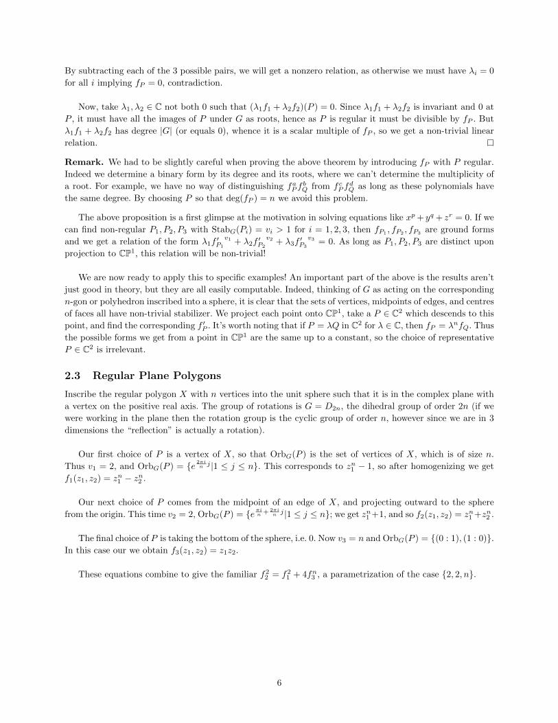
2.3 Regular Plane Polygons

Inscribe the regular polygon X with n vertices into the unit sphere such that it is in the complex plane with

a vertex on the positive real axis. The group of rotations is G = D2n, the dihedral group of order 2n (if we

were working in the plane then the rotation group is the cyclic group of order n, however since we are in 3

dimensions the “reflection” is actually a rotation).

Our first choice of P is a vertex of X, so that OrbG(P ) is the set of vertices of X, which is of size n.

Thus v1 = 2, and OrbG(P ) = e 2πin j |1 ≤ j ≤ n. This corresponds to zn1 − 1, so after homogenizing we get

f1(z1, z2) = zn1 − zn2 .

Our next choice of P comes from the midpoint of an edge of X, and projecting outward to the sphere

from the origin. This time v2 = 2, OrbG(P ) = eπin + 2πin j |1 ≤ j ≤ n; we get zn1 +1, and so f2(z1, z2) = zn1 +zn2 .

The final choice of P is taking the bottom of the sphere, i.e. 0. Now v3 = n and OrbG(P ) = (0 : 1), (1 : 0).In this case our we obtain f3(z1, z2) = z1z2.

These equations combine to give the familiar f22 = f2

1 + 4fn3 , a parametrization of the case 2, 2, n.

6

2.4 Octahedron

The group of rotations of the octahedron X has size 24 (it is in fact S4). Take the vertices of the octahedron

to be (using (x+ yi, z) to mean (x, y, z)):(0, 1

),

(1, 0

),

(i, 0

),

(− 1, 0

),

(− i, 0

),

(0,−1

).

We first take P to be a vertex, so v1 = 4. The vertices correspond to:

∞, 1, i,−1,−i, 0

which give us equation:

f1(z1, z2) = z1z2(z41 − z4

2).

Next, we take P to be the midpoint of an edge, so v2 = 2. The midpoints have coordinates:(1

2,

1

2

),

(i

2,

1

2

),

(− 1

2,

1

2

),

(− i

2,

1

2

),

(1 + i

2, 0

),

(−1 + i

2, 0

),(

−1− i2

, 0

),

(1− i

2, 0

),

(1

2,−1

2

),

(i

2,−1

2

),

(− 1

2,−1

2

),

(− i

2,−1

2

).

Rescaling to the sphere, we get:(√2

2,

√2

2

),

(√2i

2,

√2

2

),

(−√

2

2,

√2

2

),

(−√

2i

2,

√2

2

),

((1 + i)

√2

2, 0

),

((−1 + i)

√2

2, 0

),(

(−1− i)√

2

2, 0

),

((1− i)

√2

2, 0

),

(√2

2,−√

2

2

),

(√2i

2,−√

2

2

),

(−√

2

2,−√

2

2

),

(−√

2i

2,−√

2

2

).

Projecting downwards to the plane gives us:√2 + 1, (

√2 + 1)i,−(

√2 + 1),−(

√2 + 1)i,

(1 + i)√

2

2,

(−1 + i)√

2

2,

(−1− i)√

2

2,

(1− i)√

2

2,√

2− 1, (√

2− 1)i,−(√

2− 1),−(√

2− 1)i

,

from which we get:

f2(z1, z2) = z121 − 33z8

1z42 − 33z4

1z82 + z12

2 .

Finally, we take P to be the centre of a face, where v3 = 3. We get coordinates of the centres being:(1 + i

3,

1

3

),

(−1 + i

3,

1

3

),

(−1− i

3,

1

3

),

(1− i

3,

1

3

),(

1 + i

3,−1

3

),

(−1 + i

3,−1

3

),

(−1− i

3,−1

3

),

(1− i

3,−1

3

).

Projecting to the sphere yields:((1 + i)

√3

3,

√3

3

),

((−1 + i)

√3

3,

√3

3

),

((−1− i)

√3

3,

√3

3

),

((1− i)

√3

3,

√3

3

),(

(1 + i)√

3

3,−√

3

3

),

((−1 + i)

√3

3,−√

3

3

),

((−1− i)

√3

3,−√

3

3

),

((1− i)

√3

3,−√

3

3

).

Projecting downwards gives us:(1 + i)(

√3 + 1)

2,

(−1 + i)(√

3 + 1)

2,

(−1− i)(√

3 + 1)

2,

(1− i)(√

3 + 1)

2,

(1 + i)(√

3− 1)

2,

(−1 + i)(√

3− 1)

2,

(−1− i)(√

3− 1)

2,

(1− i)(√

3− 1)

2

,

7

from which we derive:

f3(z1, z2) = z81 + 14z4

1z42 + z8

2 .

Checking the coefficients of x24, x20y4 in the expansion of f41 , f

22 , f

33 yields the equation:

108f41 + f2

2 = f33 ,

which can be verified by multiplying out the terms.

2.5 Tetrahedron and Icosahedron

We could choose the octahedron to have friendly coordinates, which made the calculations not too bad, some-

thing which is less true in the tetrahedral and icosahedral cases. The process is the same as the octahedron:

for the points P , we choose a vertex, a midpoint of an edge, and the centre of a face. From this we get

exponent triples of 2, 3, 3 for the tetrahedron, and 2, 3, 5 for the icosahedron; these round out all possible sets

of exponents to make the generalized Fermat equation spherical. Instead of running through the calculations,

we will just present the final invariants that Beukers uses in his paper (the tetrahedral case is scaled so that

the coefficients are integers).

Tetrahedron:

f1 =z61 + 20z3

1z32 − 8z6

2

f2 =z1(z31 − 8z3

2)

f3 =z2(z31 + z3

2)

with the relation f21 − f3

2 − 64f33 = 0.

Icosahedron:

f1 =z301 − 522z25

1 z52 − 10005z20

1 z102 − 10005z10

1 z202 + 522z5

1z252 + z30

2

f2 =z201 + 228z15

1 z52 + 494z10

1 z102 − 228z5

1z152 + z20

2

f3 =z1z2(z101 − 11z5

1z52 − z10

2 )

with the relation f21 − f3

2 + 1728f53 = 0.

Remark. Our results can be applied to the cube and dodecahedron, however we do not get any new infor-

mation as these cases correspond to the results for the octahedron and icosahedron respectively.

Remark. In each case we found three orbits of G on the unit sphere where G does not act freely. If we found

another then we would get more relations of the form λ1f′P1

v1 + λ2f′P2

v2 + λ3f′P3

v3 = 0. However, by looking

at the stabilizer of each element of G, we see that the only possible orbits which G does not act transitively

on correspond to vertices, midpoints of edges, and centres of faces of our polyhedron.

2.6 Klein Forms

We derived polynomial relations geometrically, and there is a more algebraic interpretation of them which

comes from the study of covariants.

8

Definition 2.5. A generic form of order k is

f =

k∑i=0

(k

i

)aiz

k−i1 zi2.

Note the convention that the coefficients are not ai but

(k

i

)ai; this matches the notation historically used

in the study of covariants. As it turns out, it will also simplify the defining equation of the platonic solids

(see Proposition 4.5 and Appendix A).

From now on, g ∈ GL(2,C) acts on forms of order k by g · f = f g. This is no longer a group action

as (gh) · f = h · g · f , but this is of no concern to us. Let a = (a0, a1, . . . , ak), and let g · f correspond to

a′ = (a′0, a′1, . . . , a

′k).

Definition 2.6. A form C ∈ C[a0, a1, . . . , ak, z1, z2] is called a covariant if there exists a nonnegative integer

p such that

C(a′, z) = det(g)pC(a, gz)

for all g ∈ GL(2,C). The integer p is called the weight.

A common example of a covariant is the discriminant of a binary quadratic form; this has no zi terms

and is of weight 2 (hence invariant over SL(2,C)). We will be stating and using without proof various results

on covariants now and in Section 4. The theory of covariants is fully developed in Hilbert’s lecture notes on

algebraic invariants, [5], and most proofs can be found there.

For now, we only consider the following covariants:

H(f) =

(1

k(k − 1)

)2∣∣∣∣∣∣fxx fxy

fyx fyy

∣∣∣∣∣∣ = (a0a2 − a21)z2k−4

1 + · · ·

t(f) =1

k(k − 2)

∣∣∣∣∣∣ fx fy

Hx Hy

∣∣∣∣∣∣ = (a20a3 − 3a0a1a2 + 2a3

1)z3k−61 + · · ·

One can check that these are covariants of weights 2, 3 respectively. A motivation for their definition is they

appear naturally when applying the transvectant process, which creates covariants from a pair of forms.

When Klein embedded the regular solids into the unit sphere and projected their vertices onto CP1, he

obtained f(z1, z2), and relations involving f , H(f), and t(f).

r Solid Form βr

3 Tetrahedron f3 = z42 − 2

√3z2

1z22 − z4

1 3√

3

4 Octahedron f4 = z1z2(z41 − z4

2) 432

5 Icosahedron f5 = z1z2(z102 − 11z5

1z52 − z10

1 ) 1738

The relations he derived are: (1

2t(fr)

)2

+ H(fr)3 +

1

βrfrr

= 0

for r = 3, 4, 5.

9

Definition 2.7. For r = 3, 4, 5 and d ∈ C∗ define:

C (r) =fr g|g ∈ GL(2,C)

C (r, d) =

f ∈ |

(1

2t(f)

)2

+ H(f)3 + dfr = 0

For f ∈ C (r, d) define

χ(f) : C2 → C3

(z1, z2)→ (1

2t(f),H(f), f).

Note that fr ∈ C (r, 1βr

).

Lemma 2.8. Suppose f ∈ C (r, d). Then:

• If g ∈ GL(2,C), then f g ∈ C (r, det(g)6d).

• If µ ∈ C∗, then µf ∈ C (r, µ6−rd).

Proof. Clear, using that H and t are covariants of weights 2, 3.

Definition 2.9. Call C (3) ∪ C (4) ∪ C (5) the Klein forms.

The algebraic approach given here will be the main tool in Section 4, where we compute explicit solu-

tions. For the intervening sections we will however mostly ignore this, and focus on the geometric approach

originally described.

3 Parametrized Solutions

3.1 Some Preliminaries

We will start by recapping the results of the previous section in a table. Note that we have permuted and

rescaled some the polynomials fi of the previous section to make nicer relations.

Figure (p, q, r) f1 f2 f3 Relation

n−gon (2, 2, n) zn1 − zn2 zn1 + zn2 z1z2 f21 − f2

2 + 4fn3 = 0

Tetrahedron (2, 3, 3) z61 + 20z3

1z32 − 8z6

2 z1(z31 − 8z3

2) z2(z31 + z3

2) f21 − f3

2 − 64f33 = 0

Octahedron (2, 3, 4) z121 − 33z8

1z42 − 33z4

1z82 + z12

2 z81 + 14z4

1z42 + z8

2 z1z2(z41 − z4

2) f21 − f3

2 + 108f43 = 0

Icosahedron (2, 3, 5) * * * f21 − f3

2 + 1728f53 = 0

For the icosahedron we have:

f1 =z301 − 522z25

1 z52 − 10005z20

1 z102 − 10005z10

1 z202 + 522z5

1z252 + z30

2

f2 =z201 + 228z15

1 z52 + 494z10

1 z102 − 228z5

1z152 + z20

2

f3 =z1z2(z101 − 11z5

1z52 − z10

2 )

Let S be a finite set of primes and A,B,C be nonzero integers. Let (p, q, r) be one of the above triples,

and consider the equation

Axp +Byq + Czr = 0 with (x, y, z) ∈ Z3, (3.1)

10

with the restriction that

xyz 6= 0 and p - gcd(x, y, z) for all p /∈ S. (3.2)

Let G be the group of rotations corresponding to the triple (p, q, r). By rescaling f1, f2, f3, we have poly-

nomials h1(s, t), h2(s, t), h3(s, t) ∈ C[s, t] such that Ahp1 + Bhq2 + Chr3 = 0. Let V be the zero set of

F (x, y, z) = Axp +Byq + Czr in C3.

The main result of this essay is the following theorem, which is proved in the next section.

Theorem 3.1. There exist a finite set of polynomial triples Fi = (fi, gi, hi) ∈ Q[z1, z2]3, 1 ≤ i ≤ r such that

if (x, y, z) is a solution to equations 3.1 and 3.2, then there exist integers z1, z2 and i with 1 ≤ i ≤ r such

that (x, y, z) = Fi(z1, z2). In more informal terms, there is a finite list of two variable polynomials over Qsuch that all solutions to to equations 3.1 and 3.2 can be obtained by specializing the inputs to be integers.

The rest of this subsection is spent on setting up the proof of the above theorem. Define:

φ : C2 → V

(x, y)→ (h1(x, y), h2(x, y), h3(x, y))

Proposition 3.2. The map φ : C2 → V is surjective.

Proof. Let X,Y, Z ∈ V , and consider h2(x, y) = Y, h3(x, y) = Z. Let di = deg(hi), and then this is equivalent

to h2(x/y, 1) = Yyd2

and h3(x/y, 1) = Zyd3

, so Zd2h2(x/y, 1)d3 = Y d3h3(x/y, 1)d2 . This is a polynomial in the

variable x/y, so it has a root r say, and then we can choose an appropriate y so that h2(r, 1) = Yyd2

and

h3(r, 1) = Zyd3

. Taking x = yr, we have a solution to h2(x, y) = Y, h3(x, y) = Z. Considering the defining

equation for V , this gives X2 = h1(x, y)2, so h1(x, y) = ±X. If it is X then we are done, so assume otherwise.

We will be done if we find a matrix m such that h1 m = −h1 and hi m = hi for i = 2, 3. Considering

our expressions for fi above, we see that we can take m to be (ζ8 is a primitive 8th root of unity):0 1

1 0,

,

i 0

0 i,

,

0 ζ8

ζ−18 0,

,

i 0

0 i,

for the n−gon, tetrahedral, octahedral, and icosahedral cases respectively.

Remark. For clarity we did the above over C, but it clearly remains true when working over an algebraically

closed field of characteristic 0. We will be using it for Q.

We will run into a slight problem when φ is not defined over Q, as there can be different conjugates of

φ, namely φσ = σφσ−1 for σ ∈ Gal(Q/Q). As it turns out, there exists a linear polynomial homeomorphism

p (i.e. p ∈ GL(2,Q)) such that φσ = φ p. The proof is a result of the more general Theorem 1.3 of [1].

Alternatively, one can check this explicitly from our equations for f1, f2, f3. For example, in the n-gon case,

we have

h1 = af1, h2 = bf2, h3 = cf3

a =

√1

A, b =

√1

−B, c =

n

√4

C

As A,B,C are integers, φσ = φ · (±1,±1, ζ) with multiplication taken pointwise, some choice of signs ±(depending on if A,−B are rational squares) and ζ being an nth root of unity. Letting η be a nth root of −1,

then we can then choose p to be

11

Case p Case p

(1, 1, ζ)(

1 00 ζ

)(1,−1, ζ)

( 0 ηζ

η−1 0

)(−1, 1, ζ)

(0 ζ1 0

)(−1,−1, ζ)

( ηζ 0

0 η−1

)The other cases can be checked similarly. Define:

G = g ∈ GL(2,Q)|∃σ ∈ Gal(Q/Q) : φσ = φ g.

Note that G contains G but is not necessarily a group. The use of G is found in the following proposition.

Lemma 3.3. Suppose φσ(v) = φ(u) for some u,v ∈ C2, where u is regular. Then there exists a unique

g ∈ G such that g(v) = u.

Proof. Let p ∈ GL(2,Q) be such that φσ = φ p. Thus we have φ(p(v)) = φ(u). Let w = p(v); then

hi(w) = hi(u) for i = 1, 2, 3. As any three ground forms are linearly dependent, and he11 ,he22 are two linearly

independent ground forms which take the same value at u,w, we see that all ground forms agree at u,w.

In particular, 0 = fw(w) = fw(u), so u is a root of fw, and thus u = λg1w for some g1 ∈ G, λ ∈ C∗. As

hi(w) = hi(u) for each i, we see λ = ±1, and if it is −1 then it can be absorbed into g1. Thus u = g1 p(v),

so let g = g1 p. We have φσ = φ p = φ g1 p = φ g, so g ∈ G, and thus we have existence. Note that we

did not need u to be regular for existence.

To show uniqueness, assume we have g = g1 p and g′ = g2 p′ which work. Thus φσ = φ p = φ p′, so

as above we have a g3 ∈ G such that p = g3 p′. Thus g′ = (g2g3) p. However, u being regular implies that

given p, the choice of g1 we made was unique, thus g1 = g2g3 and g = g′.

Definition 3.4. A matrix m ∈ GL(2,Q) such that φ m is defined over Q is called a Q−matrix.

Note that Proposition 3.2 implies that all parametrized solutions of degree |G| arise from Q−matrices.

Definition 3.5. If m is a Q−matrix, then for any g ∈ G and r ∈ GL(2,Q) we have g m r is also a

Q−matrix. Call these matrices equivalent; this is an equivalence relation on Q−matrices.

The path ahead is now fairly clear. Twisting φ by two equivalent Q−matrices will produce two polynomials

with rational coefficients, which output the same set of values when the inputs are taken to be rational. Thus

the goal is to show that there are finitely many equivalence classes of Q−matrices from which all solutions

with the restriction in equation 3.2 can be derived.

3.2 Proof of the Main Result

Note that enlarging the set S by a adding in a finite number of primes does not change the generality of The-

orem 3.1. We will enlarge S so that the following conditions are met (OS is the ring of S−integral algebraic

integers):

1) S contains the primes ramifying in the fields of definition of G and φ (and thus G);

2) G ⊂ GL(2,OS);

3) h1, h2, h3 ∈ OS [z1, z2]

4) If p is a prime not above a prime in S, then the natural reduction map G → GL(2) (mod p) is injective.

We continue with a lemma and a proposition, before moving on to the actual proof of Theorem 3.1.

Lemma 3.6. Let m be a Q−matrix. Then for every σ ∈ Gal(Q/Q), let gσ = mσ(m)−1. Then we have

gσ ∈ G.

12

Proof. First, take h ∈ G such that φσ = φ h. Thus we get:

φ m = σ(φ m) = φσ(σ(m)) = φ h σ(m),

so thus there must exist g ∈ G such that m = gh σ(m), so gσ = gh ∈ G.

Proposition 3.7. Let t = (x, y, z) be a solution of equations 3.1 and 3.2. Then there exists a Q−matrix m

and s ∈ Q2 such that t = (φ m)(s). Furthermore, the equivalence class of m is uniquely determined by t,

and the field generated by the elements of m is unramified outside of S.

Proof. Take u ∈ Q2such that t = φ(u). Since xyz 6= 0, we see that u is a regular vector. Let σ ∈ Gal(Q/Q),

so φσ(σ(u)) = σ(t) = t = φ(u); as u is regular we have by Lemma 3.3 there exists a unique gσ ∈ G such that

gσσ(u) = u.

For σ ∈ Gal(Q/Q), note that since

φσ(g−1σ u) = φσ σ(u) = t = φ(u) = φ gσ(g−1

σ u)

we get that this must be true in general, i.e. φσ = φ gσ (it is true for a unique g ∈ G, and true with g = gσfor g−1

σ u, a regular vector). Therefore for φ, σ ∈ Gal(Q/Q)

φ (gσσ(gτ )(r)) = φσ(σ(gτ )(r)) = σ(φ(gτ (σ−1(r)))) = σ(φτ (σ−1(r))) = φστ (r)

whence we have the cocycle property, gστ = gσσ(gτ ). Hilbert’s 90 forGL(n) states thatH1(Gal(Q/Q), GL(n,Q)) =

0, so we conclude that there exists a m ∈ GL(2,Q) such that gσ = mσ(m)−1 for all σ ∈ Gal(Q/Q).

We have:

σ(φ m) = φσ σ(m) = φσ g−1σ m = φ m,

for all σ ∈ Gal(Q/Q), whence m is a Q−matrix. Also, φ m(m−1(u)) = t, and for σ ∈ Gal(Q/Q) we have

σ(m−1(u)) = m−1gσ(σ(u)) = m−1(u).

So s = m−1(u) ∈ Q2 and (φ m)(s) = t.

Next, we need to show the uniqueness of the equivalence class of m. Assume that we also have a Q−matrix

m′ and s′ ∈ Q so that

t = (φ m′)(s′) = (φ m)(s) = φ(u).

As u is regular, there exists a unique g ∈ G with m(s) = gm′(s′). Since we consider the equivalence class of m,

we can assume WLOG that g = id and u = m(s) = m′(s′). From Lemma 3.6, we have for all σ ∈ Gal(Q/Q)

a gσ, g′σ ∈ G such that

gσ =mσ(m)−1

g′σ =m′σ(m′)−1.

Therefore we get

σ(u) =σ(m(s)) = g−1σ (m(s)) = g−1

σ u (3.3)

σ(u) =σ(m′(s′)) = (g′σ)−1(m′(s′)) = (g′σ)−1u (3.4)

whence gσ = g′σ for all σ ∈ Gal(Q/Q). Rearranging mσ(m)−1 = gσ = g′σ = m′σ(m′)−1 implies m−1m′ =

σ(m−1m′), whence m−1m′ ∈ GL(2,Q), i.e. m and m′ are equivalent.

13

For the last part, let K be the normal closure of the field generated by the elements of m, let p /∈ S be

prime, and let p be a prime in OK above p. Taking Ip to be the inertia group of p, to show p is unramified we

need to show that this group is trivial. Assumptions 2, 3 imply that the map φ descends to a map φ (mod p)

which is a quotient map for G (mod p). As t = φ(u) does not descend to 0, u (mod p) is a regular vector for

G (mod p). For σ ∈ Ip, σ(u) ≡ u (mod p), and so using equation 3.3 and u being regular, we get gσ ≡ id

(mod p). Since G injects into GL(2) (mod p), we get that gσ = id, so σ(m) = m for all σ ∈ Ip. By definition

of K we get σ = id, so Ip is trivial, and p is unramified in K.

Remark. One can in fact avoid using Hilbert’s 90 and explicitly construct m: there exist invariants I1, I2such that the matrix of partial derivatives

J =

∂I1∂z1

∂I1∂z2

∂I2∂z1

∂I2∂z2

,

evaluated at u has nonzero determinant. One can check that m = J(u)−1 satisfies the desired equation

gσ = mσ(m)−1 for all σ ∈ Gal(Q/Q).

Proposition 3.8. There is a finite set M of Q−matrices such that for every solution t of equations 3.1 and

3.2, there exists m ∈M and s ∈ Q2 such that t = (φ m)(s).

Proof. Using Proposition 3.7, we can choose M to be a set of non-equivalent Q−matrices satisfying the

proposition; it remains to show that M is finite.

Let K be a number field over which G is defined. Pick m ∈M , and let L be the field over K generated by

the elements of m. If d is the degree of the field of definition of φ, then we know the size of G is at most d|G|.But we also know that for σ ∈ Gal(Q/Q), σ(m) = g−1

σ m whence L is normal over K and [L : K] ≤ d|G|.Proposition 3.7 also tells us that L is unramified outside of the finite set S, so by Hermite’s theorem there

are finitely many choices for L.

The final step is given an L, there are finitely many m ∈M which give rise to L. Indeed, the map

Gal(Q/Q)→Gσ →gσ

factors over Gal(L/Q), and there are finitely many maps Gal(L/Q)→ G. As checked in Proposition 3.7, two

Q−matrices giving rise to the same map are equivalent, completing the proposition.

The above proposition is almost the result we claimed: we wish to take the inputs of parametrized solutions

to be integers, and currently we have them as rational numbers. We will now fix this to prove Theorem 3.1.

Lemma 3.9. Let g1, g2 ∈ Q[z1, z2] be coprime homogeneous polynomials of positive degree. Let Λ be the

Z−module spanned by all s ∈ Q2 such that gi(s) ∈ Z for i = 1, 2. Then Λ is a lattice of rank 2.

Proof. By clearing the denominators of the gi, we can assume WLOG that gi ∈ Z[z1, z2] for i = 1, 2. It is

sufficient to show that there exists an integer N such that NΛ ⊂ Z2. Assume this statement is false; then there

are arbitrarily large integers N such that there exist a, b ∈ Z with at least one of a, b coprime to N such that

g1( aN ,bN ), g2( aN ,

bN ) ∈ Z. Multiplying through by N , we get Nk1 | g1(a, b) and Nk2 | g2(a, b) with ki being the

degree of gi. As g1, g2 are coprime, we can run Euclid’s algorithm on g1(1, z2z1 ), g2(1, z2z1 ) and g1( z1z2 , 1), g2( z1z2 , 1)

and multiply thorough by a certain power of z1, z2 to get polynomials A1, A2, B1, B2 ∈ Z[z1, z2] such that

A1g1 +A2g2 =Aze11

B1g1 +B2g2 =Bze22

14

for some integer constants A,B, and positive integers e1, e2. Plugging in (z1, z2) = (a, b), we see that as

ki ≥ 1, we have N | Aae1 , Bbe2 . But N is coprime to one of a, b whence N | A or N | B. In any case,

|N | ≤ |AB| whence such arbitrarily large N cannot exist.

Proof of Theorem 3.1. Let m be a Q−matrix. Let Λ(m) be the set of s ∈ Q2 such that φ m(s) ∈ Z2. By

the above lemma, this is a Z−lattice of rank two, so let it be generated by s1, s2. Therefore replacing φm(z)

by g(z1, z2) = φ m(s1z1 + s2z2) means that all integral values that φ m takes are in g(Z2). Repeat this for

the finite set of non-equivalent Q−matrices to deduce the theorem.

4 Constructing Explicit Solutions

4.1 Restricting to Klein Forms

We will now be studying Klein forms, which only seem to parametrize solutions to Ax2 + By3 + Czr = 0

when A = B = 1. However, multiply by A3B2 to get:

(A2Bx)2 + (ABy)3 +A3B2Czr = 0.

Thus by restricting to the case A = B = 1 we lose no generality; when we give our final algorithm we will

comment on the changes which must be made.

4.2 Classification of Klein Forms

To determine the parametrizations of the generalized Fermat equation, it suffices to determine the Klein

Forms. It turns out there is a quite simple algebraic characterization of them, which will form the basis of an

algorithm to calculate integer parametrizations explicitly. We inherit the notation and conventions of Section

2.6; in particular recall that a general form of order k is written as

f =

k∑i=0

(k

i

)aiz

k−i1 zi2.

For any k, define the 4th and 6th covariants of a form f of order k by:

τ4(f) =1

2

((k − 4)!

k!

)2

Ω4f(x, y)f(x′, y′)

∣∣∣∣x,x′=z1y,y′=z2

τ6(f) =1

2

((k − 6)!

k!

)2

Ω6f(x, y)f(x′, y′)

∣∣∣∣x,x′=z1y,y′=z2

with

Ω =

(δ2

δxδy′− δ2

δyδx′

).

The first term is given by

τ4(f) =(a0a4 − 4a1a3 + 3a22)z2k−8

1 + · · · ,τ6(f) =(a0a6 − 6a1a5 + 15a2a4 − 10a2

3)z2k−121 ;

these are (up to a constant) the 4th and 6th transvectants of f with itself, and have weight 4, 6 respectively.

The next three results are proved (or a reference is given) in Edwards’s paper [6]. The main ideas essentially

come from the algebraic relations that being a covariant implies; see Hilbert’s lecture notes [5] for more detail.

15

For forms of order 4, define the catalecticant invariant j by

j(f) =

∣∣∣∣∣∣∣∣a0 a1 a2

a1 a2 a3

a2 a3 a4

∣∣∣∣∣∣∣∣=a0a2a4 + 2a1a2a3 − a3

2 − a0a3 − a21a4

which is covariant of weight 6.

Theorem 4.1 (Gordan 1887). Let f be a form of order k. Then τ4(f) = 0 if and only if f is GL(2,C)

equivalent to zk1 , zk−11 z2, or one of the Klein forms f3, f4, or f5.

Lemma 4.2. Let C be a covariant of weight p, homogeneous of degree n in the ai. If p > n, then C(zk1 ) =

C(zk−11 z2) = 0.

Theorem 4.3 (Classification of Klein Forms). Fix d ∈ C∗. Then:

C (3, d) =f ∈ C[z1, z2]4|τ4(f) = 0, j(f) = 4d,C (4, d) =f ∈ C[z1, z2]6|τ4(f) = 0, τ6(f) = 72d,

C (5, d) =

f ∈ C[z1, z2]12

∣∣∣∣τ4(f) = 0, τ6(f) =360

7df

,

The proof of the classification is a consequence of the previous theorem and lemma, along with a calcu-

lation done for the forms fr that Klein found (Section 2.6). The classification generates a list of polynomials

equations in the ai, which are necessary and sufficient for f to be a Klein form. This is the first key ingredient

in generating explicit solutions.

The two defining equations for the tetrahedron are:

0 =a0a4 − 4a1a3 + 3a22 (4.1)

4d =a0a2a4 + 2a1a2a3 − a32 − a0a

23 − a2

1a4. (4.2)

We list the equations for the Octahedron and Icosahedron in Appendix A; these calculations were done by

Edwards in Appendix A of [7].

4.3 Lifting Integer Solutions

This subsection is the parallel to finding a Q−matrix associated to an integral solution. The upshot of the

method presented here is we get a lot more information on the coefficients of the form f .

To define what it means for a form to be integral, we use a slightly funny definition.

Definition 4.4. For r ∈ 3, 4, 5 define:

U3 =a0, . . . , a4,U4 = a0, . . . , a6U5 =a0, . . . , a5, 7a6, a7, . . . , a12

For f a form of order k (k = 4, 6, 12 respective to r = 3, 4, 5), denote Ur(f) to be the specialization of Ur to

the coefficients of f . For a ring R ⊂ C, define

C (r, d)(R) = f ∈ C (r, d)|Ur(f) ⊂ R;

we call such forms R−integral.

16

Remark. Since GL(2,Z) is generated by(

0 1−1 0

),(

1 10 1

),(

1 00 −1

), it is easy to check that C (r, d)(Z) is closed

under the action of GL(2,Z).

Proposition 4.5. Let d be a nonzero integer and r ∈ 3, 4, 5. If (X,Y, Z) satisfy X2 + Y 3 + dZr = 0

where X,Y, Z are coprime integers, then there exists a form f ∈ C (r, d)(Z) and s = (s1, s2) ∈ Z2 such that

χ(f)(s1, s2) = (X,Y, Z) (χ is defined in Definition 2.7).

Proof. Pick any f ∈ C (r, d). Proposition 3.2 implies that there exist (s1, s2) ∈ C2 such that χ(f)(s1, s2) =

(X,Y, Z) (all parametrizations are GL(2,C) twists of each other). By applying a transformation in SL(2,C)

we can assume that (s1, s2) = (1, 0), and so we have the equations:

2X =t(1, 0) = a20a3 − 3a0a1a2 + 2a3

1

Y =H(1, 0) = a0a2 − a21

Z =f(1, 0) = a0.

(4.3)

Note for λ ∈ C, replacing f(z1, z2) by f(z1 + λz2, z2) corresponds to(

1 λ0 1

), so our form remains in C (r, d)

and the above equations for X,Y, Z remain unchanged. We will now show how to choose λ so that the re-

sulting form is in C (r, d)(Z), which will complete the proof. We will use the above three equations to play

with a0, a1, a2, a3, and use the defining equations of the Klein forms to deduce the result for the rest of the

coefficients.

Case 1: Z = 0

We have a0 = 0, and since Klein forms are separable (just check f3, f4, f5) we must have a1 6= 0. Therefore

we can choose λ making a2 = 0. Plugging this into equations 4.3 and using the coprimality of X,Y, Z = 0,

we see that a1 = ±1 and (X,Y, Z) = (±1,−1, 0).

For the tetrahedron case, the defining equations 4.1 imply that

(a0, a1, . . . , a4) = (0,±1, 0, 0,−4d),

so indeed, U3(f) ⊂ Z, as required. The octahedral and icosahedral cases can be completed in similar fashion.

Case 2: Z 6= 0

This case requires a bit more work; as a0 = Z 6= 0, varying λ implies that we can take a1 to be any value we

like. Note that Y, Z must be coprime, so we can take a1 to be an integer satisfying:

a1 ≡ −X

Y(mod Zr)

This equivalence can be reverse engineered from the resulting expressions for a2, a3 (from equations 4.3):

a0a2 =Y + a21 ≡ Y +

(X

Y

)2

=−dZr

Y 2≡ 0 (mod Zr)

a20a3 =2X + 3a0a1a2 − 2a3

1 ≡ 2X − 2

(− X

Y

)3

≡ 2X−dZr

Y 3≡ 0 (mod Zr),

(noting that the first equation implies Zr−1 | a0 whence Zr | 3a0a1a2.

In particular, this imples that a0, a1, a2, a3 ∈ Z and for any prime p dividing Z they satisfy:

p1||a0, p0||a1, pr−1|a2, pr−2|a3.

For the tetrahedron, our equation for a4 is:

a0a4 = 4a1a3 − 3a22

from which it follows that a4 ∈ Z and f ∈ C (3, d)(Z). The octahedral and icosahedral cases can be completed

in similar fashion.

17

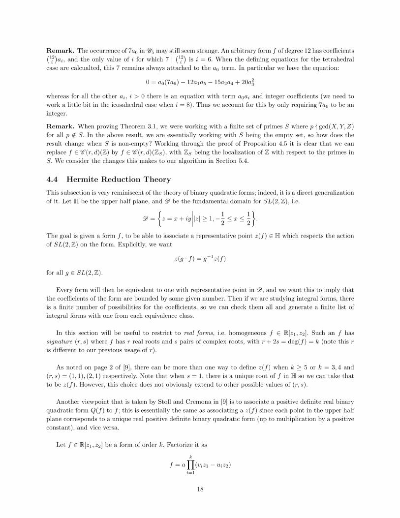
Remark. The occurrence of 7a6 in U5 may still seem strange. An arbitrary form f of degree 12 has coefficients(12i

)ai, and the only value of i for which 7 |

(12i

)is i = 6. When the defining equations for the tetrahedral

case are calcualted, this 7 remains always attached to the a6 term. In particular we have the equation:

0 = a0(7a6)− 12a1a5 − 15a2a4 + 20a23

whereas for all the other ai, i > 0 there is an equation with term a0ai and integer coefficients (we need to

work a little bit in the icosahedral case when i = 8). Thus we account for this by only requiring 7a6 to be an

integer.

Remark. When proving Theorem 3.1, we were working with a finite set of primes S where p - gcd(X,Y, Z)

for all p /∈ S. In the above result, we are essentially working with S being the empty set, so how does the

result change when S is non-empty? Working through the proof of Proposition 4.5 it is clear that we can

replace f ∈ C (r, d)(Z) by f ∈ C (r, d)(ZS), with ZS being the localization of Z with respect to the primes in

S. We consider the changes this makes to our algorithm in Section 5.4.

4.4 Hermite Reduction Theory

This subsection is very reminiscent of the theory of binary quadratic forms; indeed, it is a direct generalization

of it. Let H be the upper half plane, and D be the fundamental domain for SL(2,Z), i.e.

D =

z = x+ iy

∣∣∣∣|z| ≥ 1,−1

2≤ x ≤ 1

2

.

The goal is given a form f , to be able to associate a representative point z(f) ∈ H which respects the action

of SL(2,Z) on the form. Explicitly, we want

z(g · f) = g−1z(f)

for all g ∈ SL(2,Z).

Every form will then be equivalent to one with representative point in D , and we want this to imply that

the coefficients of the form are bounded by some given number. Then if we are studying integral forms, there

is a finite number of possibilities for the coefficients, so we can check them all and generate a finite list of

integral forms with one from each equivalence class.

In this section will be useful to restrict to real forms, i.e. homogeneous f ∈ R[z1, z2]. Such an f has

signature (r, s) where f has r real roots and s pairs of complex roots, with r + 2s = deg(f) = k (note this r

is different to our previous usage of r).

As noted on page 2 of [9], there can be more than one way to define z(f) when k ≥ 5 or k = 3, 4 and

(r, s) = (1, 1), (2, 1) respectively. Note that when s = 1, there is a unique root of f in H so we can take that

to be z(f). However, this choice does not obviously extend to other possible values of (r, s).

Another viewpoint that is taken by Stoll and Cremona in [9] is to associate a positive definite real binary

quadratic form Q(f) to f ; this is essentially the same as associating a z(f) since each point in the upper half

plane corresponds to a unique real positive definite binary quadratic form (up to multiplication by a positive

constant), and vice versa.

Let f ∈ R[z1, z2] be a form of order k. Factorize it as

f = a

k∏i=1

(viz1 − uiz2)

18

with a ∈ C∗. For ti ∈ R∗, 1 ≤ i ≤ k, define φ(t) by

φ(t) =

k∑i=1

t2i (viz1 − uiz2)(viz1 − uiz2) =

k∑i=1

t2i |viz1 − uiz2|2.

Note that φ is then a positive definite real quadratic form! Let δ be its determinant, i.e. if φ = Az21 +2Bz1z2 +

Cz22 then δ = AC −B2 > 0.

As it turns out, the key is to look at an expression introduced by Hermite in [4]

Φ(t) =|a|2δk/2

(∏ti)2

Definition 4.6. For a form f ∈ R[z1, z2] and any z ∈ C, define the Hermite Covariant as

Θ(f, z) =

min Φ(t) over all t such that φ(z, 1) = 0,

∞ if φ(z, 1) = 0 for all t.

We now check that the definition of Θ is independent of the choice of a, ui, vi. Indeed, if

f = a′k∏i=1

(v′iz1 − u′iz2)

corresponds to φ′,Φ′, then we have some c, c1, c2, . . . , ck ∈ C such that

a′ = ca, u′i = ciui, v′i = civi, cc1c2 · · · ck = 1

Let t′ = ( t1|c1| , . . . ,

tk|ck| ), and we have

φ′(t′) =

k∑i=0

(ti|ci|

)2

|v′iz1 − u′iz2|2 =

k∑i=0

t2i |viz1 − uiz2|2 = φ(t).

Therefore φ(z, 1) = φ′(z, 1), and if φ(z, 1) = 0 then we have

Φ′(t′) =|a′|2δk/2

(∏t′i)

2=|a|2|c|2δk/2

(∏ti/|ci|)2

= Φ(t),

since |cc1c2 · · · ck|2 = 1. For Θ, we take the minimum of Φ(t) over all t, whence the different expressions for

f produce the same Θ, so it is well defined.

Definition 4.7. For a form f ∈ R[z1, z2] define the Hermite determinant as

Θ(f) = minz∈H

Θ(f, z).

Definition 4.8. For any form f ∈ R[z1, z2], a representative point is any z ∈ H such that Θ(f, z) = Θ(f).

Definition 4.9. A form f ∈ R[z1, z2] is called Hermite reduced if it has a representative point in D .

For an example, consider f to be a positive definite real binary quadratic form, say with leading coefficient

1. Then as the roots are complex conjugates, we get φ = (t21 + t22)f , and so Θ(f, z) is undefined for all z apart

from the two roots of f(z, 1), where it is ∞. So the Hermite determinant is ∞, and the representative point

agrees with the notion of a representative point for a binary quadratic form. Thus f is Hermite reduced if

19

and only if f is reduced as a positive definite binary quadratic form.

Lemma 4.2 of [9] implies that if our form f has order at least 3 and has distinct roots, then the represen-

tative point in unique. As Klein forms have distinct roots and order at least 3, we will assume this from now

on and denote the unique representative point by z(f).

We now have a series of results which allow us to bound coefficients of a Hermite reduced form. It essen-

tially follows the sequence of results in Section 4 of [6].

Proposition 4.10. Let f ∈ R[z1, z2] be a form of order k. Then for g ∈ GL(2,R) we have

Θ(f g, z) = |det(g)|kΘ(f, gz).

Therefore Θ(f g) = |det(g)|kΘ(f).

Proof. This is clear from carefully plugging f g into the definition of Θ.

Corollary 4.11. Let f ∈ R[z1, z2] be a form of order k, and g ∈ GL(2R). Then

z(g · f) = g−1z(f)

Proof. This immediately follows from Proposition 4.10.

Thus we have justified that our choice of representative point is a reasonable way to define a reduction

theory.

4.5 Bounds on Hermite Reduced Forms

We start off with a few results which produce bounds on the coefficients of f in terms of Θ (see Theorem

4.2.5 and Appendix A of [6]).

Denote 1, . . . , n by [n], and if S ⊂ [n] let S′ = [n]\S. If b ∈ Ck, let bS =∏i∈S bi.

Lemma 4.12. Let bi, ci ∈ C with∑ki=1 |bi|2 =

∑ki=1 |ci|2 = 1. Then∣∣∣∣ ∑

S⊂[k],|S|=r

bS′cS

∣∣∣∣ ≤ (kr)(

1

k

)k/2Proof. By the triangle inequality and Cauchy-Schwartz, we have∣∣∣∣ ∑

S⊂[k],|S|=r

bS′cS

∣∣∣∣2 ≤ ( ∑|S|=r

|bS′cS |)2

≤( ∑|S|=r

|bS′ |2)( ∑

|S|=r

|cS |2).

Generalized AM-GM ([2], page 15, exercise 22) gives( ∑|S|=r

|bS′ |2)≤(

k

k − r

)(∑ki=1 |bi|2

k

)k−r,

( ∑|S|=r

|cS |2)≤(k

r

)(∑ki=1 |ci|2

k

)r.

Combining inequalities and using∑ki=1 |bi|2 =

∑ki=1 |ci|2 = 1,

(kk−r)

=(kr

)gives the result.

Theorem 4.13. Let f =∑ki=0

(ki

)aiz

k−i1 zi2 be a real form of order k, and let z = x + iy ∈ H. Then for all

0 ≤ r ≤ k,

|ar|2 ≤|z|2r

(ky)kΘ(f, z)

20

Proof. For simplicity, denote Θ = Θ(f, z). Write f =∏ki=1(viz1 − uiz2); by the definition of Θ, there exists

ti > 0 so that

Θ =δk/2

(∏ti)2

where δ is the determinant of the positive definite quadratic form φ(z1, z2) = Pz21 − 2Qz1z2 + Rz2

2 , where

φ(z, 1) = 0 and

P =∑

t2i |vi|2, 2Q =∑

t2i (uivi + uivi), R =∑

t2i |ui|2.

Using z = x+ iy, we have

x =Q

P, |z|2 =

R

P

and thus

δ = PR−Q2 = P 2|x+ iy|2 − P 2x2 = P 2y2

Rearranging our expression for Θ gives 1 =√

Θδk/4

∏ti, so

f =

√Θ

δk/4(∏

ti)f =

√Θ

(Py)k/2

k∏i=1

(tiviz1 − tiuiz2).

Let bi = viti√P

and ci = −uiti√R

; then∑|bi|2 =

∑|ci|2 = 1. We have(

k

r

)ar =

√Θ

yk/2

∑S⊂[k],|S|=r

( ∏i∈S′

tivi√P

)(∏i∈S

−tiui√P

)

=

√Θ

yk/2

(√R√P

)r ∑S⊂[k],|S|=r

( ∏i∈S′

bi)(∏

i∈Sci)

=

√Θ|z|r

yk/2

∑S⊂[k],|S|=r

bS′cS

Apply Lemma 4.12 to deduce the result.

Theorem 4.14. Let

f(z1, z2) =

k∑i=0

(k

i

)aiz

k−i1 zi2

be a real form of order k. If f is Hermite reduced, then

|aiaj | ≤(

4

3k2

) k2

Θ(f)

whenever i+ j ≤ k.

Proof. Let z = x+iy be the representative point of f . As it is in the fundamental domain, y ≥√

3

2max1, |z|.

Use this in Theorem 4.13 to cancel the |z| and y terms, from which we deduce the result.

We now need to be able to calculate Θ(f).

Proposition 4.15. Let f = a∏i(viz1−uiz2) be a real form of order k ≥ 3 with distinct roots. If z = x+iy ∈ H

is the representative point, then

Θ(f) =

(k

2y

)k|a|2

k∏j=1

(|vjx− uj |2 + |vjy|2).

21

Proof. This follows from Proposition 5.1 of [9] when all the roots of f are finite (the definition of Θ used in

[9] differs from ours by the constant factor ( 2k )k). When f has an infinite root, an application of Propositon

4.10 does the trick.

Thus given a form and its representative point, we have a way to compute its Hermite determinant. We

will need some more information on the representative point; how to calculate it for forms of order 4 and

what it is for fr will suffice.

Looking at the definition of φ, one can see that weights t2i which give the Hermite determinant must be

equal for the pairs of complex conjugate roots. Thus we will assign weights t21, . . . , t2r to the real roots and

u21, u

21, . . . , u

2s, u

2s to the complex roots.

Proposition 4.16. Let f be a real form of order 4 with all roots finite. Then the weights ti which cause the

Hermite determinant to be obtained are given in the following table:

Signature Roots Weights

(4, 0) α1, α2, α3, α4 t2i =1

| ∂f∂z1 (αi, 1)|(2, 1) α1, α2 t21 = |β − β||α2 − β|2, t22 = |β − β||α1 − β|2

β, β u21 = |α1 − α2||α1 − β||α2 − β|

(0, 2) β1, β1 u21 = |β2 − β2|

β2, β2 u22 = |β1 − β1|

Proof. See Proposition 4.2.4 of [6].

Lemma 4.17. The representative point of f3, f4, f5 is i.

Proof. See Proposition 4.24, Lemma 4.26 in [6]. The key point for f4, f5 is f(z2,−z1) = ±f(z1, z2).

Proposition 4.18. Let f ∈ C (r, d)(R). Then f has a real root.

Proof. We can assume that f has no infinite root by applying a suitable transformation. Recalling Section 2,

we can inscribe the platonic solid corresponding to d into the unit sphere, so that the roots of f correspond

to the projection of the vertices onto the plane. Note that for each the tetrahedron, octahedron, and icosa-

hedron, if a circle goes through an even number of points, then it goes through at most 4. Furthermore, if it

goes through 4, then the two regions of the sphere formed also contain vertices of the solid. Under projection,

circles go to circles and these properties are transferred to the plane.

If f has no real root, then all of its roots come in complex conjugate pairs. Taking a large circle containing

all of its roots, we can shrink it down until it contains at least 4 roots on it (two pairs of complex conjugate

roots, the first ones hit) and all of the rest inside. But then the centre of the circle must lie on the real axis,

so it will have an even number of roots on the circle, which contradicts the properties above.

Proposition 4.19. Let f ∈ C (r, d)(R) and f ′ ∈ C (r, d)(R).

a) If dd′ > 0, then f, f ′ are GL(2,R)+ equivalent.

b) If dd′ < 0, and r is odd, then f is GL(2,R)+ equivalent to −f ′.

Proof. Lemma 2.8 implies that −f ∈ C (r, (−1)rd) whence b) follows from a). For a), we can apply Lemma

2.8 again to get a GL(2,R)+ transformation so that d = d′ = ±1. By Proposition 4.18, f, f ′ have real roots.

Thus there is a SL(2,R) translation taking the root to ∞ and so that (a0, a1, a2) = (0, 1, 0) (recall the proof

of Proposition 4.5). The defining equations of C (r, d) found in Appendix A imply that all coefficients are

determined, so our forms are equal.

22

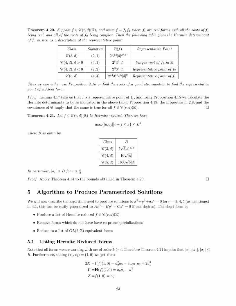
Theorem 4.20. Suppose f ∈ C (r, d)(R), and write f = f1f2 where fi are real forms with all the roots of f1

being real, and all of the roots of f2 being complex. Then the following table gives the Hermite determinant

of f , as well as a description of the representative point:

Class Signature Θ(f) Representative Point

C (3, d) (2, 1) 2633|d|2/3 -

C (4, d), d > 0 (4, 1) 2839|d| Unique root of f2 in H

C (4, d), d < 0 (2, 2) 2839|d| Representative point of f2

C (5, d) (4, 4) 22431855|d|2 Representative point of f1

Thus we can either use Proposition 4.16 or find the roots of a quadratic equation to find the representative

point of a Klein form.

Proof. Lemma 4.17 tells us that i is a representative point of fr, and using Proposition 4.15 we calculate the

Hermite determinants to be as indicated in the above table. Proposition 4.19, the properties in 2.8, and the

covariance of Θ imply that the same is true for all f ∈ C (r, d)(R).

Theorem 4.21. Let f ∈ C (r, d)(R) be Hermite reduced. Then we have

max|aiaj |∣∣i+ j ≤ k ≤ B2

where B is given by

Class B

C (3, d) 2√

3|d|1/3

C (4, d) 16√|d|

C (5, d) 1600√

5|d|

In particular, |ai| ≤ B for i ≤ k2 .

Proof. Apply Theorem 4.14 to the bounds obtained in Theorem 4.20.

5 Algorithm to Produce Parametrized Solutions

We will now describe the algorithm used to produce solutions to x2 +y3 +dzr = 0 for r = 3, 4, 5 (as mentioned

in 4.1, this can be easily generalized to Ax2 +By3 + Czr = 0 if one desires). The short form is:

• Produce a list of Hermite reduced f ∈ C (r, d)(Z)

• Remove forms which do not have have co-prime specializations

• Reduce to a list of GL(2,Z) equivalent forms

5.1 Listing Hermite Reduced Forms

Note that all forms we are working with are of order k ≥ 4. Therefore Theorem 4.21 implies that |a0|, |a1|, |a2| ≤B. Furthermore, taking (z1, z2) = (1, 0) we get that:

2X =t(f)(1, 0) = a20a3 − 3a0a1a2 + 2a3

1

Y =H(f)(1, 0) = a0a2 − a21

Z =f(1, 0) = a0

23

satisfy X2 +Y 3 +dZr = 0. Therefore for each selection of integers a0, a1, a2 in the range [−B,B], we calculate

Y,Z and X = ±√−Y 3 − dZr. If X is not an integer then we get no solution. Otherwise, we have at most 2

choices for X, and we must have the start of a parametrization which specializes to (±X,Y, Z). In the case

a0 6= 0, the equation for X determines a3, and the equations found in Appendix A show that the rest of

the ai are uniquely determined. If a0 = 0 then the defining equations determine the rest of the coefficients

uniquely.

Calculate the representative point using Theorem 4.20 and Proposition 4.16; if it lies in D then we must

have a Hermite reduced form in C (r, d)(Z). Note that if our form has a root at infinity, then before applying

Proposition 4.16 we apply a suitable Mobius map, and then translate the representative point back.

When programming the algorithm, one must be aware of the limitations of floating point arithmetic. When

checking if a point is in the fundamental domain, one should increase the bounds of the domain slightly; for

example, if the representative point z has |z| = 1, the program may calculate |z| as 0.9999999 and then

|z| ≥ 1 would be false. In increasing our tolerance we may also let in a few non-reduced forms, which we will

remove later.

5.2 Coprime Specializations

For r = 3, 4, 5, let N = 12, 24, 60 respectively (the size of the rotation group r corresponds to). Then we have

the following proposition

Proposition 5.1. Let f ∈ C (r, d)(Z) where d 6= 0, and let φ = ( 12t(f),H(f), f). Then if φ has coprime

integer specializations, then there exist (z1, z2) ∈ Z2 such that |zi| ≤ N ′ such that φ(z1, z2) is coprime, where

N ′ is product of all odd primes dividing Nd.

Proof. If f,H(f) have resultant R, then thinking of them as integer polynomials, we have A,B ∈ Z[z1, z2]

such that Af + BH(f) = R. Thus we are done if we show that the primes dividing the resultant of f,H(f)

are the primes dividing Nd.

The resultant can also be thought of as follows: let a(x) = A∏mi=1(x − ai) and b(x) = B

∏ni=1(x − bi).

Then Res(A,B) = AnBm∏

1≤i≤m,1≤j≤n(ai − bj).

Now, we have the form f = [0, 1, 0, 0,−4d] ∈ C (3, d), and we can check the proposition directly for f . We

can do the same with r = 4, 5 by starting with (a0, a1, a2) = (0, 1, 0) and following the defining equations

to get a form f ∈ C (r, d). A general g ∈ C (r, d) is SL(2,C) equivalent to f , and SL(2,C) is generated by(0 1−1 0

)and

(1 λ0 1

)for λ ∈ C. Using the covariance of H(f) and the above definition of resultant, we see that

applying(

1 λ0 1

)does not change the value of the resultant, and applying

(0 1−1 0

)will also not change the value

of the resultant, whence the claim.

5.3 Removing equivalent forms

A list with no GL(2,Z) equivalent forms is a minimal list, as all integer solutions occur as integer special-

izations of an entry on our list, and any two entries give different integer specializations. When working over

GL(2,Z), we add in the matrix(−1 0

0 1

)to the mix which changes the fundamental domain to

D− =

z = x+ iy

∣∣∣∣|z| ≥ 1,−1

2≤ x ≤ 0

.

Furthermore, two distinct forms can only be equivalent when their representative point is on the boundary

of the fundamental domain! Thus we can calculate the stabilizer of each such point and test if our forms are

related by these maps. Edwards does this in [6], and the stabilizer is of size 2 outside of i and ω, the primitive

24

cube root of unity (where the size is now 6, 4 respectively).

This provides a good algorithm, however we will take a slightly different approach. MAGMA has the built

in function “IsGL2Equivalent”, which takes two forms of a specified degree and tests if they are equivalent

over GL(2,K), with K being the base field of the forms. The benefit of this is (as mentioned previously), we

account for rounding errors by potentially including forms which have representative point not quite in the

fundamental domain. Using this function allows us to also rid those forms. This change should increase com-

putation time, however is is minimal as the list of forms we consider is small (the computationally expensive

part is generating the initial list of Hermite reduced forms).

When using “IsGL2Equivalent” we do have to be slightly careful, as it works over Q and not Z. Thus for

each transition matrix we get, we must check that it has determinant ±1 and integer entries.

5.4 Modifying the algorithm for general S

We wish to have something slightly better than the remark following Proposition 4.5, where we said that

we can take f ∈ C (r, d)(ZS). Indeed, assume we are given X,Y, Z with X2 + Y 3 + dZr = 0, and let p be

any prime dividing gcd(X,Y ). If p5 | dZr, then working modulo powers of p we get that p3 | X, p2 | Y , and

p6 | dZ. So we can divide through by p6 to get an equation of the form X21 + Y 3

1 + d1Zr1 = 0 with d

d1being

a power of p. Repeat and we see that we can assume p5 - d′Zr where d′

is some divisor of d with dd′

being a

power of p (there are finitely many such possibilities).

If r = 5 then p - Z, and for r = 3, 4 we have p2 - Z. Thus following Proposition 4.5, when we lift out

integer solution we take a0 = Z, and following through the equations we see that U (f) ⊂ Z if r = 5 and

U (f) ⊂ 1pZ for r = 3, 4. This implies we can continue taking U (f) ⊂ Z if r = 5 (though we need to repeat

for all d′ | d where d

d′only has prime divisors from the set S). As our set S is finite, let P be the product of

the primes in S, and for r = 3, 4 we can take U (f) ⊂ 1P Z. Thus we still have a finite algorithm (coefficients

are bounded with bounded denominators!

Checking that our solutions have specializations where the only primes dividing gcd(X,Y, Z) are in S is

completely analogous to Proposition 5.1, as we only need to consider the resultant of f,H(f).

6 Explicit Calculations and Varying d

We shall give some results of our program, and compare them to the results presented by Edwards in [6].

We will only consider the Tetrahedral and Octahedral cases, as the Icosahedral case is very computationally

demanding. Note that a form f ∈ C (d, r) will be presented as [a0, a1, . . . , ak].

6.1 Tetrahedron

We may as well take d > 0 for the tetrahedron, since −1 being an integral cube implies the cases of d and

−d are analogous. Comparing the case of d = 1 with Edwards’s results on page 233 of [6] we get

25

d = 1

Our Results Representative Point Edwards’s Results

[−2,−1, 0,−1,−2] −0.268 + 0.963i [−2,−1, 0,−1,−2]

[−1, 1, 1, 1,−1] −0.268 + 0.963i [−1, 1, 1, 1,−1]

[−1, 0,−1, 0, 3] 4√

3i [−1, 0,−1, 0, 3]

[1, 0,−1, 0,−3] 4√

3i [1, 0,−1, 0,−3]

[−1, 0, 0,−2, 0]√

2i [−1, 0, 0, 2, 0]

[0, 1, 0, 0,−4]√

2i [0, 1, 0, 0,−4]

We have rearranged them so that they come in pairs with the same representative point. As noted in [6],

X2 +Y 3 +Z3 = 0 is symmetric in Y,Z, and the consecutive pairs correspond to switching (Y,Z) with (Z, Y ).

We next calculate the reduced forms, find the number N of non-equivalent reduced forms for d =

1, 2, . . . , 60, and present this data in a table.

d N d N d N d N d N d N

1 6 11 8 21 4 31 4 41 4 51 4

2 3 12 5 22 3 32 2 42 2 52 6

3 4 13 4 23 4 33 4 43 8 53 12

4 5 14 2 24 8 34 2 44 11 54 6

5 4 15 8 25 8 35 8 45 8 55 12

6 2 16 4 26 9 36 12 46 6 56 6

7 4 17 12 27 6 37 12 47 8 57 8

8 9 18 6 28 11 38 3 48 8 58 4

9 8 19 8 29 4 39 8 49 8 59 4

10 5 20 5 30 3 40 6 50 6 60 6

There are relatively few occurrences of N being odd, and they only occur when d is even. This leads to

the conjecture that if d is odd, then N is even.

We also see that N > 0 for all d, i.e. C (3, d)(Z) is never empty. Inspired by an observation in the Octahedral

case (see Theorem 6.2), we prove the following theorem.

Theorem 6.1. Let d be a non-zero integer, and write |4d| = (pe11 · · · pess )2qf11 · · · qftt where pi, qj are distinct

primes and fj is odd for all j. Let S be the set of integers which are a product of a subset of pe11 , . . . , pess

(the product of the empty set is 1; note that S has size 2s). Let N = |S ∩ [1,√

2 3√d]|, i.e. the number

of elements of S which are positive and at most√

2 3√d. Then there are exactly N non-equivalent forms

f = [a0, a1, . . . , a4] ∈ C (3, d)(Z) such that a0 = a2 = 0. In particular, C (3, d)(Z) is non-empty.

Proof. Following the defining equations we get

f = [0, a, 0, 0,−4d

a2]

26

Thus we get a form for all integers a with a2 | −4d. If b = −4da2 , then we calculate the covariants 1

2t,H to be

1

2t(f)(z1, z2) =a3z6

1 + 5a2bz31z

32 −

ab2

2z6

2

H(f)(z1, z2) =− a2z41 + 2abz1z

32

f(z1, z2) =4az31z2 + bz4

2

As our form needs coprime specializations, we cannot have a prime divide both a and b, else said prime will

divide all of1

2t,H, f . From

(1

2t

)2

+ (H)3 + df3 = 0, coprimality among all three is equivalent to f,H being

coprime.

I claim that if a, b are coprime, then the form has coprime specializations. Indeed, consider taking (z1, z2) =

(1, 1). Then −H(1, 1) = a2 − 2ab = a(a− 2b), and f(1, 1) = 4a+ b. As a, b are coprime, gcd(a, 4a+ b) = 1 so

gcd(−H, f) = gcd(a− 2b, 4a+ b) = gcd(2(4a+ b) + a− 2b, 4a+ b) = gcd(9a, 4a+ b) = gcd(9, 4a+ b).

Thus we are done if 3 - 4a+b. If 3 | 4a+b, then take (z1, z2) = (1,−1) to get −H(1,−1) = a2 +2ab = a(a+2b)

and f(1,−1) = b − 4a. As above, gcd(H, f) = gcd(9, b − 4a). Thus if this is also not 1, 3 | b − 4a whence

3 | (4a+ b) + (b− 4a) = 2b so 3 | b, and so 3 | a, contradicting a, b being coprime.

Next we calculate the representative point of f . WLOG we can take a > 0 and d > 0. We first do

the transformation (z1, z2) → (−z2, z1) to shift away the root at infinity. We are thus left to consider the

roots of z4 − 4ab z = z4 + a3

d z. Letting ω = − 12 +

√3

2 i be a primitive cube root of unity, we have real roots

α1 = 0, α2 = −a3√d

and complex roots β, β with β = −a3√dω.

We have weights

t21 =|β − β||α2 − β|2 =a√

33√d

(a√

33√d

)2

=3√

3a3

d

t22 =|β − β||α1 − β|2 = · · · =√

3a3

d

u21 =|α1 − α2||α1 − β||α2 − β| =

√3a3

d.

So our quadratic form is

g(x) =

√3a3

d

(3x2 +

(x+

a3√d

)2+ 2(x− β)(x− β)

)=

6√

3a3

d

(x2 +

a2

23√d2

),

which has root in the upper half plane of a√2

3√di. Translating back to the equation for f means that f has

representative point √2 3√d

ai.

Thus our form is reduced if and only if a ≤√

2 3√d. Since a, −4d

a2 = b must be coprime, any prime that divides

4d to an odd power must not divide a. Each prime dividing 4d to an even power can either not divide a, or

fully divide a. The theorem thus follows.

Unfortunately we cannot give a simpler statement of N in the above theorem, as the√

2 3√d bound creates

some problems (this will be in contrast to Theorem 6.2, the analogous result for the octahedron, where a

simpler statement does exist). One will need to look at the exact factorization of any given d to determine the

exact behaviour. However we do have a bound on N ; clearly N ≤ 2s where s is as in the problem statement.

This bound is also exact in many cases, for example when d is a prime (or a product of odd powers of primes).

27

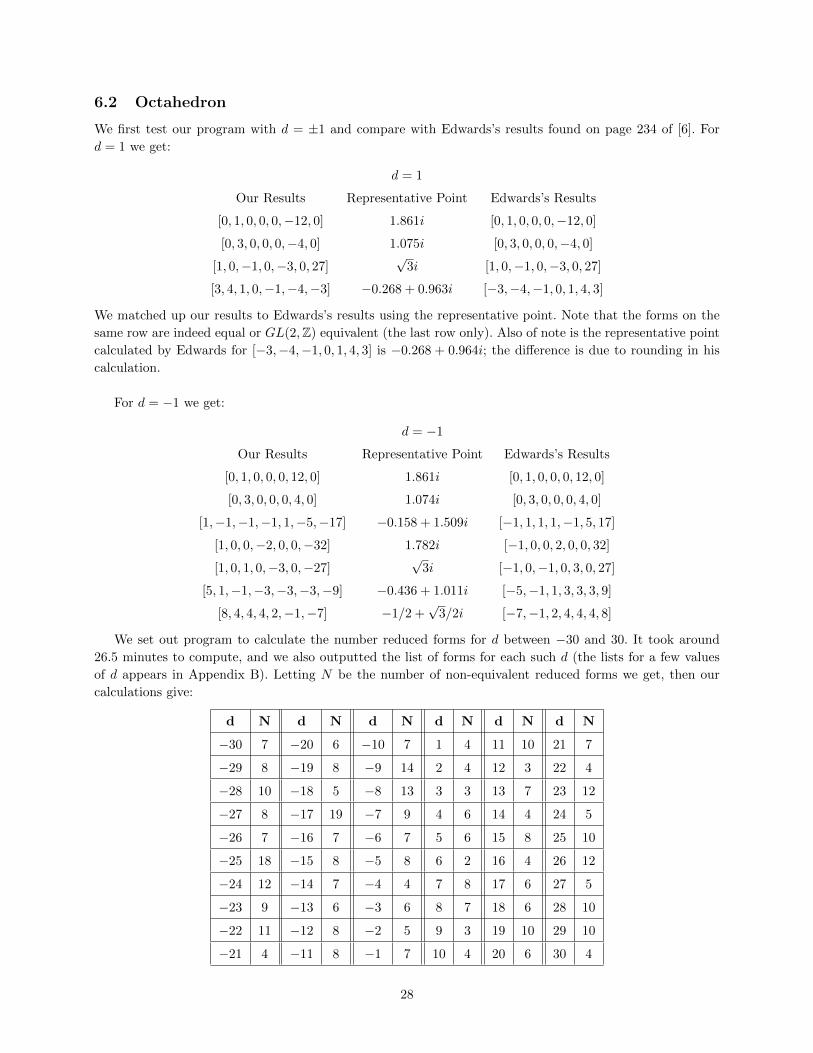
6.2 Octahedron

We first test our program with d = ±1 and compare with Edwards’s results found on page 234 of [6]. For

d = 1 we get:

d = 1

Our Results Representative Point Edwards’s Results

[0, 1, 0, 0, 0,−12, 0] 1.861i [0, 1, 0, 0, 0,−12, 0]

[0, 3, 0, 0, 0,−4, 0] 1.075i [0, 3, 0, 0, 0,−4, 0]

[1, 0,−1, 0,−3, 0, 27]√

3i [1, 0,−1, 0,−3, 0, 27]

[3, 4, 1, 0,−1,−4,−3] −0.268 + 0.963i [−3,−4,−1, 0, 1, 4, 3]

We matched up our results to Edwards’s results using the representative point. Note that the forms on the

same row are indeed equal or GL(2,Z) equivalent (the last row only). Also of note is the representative point

calculated by Edwards for [−3,−4,−1, 0, 1, 4, 3] is −0.268 + 0.964i; the difference is due to rounding in his

calculation.

For d = −1 we get:

d = −1

Our Results Representative Point Edwards’s Results

[0, 1, 0, 0, 0, 12, 0] 1.861i [0, 1, 0, 0, 0, 12, 0]

[0, 3, 0, 0, 0, 4, 0] 1.074i [0, 3, 0, 0, 0, 4, 0]

[1,−1,−1,−1, 1,−5,−17] −0.158 + 1.509i [−1, 1, 1, 1,−1, 5, 17]

[1, 0, 0,−2, 0, 0,−32] 1.782i [−1, 0, 0, 2, 0, 0, 32]

[1, 0, 1, 0,−3, 0,−27]√

3i [−1, 0,−1, 0, 3, 0, 27]

[5, 1,−1,−3,−3,−3,−9] −0.436 + 1.011i [−5,−1, 1, 3, 3, 3, 9]

[8, 4, 4, 4, 2,−1,−7] −1/2 +√

3/2i [−7,−1, 2, 4, 4, 4, 8]

We set out program to calculate the number reduced forms for d between −30 and 30. It took around

26.5 minutes to compute, and we also outputted the list of forms for each such d (the lists for a few values

of d appears in Appendix B). Letting N be the number of non-equivalent reduced forms we get, then our

calculations give:

d N d N d N d N d N d N

−30 7 −20 6 −10 7 1 4 11 10 21 7

−29 8 −19 8 −9 14 2 4 12 3 22 4

−28 10 −18 5 −8 13 3 3 13 7 23 12

−27 8 −17 19 −7 9 4 6 14 4 24 5

−26 7 −16 7 −6 7 5 6 15 8 25 10

−25 18 −15 8 −5 8 6 2 16 4 26 12

−24 12 −14 7 −4 4 7 8 17 6 27 5

−23 9 −13 6 −3 6 8 7 18 6 28 10

−22 11 −12 8 −2 5 9 3 19 10 29 10

−21 4 −11 8 −1 7 10 4 20 6 30 4

28

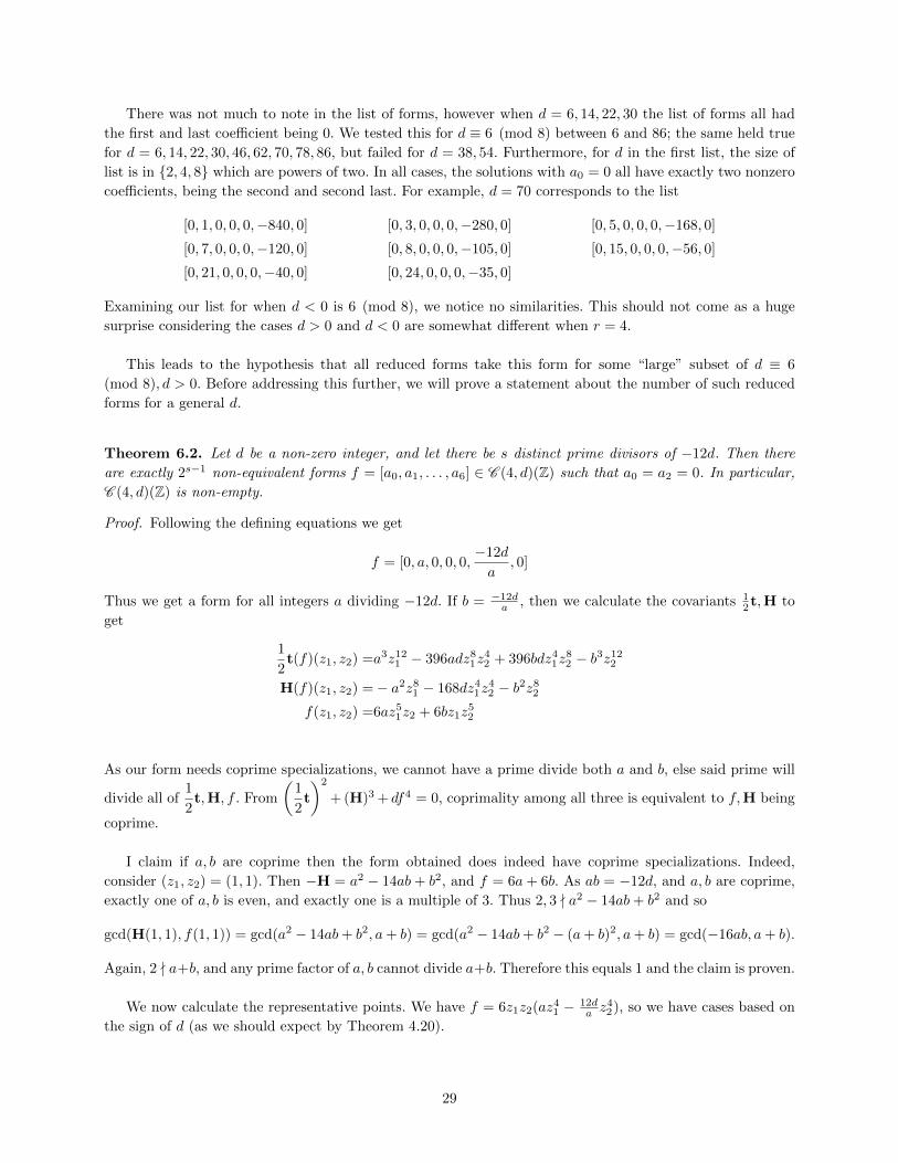
There was not much to note in the list of forms, however when d = 6, 14, 22, 30 the list of forms all had

the first and last coefficient being 0. We tested this for d ≡ 6 (mod 8) between 6 and 86; the same held true

for d = 6, 14, 22, 30, 46, 62, 70, 78, 86, but failed for d = 38, 54. Furthermore, for d in the first list, the size of

list is in 2, 4, 8 which are powers of two. In all cases, the solutions with a0 = 0 all have exactly two nonzero

coefficients, being the second and second last. For example, d = 70 corresponds to the list

[0, 1, 0, 0, 0,−840, 0] [0, 3, 0, 0, 0,−280, 0] [0, 5, 0, 0, 0,−168, 0]

[0, 7, 0, 0, 0,−120, 0] [0, 8, 0, 0, 0,−105, 0] [0, 15, 0, 0, 0,−56, 0]

[0, 21, 0, 0, 0,−40, 0] [0, 24, 0, 0, 0,−35, 0]

Examining our list for when d < 0 is 6 (mod 8), we notice no similarities. This should not come as a huge

surprise considering the cases d > 0 and d < 0 are somewhat different when r = 4.

This leads to the hypothesis that all reduced forms take this form for some “large” subset of d ≡ 6

(mod 8), d > 0. Before addressing this further, we will prove a statement about the number of such reduced

forms for a general d.

Theorem 6.2. Let d be a non-zero integer, and let there be s distinct prime divisors of −12d. Then there

are exactly 2s−1 non-equivalent forms f = [a0, a1, . . . , a6] ∈ C (4, d)(Z) such that a0 = a2 = 0. In particular,

C (4, d)(Z) is non-empty.

Proof. Following the defining equations we get

f = [0, a, 0, 0, 0,−12d

a, 0]

Thus we get a form for all integers a dividing −12d. If b = −12da , then we calculate the covariants 1

2t,H to

get

1

2t(f)(z1, z2) =a3z12

1 − 396adz81z

42 + 396bdz4

1z82 − b3z12

2

H(f)(z1, z2) =− a2z81 − 168dz4

1z42 − b2z8

2

f(z1, z2) =6az51z2 + 6bz1z

52

As our form needs coprime specializations, we cannot have a prime divide both a and b, else said prime will

divide all of1

2t,H, f . From

(1

2t

)2

+ (H)3 + df4 = 0, coprimality among all three is equivalent to f,H being

coprime.

I claim if a, b are coprime then the form obtained does indeed have coprime specializations. Indeed,

consider (z1, z2) = (1, 1). Then −H = a2 − 14ab+ b2, and f = 6a+ 6b. As ab = −12d, and a, b are coprime,

exactly one of a, b is even, and exactly one is a multiple of 3. Thus 2, 3 - a2 − 14ab+ b2 and so

gcd(H(1, 1), f(1, 1)) = gcd(a2 − 14ab+ b2, a+ b) = gcd(a2 − 14ab+ b2 − (a+ b)2, a+ b) = gcd(−16ab, a+ b).

Again, 2 - a+b, and any prime factor of a, b cannot divide a+b. Therefore this equals 1 and the claim is proven.

We now calculate the representative points. We have f = 6z1z2(az41 − 12d

a z42), so we have cases based on

the sign of d (as we should expect by Theorem 4.20).

29

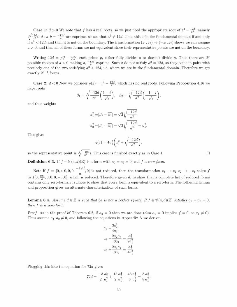
Case 1: d > 0 We note that f has 4 real roots, so we just need the appropriate root of z4 − 12da2 , namely

4

√12da2 i. As a, b = −12d

a are coprime, we see that a2 6= 12d. Thus this is in the fundamental domain if and only

if a2 < 12d, and then it is not on the boundary. The transformation (z1, z2)→ (−z1, z2) shows we can assume

a > 0, and then all of these forms are not equivalent since their representative points are not on the boundary.

Writing 12d = pe11 · · · pess , each prime pi either fully divides a or doesn’t divide a. Thus there are 2s

possible choices of a > 0 making a, −12da coprime. Such a do not satisfy a2 = 12d, so they come in pairs with

precicely one of the two satisfying a2 < 12d, i.e. where we are in the fundamental domain. Therefore we get

exactly 2s−1 forms.

Case 2: d < 0 Now we consider g(z) = z4 − 12da2 , which has no real roots. Following Proposition 4.16 we

have roots

β1 =4

√−12d

a2

(1 + i√

2

), β2 =

4

√−12d

a2

(−1− i√

2

),

and thus weights

u21 =|β2 − β2| =

√2

4

√−12d

a2

u22 =|β1 − β1| =

√2

4

√−12d

a2= u2

1.

This gives

g(z) = 4u21

(z2 +

√−12d

a2

),

so the representative point is 4

√−12da2 i. This case is finished exactly as in Case 1.

Definition 6.3. If f ∈ C (4, d)(Z) is a form with a0 = a2 = 0, call f a zero-form.

Note if f = [0, a, 0, 0, 0,−12d

a, 0] is not reduced, then the transformation z1 → z2, z2 → −z1 takes f

to f [0, 12da , 0, 0, 0,−a, 0], which is reduced. Therefore given d, to show that a complete list of reduced forms

contains only zero-forms, it suffices to show that every form is equivalent to a zero-form. The following lemma

and proposition gives an alternate characterization of such forms.

Lemma 6.4. Assume d ∈ Z is such that 3d is not a perfect square. If f ∈ C (4, d)(Z) satisfies a0 = a6 = 0,

then f is a zero-form.

Proof. As in the proof of Theorem 6.2, if a2 = 0 then we are done (also a1 = 0 implies f = 0, so a1 6= 0).

Thus assume a1, a2 6= 0, and following the equations in Appendix A we derive:

a3 =3a2

2

4a1

a4 =2a2a3

3a1=

a32

2a21

a5 =2a3a4

3a2=

a42

4a31

Plugging this into the equation for 72d gives

72d =−3

2

a42

a21

+15

2

a42

a21

− 45

8

a42

a21

=3

8

a42

a21

,

30

whence (a2

2

a1

)2

= 192d = 263d.

Thus 3d is a perfect square, contradiction.

Note that the above proof still works in many (but not all) cases in which 3d is a perfect square, as then

most resulting forms do not have coprime specializations (for example, if a1 | a2 then the form is always

divisible by a1).

Proposition 6.5. Assume d ∈ Z is such that 3d is not a perfect square. Then f ∈ C (4, d)(Z) is equivalent

to a zero-form if and only if it has at least two roots r1, r2 satisfying either 1) or 2):

1) r1 =∞ and one of r2,1r2

is an integer (and vice versa)

2) r1 = p1q1

and r2 = p2q2

with (p1, q1) = (p2, q2) = 1, and |p1q2 − p2q1| = 1.

Proof. Zero forms have the roots 0,∞, and the forms they are equivalent to are all GL(2,Z) transformations

of themselves. By considering whether 0,∞ go to finite or infinite places, we get that 1) or 2) always holds.

For the only if, we consider doing the if in reverse to transform our form so that it has roots at 0,∞.

Thus a0 = a6 = 0, so by Lemma 6.4 we have a zero-form.

Conjecture 6.6. For a “large” subset of d > 0, d ≡ 6 (mod 8), every form f ∈ C (4, d)(Z) has two roots

satisfying conditions 1) or 2).

Note that if d ≡ 6 (mod 8), then 3d ≡ 2 (mod 4) so it cannot be a perfect square. Thus by our work in

this section, a proof of the conjecture would prove that such d have only zero-forms as reduced forms, and

also that there are exactly 2s−1 equivalence classes of forms, where s is the number of prime divisors of 12d.

7 Further Research

In the tetrahedral case, the phenomenon of the number N of non-equivalent reduced forms being mostly

even (and always even when d is odd) is potentially worth investigating. A possible approach would be: for

every form f ∈ C (3, d)(Z), assign it a “dual form” such that equivalent forms have equivalent dual forms. If

a form is never self-dual, then this would imply that N is even. The fact that any two forms are related by

an element of SL(2,R)+ could potentially lead to a way to assign the dual forms.

For the octahedron, the case of d ≡ 6 (mod 8) and d > 0 is quite interesting: why are all reduced forms

normally zero-forms, and why are there exceptions? An attempt at proving Conjecture 6.6 seems to be the

the most approachable method of doing this. A plausible method would be showing the form has two rational

roots, shifting one to ∞, and then showing that either the numerator or denominator of the remaining root

must be 1.

A Appendix A

The defining equations of the tetrahedron, octahedron, and icosahedron can be obtained by finding algebraic

expressions for τr, τ6, j as seen in Theorem 4.3. One can repeat the calculations using a computer math pack-

age, or by hand if they are feeling rather ambitious. We present the final calculations as given in Edward’s

thesis, [6]. Note that his definition of d differs to ours by a minus sign.

31

For the format, we have

f =

k∑i=0

(k

i

)aiz

k−i1 zi2

τ4(f) =A0z2k−81 + · · ·

τ6(f) =B0z2k−121 + · · ·

The equations we will present are useful when writing a program to do calculations, in which we also

have:

2X =t(f)(1, 0) = a20a3 − 3a0a1a2 + 2a3

1

Y =H(f)(1, 0) = a0a2 − a21

Z =f(1, 0) = a0.

A.1 Tetrahedron

These were presented at just after Theorem 4.3:

0 =a0a4 − 4a1a3 + 3a22

4d =a0a2a4 + 2a1a2a3 − a32 − a0a

23 − a2

1a4.

A.2 Octahedron

The defining equations τ4(f) = 0, τ6(f) = 72d give:

A0/1 : 0 =a0a4 − 4a1a3 + 3a22

A1/2 : 0 =a0a5 − 3a1a4 + 2a2a3

A2/1 : 0 =a0a6 − 9a2a4 + 8a23

A3/2 : 0 =a1a6 − 3a2a5 + 2a3a4

A4/1 : 0 =a2a6 − 4a3a5 + 3a24

B0 : 72d =a0a6 − 6a1a5 + 15a2a4 − 10a23

32

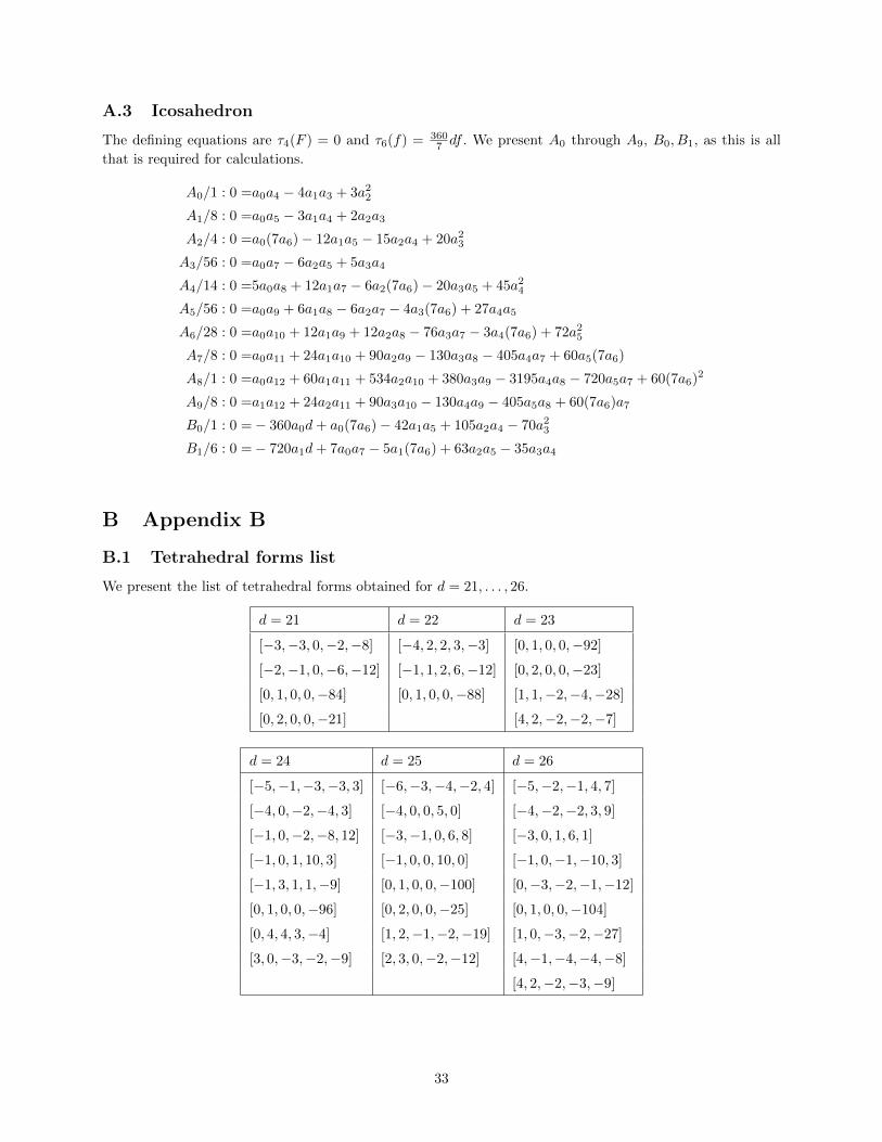
A.3 Icosahedron

The defining equations are τ4(F ) = 0 and τ6(f) = 3607 df . We present A0 through A9, B0, B1, as this is all

that is required for calculations.

A0/1 : 0 =a0a4 − 4a1a3 + 3a22

A1/8 : 0 =a0a5 − 3a1a4 + 2a2a3

A2/4 : 0 =a0(7a6)− 12a1a5 − 15a2a4 + 20a23

A3/56 : 0 =a0a7 − 6a2a5 + 5a3a4

A4/14 : 0 =5a0a8 + 12a1a7 − 6a2(7a6)− 20a3a5 + 45a24

A5/56 : 0 =a0a9 + 6a1a8 − 6a2a7 − 4a3(7a6) + 27a4a5

A6/28 : 0 =a0a10 + 12a1a9 + 12a2a8 − 76a3a7 − 3a4(7a6) + 72a25

A7/8 : 0 =a0a11 + 24a1a10 + 90a2a9 − 130a3a8 − 405a4a7 + 60a5(7a6)

A8/1 : 0 =a0a12 + 60a1a11 + 534a2a10 + 380a3a9 − 3195a4a8 − 720a5a7 + 60(7a6)2

A9/8 : 0 =a1a12 + 24a2a11 + 90a3a10 − 130a4a9 − 405a5a8 + 60(7a6)a7

B0/1 : 0 =− 360a0d+ a0(7a6)− 42a1a5 + 105a2a4 − 70a23

B1/6 : 0 =− 720a1d+ 7a0a7 − 5a1(7a6) + 63a2a5 − 35a3a4

B Appendix B

B.1 Tetrahedral forms list

We present the list of tetrahedral forms obtained for d = 21, . . . , 26.

d = 21 d = 22 d = 23

[−3,−3, 0,−2,−8] [−4, 2, 2, 3,−3] [0, 1, 0, 0,−92]

[−2,−1, 0,−6,−12] [−1, 1, 2, 6,−12] [0, 2, 0, 0,−23]

[0, 1, 0, 0,−84] [0, 1, 0, 0,−88] [1, 1,−2,−4,−28]

[0, 2, 0, 0,−21] [4, 2,−2,−2,−7]

d = 24 d = 25 d = 26

[−5,−1,−3,−3, 3] [−6,−3,−4,−2, 4] [−5,−2,−1, 4, 7]

[−4, 0,−2,−4, 3] [−4, 0, 0, 5, 0] [−4,−2,−2, 3, 9]

[−1, 0,−2,−8, 12] [−3,−1, 0, 6, 8] [−3, 0, 1, 6, 1]

[−1, 0, 1, 10, 3] [−1, 0, 0, 10, 0] [−1, 0,−1,−10, 3]

[−1, 3, 1, 1,−9] [0, 1, 0, 0,−100] [0,−3,−2,−1,−12]

[0, 1, 0, 0,−96] [0, 2, 0, 0,−25] [0, 1, 0, 0,−104]

[0, 4, 4, 3,−4] [1, 2,−1,−2,−19] [1, 0,−3,−2,−27]

[3, 0,−3,−2,−9] [2, 3, 0,−2,−12] [4,−1,−4,−4,−8]

[4, 2,−2,−3,−9]

33

B.2 Octahedral forms list

We present the list of octahedral forms obtained for d = −15,−14,−13, 13, 14, 15.

d = −15 d = −14 d = −13

[0, 1, 0, 0, 0, 180, 0] [0, 1, 0, 0, 0, 168, 0] [0, 1, 0, 0, 0, 156, 0]

[0, 4, 0, 0, 0, 45, 0] [0, 3, 0, 0, 0, 56, 0] [0, 3, 0, 0, 0, 52, 0]

[0, 5, 0, 0, 0, 36, 0] [0, 7, 0, 0, 0, 24, 0] [0, 4, 0, 0, 0, 39, 0]

[0, 8, 8, 6, 4, 25, 69] [0, 8, 0, 0, 0, 21, 0] [0, 12, 0, 0, 0, 13, 0]

[0, 9, 0, 0, 0, 20, 0] [2, 1, 0, 7, 14, 21,−196] [5, 1, 2, 8, 4,−4,−88]

[1,−10,−9,−6,−3,−18,−45] [7, 3, 2,−6,−12,−12,−72] [11, 1,−2,−8,−4,−4,−40]

[1, 0,−1,−8,−3,−16,−485] [9, 3, 6, 6,−4,−12,−56]

[21, 4, 7, 0,−7,−4,−21]

d = 13 d = 14 d = 15

[0, 1, 0, 0, 0,−156, 0] [0, 1, 0, 0, 0,−168, 0] [0, 1, 0, 0, 0,−180, 0]

[0, 3, 0, 0, 0,−52, 0] [0, 3, 0, 0, 0,−56, 0] [0, 4, 0, 0, 0,−45, 0]

[0, 4, 0, 0, 0,−39, 0] [0, 7, 0, 0, 0,−24, 0] [0, 5, 0, 0, 0,−36, 0]

[0, 8, 8, 6, 4,−17,−57] [0, 8, 0, 0, 0,−21, 0] [0, 9, 0, 0, 0,−20, 0]

[0, 12, 0, 0, 0,−13, 0] [1,−1,−3,−3,−15, 27, 333]

[1, 4,−1, 0,−3,−36, 27] [5,−2,−6,−6,−12, 0, 72]

[15, 16, 5, 0,−5,−16,−15] [9, 0,−6,−6,−12,−8, 40]

[9, 18, 12, 6, 0,−16,−32]

References

[1] F. Beukers, The Diophantine equation Axp +Byq = Czr, Duke Math. J. 91 (1998), no. 1, 61− 88.

[2] B. Bollobas, Linear Analysis, Cambridge University Press, 1990.

[3] H. Darmon and A. Granville, On the equations zm = F (x, y) and Axp +Byq = Czr, Bull. London Math.

Soc. 27 (1995), no. 6, 513− 543.

[4] C. Hermite, Note sur la reduction des fonctions homogenes a coefficients entiers et a deux indeterminees,

J. reine agnew. Math. 36 (1848)

[5] D. Hilbert, Theory of algebraic invariants, Cambridge University Press, 1993 (translation of lecture notes

from 1897).

[6] J. Edwards, A complete solution to X2 + Y 3 + Z5 = 0, J. reine angew. Math. 571 (2004), 213− 236.

[7] J. Edwards (2005). Platonic Solids and Solutions to X2 + Y 3 = dZr (Doctoral dissertation). Retrieved

from http://dspace.library.uu.nl/bitstream/handle/1874/7696/?sequence=24

[8] Felix Klein, Lectures on the icosahedron and the solution of equations of the fifth degree, Kegan Paul,

Trench, Trubner & Co. Ltd., London, 1913 (translation of original 1884 edition)

[9] M. Stoll and J.E. Cremona, On the reduction theory of binary forms, J. reine angew. Math. 565 (2003),

79− 99.

34