Parametric Portfolio Policies: ExploitingCharacteristics in the Cross-Section of EquityReturns

Michael W. BrandtFuqua School of Business, Duke University, and NBER

Pedro Santa-ClaraUCLA Anderson School, Universidade Nova de Lisboa, and NBER

Rossen ValkanovRady School, UCSD

We propose a novel approach to optimizing portfolios with large numbers of assets. Wemodel directly the portfolio weight in each asset as a function of the asset’s characteristics.The coefficients of this function are found by optimizing the investor’s average utilityof the portfolio’s return over the sample period. Our approach is computationally simpleand easily modified and extended to capture the effect of transaction costs, for example,produces sensible portfolio weights, and offers robust performance in and out of sample. Incontrast, the traditional approach of first modeling the joint distribution of returns and thensolving for the corresponding optimal portfolio weights is not only difficult to implementfor a large number of assets but also yields notoriously noisy and unstable results. Wepresent an empirical implementation for the universe of all stocks in the CRSP–Compustatdata set, exploiting the size, value, and momentum anomalies. (JEL G11, G12)

Stock characteristics, such as the firm’s market capitalization, book-to-marketratio, or lagged return, are related to the stock’s expected return, variance,and covariance with other stocks.1 However, exploiting this fact in portfolio

We thank an anonymous referee, Michael Brennan, Kent Daniel, Rob Engle, Larry Harris, Joel Hasbrouck (theeditor), Ravi Jagannathan, Ken Kroner, Bruce Lehmann, Francis Longstaff, Anthony Lynch, Richard Roll,Avanidhar Subrahmanyam, Alan Timmerman, Raman Uppal, Halbert White, and seminar participants atColumbia, CUNY Baruch, Emory, HEC Lausanne, INSEAD, LBS, LSE, NYU, Rochester, Tulane, UCSD,UNC, Universidade Nova de Lisboa, Universidade Catolica Portuguesa, University College Dublin, University ofMichigan, Tilburg, USC, Vienna, the Chicago Quantitative Alliance, the Innovations in Financial EconometricsConference in Honor of the 2003 Nobel at NYU, the Conference in Honor of Jan Mossin at the NorwegianSchool of Economics, the Gutmann Public Lecture, the Los Angeles Quantitative Investment Association,Barclays Global Investors, Mellon Capital, Nomura, the Society of Quantitative Analysts, and Wells CapitalManagement for their comments and suggestions. Send correspondence to Michael W. Brandt, Fuqua Schoolof Business, Duke University, 1 Towerview Drive, Durham, NC 27708; telephone: (919) 660-1948; fax: (919)882-9157. E-mail: mbrandt@duke.edu.

1 Fama and French (1996) find that these three characteristics robustly describe the cross-section of expectedreturns. Chan, Karceski, and Lakonishok (1998) show that these characteristics are also related to the variancesand covariances of returns.

C© The Author 2009. Published by Oxford University Press on behalf of The Society for Financial Studies.All rights reserved. For Permissions, please e-mail: journals.permissions@oxfordjournals.org.doi:10.1093/rfs/hhp003

RFS Advance Access published February 13, 2009

The Review of Financial Studies

management has been, up to now, extremely difficult. The traditional mean–variance approach of Markowitz (1952) requires modeling the expected returns,variances, and covariances of all stocks as functions of their characteristics.This is not only a formidable econometric problem given the large numberof moments involved and the need to ensure the positive definiteness of thecovariance matrix, but the results of the procedure are also notoriously noisyand unstable (e.g., Michaud 1989). In practice, the Markowitz approach istherefore implemented along with a number of different fixes, including shrink-age of the estimates, imposing a factor structure on the covariance matrix,estimation of expected returns from an asset pricing model, or constrainingthe portfolio weights.2 While these fixes generally improve the properties ofthe optimized portfolio, they require substantial resources, such as the toolsdeveloped by BARRA, Northfield, and other companies. As a result, formalportfolio optimization based on firm characteristics is seldom implemented byasset managers (with the notable exception of quant managers, who are a smallpart of the profession), even though it has the potential to provide large benefitsto investors.3

We propose a simple new approach to equity portfolio optimization basedon firm characteristics. We parameterize the portfolio weight of each stockas a function of the firm’s characteristics and estimate the coefficients of theportfolio policy by maximizing the average utility the investor would haveobtained by implementing the policy over the historical sample period.

Our approach has a number of conceptual advantages. First, we avoid com-pletely the auxiliary, yet very difficult, step of modeling the joint distribution ofreturns and characteristics and instead focus directly on the object of interest—the portfolio weights. Second, parameterizing the portfolio policy leads to atremendous reduction in dimensionality. For a problem with N stocks, the tradi-tional Markowitz approach requires modeling N first and (N 2 + N )/2 secondmoments of returns. With preferences other than the simplistic quadratic util-ity, the traditional approach involves a practically unmanageable number ofhigher moments for even a relatively small number of stocks (e.g., 100 stockshave over 300,000 third moments). In contrast, our approach involves model-ing only N portfolio weights regardless of the investor’s preferences and thejoint distribution of asset returns. Because of this reduction in dimensionality,our approach escapes the common statistical problems of imprecise coefficientestimates and overfitting, while allowing us to solve very large-scale problemswith arbitrary preferences. Third, but related, our approach captures implic-itly the relation between the characteristics and expected returns, variances,covariances, and even higher-order moments of returns since they affect the

2 See Jobson and Korkie (1980, 1981); Frost and Savarino (1986, 1988); Jorion (1986); Black and Litterman (1992);Chan, Karceski, and Lakonishok (1999); Pastor (2000); Pastor and Stambaugh (2000, 2002); Jagannathan andMa (2002); and Ledoit and Wolf (2003, 2004). Brandt (2004) surveys the literature.

3 See, for instance, Chan, Karceski, and Lakonishok (1999) and Jagannathan and Ma (2002).

2

Parametric Portfolio Policies

distribution of the optimized portfolio’s returns, and therefore the investor’sexpected utility. Fourth, by framing the portfolio optimization as a statisticalestimation problem with an expected utility objective function (a “maximumexpected utility” estimator as opposed to the usual least-squares or maximum-likelihood estimators), we can easily test individual and joint hypotheses aboutthe optimal portfolio weights.

From a practical perspective, our approach is simple to implement and pro-duces robust results in and out of sample. It is also easily modified and extended.We discuss a number of possible extensions, including the use of different ob-jective functions, the use of different parameterizations of the portfolio policyto accommodate short-sale constraints, and conditioning the portfolio policyon macroeconomic predictors. Perhaps most interestingly, from a practical per-spective, we show how our approach can be extended to capture the effect oftransaction costs.

Our paper is related to a recent literature on drawing inferences about optimalportfolio weights without explicitly modeling the underlying return distribu-tion. Brandt (1999) and Aıt-Sahalia and Brandt (2001) model the optimalallocations to stocks, bonds, and cash as nonparametric functions of variablesthat predict returns. Nigmatullin (2003) extends their nonparametric approachto incorporate parameter and model uncertainty in a Bayesian setting. Moreclosely related to our paper are Brandt and Santa-Clara (2006), who study amarket-timing problem involving stocks, bonds, and cash by modeling the op-timal portfolio weights as functions of the predictors. Specifically, they modelthe weight in each asset class as a separate function (with coefficients that arespecific to the asset class) of a common set of macroeconomic variables. Theirapproach is relevant for problems involving a few assets that have fundamen-tally different characteristics, such as the allocation of capital across differentasset classes. In contrast, our paper models the weight invested in each asset asthe same function (with common coefficients) of asset-specific variables. Thisis the relevant problem when choosing among a large number of essentiallysimilar assets, such as the universe of stocks.

We use our approach to optimize a portfolio of all the stocks in the CRSP-Compustat data set from 1974 to 2002, using as characteristics the market cap-italization, book-to-market ratio, and lagged one-year return of each firm. Theinvestor is assumed to have constant relative risk aversion (CRRA) preferences.Our empirical results document the importance of the firm characteristics forexplaining deviations of the optimal portfolio weights from observed marketcapitalization weights. Relative to market cap weights, the optimal portfoliowith and without short-sale constraints allocates considerably more wealth tostocks of small firms, firms with high book-to-market ratios (value firms), andfirms with high lagged returns (winners). With a relative risk aversion of five,the certainty-equivalent gain from investing in the optimal portfolio relative toholding the market is an annualized 11.1% in sample and 5.4% out of sample.The benefits are even greater when we allow the coefficients of the portfolio

3

The Review of Financial Studies

policy to depend on the slope of the yield curve. We present results for long-only portfolio policies and find that the constraint has significant costs for theinvestor. We examine the impact of increasing the level of risk aversion onthe portfolio policy and find essentially that size and momentum become lessappealing while value retains its importance. Finally, we incorporate transac-tion costs. We show that, with a simple policy function that features a no-tradeboundary, the portfolio turnover is reduced by up to 50% with only marginaldeterioration in performance.

The remainder of the paper proceeds as follows. We describe the basic ideaand various extensions of our approach in Section 1. The empirical applicationis presented in Section 2. We conclude in Section 3.

1. Methodology

1.1 Basic ideaSuppose that at each date t , there is a large number, Nt , of stocks in theinvestable universe.4 Each stock i has a return of ri,t+1 from date t to t + 1and is associated with a vector of firm characteristics xi,t observed at date t .For example, the characteristics could be the market capitalization of the stock,the book-to-market ratio of the stock, and the lagged twelve-month return onthe stock. The investor’s problem is to choose the portfolio weights wi,t tomaximize the conditional expected utility of the portfolio’s return rp,t+1,

max{wi,t }Nt

i=1

Et [u(rp,t+1)] = Et

[u

(Nt∑

i=1

wi,t ri,t+1

)]. (1)

We parameterize the optimal portfolio weights as a function of the stocks’characteristics,

wi,t = f (xi,t ; θ). (2)

In a large part of the paper, we concentrate on the following simple linearspecification for the portfolio weight function:

wi,t = wi,t + 1

Ntθ� xi,t , (3)

where wi,t is the weight of stock i at date t in a benchmark portfolio, such as thevalue-weighted market portfolio, θ is a vector of coefficients to be estimated,and xi,t are the characteristics of stock i , standardized cross-sectionally to havezero mean and unit standard deviation across all stocks at date t . Note that,rather than estimating one weight for each stock at each point in time, we

4 Our method automatically accommodates the realistic case of a varying number of stocks through time. This isnot trivially done in the traditional approach, as discussed by Stambaugh (1997).

4

Parametric Portfolio Policies

estimate weights as a single function of characteristics that applies to all stocksover time—a portfolio policy.

This particular parameterization captures the idea of active portfolio man-agement relative to a performance benchmark. The intercept is the weight ofthe stock in the benchmark portfolio, and the term θ� xi,t represents the devia-tions of the optimal portfolio weight from this benchmark. The characteristicsare standardized for two reasons. First, the cross-sectional distribution of thestandardized xi,t is stationary through time, while that of the raw xi,t maybe nonstationary. Second, the standardization implies that the cross-sectionalaverage of θ� xi,t is zero, which means that the deviations of the optimal port-folio weights from the benchmark weights sum to zero, and therefore that theoptimal portfolio weights always sum to one. Finally, the term 1/Nt is a nor-malization that allows the portfolio weight function to be applied to an arbitraryand time-varying number of stocks. Without this normalization, doubling thenumber of stocks without otherwise changing the cross-sectional distributionof the characteristics results in twice as aggressive allocations, even though theinvestment opportunities are fundamentally unchanged.

There are a number of alternative ways to normalize the firm characteris-tics. One alternative is to subtract the mean characteristic of the industry (at agiven level of aggregation) rather than the mean of the universe. In this way,the standardized characteristics measure deviations from the industry, whichmay clean out systematic operational or financial differences across industries.Asness, Porter, and Steven (2001) stress the importance of industry normal-izations. Besides the impact of purifying the signal for expected returns, usingindustry-normalized characteristics is likely to reduce the risk of the portfoliosince there will be lower net exposure to industries. Another alternative is to runa cross-sectional regression each period of each given characteristic on otherfirm variables (possibly including industry dummies), and take the residuals ofthat regression as inputs to the portfolio policy. These residuals are the com-ponent of the characteristic that is orthogonal to the regression’s explanatoryvariables and will therefore remove all commonality in the characteristics dueto those variables.

The most important aspect of our parameterization is that the coefficientsθ are constant across assets and through time. Constant coefficients across assetsimplies that the portfolio weight in each stock depends only on the stock’scharacteristics and not on the stock’s historic returns. Two stocks that are closeto each other in characteristics associated with expected returns and risk shouldhave similar weights in the portfolio even if their sample returns are verydifferent. The implicit assumption is that the characteristics fully capture allaspects of the joint distribution of returns that are relevant for forming optimalportfolios. Constant coefficients through time means that the coefficients thatmaximize the investor’s conditional expected utility at a given date are the samefor all dates, and therefore also maximize the investor’s unconditional expectedutility.

5

The Review of Financial Studies

These two facts imply that we can rewrite the conditional optimizationwith respect to the portfolio weights wi,t in Equation (1) as the followingunconditional optimization with respect to the coefficients θ:

maxθ

E[u(rp,t+1)] = E

[u

(Nt∑

i=1

f (xi,t ; θ)ri,t+1

)]. (4)

We can then estimate the coefficients θ by maximizing the correspondingsample analog

maxθ

1

T

T −1∑t=0

u(rp,t+1) = 1

T

T −1∑t=0

u

(Nt∑

i=1

f (xi,t ; θ)ri,t+1

), (5)

for some prespecified utility function (e.g., quadratic or CRRA). In the linearpolicy case (3), the optimization problem is

maxθ

1

T

T −1∑t=0

u

(Nt∑

i=1

(wi,t + 1

Ntθ� xi,t

)ri,t+1

). (6)

Four observations about our approach are worth making at this point. First,optimizing a portfolio of a very large number of stocks is extremely simple.Given the relatively low dimensionality of the parameter vector, it is computa-tionally trivial to optimize the portfolio with nonlinear optimization methods.5

The computational burden of our approach only grows with the number ofcharacteristics entering the portfolio policy, not with the number of assets inthe portfolio. Second, the formulation is numerically robust. We optimize theentire portfolio by choosing only a few parameters θ. This parsimony reducesthe risk of in-sample overfitting since the coefficients will only deviate fromzero if the respective characteristics offer an interesting combination of returnand risk consistently across stocks and through time. For the same reason, theoptimized portfolio weights tend not to take extreme values.

Third, the linear policy (3) conveniently nests the long–short portfolios con-struction of Fama and French (1993) or its extension in Carhart (1997). Tosee how this is the case, assume that the portfolio policy in Equation (2) isparameterized in a linear manner as in (3). Let the benchmark weights be themarket capitalization weights and the characteristics be defined as 1 if the stockis in a top quantile, −1 if it is in the bottom quantile, and zero for intermediatequantiles of market capitalization (me), book to market ratio (btm), and past

5 For most common utility functions and given the linearity of the portfolio policy (3) in the coefficients θ, it iseasy to derive analytically the gradient and the Hessian of the optimization problem.

6

Parametric Portfolio Policies

return (mom). Then, the portfolio return is

rp,t+1 = rm,t+1 + θme

Nt∑i=1

(1

Qtmei,t

)ri,t+1 + · · · θbtm

Nt∑i=1

(1

Qtbtmi,t

)ri,t+1

+ θmom

Nt∑i=1

(1

Qtmomi,t

)ri,t+1

= rm,t+1 + θmersmb,t+1 + θbtmrhml,t+1 + θmomrwml,t+1, (7)

where rsmb,t+1, rhml,t+1, and rwml,t+1 are the returns to “small-minus-big,”“high-minus-low,” and “winners-minus-losers” portfolios, and Qt is the numberof firms in the quantile. Under this interpretation, the theta coefficients are theweights put on each of the factor portfolios. To find the weight of the portfolioin each individual stock, we still need to multiply the coefficients θ by therespective characteristics.

While our approach nests the problem of optimally investing in factor-mimicking long–short portfolios, the reverse is only true when the portfoliopolicy is linear and unconstrained. In the more general and practically rele-vant case of constrained portfolio weights, such as the long-only specificationdiscussed in Section 1.3.2, the optimal portfolio can no longer be seen as achoice among long–short factor portfolios. The reason is that with long–shortfactor portfolios, the overall portfolio constraints cannot be imposed on a stock-by-stock basis. Similarly, the portfolio policy proposed in Section 1.4 to dealwith transaction costs is nonlinear and recursive. That policy also cannot beimplemented by a static choice of long–short factor portfolios.

Fourth, the optimization takes into account the relation between the char-acteristics and expected returns, variances, covariances, and even higher-ordermoments of returns, to the extent that they affect the distribution of the opti-mized portfolio’s returns, and therefore the investor’s expected utility. In theoptimization, the degree of cross-sectional predictability of each component ofthe joint return distribution is intuitively weighted by its impact on the overallexpected utility of the investor.

To better understand this point, we can approximate the expected utility ofthe investor with a Taylor series expansion around the portfolio’s expectedreturn E[rp,t+1],

E[u(rp,t+1)] ≈ u(E[rp,t+1]) + 1

2u′′(E[rp,t+1])E[(rp,t+1 − E[rp,t+1])2]

+ 1

6u′′′(E[rp,t+1])E[(rp,t+1 − E[rp,t+1])3] + · · · . (8)

7

The Review of Financial Studies

This expansion shows that, in general, the investor cares about all the momentsof the distribution of the portfolio return.6 Since the portfolio return is given by

rp,t+1 =Nt∑

i=1

f (xi,t ; θ)ri,t+1, (9)

the moments of its distribution depend implicitly on the joint distribution of thereturns and characteristics of all firms. The coefficients θ affect the distributionof the portfolio’s return by changing the weights given to the returns of theindividual firms in the overall portfolio.

To perform a comparable portfolio optimization using the traditionalMarkowitz approach requires modeling the means, variances, and covariancesof all the stocks as functions of their characteristics. This entails estimating foreach date t a large number of Nt conditional expected returns and (N 2

t + Nt )/2conditional variances and covariances. Besides the fact that the number of thesemoments grows quickly with the number of stocks, making robust estimationa real problem, it is extremely challenging to estimate the covariance matrix asa function of stock characteristics in a way that guarantees its positive definite-ness. Furthermore, extending the traditional approach beyond first and secondmoments, when the investor’s utility function is not quadratic, is practicallyimpossible because it requires modeling not only the conditional skewness andkurtosis of each stock but also the numerous high-order cross-moments.

Finally, when the benchmark is the value-weighted market, m, the return ofthe linear portfolio policy (3) can be written as

rp,t+1 =Nt∑

i=1

wi,t ri,t+1 +Nt∑

i=1

(1

Ntθ� xi,t

)ri,t+1 = rm,t+1 + rh,t+1, (10)

where h is a long–short hedge fund with weights θ� xi,t/Nt that add up to zero.Therefore, problem (8) can be reinterpreted as the problem of a hedge fund thatoptimizes its portfolio to maximize the utility of an investor who already holdsthe market (i.e., the market is a background risk for the investor).

1.2 Statistical inferenceBy formulating the portfolio problem as a statistical estimation problem, wecan easily obtain standard errors for the coefficients of the weight function. The“maximum expected utility” estimate θ, defined by the optimization problem

6 This is especially important in dealing with assets with distributions that significantly depart from normality, suchas options and credit-sensitive securities. Santa-Clara and Saretto (2006) provide an application of our approachto option portfolios.

8

Parametric Portfolio Policies

(5) with the linear portfolio policy (3), satisfies the first-order conditions7

1

T

T −1∑t=0

h(rt+1, xt ; θ) ≡ 1

T

T −1∑t=0

u′(rp,t+1)

(1

Ntx�

t rt+1

)= 0, (11)

and can, therefore, be interpreted as a method of moments estimator. FromHansen (1982), the asymptotic covariance matrix of this estimator is

�θ ≡ AsyVar[θ] = 1

T[G�V −1G]−1, (12)

where

G ≡ 1

T

T −1∑t=0

∂h(rt+1, xt ; θ)

∂θ= 1

T

T −1∑t=0

u′′(rp,t+1)

(1

Ntx�

t rt+1

)(1

Ntx�

t rt+1

)�

(13)

and V is a consistent estimator of the covariance matrix of h(r, x ; θ).Assuming marginal utilities are uncorrelated, which is true by construction

when the portfolio policy is correctly specified and the optimization is uncon-strained, we can consistently estimate V by

1

T

T −1∑t=0

h(rt+1, xt ; θ)h(rt+1, xt ; θ)�. (14)

If we want to allow for the possibility of a misspecified portfolio policy (e.g.,for the purpose of specification testing discussed below), or if constraints areimposed, we may instead use an autocorrelation-adjusted estimator of V (e.g.,Newey and West 1987).

Alternatively, the covariance matrix of coefficients �θ can be estimated bybootstrap. For that, we simply generate a large number of samples of returnsand characteristics by randomly drawing monthly observations from the orig-inal data set (with replacement).8 For each of these bootstrapped samples, weestimate the coefficients of the optimal portfolio policy and compute the co-variance matrix of the coefficients across all the bootstrapped samples. Thisapproach has the advantage of not relying on asymptotic results, and takes intoaccount the potentially nonnormal features of the data. We use bootstrappedstandard errors in the empirical analysis below.

The resulting estimate of the covariance matrix of the coefficients �θ can beused to test individual and joint hypotheses about the elements of θ. These testsaddress the economic question of whether a given characteristic is related to the

7 With more general portfolio policies, we also need to differentiate f (xi,t ; θ) with respect to θ.

8 We also experimented with block bootstrapping techniques that maintain the time-series dependence of the data(e.g., Politis and Romano 1994). The resulting inferences are qualitatively the same.

9

The Review of Financial Studies

moments of returns in such a way that the investor finds it optimal to deviatefrom the benchmark portfolio weights according to the realization of the char-acteristic for each stock. It is important to recognize that this is not equivalentto testing whether a characteristic is cross-sectionally related to the conditionalmoments of stock returns for at least two reasons. First, the benchmark portfo-lio weights may already reflect an exposure to the characteristics, and it maynot be optimal to change that exposure. Second, a given characteristic may becorrelated with first and second moments in an offsetting way, such that theconditionally optimal portfolio weights are independent of the characteristic.

The interpretation of our approach as a method of moments estimator sug-gests a way of testing the functional specification of the portfolio policy. Ingoing from Equation (1) to Equation (4), we assume that the functional formof the portfolio policy is correct, to replace wi,t with a function of xi,t , and thatthe coefficients are constant through time, to condition down the expectation.If either assumption is incorrect, the marginal utilities in Equation (11) will becorrelated with variables in the investor’s information set at date t , which mayinclude missing characteristics or variables that are correlated with the variationin the coefficients. We can therefore perform specification tests for the portfoliopolicy using the standard overidentifying restrictions test of Hansen (1982).

Finally, note that the method of moments interpretation does not necessarilyrender our approach frequentist and therefore unable to accommodate finite-sample uncertainty about the parameters and model specification. Nigmatullin(2003) shows how to interpret first-order conditions similar to Equation (11)from a Bayesian perspective using the idea of an empirical likelihood functionand explains how to incorporate parameter and model uncertainty. While hisapplication deals with the nonparametric approach of Aıt-Sahalia and Brandt(2001), the general idea applies directly to our approach.

1.3 Refinements and extensionsBesides its effectiveness and simplicity, an important strength of our approachis that the basic idea is easily refined and extended to suit specific applications.We now discuss some of the possible refinements and extensions to illustratethe flexibility of our approach.

1.3.1 Objective functions. The most important ingredient of any portfoliochoice problem is the investor’s objective function. In contrast to the traditionalMarkowitz approach, our specification of the portfolio choice problem can ac-commodate any choice of objective function. The only implicit assumption isthat the conditional expected utility maximization problem (1) be well spec-ified with a unique solution. Besides the standard HARA preferences (whichnest constant relative risk aversion, constant absolute risk aversion, log, andquadratic utility), our approach can also be applied to behaviorally motivatedutility functions, such as loss aversion, ambiguity aversion, or disappoint-ment aversion, as well as practitioner-oriented objective functions, including

10

Parametric Portfolio Policies

maximizing the Sharpe or information ratios, beating or tracking a benchmark,controlling drawdowns, or maintaining a certain value at risk (VaR).9

In most of the empirical applications, we use standard CRRA preferencesover wealth,

u(rp,t+1) = (1 + rp,t+1)1−γ

1 − γ. (15)

The advantage of CRRA utility is that it incorporates preferences toward higher-order moments in a parsimonious manner. In addition, the utility function istwice continuously differentiable, which allows us to use more efficient numer-ical optimization algorithms that make use of the analytic gradient and Hessianof the objective function. We also offer results for the minimum variance andmaximum Sharpe ratio portfolios.

1.3.2 Portfolio weight constraints. By far the most common departure fromthe basic portfolio choice problem (1) in practice is to impose constraints onthe optimal portfolio weights. In our approach, these constraints have to beimposed through the parameterization of the portfolio policy. For example,consider the case of the no-short-sale constraint in long-only equity portfolios.The simplest way to impose this constraint through the portfolio policy is totruncate the portfolio weights in Equation (3) at zero. Unfortunately, in doingso, the optimal portfolio weights no longer sum to one (setting the negativeweights to zero results in a sum of weights greater than one). We, therefore,need to renormalize the portfolio weights as follows:

w+i,t = max[0, wi,t ]∑Nt

j=1 max[0, w j,t ]. (16)

Besides guaranteeing positivity of the portfolio weights, this specification isalso an example of a nonlinear parameterization of the portfolio weight func-tion (2).

One computational problem with this specification of the portfolio policyfunction is its nondifferentiability at wi,t = 0. In order to compute the standarderrors of the estimated θ from first-order conditions analogous to Equation (11),we require first-order derivatives. One way to overcome this problem in practiceis to approximate the function max[0, y] between two close points y = 0 andy = α > 0 with either a third- or a fifth-order polynomial with smooth first-or first- and second-order derivatives at the end points, respectively. Usingbootstrapped standard errors is an obvious approach to avoid the problem.

9 Benartzi and Thaler (1995); Aıt-Sahalia and Brandt (2001); Ang, Bekaert, and Liu (2005); and Gomes (2005),among others, examine the role of behaviorally motivated preference in portfolio choice. Practitioner-orientedobjective functions are considered, for example, by Roy (1952); Grossman and Vila (1989); Browne (1999);Basak and Shapiro (2001); Tepla (2001); and Alexander and Baptista (2002).

11

The Review of Financial Studies

1.3.3 Nonlinearities and interactions. Although we explicitly specified theportfolio policy (3) as a linear function of the characteristics, the linearityassumption is actually innocuous because the characteristics xi,t can alwayscontain nonlinear transformations of a more basic set of characteristics yi,t .This means that the linear portfolio weights can be interpreted as a moregeneral portfolio policy function wi,t = wi,t + g(yi,t ; θ) for any g(·; ·) that canbe spanned by a polynomial expansion in the more basic state variables yi,t .Our approach therefore accommodates very general departures of the optimalportfolio weights from the benchmark weights.

Cross-products of the characteristics are an interesting form of nonlinearitybecause they have the potential to capture interactions between the charac-teristics. For instance, there is considerable evidence in the literature that themomentum effect is concentrated in the group of growth (low book-to-market)firms (e.g., Daniel and Titman 1999). Our approach can capture this empiricalregularity by including the product of the book-to-market ratio and the one-yearlagged return as an additional characteristic.

In practice, we need to choose a finite set of characteristics as well aspossible nonlinear transformations and interactions of these characteristicsto include in the portfolio policy specification. This variable selection formodeling portfolio weights is no different from variable selection for modelingexpected returns with regressions. The characteristics and their transformationscan be chosen on the basis of individual t tests and joint F tests computed usingthe covariance matrix of the coefficient estimates, or on the basis of out-of-sample performance.

1.3.4 Time-varying coefficients. The critical assumption required for con-ditioning down the expectation to rewrite the conditional problem (1) as theunconditional problem (4) is that the coefficients of the portfolio policy areconstant through time. While this is a convenient assumption, there is no obvi-ous economic reason for the relation between firm characteristics and the jointdistribution of returns to be time invariant. In fact, there is substantial evidencethat economic variables related to the business cycle forecast aggregate stockand bond returns.10 Moreover, the cross-section of expected returns appears tobe time varying as a function of the same predictors (e.g., Cooper, Gulen, andVassalou 2000).

To accommodate possible time variation in the coefficients of the portfoliopolicy, we can explicitly model the coefficients as functions of the businesscycle variables. Given a vector of predictors observable at date t , denoted by

10 For example, Keim and Stambaugh (1986); Campbell and Shiller (1988); Fama and French (1988, 1989); Fama(1990); Campbell (1991); and Hodrick (1992) report evidence that the stock market returns can be forecasted bythe dividend–price ratio, the short-term interest rate, the term spread, and the credit spread.

12

Parametric Portfolio Policies

zt , we can extend the portfolio policy (3) as

wi,t = wi,t + 1

Ntθ�(zt ⊗ xi,t ), (17)

where ⊗ denotes the Kronecker product of two vectors. In this form, the impactof the characteristics on the portfolio weight varies with the realization of thepredictors zt .

1.3.5 Shrinkage. Shrinkage estimation is an effective technique for reducingthe effect of estimation error and in-sample fitting in portfolio optimization.In shrinkage estimation, “shrunk” estimates are constructed as a convex com-bination of sample estimates and shrinkage targets. The shrinkage targets areeither of statistical nature, such as the grand mean of all estimates, or aregenerated by the predictions of a theoretical model. The efficacy of shrinkageto a statistical target in portfolio choice problems is demonstrated by Jobsonand Korkie (1981); Jorion (1986); Frost and Savarino (1988); and DeMiguel,Garlappi, and Uppal (2007), among others. Theoretically motivated shrinkagetargets are advocated by Black and Litterman (1992); Kandel and Stambaugh(1996); Pastor (2000); and Pastor and Stambaugh (2000).

Shrinkage estimation is traditionally applied to the parameters of the return-generating process. The idea of downweighting the information contained ina single set of data in favor of an ex ante reasonable benchmark is, however,equally applicable to our method. Recall that the portfolio weight parameteriza-tion (3) can be interpreted as a data-driven tilt away from holding the benchmarkportfolio. If this benchmark portfolio is an ex ante efficient portfolio accordingto some theoretical model, such as the market portfolio for the CAPM, it isnatural to consider shrinking the parameterized portfolio weights toward thesebenchmark weights. This is mechanically accomplished by simply reducingthe absolute magnitudes of the θ coefficients relative to their in-sample esti-mates. The extent of shrinkage depends, as with all shrinkage estimators, onthe potential magnitude of the estimation error in θ, as well as on the strengthof the investor’s belief in the theoretical model.

1.4 Transaction costsIn this section, we show how to optimize portfolio policies taking into accounttransaction costs. For a given policy such as (3), the turnover of each period isthe sum of all the absolute changes in portfolio weights from one period to thenext, net of the changes that occur mechanically due to the relative returns ofdifferent assets in the portfolio. Ignoring these mechanical changes in weightsfor now, we define turnover as

Tt =Nt∑

i=1

|wi,t − wi,t−1|. (18)

13

The Review of Financial Studies

Therefore, the return to the portfolio net of trading costs is

rpt+1 =Nt∑

i=1

wi ri,t+1 − ci,t |wi,t − wi,t−1|, (19)

where ci,t reflects the proportional transaction cost for stock i at time t . Thesetransaction costs may be estimated directly from market liquidity measures ormay be modeled as a function of the stocks’ characteristics, such as their marketcapitalization. Note that we should use estimates of one-way trading costs toinput in the equation above since our measure of turnover already includes boththe buys and sells (positive and negative changes in weights). We can then findthe optimal values of the coefficients by optimizing the average utility of thereturns net of trading costs.

The linear functional form of policy (3) is clearly not optimal in the presenceof transaction costs. Magill and Constantinides (1976); Taksar, Klass, andAssaf (1988); and Davis and Norman (1990) study the optimal portfolio choicebetween a risky and a riskless asset in the presence of proportional tradingcosts.11 They show that the optimal policy is characterized by a boundaryaround the target weight for the risky asset. When the current weight is withinthis boundary, it is optimal not to trade. When the current weight is outside theboundary, however, it is optimal to trade to the boundary, but not to the target.This result is intuitive since when the weight is close to the target, there isonly a second-order small gain from rebalancing to the target but a first-ordercost from trading. Leland (2000) studies the optimal portfolio problem withmultiple risky assets and proportional transaction costs. He finds again thatthe optimal policy has a no-trade zone with partial adjustment of the portfolioweights to the border when the current holdings are outside the no-trade zone.

Motivated by this theoretical literature, we propose the following functionalform of the portfolio weights in the presence of transaction costs, which alsoillustrates how easy it is in our approach to deal with nonlinear and recursiveportfolio policies. Start with an initial portfolio, given by our previous optimalpolicy,

wi,0 = wi,0 + θ�xi,0. (20)

Then, each period, define a “target” portfolio that is given by the same policy,

wti,t = wi,t + θ�xi,t . (21)

Before trading at time t , the portfolio is the same as the portfolio at time t − 1with the weights changed by the returns from t − 1 to t . Call this the “hold”

11 See also Dixit (1991); Dumas (1991); Shreve and Soner (1994); and Akian, Menaldi, and Sulem (1996).

14

Parametric Portfolio Policies

portfolio,

whi,t = wi,t−1

1 + ri,t

1 + rp,t. (22)

If, on one hand, the hold portfolio is sufficiently close to the target portfolio,it is better not to trade. We define the distance between the portfolios as a sumof squares. It follows that

wi,t = whi,t if

1

Nt

Nt∑i=1

(wt

i,t − whi,t

)2< = k2. (23)

In this way, the no-trade region is a hypersphere of radius k around the targetportfolio weights. This is not necessarily the shape of the optimal trade region,and we propose it only as a simple approximation.

If, on the other hand, the hold portfolio is sufficiently far from the target, theinvestor should trade to the frontier of the no-trade region. In that case, the newportfolio is a weighted average of the hold portfolio and the target portfolio,

wi,t = αtwhi,t + (1 − αt )w

ti,t , if

1

Nt

Nt∑i=1

(wt

i,t − whi,t

)2> k2. (24)

We can pick αt such that the new portfolio wt is exactly at the boundary tocapture the intuition that the investor should trade to the boundary when outsideof the no-trade region,

1

Nt

Nt∑i=1

(wt

i,t − wi,t)2 = 1

Nt

Nt∑i=1

(wt

i,t − αtwhi,t − (1 − αt )w

ti,t

)2

= α2t

1

Nt

Nt∑i=1

(wt

i,t − whi,t

)2. (25)

Setting this equal to k2 and solving for α, we obtain

αt = k√

Nt(∑Nti=1

(wt

i,t − whi,t

)2)1/2 . (26)

It is worth reiterating that the functional form of the portfolio policy describedabove is, as in the base case without transaction costs, only an approximationof the theoretically optimal, but unfortunately unknown, functional form. Thequality of this approximation is inherently application specific. However, oneof the strengths of our approach is the ease with which different portfolio policyfunctions can be implemented and compared.

15

The Review of Financial Studies

2. Empirical Application

To illustrate the simplicity, the flexibility, and, most importantly, the effective-ness of our approach, we present an empirical application involving the uni-verse of all listed stocks in the United States from January 1964 to December2002. We first describe the data and then present results for the base case andvarious extensions, both in and out of sample. Unless otherwise stated, weassume an investor with CRRA preference and a relative risk aversion of five.In the application, the investor is restricted to only invest in stocks. We do notinclude the risk-free asset in the investment opportunity set. The reason is thatthe first-order effect of allowing investments in the risk-free asset is to vary theleverage of the portfolio, which only corresponds to a change in the scale ofthe stock portfolio weights and is not interesting per se.

2.1 DataWe use monthly firm-level returns from CRSP as well as firm-level character-istics obtained from the CRSP–Compustat merged data set, from January 1964to December 2002. For each firm in this data set, we construct the followingvariables at the end of each fiscal year: the log of the firm’s market equity(me), defined as the log of the price per share times the number of sharesoutstanding, and the firm’s log book-to-market ratio (btm), defined as the logof one plus book equity (total assets minus liabilities, plus balance sheet de-ferred taxes and investment tax credits, minus preferred stock value) dividedby market equity.12 We use the standard timing convention of leaving at leasta six-month lag between the fiscal year-end characteristics and the monthlyreturns, to ensure that the information from the annual reports would havebeen publicly available at the time of the investment decision. From the CRSPdatabase, we record for each firm the lagged one-year return (mom) defined asthe compounded return between months t − 13 and t − 2. Similar definitionsof the three characteristics are commonly used in the literature (e.g., Fama andFrench 1996). The Appendix provides further details about the firm-level data,including the exact definitions of the components of each variable. We use size,book-to-market, and momentum as conditioning characteristics in the portfoliooptimization since we want to compare our results with previous studies andthese characteristics are the most widely used in the literature.

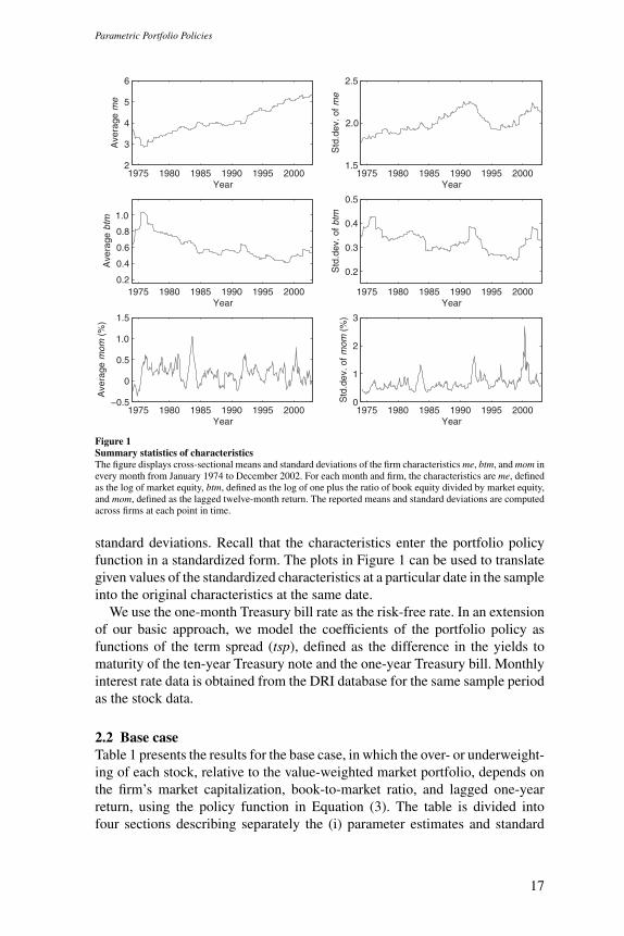
The number of firms in our sample is generally trending upward, with anaverage annual growth rate of 4.2%. The average number of firms throughoutour sample is 3680, with the fewest firms in February 1964 (1033 firms) andthe most firms in November 1997 (6356 firms).

Figure 1 describes the three firm characteristics. The first column plots thecross-sectional means of the (nonstandardized) characteristics at each monthin our sample. The second column shows the corresponding cross-sectional

12 Taking logs makes the cross-sectional distribution of me and btm more symmetric and reduces the effect ofoutliers.

16

Parametric Portfolio Policies

1975 1980 1985 1990 1995 20002

3

4

5

6

Year

Ave

rage

me

1975 1980 1985 1990 1995 20001.5

2.0

2.5

Year

Std

.dev

. of m

e

1975 1980 1985 1990 1995 20000.2

0.4

0.6

0.8

1.0

Year

Ave

rage

btm

1975 1980 1985 1990 1995 2000

0.2

0.3

0.4

0.5

Year

Std

.dev

. of b

tm

1975 1980 1985 1990 1995 2000−0.5

0

0.5

1.0

1.5

Year

Ave

rage

mom

(%

)

1975 1980 1985 1990 1995 20000

1

2

3

Year

Std

.dev

. of m

om (

%)

Figure 1Summary statistics of characteristicsThe figure displays cross-sectional means and standard deviations of the firm characteristics me, btm, and mom inevery month from January 1974 to December 2002. For each month and firm, the characteristics are me, definedas the log of market equity, btm, defined as the log of one plus the ratio of book equity divided by market equity,and mom, defined as the lagged twelve-month return. The reported means and standard deviations are computedacross firms at each point in time.

standard deviations. Recall that the characteristics enter the portfolio policyfunction in a standardized form. The plots in Figure 1 can be used to translategiven values of the standardized characteristics at a particular date in the sampleinto the original characteristics at the same date.

We use the one-month Treasury bill rate as the risk-free rate. In an extensionof our basic approach, we model the coefficients of the portfolio policy asfunctions of the term spread (tsp), defined as the difference in the yields tomaturity of the ten-year Treasury note and the one-year Treasury bill. Monthlyinterest rate data is obtained from the DRI database for the same sample periodas the stock data.

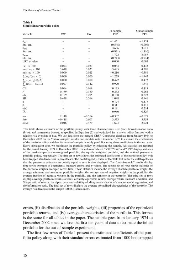
2.2 Base caseTable 1 presents the results for the base case, in which the over- or underweight-ing of each stock, relative to the value-weighted market portfolio, depends onthe firm’s market capitalization, book-to-market ratio, and lagged one-yearreturn, using the policy function in Equation (3). The table is divided intofour sections describing separately the (i) parameter estimates and standard

17

The Review of Financial Studies

Table 1Simple linear portfolio policy

In Sample Out of SampleVariable VW EW PPP PPP

θme – – −1.451 −1.124Std. err. – – (0.548) (0.709)θbtm – – 3.606 3.611Std. err. – – (0.921) (1.110)θmom – – 1.772 3.057Std. err. – – (0.743) (0.914)LRT p-value – – 0.000 0.005

|wi | × 100 0.023 0.023 0.083 0.133max wi × 100 3.678 0.023 3.485 4.391min wi × 100 0.000 0.023 −0.216 −0.386∑

wi I (wi < 0) 0.000 0.000 −1.279 −1.447∑I (wi ≤ 0)/Nt 0.000 0.000 0.472 0.472∑ |wi,t − wi,t−1| 0.097 0.142 0.990 1.341

CE 0.064 0.069 0.175 0.118r 0.139 0.180 0.262 0.262σ(r ) 0.169 0.205 0.188 0.223SR 0.438 0.564 1.048 0.941α – – 0.174 0.177β – – 0.311 0.411σ(ε) – – 0.181 0.214IR – – 0.960 0.829

me 2.118 −0.504 −0.337 −0.029btm −0.418 0.607 3.553 3.355mom 0.016 0.479 1.623 2.924

This table shows estimates of the portfolio policy with three characteristics: size (me), book-to-market ratio(btm), and momentum (mom), as specified in Equation (3) and optimized for a power utility function with arelative risk aversion of five. We use data from the merged CRSP–Compustat database from January 1964 toDecember 2002. In the “out-of-sample” results, we use data until December 1973 to estimate the coefficientsof the portfolio policy and then form out-of-sample monthly portfolios using those coefficients in the next year.Every subsequent year, we reestimate the portfolio policy by enlarging the sample. All statistics are reportedfor the period January 1974 to December 2002. The columns labeled “VW,” “EW,” and “PPP” display statisticsof the market-capitalization-weighted portfolio, the equally weighted portfolio, and the optimal parametricportfolio policy, respectively. The first set of rows shows the estimated coefficients of the portfolio policy withbootstrapped standard errors in parentheses. The bootstrapped p-value of the Wald test under the null hypothesisthat the parameter estimates are jointly equal to zero is also displayed. The “out-of-sample” results displaytime-series averages of coefficients, standard errors, and p-values. The second set of rows shows statistics ofthe portfolio weights averaged across time. These statistics include the average absolute portfolio weight, theaverage minimum and maximum portfolio weights, the average sum of negative weights in the portfolio, theaverage fraction of negative weights in the portfolio, and the turnover in the portfolio. The third set of rowsdisplays average portfolio return statistics: certainty-equivalent return, average return, standard deviation, andSharpe ratio of returns; the alpha, beta, and volatility of idiosyncratic shocks of a market model regression; andthe information ratio. The final set of rows displays the average normalized characteristics of the portfolio. Theaverage risk-free rate in the sample is 0.061 (annualized).

errors, (ii) distribution of the portfolio weights, (iii) properties of the optimizedportfolio returns, and (iv) average characteristics of the portfolio. This formatis the same for all tables in the paper. The sample goes from January 1974 toDecember 2002 since we lose the first ten years of data to estimate the initialportfolio for the out-of-sample experiments.

The first few rows of Table 1 present the estimated coefficients of the port-folio policy along with their standard errors estimated from 1000 bootstrapped

18

Parametric Portfolio Policies

samples.13 In the third column, the deviations of the optimal weights fromthe benchmark weights decrease with the firm’s market capitalization (size)and increase with both the firm’s book-to-market ratio (value) and its laggedone-year return (momentum). The signs of the estimates are consistent with theliterature. The investor overweights small firms, value firms, and past winnersand underweights large firms, growth firms, and past losers. Since the charac-teristics are standardized cross-sectionally, the magnitudes of the coefficientscan be compared to each other. Quantitatively, a high book-to-market ratioleads to the largest overweighting of a stock. All three coefficients are highlysignificant. We also test whether all three coefficients are jointly equal to zerousing a Wald test, and the bootstrapped p-value of this test is reported in therow labeled “Wald p-value.”14

The next few rows of Table 1 describe the weights of the optimized portfolio(in the second column) and compare them to the weights of the market portfolio(in the first column) and the equal-weighted portfolio (in the second column).The average absolute weight of the optimal portfolio is about four times that ofthe market (0.08% versus 0.02%). Not surprisingly, the active portfolio takeslarger positions; however, these positions are not extreme. The average (overtime) maximum and minimum weights of the optimal portfolio are 3.49%and −0.22%, respectively, while the corresponding extremes for the marketportfolio are 3.68% and 0.00%. The average sum of negative weights in theoptimal portfolio is −128%, which implies that the sum of long positions is onaverage 228%. Finally, the average fraction of negative weights (shorted stocks)in the optimal portfolio is 0.47. Overall, the optimal portfolio does not reflectunreasonably extreme bets on individual stocks and could well be implementedby a combination of an index fund that reflects the market and a long–shortequity hedge fund. Finally, one might suspect that the optimal portfolio policyrequires unreasonably large trading activity. Fortunately, this is not the case. Theaverage turnover (measured using Equation (18) as the sum of one-way trades)of the optimized portfolio is 99% per year, as compared to an average turnoverof 9.7% per year for the market portfolio (due to new listings, delistings, equityissues, etc.) and 14.2% per year for the equal-weighted portfolio. This furthershows that the optimal portfolio is eminently implementable and that the returnsare unlikely to be affected much by trading costs. Of course, the low turnoveris a result of using persistent variables. Using variables that changed morethrough time would undoubtedly result in higher turnover.

The following rows of Table 1 characterize the performance of the optimalportfolio relative to the market and the equal-weighted portfolios. For easeof interpretation, all measures are annualized. The optimal portfolio has avolatility slightly larger than that of the market portfolio but lower than the

13 We use bootstrapped standard errors since they produce slightly more conservative tests (larger standard errors)than using estimates of the asymptotic covariance matrix in Equation (12).

14 When the bootstrapped p-value from the Wald test is less than 0.001, we report it as 0.000.

19

The Review of Financial Studies

equal-weighted portfolio (18.8%, 16.9%, and 20.5%, respectively). The optimalportfolio policy has a much higher average return of 26.2% as opposed to 13.9%for the market and 18.0% for the equal-weighted portfolio. This translates intoa Sharpe ratio that is more than twice the Sharpe ratio of the market or theequal-weighted portfolio. The certainty equivalent captures the impact of theentire distribution of returns according to the risk preferences of the investorand is therefore the measure that best summarizes performance. The optimalportfolio policy offers a certainty-equivalent gain of roughly 11% relative tothe market or the equal-weighted portfolios. We can use a regression of theexcess returns of the active portfolio on the excess return of the market toevaluate the active portfolio’s alpha, market beta, and residual risk, and thenuse these statistics to compute the portfolio’s information ratio. The alpha ofthe portfolio is over 17% with a low market beta of only 0.31.15 Dividing thealpha by the residual volatility of 18.1% produces an information ratio of 0.96.Finally, a word of caution. We should point out that it is not very surprisingthat the optimal portfolio outperforms the market because we are optimizingin sample and have chosen characteristics that are known to be associated withsubstantial risk-adjusted returns.

We can decompose the optimal portfolio returns into the market return andthe return on a long–short equity hedge fund along the lines of Equation (10).The average return of this hedge fund is found to be 12.27% (not shown in thetable). We can further decompose the hedge fund return as rh = q(r+

h − r−h ),

where r+h is the return on the long part of the hedge fund and r−

h is the returnon the short part, both normalized such that the sum of their weights is one.In this way, q captures the leverage of the long–short portfolio. The averager+

h is 20.79% and the average r−h is 14.01% so that the return of the hedge

fund without leverage, i.e., with one dollar long and one dollar short positions,is 6.78%. These returns compare with the market’s return of 11.96% over thesame period. We therefore see that the long side of the hedge outperforms themarket whereas the short side has roughly the same performance as the market.In fact, the short side could be replaced with a short position in the marketportfolio without hurting performance. This is important since it is obviouslyeasier to short the market using futures than it is to hold a short portfolio ofstocks. The average return of the entire hedge fund of 12.27% and the returnsof the scaled long and short parts imply a leverage q of the long and shortpositions of the order of 173%.

To describe the composition of the optimized portfolio, we compute forevery month the weighted characteristics of the portfolio as Nt

∑Nti=1 wi,t xi,t .

The last three rows of the table compare the average (through time) weightedcharacteristics of the optimized portfolio to those of the market portfolio. The

15 The Fama–French three-factor model alpha is 9% and the four-factor alpha, including momentum, is 2.5%. Thisis consistent with our approach producing a portfolio that loads systematically on the size, value, and momentumfactor.

20

Parametric Portfolio Policies

1975 1980 1985 1990 1995 2000−2

−1

0

1

2

3

4

5

6

Year

Por

tfol

io c

hara

cter

isti

cs

mebtmmom

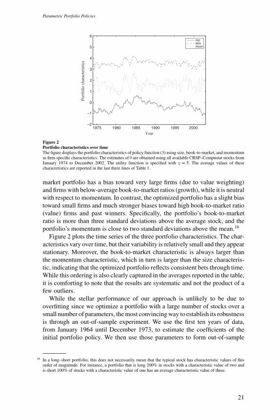
Figure 2Portfolio characteristics over timeThe figure displays the portfolio characteristics of policy function (3) using size, book-to-market, and momentumas firm-specific characteristics. The estimates of θ are obtained using all available CRSP–Compustat stocks fromJanuary 1974 to December 2002. The utility function is specified with γ = 5. The average values of thesecharacteristics are reported in the last three lines of Table 1.

market portfolio has a bias toward very large firms (due to value weighting)and firms with below-average book-to-market ratios (growth), while it is neutralwith respect to momentum. In contrast, the optimized portfolio has a slight biastoward small firms and much stronger biases toward high book-to-market ratio(value) firms and past winners. Specifically, the portfolio’s book-to-marketratio is more than three standard deviations above the average stock, and theportfolio’s momentum is close to two standard deviations above the mean.16

Figure 2 plots the time series of the three portfolio characteristics. The char-acteristics vary over time, but their variability is relatively small and they appearstationary. Moreover, the book-to-market characteristic is always larger thanthe momentum characteristic, which in turn is larger than the size characteris-tic, indicating that the optimized portfolio reflects consistent bets through time.While this ordering is also clearly captured in the averages reported in the table,it is comforting to note that the results are systematic and not the product of afew outliers.

While the stellar performance of our approach is unlikely to be due tooverfitting since we optimize a portfolio with a large number of stocks over asmall number of parameters, the most convincing way to establish its robustnessis through an out-of-sample experiment. We use the first ten years of data,from January 1964 until December 1973, to estimate the coefficients of theinitial portfolio policy. We then use those parameters to form out-of-sample

16 In a long–short portfolio, this does not necessarily mean that the typical stock has characteristic values of thisorder of magnitude. For instance, a portfolio that is long 200% in stocks with a characteristic value of two andis short 100% of stocks with a characteristic value of one has an average characteristic value of three.

21

The Review of Financial Studies

monthly portfolios during 1974. At the end of 1974 and of every subsequentyear, we reestimate the portfolio policy by enlarging the sample and applyit in every month of the following year. In this way, we estimate the policywith a “telescoping” sample and always apply it out of sample.17 The standarderrors presented are the time-series average of the standard errors from eachestimation of the optimal policy.

The out-of-sample results of our parametric portfolio policy are presented inthe last column of Table 1. The coefficients on the characteristics are roughlysimilar to the in-sample estimates, with only an increase of the importance ofmomentum. All coefficients are still statistically significant, both individuallyand jointly. The in- and out-of-sample portfolios are also remarkably similar interms of the distribution of the portfolio weights, consistent with the fact thatat least the value and momentum anomalies have been fairly stable throughoutour sample period. More importantly, there is not a large deterioration in thereturn statistics. The certainty equivalent of the portfolio policy is now 11.8%,halfway between those of the market portfolio and of the in-sample policy. Theout-of-sample comparison with the equal-weighted portfolio is of particularinterest since DeMiguel, Garlappi, and Uppal (2007) have shown that the equal-weighted portfolio generally offers a good compromise between efficiency androbustness out of sample. Our approach substantially improves the efficiencyof the portfolio without a significant loss in terms of out-of-sample robustness.We conclude from these results that our approach is likely to perform almostas well out of sample or in real time as our in-sample analysis suggests.

We showed in Equation (10) that the linear portfolio policy is similar toa static choice between long–short portfolios like those constructed by Famaand French (1993) and Carhart (1997). We construct size, book-to-market, andmomentum factors based on single sorts of all stocks based on these variables.The factor is then constructed by taking equal-weighted long positions in thestocks belonging to the top 30% and short positions in the stocks in the bottom30%. The definition of the size, book-to-market, and momentum variables usedin the sorts are the same as throughout the rest of the paper. The sample offirms is also the same. Our approach is a little different from the way Famaand French construct these factors, which relies on double sorts on size andbook-to-market. We do not follow their approach since that would be equivalentto having interaction terms in the linear policy and would make comparisonsmore difficult. Then, we simply find the weights on each of the three long–short portfolios that maximize the CRRA utility.18 Table 2 shows the results.Overall, and as expected, the results are quite similar to the results in Table 1.

17 The results are not totally out of sample to the extent that the stock characteristics used were known by us tohave significant explanatory power for the cross-section of stocks during the entire sample period. There are nosimple ways to correct this snooping bias.

18 Pastor (2000); Pastor and Stambaugh (2000); and Lynch (2001), among others, study the optimal allocation tothe Fama–French portfolios.

22

Parametric Portfolio Policies

Table 2Fama–French portfolios

In sample Out of sampleVariable VW FF FF

θme – −0.310 −0.102Std. err. – (0.211) (0.228)θbtm – 0.667 1.190Std. err. – (0.319) (0.331)θmom – 0.506 0.849Std. err. – (0.186) (0.194)LRT p-value – 0.002 0.006

|wi | × 100 0.023 0.030 0.049max wi × 100 3.678 4.596 6.694min wi × 100 0.000 −0.517 −2.167∑

wi I (wi < 0) 0.000 −0.146 −0.204∑I (wi ≤ 0)/Nt 0.000 0.403 0.388∑ |wi,t − wi,t−1| 0.097 0.328 0.484

CE 0.064 0.129 0.095r 0.139 0.216 0.240σ(r ) 0.169 0.178 0.222SR 0.438 0.847 0.805α – 0.104 0.148β – 0.627 0.524σ(ε) – 0.143 0.206IR – 0.729 0.721

me 2.118 2.311 1.935btm −0.418 −0.063 0.286mom 0.016 0.243 0.398

This table shows results for combinations of the market and three long–short portfolios constructed along thelines of Fama and French, sorted according to size, book-to-market, and momentum, optimized for a powerutility function with a relative risk aversion of five. We use data from the merged CRSP–Compustat databasefrom January 1964 to December 2002. In the “out-of-sample” results, we use data until December 1973 toestimate the coefficients of the portfolio policy and then form out-of-sample monthly portfolios using thosecoefficients in the next year. Every subsequent year, we reestimate the portfolio policy by enlarging the sample.All statistics are reported for the period January 1974 to December 2002. The columns labeled “VW” and “FF”display statistics of the market-capitalization-weighted portfolio and the optimal combination of the market withthe long–short portfolios, respectively. The first set of rows shows the estimated coefficients of the portfoliopolicy with bootstrapped standard errors in parentheses. The bootstrapped p-value of the Wald test under the nullhypothesis that the parameter estimates are jointly equal to zero is also displayed. The “out-of-sample” resultsdisplay time-series averages of coefficients, standard errors, and p-values. The second set of rows shows statisticsof the portfolio weights averaged across time. These statistics include the average absolute portfolio weight, theaverage minimum and maximum portfolio weights, the average sum of negative weights in the portfolio, theaverage fraction of negative weights in the portfolio, and the turnover in the portfolio. The third set of rowsdisplays average portfolio return statistics: certainty-equivalent return, average return, standard deviation, andSharpe ratio of returns; the alpha, beta, and volatility of idiosyncratic shocks of a market model regression; andthe information ratio. The final set of rows displays the average normalized characteristics of the portfolio. Theaverage risk-free rate in the sample is 0.061 (annualized).

The differences between the two tables are due to the fact that the Fama–French factors put a weight on each stock proportional to the firm’s marketcapitalization, whereas our linear policy puts a weight that is proportionalto the firm’s characteristic. Of course, we could easily construct long–shortportfolios like those of Fama and French where the weights are proportionalto the characteristics. In that case, using our simple linear policy would giveexactly the same results as a choice between the factor portfolios.

23

The Review of Financial Studies

Notice that the relative differences between our approach and investing inthe Fama–French portfolios carry over from the in-sample analysis to the out-of-sample results presented in the last columns of both tables. Weighting stocksby their characteristics, as opposed to equally weighting the top and bottomone-third, improves the in-sample certainty equivalent by 36% and the out-of-sample certainty equivalent by 24%.

2.3 Extensions2.3.1 Portfolio weight constraints. A large majority of equity portfoliomanagers face short-sale constraints. In Table 3, we present the results fromestimating the long-only portfolio policy specified in Equation (16), again bothin and out of sample. As in the unconstrained case, the deviation of the op-timal weight from the market portfolio weight decreases with the firm’s size,increases with its book-to-market ratio, and increases with its one-year laggedreturn. Focusing on the portfolio involving the entire universe of stocks, a highbook-to-market ratio and large positive one-year lagged return are less desirablecharacteristics for a long-only investor. The coefficients associated with bothof these characteristics are lower in magnitude than in the unrestricted caseand are only marginally significant, whereas the coefficient associated with themarket capitalization of the firm is not significant. Overall, the significance ofthe θ coefficients is substantially diminished compared to the unconstrainedbase case.

The optimal portfolio still does not involve extreme weights. In fact, theaverage maximum weight of the optimal portfolio is only 1.95%, which is ac-tually lower than that of the market portfolio. On average, the optimal portfolioinvests in only 54% of the stocks. The resulting mean and standard deviationof the portfolio return are 19.1% and 18.3%, respectively, translating into acertainly equivalent gain of 3.9% relative to holding the market portfolio. Thealpha, beta, and information ratio of the portfolio are 6.2%, 0.86, and 0.56,respectively. These statistics are quite remarkable, given the long-only con-straint. Out of sample, the certainty equivalent is 8.1%, showing some smalldeterioration relative to the in-sample optimum.

The average size of the firms in the optimal portfolio is greater than thesize of the average firm but significantly lower than that of the value-weightedmarket portfolio. The book-to-market ratio and momentum characteristics areless than one standard deviation above those of the average stock and are alsosignificantly different from those of the market portfolio. The results for theoptimal long-only portfolio in the universe of the top 500 stocks are qualitativelysimilar.

The most interesting comparison is between the long-only portfolio in Table 3and the unconstrained base case in Table 1. The difference in performance isdue to two related factors. First, the unconstrained portfolio can exploit bothpositive and negative forecasts, while the constrained portfolio can only exploitthe positive forecasts. Consistent with this argument, the fraction of short

24

Parametric Portfolio Policies

Table 3Long-only portfolio policy

In sample Out of sampleVariable VW PPP PPP

θme – −1.277 0.651Std. err. – (1.217) (1.510)θbtm – 3.215 2.679Std. err. – (1.131) (1.417)θmom – 1.416 3.780Std. err. – (1.213) (1.505)LRT p-value – 0.045 0.062

|wi | × 100 0.023 0.023 0.035max wi × 100 3.678 1.674 1.952min wi × 1000 0.000 0.000 0.000∑

wi I (wi < 0) 0.000 0.000 0.000∑I (wi ≤ 0)/Nt 0.000 0.464 0.464∑ |wi,t − wi,t−1| 0.097 0.241 0.324

CE 0.064 0.103 0.081r 0.139 0.191 0.177σ(r ) 0.169 0.183 0.187SR 0.438 0.690 0.618α – 0.062 0.057β – 0.862 0.943σ(ε) – 0.111 0.094IR – 0.561 0.601

me 2.118 0.070 0.634btm −0.418 0.985 0.345mom 0.016 0.396 1.106

This table shows estimates of the portfolio policy with long-only weights in Equation (16) with three character-istics: size (me), book-to-market ratio (btm), and momentum (mom), optimized for a power utility function witha relative risk aversion of five. We use data from the merged CRSP–Compustat database from January 1964 toDecember 2002. In the “out-of-sample” results, we use data until December 1973 to estimate the coefficientsof the portfolio policy and then form out-of-sample monthly portfolios using those coefficients in the next year.Every subsequent year, we reestimate the portfolio policy by enlarging the sample. All statistics are reportedfor the period January 1974 to December 2002. The columns labeled “VW” and “PPP” display statistics of themarket-capitalization-weighted portfolio and the optimal parametric portfolio policy, respectively. The first setof rows shows the estimated coefficients of the portfolio policy with bootstrapped standard errors in parentheses.The bootstrapped p-value of the Wald test under the null hypothesis that the parameter estimates are jointlyequal to zero is also displayed. The “out-of-sample” results display time-series averages of coefficients, standarderrors, and p-values. The second set of rows shows statistics of the portfolio weights, averaged across time.These statistics include the average absolute portfolio weight, the average minimum and maximum portfolioweights, the average sum of negative weights in the portfolio, the average fraction of negative weights in theportfolio, and the turnover in the portfolio. The third set of rows displays average portfolio return statistics:certainty-equivalent return, average return, standard deviation, and Sharpe ratio of returns; the alpha, beta, andvolatility of idiosyncratic shocks of a market model regression; and the information ratio. The final set of rowsdisplays the average normalized characteristics of the portfolio. The average risk-free rate in the sample is 0.061(annualized).

positions in Table 1 is roughly the same as the fraction of stocks not heldby the long portfolio in Table 3. Second, the unconstrained portfolio benefitsfrom using the short positions as leverage to increase the exposure to the longpositions.

Interestingly, the tests for joint significance of all three parameters have ap-value around 5%. We therefore cannot reject that the coefficients are jointlyzero and that the investor is equally well off holding the market as holdingthe optimal portfolio. This rejection is consistent with the increase in the

25

The Review of Financial Studies

standard errors on the coefficients and the smaller gain in certainty equivalentof the restricted optimal portfolio relative to the market. We conclude thatshort sales constraints have some power in explaining the size, value, andmomentum anomalies. An interesting consequence is that market frictions thathave constrained investors’ ability to short sell stocks (that were more prevalentin the past but that still have an impact) may have limited the arbitraging of theanomalies.

2.3.2 Time-varying coefficients. In Table 4, we allow the coefficients of theportfolio policy to depend on the slope of the yield curve. We estimate differentcoefficients for months when the yield curve at the beginning of the monthis positively sloped (normal) and negatively sloped (inverted). Since invertedyield curves tend to be associated with recessions, letting the portfolio coef-ficients vary with the yield-curve slope allows the effect of the characteristicson the joint distribution of returns to be different during expansionary andcontractionary periods.

We present both in- and out-of-sample results in Table 4. In both cases,the most dramatic effect of conditioning on the slope of the yield curve is onthe role of the size of the firm. When the yield curve is upward sloping, theoptimal portfolio is tilted toward smaller firms, just as in the base case. Whenthe yield curve is downward sloping, in contrast, the tilt is exactly the opposite,with a positive coefficient (although not statistically different from zero). Thisis consistent with the common notion that small firms are more affected byeconomic downturns than larger and more diversified firms. For book-to-marketand momentum, the coefficients are generally larger in magnitude when theyield curve slopes down.

Conditioning on the slope of the yield curve does not significantly alterthe distribution of the optimal portfolio weights; however, the performanceof the portfolio is improved. Both in and out of sample, the portfolios havehigher average returns, certainly equivalents, alphas, and information ratios,than without conditioning.

The average characteristics of the optimal portfolios are the most interestingto analyze. Consider the in-sample case. As suggested by the coefficient esti-mates, the optimal portfolio is tilted toward small stocks when the yield curveis upward sloping. When the yield curve is downward sloping, the portfolio istilted toward larger stocks and resembles closely the composition of the marketportfolio. The average book-to-market and momentum characteristics are bothpositive and larger when the yield slope is positive. It is interesting to notethat although the theta coefficient on book-to-market with an inverted yieldcurve is very different from the corresponding coefficient in sample, there is nocorresponding change in the average characteristic of the portfolio. Intuitively,this arises from the joint distribution of the characteristics conditional on theslope of the yield curve.

26

Parametric Portfolio Policies

Table 4Conditioning on the slope of the yield curve

In sample Out of sampleVariable VW PPP PPP

θme×I (tsp>0) – −2.168 −1.844Std. err. – (0.706) (0.745)θme×I (tsp≤0) – 1.684 3.186Std. err. – (1.196) (1.207)θbtm×I (tsp>0) – 3.197 3.146Std. err. – (1.102) (1.121)θbtm×I (tsp≤0) – 5.830 0.037Std. err. – (2.061) (0.879)θmom×I (tsp>0) – 2.023 4.489Std. err. – (0.909) (1.597)θmom×I (tsp≤0) – 3.705 3.598Std. err. – (1.611) (1.108)LRT p-value – 0.000 0.000

|wi | × 100 0.023 0.091 0.136max wi × 100 3.678 3.489 4.392min wi × 1000 0.000 −2.619 −0.398∑

wi I (wi < 0) 0.000 −1.428 −1.526∑I (wi ≤ 0)/Nt 0.000 0.476 0.476∑ |wi,t − wi,t−1| 0.097 1.295 1.510

CE 0.064 0.194 0.120r 0.139 0.293 0.277σ(r ) 0.169 0.205 0.236SR 0.438 1.114 0.932α – 0.209 0.197β – 0.252 0.319σ(ε) – 0.201 0.231IR – 1.042 0.851

me × I(tsp > 0) 1.748 −0.744 −0.430me × I(tsp ≤ 0) 0.370 0.351 0.129btm I(tsp > 0) −0.342 2.782 2.544btm × I(tsp ≤ 0) −0.076 0.789 0.880mom I(tsp > 0) 0.031 1.583 2.381mom × I(tsp ≤ 0) −0.015 0.529 0.740

This table shows estimates of the portfolio policy with the product of three characteristics: size (me), book-to-market ratio (btm), and momentum (mom), and an indicator function of the sign of the slope of the yieldcurve, optimized for a power utility function with a relative risk aversion of five. We use data from the mergedCRSP–Compustat database from January 1964 to December 2002. In the “out-of-sample” results, we use datauntil December 1973 to estimate the coefficients of the portfolio policy and then form out-of-sample monthlyportfolios using those coefficients in the next year. Every subsequent year, we reestimate the portfolio policy byenlarging the sample. All statistics are reported for the period January 1974 to December 2002. The columnslabeled “VW” and “PPP” display statistics of the market-capitalization-weighted portfolio and the optimalparametric portfolio policy, respectively. The first set of rows shows the estimated coefficients of the portfoliopolicy with bootstrapped standard errors in parentheses. The bootstrapped p-value of the Wald test under the nullhypothesis that the parameter estimates are jointly equal to zero is also displayed. The “out-of-sample” resultsdisplay time-series averages of coefficients, standard errors, and p-values. The second set of rows shows statisticsof the portfolio weights averaged across time. These statistics include the average absolute portfolio weight, theaverage minimum and maximum portfolio weights, the average sum of negative weights in the portfolio, theaverage fraction of negative weights in the portfolio, and the turnover in the portfolio. The third set of rowsdisplays average portfolio return statistics: certainty-equivalent return, average return, standard deviation, andSharpe ratio of returns; the alpha, beta, and volatility of idiosyncratic shocks of a market model regression; andthe information ratio. The final set of rows displays the average normalized characteristics of the portfolio. Theaverage risk-free rate in the sample is 0.061 (annualized).

27

The Review of Financial Studies

Table 5Varying risk aversion

In sample Out of samplePPP PPP

Variable VW γ = 1 γ = 5 γ = 100 γ = 1 γ = 5 γ = 100

θme – −6.242 −1.124 0.026 −7.178 0.651 0.824Std. err. – (2.882) (0.548) (0.223) (4.579) (0.709) (0.212)θbtm – 7.864 3.611 5.207 8.450 2.679 3.834Std. err. – (3.546) (0.921) (0.314) (3.435) (1.110) (0.346)θmom – 6.452 3.057 0.548 11.991 3.780 −0.105Std. err. – (2.915) (0.743) (0.483) (2.971) (0.914) (0.205)LRT p-value – 0.000 0.000 0.000 0.000 0.000 0.000

|wi | × 100 0.023 0.217 0.133 0.102 0.422 0.035 0.114max wi × 100 3.678 3.623 4.391 3.585 6.106 1.952 4.621min wi × 100 0.000 −0.646 −0.386 −0.238 −1.309 0.000 −0.327∑

wi I (wi < 0) 0.000 −4.122 −1.447 −1.670 −5.582 0.000 −1.201∑I (wi ≤ 0)/Nt 0.000 0.522 0.472 0.477 0.529 0.464 0.460∑ |wi,t − wi,t−1| 0.097 3.010 1.341 0.883 4.797 0.324 0.608

CE 0.064 0.360 0.118 −0.989 0.297 0.081 −1.408r 0.139 0.534 0.262 0.223 0.673 0.177 0.147σ(r ) 0.169 0.589 0.223 0.199 0.847 0.187 0.170SR 0.438 0.796 0.941 0.796 0.726 0.618 0.557α – 0.529 0.177 0.141 0.647 0.057 0.058β – −0.817 0.411 0.229 −0.602 0.943 0.465σ(ε) – 0.573 0.214 0.195 0.842 0.094 0.153IR – 0.924 0.829 0.723 0.768 0.601 0.380

me 2.118 −6.234 −0.029 0.633 −7.328 0.634 1.763btm −0.418 9.060 3.355 4.761 9.633 0.345 3.105mom 0.016 6.016 2.924 0.391 11.621 1.106 −0.233

This table shows estimates of the linear portfolio policy (3) with three characteristics: size (me), book-to-marketratio (btm), and momentum (mom) optimized for different power utility functions with a relative risk aversionof one, five (as in previous tables), and 100. We use data from the merged CRSP–Compustat database fromJanuary 1964 to December 2002. In the “out-of-sample” results, we use data until December 1973 to estimatethe coefficients of the portfolio policy and then form out-of-sample monthly portfolios using those coefficients inthe next year. Every subsequent year, we reestimate the portfolio policy by enlarging the sample. All statistics arereported for the period January 1974 to December 2002. The columns labeled “VW” and “PPP” display statisticsof the market-capitalization-weighted portfolio and the optimal parametric portfolio policy, respectively. Thefirst set of rows shows the estimated coefficients of the portfolio policy with bootstrapped standard errors inparentheses. The bootstrapped p-value of the Wald test under the null hypothesis that the parameter estimates arejointly equal to zero is also displayed. The “out-of-sample” results display time-series averages of coefficients,standard errors, and p-values. The second set of rows shows statistics of the portfolio weights averaged acrosstime. These statistics include the average absolute portfolio weight, the average minimum and maximum portfolioweights, the average sum of negative weights in the portfolio, the average fraction of negative weights in theportfolio, and the turnover in the portfolio. The third set of rows displays average portfolio return statistics:certainty-equivalent return, average return, standard deviation, and Sharpe ratio of returns; the alpha, beta, andvolatility of idiosyncratic shocks of a market model regression; and the information ratio. The final set of rowsdisplays the average normalized characteristics of the portfolio. The average risk-free rate in the sample is 0.061(annualized). The certainty-equivalent returns of the market portfolio for γ = 1, γ = 5, and γ = 100 are 0.107,0.052, and −1.976 (annualized), respectively.

2.3.3 Risk aversion. The optimal portfolio policy depends critically on theinvestor’s preferences. The results thus far were obtained assuming CRRAutility with relative risk aversion γ = 5. To get a better sense for the role ofthis utility assumption, we present in Table 5 in- and out-of-sample resultsfor different levels of risk aversion. In addition to γ = 5, which we reportin the table for comparison, we also estimate the optimal portfolio for γ = 1,

28

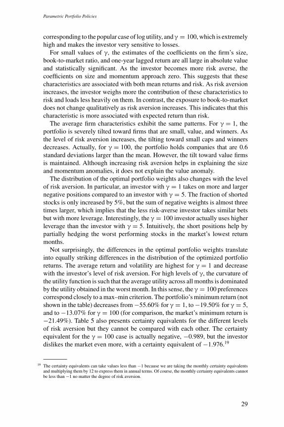
Parametric Portfolio Policies

corresponding to the popular case of log utility, and γ = 100, which is extremelyhigh and makes the investor very sensitive to losses.

For small values of γ, the estimates of the coefficients on the firm’s size,book-to-market ratio, and one-year lagged return are all large in absolute valueand statistically significant. As the investor becomes more risk averse, thecoefficients on size and momentum approach zero. This suggests that thesecharacteristics are associated with both mean returns and risk. As risk aversionincreases, the investor weighs more the contribution of these characteristics torisk and loads less heavily on them. In contrast, the exposure to book-to-marketdoes not change qualitatively as risk aversion increases. This indicates that thischaracteristic is more associated with expected return than risk.

The average firm characteristics exhibit the same patterns. For γ = 1, theportfolio is severely tilted toward firms that are small, value, and winners. Asthe level of risk aversion increases, the tilting toward small caps and winnersdecreases. Actually, for γ = 100, the portfolio holds companies that are 0.6standard deviations larger than the mean. However, the tilt toward value firmsis maintained. Although increasing risk aversion helps in explaining the sizeand momentum anomalies, it does not explain the value anomaly.

The distribution of the optimal portfolio weights also changes with the levelof risk aversion. In particular, an investor with γ = 1 takes on more and largernegative positions compared to an investor with γ = 5. The fraction of shortedstocks is only increased by 5%, but the sum of negative weights is almost threetimes larger, which implies that the less risk-averse investor takes similar betsbut with more leverage. Interestingly, the γ = 100 investor actually uses higherleverage than the investor with γ = 5. Intuitively, the short positions help bypartially hedging the worst performing stocks in the market’s lowest returnmonths.

Not surprisingly, the differences in the optimal portfolio weights translateinto equally striking differences in the distribution of the optimized portfolioreturns. The average return and volatility are highest for γ = 1 and decreasewith the investor’s level of risk aversion. For high levels of γ, the curvature ofthe utility function is such that the average utility across all months is dominatedby the utility obtained in the worst month. In this sense, the γ = 100 preferencescorrespond closely to a max–min criterion. The portfolio’s minimum return (notshown in the table) decreases from −55.60% for γ = 1, to −19.50% for γ = 5,and to −13.07% for γ = 100 (for comparison, the market’s minimum return is−21.49%). Table 5 also presents certainty equivalents for the different levelsof risk aversion but they cannot be compared with each other. The certaintyequivalent for the γ = 100 case is actually negative, −0.989, but the investordislikes the market even more, with a certainty equivalent of −1.976.19

19 The certainty equivalents can take values less than −1 because we are taking the monthly certainty equivalentsand multiplying them by 12 to express them in annual terms. Of course, the monthly certainty equivalents cannotbe less than −1 no matter the degree of risk aversion.

29

The Review of Financial Studies

Comparing the in- and out-of-sample results, it appears that our methodperforms better out of sample for lower levels of risk aversion than for higherlevels of risk aversion. This can be seen equivalently from the differences in thepolicy coefficients, in the performance measures, or in the portfolio character-istics. For example, with γ = 1, the in-sample average portfolio characteristicsare me = −6.234, btm = 9.060, and mom = 6.016; the corresponding out-of-sample average portfolio characteristics are −7.328, 9.633, and 11.621.In contrast, with γ = 100, the relative differences between the in- and out-of-sample characteristics are much greater: me of 0.633 versus 1.763, btm of 4.761versus 3.105, and mom of 0.391 versus −0.233. Apparently, risk-minimizingportfolios are less stable than expected return-maximizing portfolios.

2.4 Transaction costsIn this section, we examine the impact of transaction costs on optimal tradingpolicies. As a first approach, we take one-way transaction costs to be constantthrough time and in the cross-section at 0.5%. However, it is well known thattransaction costs vary considerably across stocks, being larger for small capsthan for large caps, and have been gradually decreasing over time. This has beennoted by Keim and Madhavan (1997); Domowitz, Glen, and Madhavan (2001);and Hasbrouck (2006). To accommodate these empirical facts, we use a secondspecification for transaction costs, which allows for cross-sectional variationand captures the declining costs over time. The one-way cost of company i attime t is ci,t = zi,t ∗ Tt . The variable zi,t = 0.006 − 0.0025 × mei,t capturesthe cross-sectional variation in transaction costs with the market cap of thefirms. In this specification, mei,t measures the relative size of company i attime t , normalized to be between 0 and 1. In other words, the smallest companyhas a transaction cost of 0.6%, whereas the largest one has a cost of 0.35%.This is consistent with previous estimates (e.g., Keim and Madhavan 1997 andHasbrouck 2006). We capture the declining transaction costs over the sampleby assuming a trend Tt such that costs in 1974 are four times larger than those in2002. This again is consistent with the Domowitz, Glen, and Madhavan (2001)and Hasbrouck (2006) papers. The average ci,t at the end of the sample is 0.5%,which is directly comparable to the constant cost case. Figure 3 displays themedian, minimum, and maximum trading costs over time.

Table 6 presents the results for the simple linear policy (3) optimized withthe two transaction cost scenarios described above. For comparison, we alsoinclude the case with no transaction costs from Table 1. We see that transactioncosts lead to a slight decrease in the absolute value of the optimal thetas,reflecting the overall higher cost of trading. Note that in the limit with zerothetas, the policy would be equal to the market portfolio and there wouldbe substantially less trading. Indeed, we see that turnover goes down with theincreasing levels of trading costs. The effect is not very pronounced becausethe variables we are using in the portfolio policy are very persistent and inducerelatively low levels of turnover compared to the high expected returns they

30

Parametric Portfolio Policies

1975 1980 1985 1990 1995 2000

0.005

0.015

0.025

0.035

Year

One

-way

tran

sact

ion

cost

s

Figure 3Varying transaction costsThe figure displays the transaction costs described in Section 1.4. The transaction costs are assumed to declineuniformly over time and to decrease with the relative size of the firms. The solid line is the median transactioncost across all stocks over time. The dashed lines are the minimum and maximum transaction costs over time.

generate. With a turnover of 100% per year, average costs of 0.5% generate atrading cost of only 0.5%.

Table 7 shows the results obtained by applying the policy with a no-tradeboundary developed in Section 1.4. This policy leads to roughly 30% lessturnover than the simple linear policy with a substantial increase in certaintyequivalent. This is especially remarkable out of sample, where there is virtuallyno loss in performance. Intuitively, this is due to the smoothing features of theautoregressive policy. By making weights less volatile through time, this policyessentially becomes more robust out of sample. Note that the weight put onthe portfolio from the previous month (αt ) is on average slightly above 50%,reflecting the substantial inertia in the optimal portfolio policy.

Comparing the in-sample results in the first few columns of Tables 6 and 7to their respective out-of-sample counterparts in the last three columns of eachtable, we observe that the effect of incorporating transaction costs is roughlyequivalent in and out of sample. The underlying reason is that the in- and out-of-sample policies are very similar in the base case. Therefore, the turnover isvery similar in the base case, and the effect of incorporating this turnover andthe resulting transaction costs are also very similar.

3. Conclusion

We proposed a novel approach to optimizing large-scale equity portfolios.The portfolio weight in each stock is modeled as a function of the firm’scharacteristics, such as its market capitalization, book-to-market ratio, andlagged return. The coefficients of this function are found by optimizing theinvestor’s average utility of the portfolio’s return over a given sample period.

31

The Review of Financial Studies

Table 6Simple portfolio policy with transactions costs

In-sample PPP Out-of-sample PPPci,t = ci,t =

Variable VW 0.000 0.005 f (mei,t , t) 0.000 0.005 f (mei,t , t)

θme – −1.451 −1.391 −1.167 −1.124 −1.105 −0.925Std. err. – (0.548) (0.547) (0.550) (0.709) (0.849) (0.780)θbtm – 3.606 3.557 3.160 3.611 3.618 3.468Std. err. – (0.921) (0.922) (0.924) (1.110) (1.125) (1.305)θmom – 1.772 1.651 1.307 3.057 3.028 2.497Std. err. – (0.743) (0.741) (0.745) (0.914) (0.952) (0.961)LRT p-value – 0.000 0.000 0.000 0.005 0.006 0.008

|wi | × 100 0.023 0.083 0.082 0.074 0.133 0.133 0.084max wi × 100 3.678 3.485 3.491 3.508 4.391 4.392 3.535min wi × 100 0.000 −0.216 −0.208 −0.183 −0.386 −0.385 −0.233∑

wi I (wi < 0) 0.000 −1.279 −1.240 −1.074 −1.447 −1.444 −1.301∑I (wi ≤ 0)/Nt 0.000 0.472 0.471 0.463 0.472 0.472 0.464∑ |wi − wh

i | 0.097 0.990 0.942 0.788 1.341 1.333 1.087

CE|ci,t = 0.000 0.064 0.175 0.175 0.173 0.118 0.123 0.122CE|ci,t = 0.005 – 0.169 0.170 0.168 0.115 0.117 0.118CE|ci,t = f (mei,t , t) – 0.162 0.162 0.167 0.119 0.120 0.125r 0.139 0.262 0.252 0.243 0.262 0.248 0.244σ(r ) 0.169 0.188 0.183 0.179 0.223 0.220 0.217SR 0.438 1.048 1.021 0.978 0.941 0.889 0.880α – 0.174 0.162 0.151 0.177 0.163 0.152β – 0.311 0.328 0.354 0.411 0.416 0.421σ(ε) – 0.181 0.175 0.171 0.214 0.210 0.206IR – 0.960 0.929 0.887 0.829 0.774 0.764

me 2.118 −0.337 −0.267 −0.033 −0.029 −0.018 0.252btm −0.418 3.553 3.492 3.066 3.355 3.362 3.237mom 0.016 1.623 1.477 1.279 2.924 2.896 2.369

This table shows estimates of the portfolio policy with three characteristics: size (me), book-to-market ratio(btm), and momentum (mom), as specified in Equation (3) and optimized for a power utility function with arelative risk aversion of five. The utility function is maximized for returns after transaction costs. In the firstspecification, the proportional transaction costs are 0.5%, constant across stocks and over time. In the secondspecification, transaction costs vary across stocks and over time as shown in Figure 3. For comparison, wealso present results with zero transaction costs. We use data from the merged CRSP–Compustat database fromJanuary 1964 to December 2002. In the “out-of-sample” results, we use data until December 1973 to estimatethe coefficients of the portfolio policy and then form out-of-sample monthly portfolios using those coefficientsin the next year. Every subsequent year, we reestimate the portfolio policy by enlarging the sample. All statisticsare reported for the period January 1974 to December 2002. The first set of rows shows the estimated coefficientsof the portfolio policy with bootstrapped standard errors in parentheses. The bootstrapped p-value of the Waldtest under the null hypothesis that the parameter estimates are jointly equal to zero is also displayed. The “out-of-sample” results display time-series averages of coefficients, standard errors, and p-values. The second set ofrows shows statistics of the portfolio weights, averaged across time. These statistics include the average absoluteportfolio weight, the average minimum and maximum portfolio weights, the average sum of negative weightsin the portfolio, the average fraction of negative weights in the portfolio, and the turnover in the portfolio. Thethird set of rows displays average portfolio return statistics: certainty-equivalent returns, average return, standarddeviation, and Sharpe ratio of returns; the alpha, beta, and volatility of idiosyncratic shocks of a market modelregression; and the information ratio. We compute the certainty-equivalent return for the policy with and withoutadjustment for transaction costs. The final set of rows displays the average normalized characteristics of theportfolio. The average risk-free rate in the sample is 0.061 (annualized).

We argued that our approach is computationally simple, easily modified andextended, produces sensible portfolio weights, and offers robust performancein and out of sample.

We illustrated many features of our approach through an empirical applica-tion to the universe of stocks in the CRSP–Compustat data set. Our empirical

32

Parametric Portfolio Policies

Table 7Boundary portfolio policy with transactions costs

In-sample PPP Out-of-sample PPPci,t = ci,t =

Variable VW 0.000 0.005 f (mei,t , t) 0.000 0.005 f (mei,t , t)

θme – −1.147 −1.133 −0.947 −0.979 −0.946 −0.845Std. err. – (0.561) (0.537) (0.523) (0.577) (0.571) (0.568)θbtm – 4.432 4.405 4.194 4.264 4.150 4.021Std. err. – (1.137) (1.124) (1.077) (1.153) (1.232) (1.247)θmom – 2.366 2.344 2.205 3.587 3.498 3.154Std. err. – (0.964) (0.846) (0.824) (1.007) (0.943) (0.948)κ × 103 – 0.273 0.282 0.301 0.289 0.294 0.307Std. err. – (0.078) (0.087) (0.091) (0.084) (0.094) (0.098)LRT p-value – 0.000 0.000 0.000 0.000 0.000 0.000|wi | × 100 0.023 0.095 0.094 0.089 0.100 0.098 0.097max wi × 100 3.678 3.481 3.481 3.495 3.503 3.505 3.504min wi × 100 0.000 −0.362 −0.363 −0.356 −0.401 −0.395 −0.398∑

wi I (wi < 0) 0.000 −1.516 −1.499 −1.388 −1.636 −1.581 −1.566∑I (wi ≤ 0)/Nt 0.000 0.478 0.477 0.474 0.476 0.474 0.474∑ |wi − wh

i | 0.098 0.697 0.676 0.591 0.934 0.888 0.795

CE|ci,t = 0.000 0.064 0.187 0.187 0.187 0.169 0.172 0.176CE|ci,t = 0.005 – 0.183 0.184 0.183 0.158 0.161 0.159CE|ci,t = f (mei,t , t) – 0.177 0.178 0.181 0.160 0.164 0.167r 0.139 0.280 0.275 0.266 0.293 0.289 0.284σ(r ) 0.169 0.195 0.193 0.189 0.223 0.217 0.212SR 0.438 1.105 1.088 1.065 1.021 1.028 1.032α – 0.196 0.190 0.180 0.208 0.202 0.198β – 0.266 0.275 0.292 0.272 0.295 0.299σ(ε) – 0.190 0.188 0.183 0.219 0.212 0.206IR – 1.028 1.010 0.982 0.950 0.952 0.961

me 2.118 −0.189 −0.164 0.085 0.057 0.123 0.257btm −0.418 4.015 3.970 3.670 3.777 3.648 3.469mom 0.016 1.959 1.927 1.768 3.098 3.002 2.645

avg α – 0.556 0.572 0.620 0.497 0.514 0.563min α – 0.260 0.269 0.300 0.247 0.267 0.294max α – 0.828 0.842 0.882 0.740 0.758 0.811

This table shows estimates of the portfolio policy with three characteristics: size (me), book-to-market ratio(btm), and momentum (mom), as specified in Section 1.4 and optimized for a power utility function with arelative risk aversion of five. The utility function is maximized for returns after transaction costs. In the firstspecification, the proportional transaction costs are 0.5%, constant across stocks and over time. In the secondspecification, transaction costs vary across stocks and over time as shown in Figure 3. For comparison, wealso present results with zero transaction costs. We use data from the merged CRSP–Compustat database fromJanuary 1964 to December 2002. In the “out-of-sample” results, we use data until December 1973 to estimatethe coefficients of the portfolio policy and then form out-of-sample monthly portfolios using those coefficientsin the next year. Every subsequent year, we reestimate the portfolio policy by enlarging the sample. All statisticsare reported for the period January 1974 to December 2002. The first set of rows shows the estimated coefficientsof the portfolio policy with bootstrapped standard errors in parentheses. The bootstrapped p-value of the Waldtest under the null hypothesis that the parameter estimates are jointly equal to zero is also displayed. The “out-of-sample” results display time-series averages of coefficients, standard errors, and p-values. The second set ofrows shows statistics of the portfolio weights averaged across time. These statistics include the average absoluteportfolio weight, the average minimum and maximum portfolio weights, the average sum of negative weightsin the portfolio, the average fraction of negative weights in the portfolio, and the turnover in the portfolio. Thethird set of rows displays average portfolio return statistics: certainty-equivalent returns, average return, standarddeviation, and Sharpe ratio of returns; the alpha, beta, and volatility of idiosyncratic shocks of a market modelregression; and the information ratio. We compute the certainty-equivalent return for the policy with and withoutadjustment for transaction costs. The final set of rows displays the average normalized characteristics of theportfolio. The average risk-free rate in the sample is 0.061 (annualized).

33

The Review of Financial Studies

results document the importance of the firm’s market capitalization, book-to-market ratio, and one-year lagged return for explaining deviations of the optimalportfolio for a CRRA investor from the market. Relative to market capitaliza-tion weights, the optimal portfolio (with and without short-sale constraints)allocates considerably more wealth to stocks of small firms, firms with highbook-to-market ratios (value firms), and firms with large positive lagged returns(past winners). With a relative risk aversion of five, the certainty-equivalent gainfrom incorporating the firm characteristics, relative to holding the market port-folio, is an annualized 11%. We showed that these results are robust out ofsample. Finally, we incorporated transaction costs. We showed that, with asimple policy function that features a no-trade boundary, the portfolio turnoveris reduced by up to 50% with only marginal deterioration in performance.

Our idea can easily be applied to other asset classes. We could use a similarapproach to form bond portfolios based on bond characteristics (e.g., duration,convexity, coupon rate, credit rating, leverage) or to form currency portfoliosbased on the characteristics of each country pair (e.g., interest rate and inflationrate differentials, trade balance).

Appendix: Data

For each firm in the CRSP–Compustat data set, we construct several variables at the end of fiscalyears 1964 to 2002. The first full year of data, 1963, is used to construct lagged values. Theexact fiscal year-end dates are from CRSP. We use the following quantities in the definition ofthe variables (Compustat data item numbers are in parentheses): total assets (6); liabilities (181);preferred stock value (10, 56, or 130, in that order, otherwise zero); balance sheet deferred taxes andinvestment tax credits (35, otherwise zero); price per share (from CRSP); and shares outstanding(25, otherwise taken from CRSP). If total assets, liabilities, price, and shares outstanding aremissing, the observation is not included in the data set. Then, we define book equity (BE) as equalto total assets minus liabilities plus balance sheet deferred taxes and investment tax credits minuspreferred stock value; market equity (ME) as equal to price per share times shares outstanding;book-to-market (btm) as equal to the log of one plus book equity divided by market equity. Weomit firms with negative book-to-market ratio. Log market equity (me) is computed as the log ofmarket equity.

The monthly firm returns are obtained from CRSP. We allow a minimum of a six-month lagbetween the fiscal year end of the above accounting variables and the returns to ensure that theinformation from the firms’ annual reports would have been publicly available at the time ofportfolio formation. From CRSP, we also compute the trailing twelve-month return (mom) definedas the monthly compounded return between months t − 13 and t − 2. After all variables have beencreated, we eliminate the smallest 20% of firms (i.e., firms in the lowest 20th percentile of me).

ReferencesAıt-Sahalia, Y., and M. W. Brandt. 2001. Variable Selection for Portfolio Choice. Journal of Finance 56:1297–351.

Akian, M., J. Luis Menaldi, and A. Sulem. 1996. On an Investment-Consumption Model with Transactions Costs.SIAM Journal of Control and Optimization 34:329–64.

Alexander, G., and A. Baptista. 2002. Economic Implications of Using a Mean–VaR Model for PortfolioSelection: A Comparison with Mean–Variance Analysis. Journal of Economic Dynamics and Control 26:1159–93.

34

Parametric Portfolio Policies

Ang, A., G. Bekaert, and J. Liu. 2005. Why Stocks May Disappoint. Journal of Financial Economics 76:471–508.

Asness, C. S., B. Porter, and R. L. Stevens. 2001. Predicting Stock Returns Using Industry-Relative FirmCharacteristics. Working Paper, AQR Capital Management.

Basak, S., and A. Shapiro. 2001. Value-at-Risk Based Risk Management: Optimal Policies and Asset Prices.Review of Financial Studies 14:371–405.

Benartzi, S., and R. H. Thaler. 1995. Myopic Loss Aversion and the Equity Premium Puzzle. Quarterly Journalof Economics 110:73–92.

Black, F., and R. Litterman. 1992. Global Portfolio Optimization. Financial Analysts Journal 48:28–43.

Brandt, M. W. 1999. Estimating Portfolio and Consumption Choice: A Conditional Method of Moments Ap-proach. Journal of Finance 54:1609–46.

Brandt, M. W. Forthcoming. Portfolio Choice Problems. In Y. Aıt-Sahalia and L.P. Hansen (eds.), Handbook ofFinancial Econometrics.

Brandt, M. W., and P. Santa-Clara. 2006. Dynamic Portfolio Selection by Augmenting the Asset Space. Journalof Finance 61:2187–217.

Browne, S. 1999. Beating a Moving Target: Optimal Portfolio Strategies for Outperforming a Stochastic Bench-mark. Finance and Stochastics 3:275–94.

Campbell, J. Y. 1991. A Variance Decomposition for Stock Returns. Economic Journal 101:157–79.

Campbell, J. Y., and R. J. Shiller. 1988. Stock Prices, Earnings, and Expected Dividends. Journal of Finance43:661–76.

Carhart, M. M. 1997. On Persistence in Mutual Fund Performance. Journal of Finance 52:57–82.

Chan, K. C., J. Karceski, and J. Lakonishok. 1998. The Risk and Return from Factors. Journal of Financial andQuantitative Analysis 33:159–88.

Chan, K. C., J. Karceski, and J. Lakonishok. 1999. On Portfolio Optimization: Forecasting Covariances andChoosing the Risk Model. Review of Financial Studies 12:937–74.

Cooper, M., H. Gulen, and M. Vassalou. 2000. Investing in Size and Book-to-Market Portfolios Using InformationAbout the Macroeconomy: Some New Trading Rules. Working Paper, Purdue University.

Daniel, K. D., and S. Titman. 1999. Market Efficiency in an Irrational World. Financial Analyst Journal 55:24–50.

Davis, M. H. A., and A. R. Norman. 1990. Portfolio Selection with Transaction Costs. Mathematics of OperationsResearch 15:676–713.

DeMiguel, V., L. Garlappi, and R. Uppal. Forthcoming. Optimal Versus Naive Diversification: How Inefficientis the 1/N Portfolio Strategy? Review of Financial Studies.

Dixit, A. 1991. A Simplified Treatment of Some Results Concerning Regulated Brownian Motion. Journal ofEconomic Dynamics and Control 15:657–74.

Domowitz, I., J. Glen, and A. Madhavan. 2001. Liquidity, Volatility, and Equity Trading Costs Across Countriesand Over Time. International Finance 4:221–55.

Dumas, B. 1991. Super Contact and Related Optimality Conditions. Journal of Economic Dynamics and Control15:675–86.

Fama, E. F. 1990. Stock Returns, Expected Returns, and Real Activity. Journal of Finance 45:1089–108.

Fama, E. F., and K. R. French. 1988. Permanent and Temporary Components of Stock Prices. Journal of PoliticalEconomy 96:246–73.

Fama, E. F., and K. R. French. 1989. Business Conditions and Expected Returns on Stocks and Bonds. Journalof Financial Economics 25:23–49.

35

The Review of Financial Studies

Fama, E. F., and K. R. French. 1993. Common Risk Factors in the Returns of Stocks and Bonds. Journal ofFinancial Economics 33:3–56.

Fama, E. F., and K. R. French. 1996. Multifactor Explanations of Asset Pricing Anomalies. Journal of Finance51:55–84.

Frost, P. A., and J. E. Savarino. 1986. An Empirical Bayes Approach to Efficient Portfolio Selection. Journal ofFinancial and Quantitative Analysis 21:293–305.

Frost, P. A., and J. E. Savarino. 1988. For Better Performance: Constrain Portfolio Weights. Journal of PortfolioManagement 15:29–34.

Gomes, F. 2005. Portfolio Choice and Trading Volume with Loss-Averse Investors. Journal of Business 78:675–706.

Grossman, S. J., and J. Vila. 1989. Portfolio Insurance in Complete Markets: A Note. Journal of Business62:473–76.

Hansen, L. P. 1982. Large Sample Properties of Generalized Method of Moments Estimators. Econometrica50:1029–53.

Hasbrouck, J. 2006. Trading Costs and Returns for US Equities: Estimating Effective Costs from Daily Data.Working Paper, NYU.

Hodrick, R. J. 1992. Dividend Yields and Expected Stock Returns: Alternative Procedures for Inference andMeasurement. Review of Financial Studies 5:257–86.

Jagannathan, R., and T. Ma. 2002. Risk Reduction in Large Portfolios: Why Imposing the Wrong ConstraintsHelps. Journal of Finance 58:1651–84.

Jobson, J. D., and B. Korkie. 1980. Estimation of Markowitz Efficient Portfolios. Journal of the AmericanStatistical Association 75:544–54.

Jobson, J. D., and B. Korkie. 1981. Putting Markowitz Theory to Work. Journal of Portfolio Management7:70–74.

Jorion, P. 1986. Bayes–Stein Estimation for Portfolio Analysis. Journal of Financial and Quantitative Analysis21:279–92.

Kandel, S., and R. F. Stambaugh. 1996. On the Predictability of Stock Returns: An Asset-Allocation Perspective.Journal of Finance 51:385–424.

Keim, D. B., and A. Madhavan. 1997. Transactions Costs and Investment Style: An Inter-Exchange Analysis ofInstitutional Equity Trades. Journal of Financial Economics 46:265–92.

Keim, D. B., and R. F. Stambaugh. 1986. Predicting Returns in the Stock and Bond Markets. Journal of FinancialEconomics 17:357–90.

Ledoit, O., and M. Wolf. 2003. Improved Estimation of the Covariance Matrix of Returns with an Applicationto Portfolio Selection. Journal of Empirical Finance 10:603–21.

Ledoit, O., and M. Wolf. 2004. Honey, I Shrunk the Sample Covariance Matrix. Journal of Portfolio Management30:110–19.

Leland, H. E. 2000. Optimal Portfolio Implementation with Transaction Costs and Capital Gains Taxes. WorkingPaper, University of California–Berkeley.

Lynch, A. W. 2001. Portfolio Choice and Equity Characteristics: Characterizing the Hedging Demands Inducedby Return Predictability. Journal of Financial Economics 62:67–130.

Magill, M. M., and G. M. Constantinides. 1976. Portfolio Delection with Transaction Costs. Journal of EconomicTheory 13:245–63.

Markowitz, H. M. 1952. Portfolio Delection. Journal of Finance 7:77–91.

36

Parametric Portfolio Policies

Michaud, R. O. 1989. The Markowitz Optimization Enigma: Is Optimized Optimal? Financial Analyst Journal45:31–42.

Newey, W. K., and K. D. West. 1987. A Simple, Positive Semi-Definite, Heteroscedasticity and AutocorrelationConsistent Covariance Matrix. Econometrica 55:703–8.

Nigmatullin, E. A. 2003. Bayesian Model Averaging for Moment Conditions Models. Working Paper, Universityof Wisconsin–Madison.

Pastor, L. 2000. Portfolio Selection and Asset Pricing Models. Journal of Finance 50:179–223.

Pastor, L., and R. F. Stambaugh. 2000. Comparing Asset Pricing Models: An Investment Perspective. Journal ofFinancial Economics 56:335–81.

Pastor, L., and R. F. Stambaugh. 2002. Investing in Equity Mutual Funds. Journal of Financial Economics63:351–80.

Politis, D. N., and J. P. Romano. 1994. The Stationary Bootstrap. Journal of the American Statistical Association89:1303–13.

Roy, A. D. 1952. Safety First and the Holding of Assets. Econometrica 20:431–39.

Santa-Clara, P., and A. Saretto. 2006. Option Strategies: Good Deals and Margin Calls. Working Paper, UCLA.

Shreve, S. E., and H. M. Soner. 1994. Optimal Investment and Consumption with Transactions Costs. Annals ofApplied Probability 4:909–62.

Stambaugh, R. F. 1997. Analyzing Investments Whose Histories Differ in Length. Journal of Financial Economics54:375–421.

Taksar, M., M. J. Klass, and D. Assaf. 1988. A Diffusion Model for Optimal Portfolio Selection in the Presenceof Brokerage Fees. Mathematics of Operations Research 13:277–94.

Tepla, L. 2001. Optimal Investment with Minimum Performance Constraints. Journal of Economic Dynamicsand Control 25:1629–45.

37