parametric investigation of a laboratory drop test to

Old Dominion University Old Dominion University

ODU Digital Commons ODU Digital Commons

Mechanical & Aerospace Engineering Theses & Dissertations Mechanical & Aerospace Engineering

Fall 2016

Parametric Investigation of a Laboratory Drop Test to Simulate Parametric Investigation of a Laboratory Drop Test to Simulate

Base Acceleration Induced By Wave Impacts of High Speed Base Acceleration Induced By Wave Impacts of High Speed

Planing Craft Planing Craft

John D. Barber Old Dominion University, [email protected]

Follow this and additional works at: https://digitalcommons.odu.edu/mae_etds

Part of the Ocean Engineering Commons

Recommended Citation Recommended Citation Barber, John D.. "Parametric Investigation of a Laboratory Drop Test to Simulate Base Acceleration Induced By Wave Impacts of High Speed Planing Craft" (2016). Master of Science (MS), Thesis, Mechanical & Aerospace Engineering, Old Dominion University, DOI: 10.25777/t5ka-gs93 https://digitalcommons.odu.edu/mae_etds/18

This Thesis is brought to you for free and open access by the Mechanical & Aerospace Engineering at ODU Digital Commons. It has been accepted for inclusion in Mechanical & Aerospace Engineering Theses & Dissertations by an authorized administrator of ODU Digital Commons. For more information, please contact [email protected].

https://digitalcommons.odu.edu/

https://digitalcommons.odu.edu/mae_etds

https://digitalcommons.odu.edu/mae_etds

https://digitalcommons.odu.edu/mae

https://digitalcommons.odu.edu/mae_etds?utm_source=digitalcommons.odu.edu%2Fmae_etds%2F18&utm_medium=PDF&utm_campaign=PDFCoverPages

http://network.bepress.com/hgg/discipline/302?utm_source=digitalcommons.odu.edu%2Fmae_etds%2F18&utm_medium=PDF&utm_campaign=PDFCoverPages

https://digitalcommons.odu.edu/mae_etds/18?utm_source=digitalcommons.odu.edu%2Fmae_etds%2F18&utm_medium=PDF&utm_campaign=PDFCoverPages

mailto:[email protected]

PARAMETRIC INVESTIGATION OF A LABORATORY DROP TEST TO SIMULATE BASE

ACCELERATION INDUCED BY WAVE IMPACTS OF HIGH SPEED PLANING CRAFT

by

John D. Barber B.S.M.E. May 1985, University of Evansville

A Thesis Submitted to the Faculty of

Old Dominion University in Partial Fulfillment of the Requirements for the Degree of

MASTER OF SCIENCE

MECHANICAL ENGINEERING

OLD DOMINION UNIVERSITY

December 2016

Approved by:

Gene Hou (Director)

Timothy Coats (Member)

Jennifer Michaeli (Member)

ABSTRACT

PARAMETRIC INVESTIGATION OF A LABORATORY DROP TEST TO SIMULATE BASE ACCELERATION INDUCED BY WAVE IMPACTS OF HIGH SPEED PLANING CRAFT

John D. Barber

Old Dominion University, 2016 Director: Dr. Gene Hou

High speed operations in a small craft can be physically punishing and, in some

circumstances, even dangerous for the crew. The aspect of small craft operations that make

them punishing for the crew is wave slamming generated by wave impacts as the craft is

travelling over the seas at high speed.

The initial step of this thesis effort was to perform a literature survey to determine what

knowledge existed within the technical and academic community about wave slamming and

simulating them with drop tests.

Eventually, a final experiment strongly influenced by the experiment model found in

(Protocol 1, 2014) was formulated. Technical drawings were produced which in turn were given

to the NSWCCD DN waterfront fabrication shop at Naval Station Norfolk for fabrication. The

fabricated hardware was assembled and instrumented. A predetermined series of drops were

performed and data was recorded and analyzed.

Once the reduced data was obtained, trends were observed and conclusions of the

research were drawn. Finally, the math models were generated using tools in MATLAB. The

math models can be used as a tool to customize a drop test that can simulate a single wave

impact. An example of how to customize a drop test to simulate a single wave impact is

provided.

iii

Copyright, 2016, by John D. Barber, All Rights Reserved.

iv

This thesis is dedicated to my wife, Vivian, my daughter, Rachel, and my son, Michael.

Thank you all for your patience, love, strength and encouragement while I completed this

journey.

v

ACKNOWLEDGMENTS

I would like to thank my wife, Vivian, and children, Rachel and Michael for their

unwavering support and love throughout this academic journey. They all have endured the

cost of tuition and countless nights when I have been in class or on campus for various other

reasons. They never complained and listened with interest when I talked about what I was

doing. I thank them so much.

I would like to thank Mr. Dave Pogorzelski for his support in getting the experiment

complete.

I would like to thank Mr. Dan Holmes for his help with instrumentation and data

collection. His expertise was greatly appreciated. It would have been impossible to complete

this effort without him.

I would like to thank Mr. Ernest Roscoe, Mr. Mark Sedaca and Mr. Duran Slinde for their

work in completing the experiment.

I would like to thank Mr. Mike Riley for his valuable assistance in this effort. I would like

to thank Mike for his patience as he taught me just a fraction of what he knows about this

interesting subject. I know there must have been times when he thought that I would never

understand this subject (I had those same feelings too), but he stayed the course and helped

me from start to finish. I owe him so much.

Finally, I would like to thank Dr. Gene Hou for his assistance in completing this thesis.

Most of all, I thank him for giving me the initial opportunity to pursue a graduate degree. No

other instructors or department heads would even consider me as a candidate. He saw my

potential and opened the door for me to pursue a graduate degree. I will be forever in his debt.

vi

TABLE OF CONTENTS Page LIST OF FIGURES ............................................................................................................................ viii

LIST OF TABLES ................................................................................................................................. x

Chapter

1. INTRODUCTION .......................................................................................................................... 1

1.1 Problem Statement and Motivation .................................................................................... 1

1.2 Approach .............................................................................................................................. 2

1.3 Contribution Of The Thesis To The Technical Community .................................................. 3

1.4 Scope Of Thesis .................................................................................................................... 3

1.5 Review of Previous Works ................................................................................................... 4

1.6 Objectives ............................................................................................................................. 9

2. BACKGROUND .......................................................................................................................... 11

2.1 Statistical Method Versus Deterministic Method of Data Analysis ................................... 11

2.2 A Brief History of Craft Motion Measurement Techniques ............................................... 12

2.3 Wave Slam Sequence of Events ......................................................................................... 14

2.4 Wave Slam Event To Be Modeled Via The Experiment ..................................................... 21

3. EXPERIMENT SET UP ................................................................................................................ 23

3.1 Basic Experiment Description ............................................................................................ 23

3.2 Detailed Experiment Description ....................................................................................... 24

4. EXPERIMENT RESULTS .............................................................................................................. 29

4.1 Data Analysis ...................................................................................................................... 29

4.2 Data Disparity ..................................................................................................................... 30

vii

Chapter Page

4.3 Wedge Angle, Weight and Drop Height Effects Upon Acceleration Magnitude ............... 33

4.4 Wedge Angle, Weight and Drop Height Effects Upon Acceleration Duration .................. 41

4.5 Compliance With Protocol One ......................................................................................... 51

4.6 Empirical Models ................................................................................................................ 52

4.7 Application Example .......................................................................................................... 56

5. CONCLUSIONS AND RECOMMENDATIONS .............................................................................. 58

REFERENCES .................................................................................................................................. 60

Appendix A - Technical Drawing Package of Drop Fixture ............................................................ 61

Appendix B - Complete Raw Data Table ....................................................................................... 86

VITA ............................................................................................................................................... 93

viii

LIST OF FIGURES

Figure Page 1. Naval Special Warfare 11 Meter Rigid Inflatable Boat (NSWCCD Photograph) ........................ 2

2. Drop Test Fixture As Described In Protocol 1 (Protocol 1 2014) ............................................... 9

3. Various Speed Wave Encounters (Courtesy of Authors (Riley, Coats, Murphy 2014)) ........... 15

4. Wave Impact Sequence Of Events (Courtesy of Authors (Riley, Coats, Murphy 2014)) ......... 20

5. Drop Test Fixture With 45° Wedge .......................................................................................... 24

6. Drop Test Fixture Suspended Above The Sand Box. ................................................................ 25

7. Load Cell and Quick Release Mechanism Used During Testing. .............................................. 26

8. 45° Wedge Fixture Following A Drop Into The Sand Box ......................................................... 27

9. Filtered Half Sine Pulse For The 55° Wedge, 5 Plates and a 7 Foot Drop ................................ 30

10. Wedge Angle Versus Acceleration Magnitude For The 3 Foot Drop ..................................... 34




14. Weight Versus Acceleration Magnitude For The 45° Wedge ................................................ 37




18. Drop Height Versus Acceleration Magnitude For The 45° Wedge ........................................ 39




22. Wedge Angle Versus Acceleration Duration For The 3 Foot Drop ........................................ 42




ix

Figure Page 26. Weight Versus Acceleration Duration For The 45° Wedge .................................................... 45

27. Weight Versus Acceleration Duration For The 55° Wedge .................................................... 45



30. Drop Height Versus Acceleration Duration For The 45° Wedge ............................................ 47




34. Transition Point Illustration ................................................................................................... 51

35. Sample Curve With Protocol One Compliance Envelopes Inserted ...................................... 52

36. Acceleration Magnitude, 112 Drops Actual Vs Predicted Results ......................................... 55

37. Acceleration Duration, 112 Drops Actual Vs Predicted Results............................................. 56

x

LIST OF TABLES

Table Page 1. SL Ratios and Its Effect Upon Craft .............................................................................. 19

2. Master Data File Sample .............................................................................................. 32

3. Empirical Model Statistical Summary .......................................................................... 54

1

CHAPTER 1

1. INTRODUCTION

1.1 Problem Statement and Motivation

High speed operations in a small craft can be physically punishing and in some

circumstances, even dangerous for the crew. This fact can be easily understood when

considering the vastness of the sea itself in relation to the physical dimensions and

characteristics of a small craft. The design tradeoffs that make these small craft so popular for

commercial, search and rescue, law enforcement and military purposes are the acceleration,

the high top speed and the small drafts that these craft typically draw. These qualities are of

great importance to law enforcement agencies and military special operations forces.

Unfortunately, the sea can be a hostile and unforgiving environment. The sea can often

turn from a very pleasant place to work in to one of great turmoil and danger within a matter of

minutes. This situation typically arises because of rapidly changing weather fronts in the local

area and also because of the craft’s position relative to a safe harbor at the time that the

weather front arrives. When adverse weather strikes, the crew of a small craft is forced to

endure rough sea conditions until the mission is over or until they arrive at a safe harbor to

seek refuge. Even conditions that are benign for large ships can become hazardous for small

craft. A photograph of a Naval Special Warfare 11 Meter Rigid Inflatable Boat operating at high

speed in a low sea state is provided as Figure 1.

2

Figure 1. Naval Special Warfare 11 Meter Rigid Inflatable Boat (NSWCCD Photograph)

As illustrated in Figure 1, even a combination of high speed and a low sea state can

result in significant craft motion. Craft motion is not random; rather, it is the response of the

craft to a number of input factors such as wave interaction, craft speed, craft weight, hull

shape, etc. A complete study of all design parameter interactions with craft motion is outside

the scope of this document; rather, the focus of this study is the interaction of 3 specific

parameters based on a laboratory test. The specific parameters to be investigated are (a)

weight, (b) drop height and (c) wedge angle. The laboratory test and the decision making

process that resulted in choosing these 3 parameters will be discussed.

1.2 Approach

The initial step of this thesis effort was to perform a literature survey to determine what

knowledge existed within the technical and academic community regarding the wave slam

phenomena and the procedures necessary to evaluate impulse signals. The findings of this

effort help to refine further research and the objectives of this thesis.

The next step was to design the experiment. Eventually a final experiment design was

strongly influenced by the experiment model found in (Protocol 1, 2014). The unique hardware

used in the described experiment was modeled in GeoMagic Design Expert, and technical

3

drawings were produced which in turn were given to the NSWCCD DN waterfront fabrication

shop at Naval Station Norfolk for fabrication.

The fabricated hardware was assembled and instrumented. A predetermined series of

drops were performed, and data was recorded on a National Instruments, Inc., data acquisition

system with a sampling rate of no less than 2,000 Hz. The recorded data was post processed

and converted into a text file using a script written in National Instruments, Inc. LABVIEW by

Naval Surface Warfare Center, Carderock Division, Norfolk Detachment (NSWCCD DN), Code

835 personnel.

Once the reduced data was obtained, trends were observed and conclusions about the

proposed research were drawn. Finally, the math models were generated using tools in

MATLAB.

1.3 Contribution Of The Thesis To The Technical Community

The contributions of this research to the technical community are primarily that it

presents a study that describes the effects of (a) wedge angle, (b) drop weight and (c) drop

height upon the acceleration amplitude and acceleration duration produced by dropping a test

fixture whose design and test procedure was influenced by (Protocol 1 2014). The results of the

parametric variation observed in the experiments will help other researchers better understand

the physics of drop tests performed with sand impact surfaces to better simulate wave impacts

in a laboratory test. A secondary product of this thesis will be a pair of math models. Each

model will have wedge angle, drop weight and drop height as the inputs. The output for one

model will be predicted acceleration amplitude, and the output for the other model will be

predicted acceleration duration. An example of how to use the empirical models to formulate a

single event impact will be provided. Additionally, topics for further investigation based upon

this thesis will also be provided in the conclusions and recommendations chapter.

1.4 Scope Of Thesis

Chapter 1 presents motivation and background information that is necessary in order to

understand the purpose and goals of this thesis. Chapter 2 provides more background

information regarding wave slam events and the procedure for analyzing wave impact events.

4

This background and wave impact analysis procedure allows the reader to develop a further

appreciation for the physical events that occur during a wave slam event and how these events

are tied to the proposed test procedure. Chapter 3 describes the experimental setup used and

provides a discussion of the initial results. Chapter 4 is a discussion of the results. Chapter 5

presents the conclusions and important findings of this study.

1.5 Review of Previous Works

A significant amount of analysis work concerning the rigid body motion response of

small, high speed craft in a seaway has been performed by Naval Surface Warfare Center,

Carderock Division, Norfolk Detachment (NSWCCD DN). The mission of NSWCCD DN is to

provide complete small craft support to the US Navy. This support includes, but is not limited

to, design, acquisition, in-service support and asset tracking. The analysis work of rigid body

motion response was performed by NSWCCD DN in support of the above mentioned design

tasking. The overall goal of this analysis work was to better understand the rigid body motion

response of small craft and ultimately to promote a standardized method of analyzing vertical

acceleration.

A problem that has existed within the small craft community is a general disagreement

between technical experts regarding the method to analyze data obtained from an

accelerometer secured to the deck of a high-speed craft while underway in a seaway. As an

example of this lack of consistency, one analyst could look at vertical acceleration data

recorded in the time domain and count every noticeable peak while another analyst could

decide to pick only those peaks that he considered to be significant. In this case, the number of

peaks counted by the two analysts when looking at the same vertical acceleration data could

differ by thousands of peaks counted. Since there was no standard method to identify what

constituted a peak, there was no method to determine which of the two peak counts were

more applicable. In the same manner, there also existed no guidance regarding data filtering or

any guidance regarding a minimum time interval between significant peaks.

Engineers at NSWCCD DN began a process to rectify the situation concerning the lack of

a standardized method for evaluating vertical acceleration data (Riley, Haupt, Jacobson 2010).

5

The first step was to review the many sets of time history acceleration data for small craft that

have been tested at NSWCCD DN. During this review process, the engineers at NSWCCD DN

noticed that the craft encounters with waves (hereafter referred to as wave impacts) exhibited

a relatively constant periodicity for a given speed and sea state. Specifically, the engineers

noticed and then verified that for craft in seas greater than 1.6 feet significant wave height and

at speeds between 10 and 50 knots, the wave impact frequency was less than 2 waves per

second. Engineers then made the observation that using a time duration peak discriminator

instead of an amplitude threshold as the peak discriminator made further calculations more

predictable and intuitive. Based on the wave impact frequency of less than 2 waves per

second, the engineers surmised that when looking a Fast Fourier Transform (FFT) of any vertical

acceleration data, any frequency content in the acceleration record greater than 2 Hertz must

be coming from a source other than rigid body encounters with the waves.

As stated above, the engineers did notice some frequency content greater than 2 Hertz.

During the review process, engineers routinely performed a FFT on the many time history

acceleration data sets and noticed a trend. The trend was that the largest spectral amplitudes

corresponded to frequencies below 10 Hertz, and smaller spectral amplitudes occurred

between 20 Hertz and 80 Hertz. The engineers came to the conclusion that these smaller

spectral amplitudes were the result of local deck flexure and machinery vibration. In order to

isolate the rigid body motion component from the time history acceleration data sets,

engineers concluded that in most cases, a 10 Hertz low pass filter provided optimum results.

This conclusion was arrived at by performing many Fast Fourier Transforms (FFT) of actual small

craft test data. Any person using this method should always perform an FFT analysis of their

specific data to determine the most appropriate low pass filtering level. Engineers also noted

that a Butterworth filter, a Bessel filter and a Kaiser Window filter produced results within a few

percent of each other. Therefore, the filter type used was not as critical as selecting the

appropriate cut off frequency value. As stated above, the selection of a 10 Hertz low pass filter

was a good starting point in most cases based on the observation of many FFT analyses.

The final step of this process was determining a reasonable acceleration baseline level

for analyzing and counting higher acceleration peaks induced by wave impacts. This

6

acceleration level should be high enough so as to ignore small incidental wave impacts and not

be so large as to ignore slightly larger yet significant wave impacts. Engineers concluded that a

convenient and effective baseline would be the Root Mean Square (RMS) of all of the data

points in the data set. Strictly speaking, the RMS is a measure of the average fluctuation about

the mean for a time varying signal. It was observed that the RMS value tends to correlate well

with the average upward acceleration due to buoyancy and hydrodynamic lift after each impact

is over.

In this document (Riley, Haupt, Jacobson 2010), engineers laid the foundation for a

standardized method to evaluate vertical acceleration data obtained from small high-speed

craft in a seaway. The foundation of this method was to (a) demean the data set, (b) apply a 10

Hertz low pass filter to the data set, (c) compute the RMS value for the demeaned and filtered

data set and (d) identify peaks. The peaks were identified by selecting the first peak of interest

that demonstrated a value greater than the RMS value. The next peak and all subsequent

peaks needed to satisfy two conditions. The first condition was that the next peak shall have a

value greater than the RMS value and the peak shall occur at a time value greater than 0.5

seconds from the previously identified peak. For the edification of a reader that is not familiar

with the term demean, demean is the process of removing the +1 G bias that an accelerometer

produces while it sits still and level. Following the demean process, the average value of an

acceleration data set would be 0 G instead of +1 G.

Following the method described in (Riley, Haupt, Jacobson 2010), engineers at NSWCCD

DN began to closely inspect many filtered data sets from the NSWCCD DN historical test data

files. During this inspection, it became evident that all individual acceleration spikes would fit

into one of three patterns. It was also noted that the patterns appeared to be scalable, but the

patterns were there nonetheless. The fact that the patterns continually appeared proved to be

interesting.

Further investigation yielded an equation that related average peak acceleration to

significant wave height and craft speed that could partially explain the scalability phenomena

(Savitsky and Brown October 1976). Algebraic manipulation of this equation lead to the

conclusion that the ratio of acceleration responses for two specific test conditions was directly

7

proportional to the ratios of the kinetic and potential energies of the two specific test

conditions. This fact confirmed that the responses of small craft in a seaway were not random

but rather predictable based upon the input characteristics of the wave impact.

The next step in this investigation was to theorize about what was physically happening

to the craft during each of the three acceleration spike patterns. Data from vertical

accelerometers, longitudinal accelerometers and inertial measurement units that provided

pitch, roll, and yaw data were used to provide clues about physical movements and

orientations. Based upon this data, the conclusion was drawn that the patterns were either

Alpha slams, Bravo slams or Charlie slams. Slams where the craft becomes airborne and lands

stern first in the water were classified as Alpha slams. Slams where the craft becomes airborne

and lands on an even keel were classified as Bravo slams. Slams where the craft impacts an

incident wave with very little or no free fall but having a noticeable negative longitudinal

acceleration at impact were classified as Charlie slams (Riley, Haupt, Jacobson,2012).

The thoughts and processes presented in the above works were refined and expanded

(Riley, Coats, Murphy 2014). In this document, the term “modal decomposition” is introduced.

Modal decomposition refers to the process of separating unfiltered vertical acceleration data

into a rigid body component and a higher frequency vibration component. The authors expand

upon their case to primarily analyze the low frequency, rigid body content (Riley, Haupt,

Jacobson 2010) and (Riley, Haupt, Jacobson,2012) by presenting a mathematical study of

selected sinusoidal vibration frequencies and calculating their relative displacements and

velocities. As an example, a pure sine wave with an acceleration of 4 g and a frequency of 1 Hz

will have a displacement of 39.120 inches and a velocity of 20.440 feet per second. In contrast,

a pure sine wave with an acceleration of 4 g and a frequency of 40 Hz will have a displacement

of 0.024 inches and a velocity of 0.511 feet per second. Comparing these values, it becomes

evident that the greater damage potential to small craft operating at speed in a seaway will

come from rigid body motions instead of higher frequency vibrations.

Based on the concept that more damage could be caused by the rigid body component

of motion and the impact velocities associated with the rigid body motion, (Riley, Coats,

Murphy 2014) show how vertical velocity data could be inverted by multiplying the velocity

8

data by -1 and inputting it into a script developed by the authors which could identify the

highest impact velocity peaks associated with the vertical acceleration data. With the highest

impact velocity identified, a laboratory drop test could be designed to simulate specific wave

impacts. This simulation would require dropping an object from an applicable height to

replicate the impact velocity and the desired deceleration pulse (both amplitude and duration).

This duration could be replicated if an appropriate energy absorbing material was used to

provide the proper acceleration duration (Riley, Coats, Murphy 2014).

The United Kingdom’s Ministry of Defense addressed the issue of replicating

acceleration amplitude and acceleration duration by preparing a test standard for testing shock

mitigating seats (Protocol 1 2014) that uses a specific test fixture design that impacts sand. The

sand impact medium was selected because it results in a half-sine shock pulse shape that

simulates the shape of severe wave impact pulses in high-speed craft (Military Test Procedure

5-2-506, Shock Test Procedures). This test standard called for shock-mitigating seats to be

secured to the base of a wedge shaped fixture. Then the fixture is dropped wedge first into a

bin of sand. A photograph of the drop test fixture specified in Protocol 1 is provided as Figure

2. This test standard allows the user the latitude to adjust the height of the drop until the

desired acceleration amplitude is achieved. However, there is no latitude regarding the angle

of the wedge. The angle of the wedge is fixed at 55°. The dimensions, material and

configuration of the test fixture that is dropped are specified (Protocol 1 2014).

9

Figure 2. Drop Test Fixture As Described In Protocol 1 (Protocol 1 2014)

(Protocol 1 2014) provides a model for a drop test that could be used as a vehicle to

learn how the interaction of drop height, test fixture weight and wedge angle could possibly

affect acceleration amplitude and acceleration duration. The drop test apparatus shown in

Figure 2 was used to test and evaluate the shock response of several different test items;

however, systematic drop tests designed to evaluate how systematic parametric variations in

payload weight, drop height, and impact wedge angle affect impact shock severity have not yet

been performed. This lack of knowledge related to the drop test methodology provided the

primary motivation for the tests described in the following section.

1.6 Objectives

The primary objective of this thesis is to understand the effect that (a) adjusting the

wedge angle, (b) varying the drop weight and (c) varying the drop height would have on the

10

acceleration amplitude and acceleration duration produced by dropping a test fixture into a

sand impact medium. After the series of drops are complete, the data will be reduced and

analyzed to determine the correlation of these 3 factors. The final report shall include math

models whose inputs will be wedge angle, weight and drop height with an output of predicted

acceleration magnitude and predicted acceleration duration.

11

CHAPTER 2

2. BACKGROUND

2.1 Statistical Method Versus Deterministic Method of Data Analysis

(Riley, Haupt, Jacobson,2012) introduced a new approach to wave impact data analysis

that they call a deterministic approach for wave impact data analysis. The deterministic

method of wave impact data analysis gleans each individual, significant wave impact in a data

set for more data than in previous data analysis methods. That data can take the form of

empirical data or observational data. Observational data is where the analyst examines the

general shape of curves and compares them to other dataset curves in order to identify

patterns of recurring curves. An example of using this data as observational data was the

identification of the Alpha, Bravo and Charlie slams (Riley, Haupt, Jacobson,2012). A

deterministic analysis approach is one that assumes that the relationship in a physical system

involves no randomness in the development of the future state (Riley, Haupt, Jacobson,2012).

Simply stated, the deterministic method has concluded that the state of the craft at any time is

directly affected by many inputs of the wave impact that the craft has just experienced The

term deterministic refers to a significantly different method of analysis than the more

traditional statistical method of wave impact data analysis.

Statistical methods look at a complete data set and calculate average values and RMS

values using a peak to trough methodology adopted from ocean wave measurement

techniques (Riley, Haupt, Jacobson,2012). In this method, only peak values are recorded using

a qualitative method to define the threshold above which the data is considered to be

important enough for the design or comparative study. Typically, once these peak values have

been obtained, they would be sorted and the highest one-third, one-tenth and one-hundredth

values would be calculated and reported. These values would then be used as a measure of the

average impact severity for a given speed and wave height for the design of a small craft.

To understand exactly how the technical community began the shift from a statistical

method of data analysis to a deterministic method of data analysis, the reader must first

12

understand the history of craft motion measurement techniques and the limitations that each

of these methods presented to technical personnel.

2.2 A Brief History of Craft Motion Measurement Techniques

Many design equations that Naval Architects use to design hulls are developed with

pressure as one of the design parameters. As such, Naval Architects prefer hull data given in

terms of pressure. However, gathering pressure data can be difficult if not impossible to

obtain. Difficulties with clogging of pressure tubes, inconsistencies with surface pressures and

even difficulties with pressure data reduction make the gathering of meaningful pressure data

difficult for the test engineer. Another option is to gather acceleration data and use this data to

model the rigid body motions of the craft. Gathering acceleration data in various locations

throughout the test craft is much easier for test engineers. Fortunately there is a direct

relationship between recorded pressure loads and recorded rigid body acceleration responses

(Riley, Coats, Murphy 2014).

The ability to capture, record and analyze craft motion and acceleration data has

increased in parallel with the ongoing development of the personal computer. During the

1960s, craft motion data was sensed with servo-type accelerometers and collected on reel to

reel magnetic tape recorders. The collected data was analyzed by hand with personnel printing

out the data on long paper strips, placing the paper on the floor and manually measuring the

height of each peak using calibrated scales, and recording peak accelerations on a separate

piece of paper.

By the early 1990s, computer based, digital data acquisition systems were introduced to

the marketplace. As with any new product, the equipment provider began to understand the

unique equipment requirements of their customers and the ability of the hardware to meet

those requirements. In the case of high-speed craft testing, computer based data acquisition

systems did not prove as robust as necessary to meet the maritime environment. When testing

in the maritime environment, it is necessary for the equipment to be highly shock resistant, salt

water resistant and compact enough to be conveniently placed in small spaces.

13

A self-contained unit data sensor and acquisition unit was introduced to the

marketplace in the late 1990s by Instrumented Sensor Technology (IST). The IST model EDR-2

included a tri-axial accelerometer, signal conditioning, a 10 bit digital-to-analog converter

(DAC), microprocessor, and 1 megabyte (MB) of memory all contained in a rugged,

environmentally sealed, portable unit. Custom software written exclusively for the EDR-2

allowed the user to define recording control parameters and analyze the data. IST continued to

improve their line of EDR systems, but a lagging problem was the lack of memory. This lack of

memory had to be overcome by creative testing techniques. One technique was to establish a

trigger comprised of vertical acceleration levels and acceleration duration. While this system

helped it was impossible to tell when a shock event occurred in real time. Another data

acquisition system was introduced in the late 1990s by a company known as IOTech. This

system was modular and also provided the ability to filter acceleration data prior to storage. An

additional feature of this system was increased memory and adjustable data sampling speeds.

In the early 2000s, NSWCCD adopted the National Instruments, CompactRIO system as

their standard data acquisition system. The CompactRIO is the combination of a real-time

controller, reconfigurable Input/Output Modules, a Field Programmable Gate Array module and

an Ethernet expansion chassis. When encased in a plastic protective case, the CompactRIO has

proven itself to be very rugged. With high capacity, inexpensive, solid-state memory, the

CompactRIO is capable of storing thousands of times more data than the older IST systems. This

translates into days, rather than minutes, of recording time at sampling rates beyond 2,000

samples per second.

With the introduction of more capable data acquisition systems with increased storage

capacity, the ability to capture more data began to open up new methods of analyzing data

sets. The availability of new analysis techniques written into commercial software and into

software authored by personnel at NSWCCD DN allowed for the transition from statistical

methods of data analysis to deterministic methods of data analysis.

14

2.3 Wave Slam Sequence of Events

With the introduction of the deterministic data analysis method, it is possible to use this

data to determine, in detail, what a small craft is doing physically as it impacts a wave. The

dynamic load acting upon any structure is typically described in units of pressure and/or force.

The response of that structure to the applied force or pressure is typically described in (a)

displacement, (b) velocity and/or (c) acceleration (Riley, Coats, Murphy 2014). In the realm of

high speed craft testing, the best way to mathematically describe the environment that the

craft is experiencing at any moment is via pressure data derived from a matrix of pressure

gauges along the bottom surfaces of the craft. The process of getting pressure data along this

matrix of pressure gauges is expensive in test execution and becomes even more expensive and

complex when trying to correlate the pressure distribution data to the dynamic response data

of the craft (Riley, Coats, Murphy 2014).

Instead of trying to correlate pressure distribution to dynamic response, an alternative

method would be to use rigid body heave acceleration values and correlate that to pressure

distribution. The net vertical force at a hull cross-section of the pressure distribution at any

instant in time is directly proportional to the heave acceleration response at that cross-section

(Riley, Coats, Murphy 2014). The heave acceleration can be extracted from recorded

acceleration data using concepts of response mode decomposition. In the absence of pressure

data or force measurements, the amplitude and duration of the rigid body heave acceleration

at any location can be used as a measure of the severity of a wave impact load in units of “G” in

the vertical direction (Riley, Coats, Murphy 2014).

One of the most useful locations to place a vertical accelerometer on a high-speed craft

is at the Longitudinal Center of Gravity (LCG). In practice, test personnel determine the location

of the LCG of a craft with a scale weighing test. The raw load data from the scale weighing test

is substituted into a moment balance equation which results in the location of the LCG on the

craft. The LCG location is marked, and one of the many locations for accelerometer placement

becomes the LCG. Typically the LCG accelerometer is secured to the main deck as a matter of

15

convenience. This convenience is derived because the main deck, in most cases, is parallel to

the keel.

Figure 3 shows four different curves measured by vertical accelerometers for four

different craft. Each craft was in different sea states and moving at different speeds. For each

craft, the accelerometer that provided the data was located at the LCG and orientated

vertically.

Figure 3. Various Speed Wave Encounters (Courtesy of Authors (Riley, Coats, Murphy 2014))

Figure 3, references three mathematical parameters in each of the four curves. Those

parameters are (a) the speed ratio, (b) the length Froude number and (c) significant wave

16

height. In order to appreciate the significance and relevance of each curve, an explanation of

each of the parameters is provided.

In 1868, a researcher named William Froude proposed a set of theories that predicted

the wave making potential and total hull resistance of ships based on scale model testing. The

connective tissue between the models tested by Mr. Froude and full-scale ships is a non-

dimensional number called the length Froude Number (FL). The FL is defined as:

where

v = craft speed,

g = acceleration of the craft due to gravity,

L = craft length.

Although the use of the FL is predominant with hydrodynamicists, naval architects are

more likely to use a number called Speed-Length (SL) Ratio. The SL ratio is defined as:

where

Vk = speed of the craft in knots,

L = length of the craft in feet.

The SL ratio is commonly used in the United States simply because it uses the more

common unit of velocity knot in place of the less common velocity unit feet per second.

Additionally, it doesn’t use the gravity term, which makes it easier to work with. If one so

desires, the SL ratio can be converted back to the FL simply by multiplying the SL by 0.298.

17

Another number that is important to naval architects is called Significant Wave Height

(H1/3). H1/3 is traditionally described as the mean wave height of the highest third of all

measured wave heights for a given period of time. Technical documents in the maritime

domain often define the environment that craft must function in as a sea state requirement. A

common reference among test engineers is the Wilbur Marks Scale for Fully Risen Seas. Within

this table is a cross reference between H1/3 and sea state number. Part of the method that the

Wilbur Marks Scale uses to define sea states is with a lower limit H1/3 value and an upper limit

H1/3 value.

During at sea tests, the H1/3 value is not known but simply estimated based on the

experience of the test coxswains who roughly determine if the sea state at the test location is

near the desired test conditions. A wave height measuring and recording device, such as a

wave buoy, is thrown into the water prior to testing. As the test continues, the wave buoy

measures and records the wave height data. After the test is concluded, the wave buoy is

recovered, and its data is retrieved. The wave buoy data is post processed and statistically

evaluated. Only after these calculations have been completed can the actual H1/3 be

determined.

The upper left curve of Figure 3 depicts a craft that is moving slowly. This condition is

best described as “underway but not making way” (Riley, Coats, Murphy 2014). As the craft is

sitting in the water and moving slowly or not moving at all, it is supported by buoyant forces,

and the only movement experienced by the craft is the up and down motion of the passing

waves. As the wave is approaching the location of the accelerometer, the acceleration level is

positive as the craft is climbing the approaching wave face and negative as the craft falls down

the back face of the wave.

For the purposes of this document, the hump region of a craft speed versus craft trim

curve refers to the point where the trim angle of a planing craft has reached its maximum and

has begun to decrease. What this means physically to a planing hull is that prior to achieving

the hump speed, the planing hull acts more like a displacement hull. As the speed of the hull

increases through the water, hydrodynamic lift eventually begins to lift the hull from the water.

18

When this happens, the craft will typically experience a noticeable increase in speed with very

little additional power applied. The upper right curve of Figure 3 depicts a craft still in the pre-

hump region, but the craft is picking up speed (Riley, Coats, Murphy 2014). The smooth

sinusoidal shape that was evident is essentially still there, but the appearance of a small

magnitude impact can be observed near the 1.1 second mark. This craft has a speed ratio of

1.27 which puts it clearly in the pre-hump region where the effects of buoyant forces dominate

the effects of dynamic forces. It is apparent, though, that the effects of dynamic forces are

increasing because of the emergence of a small but noticeable spike in the acceleration level

near the 1.1 second mark.

The lower left curve of Figure 3 depicts a craft in the pre-hump region approaching the

planing region (Riley, Coats, Murphy 2014). The smooth sinusoidal shape noticed with simply

buoyant forces has begun to disappear and is now being replaced with a saw tooth shaped

curve with noticeable impact spikes. The impact observed at time 1.5 seconds is an impact, and

as the craft recovers from the impact and momentarily sinks deeper in the water, buoyant

forces become more dominant, causing the craft to oscillate up and down slightly as the craft

prepares to encounter the next impact.

The lower right curve of Figure 3 depicts a craft that is transitioning into the planing

region (Riley, Coats, Murphy 2014). In this curve, the most dominant feature is the impact

feature that occurs at the 1-second mark. After the impact spike that tends to look like a half-

sine pulse, the lower amplitude smooth part of the acceleration curve is caused by

hydrodynamic lift and buoyancy. The craft is experiencing a near free fall condition in the 2 to

2.5 second region. This observation is based on the near constant -0.9 G acceleration level.

During this period the craft is ready for the next impact.

Guidelines have been presented to determine which forces are most prevalent upon a

hull based on the value of the SL ratio (Savitsky and Brown October 1976). The guidelines are

summarized in tabular form as Table 1.

19

Table 1. SL Ratios and Its Effect Upon Craft

SL Ratio Effect Upon Craft

0 < SL ≤ 2 Pre-hump region. The effect of buoyancy forces dominate the effect

of hydrodynamic forces.

2 < SL ≤ 4

Pre-hump region and approaching the planing region. Both dynamic

forces and buoyant forces are present but the effect of the buoyant

forces are greater than the effect of the dynamic forces

4 < SL ≤ 6

Transition into the planing region. Both dynamic forces and buoyant

forces are present but the effect of the dynamic forces are greater

than the effect of the buoyant forces

SL > 6 Planing region. The effect of impact forces dominate the effect of

hydrodynamic and buoyant forces

The severe wave impact in the lower right of Figure 3 is the one of interest when

studying the effects of wave slam shock on the hull, installed equipment, and personnel. The

next step is to look closer at one wave impact like the one shown in Figure 4 to understand in

more detail the characteristics of the motion in terms of acceleration, velocity, and absolute

displacement.

Figure 4 consists of three curves. The top curve is a small section that was extracted

from a typical unfiltered vertical LCG accelerometer large data set. This specific section

contains the characteristic large impact spike that is seen when the subject craft is transitioning

into the planing region as illustrated in the lower right curve of Figure 3 (Riley, Coats, Murphy

2014). The middle curve of Figure 4 is a velocity versus time curve that was generated by

integrating the acceleration curve. In the same manner, the bottom curve of Figure 4 is a

displacement curve obtained by integrating the velocity curve. These three curves were then

20

aligned and shown together so that the relationship between craft motions and acceleration,

velocity and displacement can be made (Riley, Coats, Murphy 2014).

Figure 4. Wave Impact Sequence Of Events (Courtesy of Authors (Riley, Coats, Murphy 2014))

21

Visual inspection of the top curve from point A to point B yields an average value of

acceleration of -0.9 G’s. This value is very close to the value of -1.0 G, which would indicate a

free fall condition. Additionally, visual inspection of the middle curve from point A to point B

shows that there is a linear decrease of velocity from 0 feet per second to the absolute

minimum value of -12 feet per second. During this phase, impact with the water has not yet

occurred, but water entry is imminent.

Point B is where the vertical velocity reaches its absolute minimum value. Also at point

B, the acceleration curve experiences a rapid increase to a maximum value of 3.8 G’s. Because

of these 2 observations, it is observed that point B is when the craft comes into contact with

the next incident wave.

Point C is identified as the point where the displacement of the craft experiences its

minimum displacement value of -34 inches. Also at point C, buoyancy, hydrodynamic lift and

drag combine to produce a positive effect which brings the relative velocity of the LCG to 0 feet

per second. Once the craft reaches the zero value, the impact event is complete.

Point D is where the maximum vertical velocity is reached immediately following the

incident wave impact. Traveling from point C to point D, the craft experiences a positive

change in displacement, and the negative slope of the acceleration becomes less severe. This

behavior is explained by a combination of buoyancy and hydrodynamic lift, with components of

thrust and drag (Riley, Coats, Murphy 2014).

As the craft travels from point D to point E, it continues to decelerate with an expected

linear decrease in velocity. At point E, the craft reaches maximum vertical displacement.

Following point E, gravity begins to have a greater affect upon the craft, and the craft is poised

to begin another wave encounter sequence.

2.4 Wave Slam Event To Be Modeled Via The Experiment

For the purposes of this thesis, the specific area of interest in the entire wave encounter

sequence is from point B to point C on Figure 4. The shape of this acceleration spike will be

attempted to be replicated with a half sine pulse. However, the peak acceleration magnitude

and acceleration duration will be allowed change as the variables within the experiment are

22

allowed to change. The variable conditions and the value of the acceleration magnitude and

the acceleration duration will be noted and recorded.

23

CHAPTER 3

3. EXPERIMENT SET UP

3.1 Basic Experiment Description

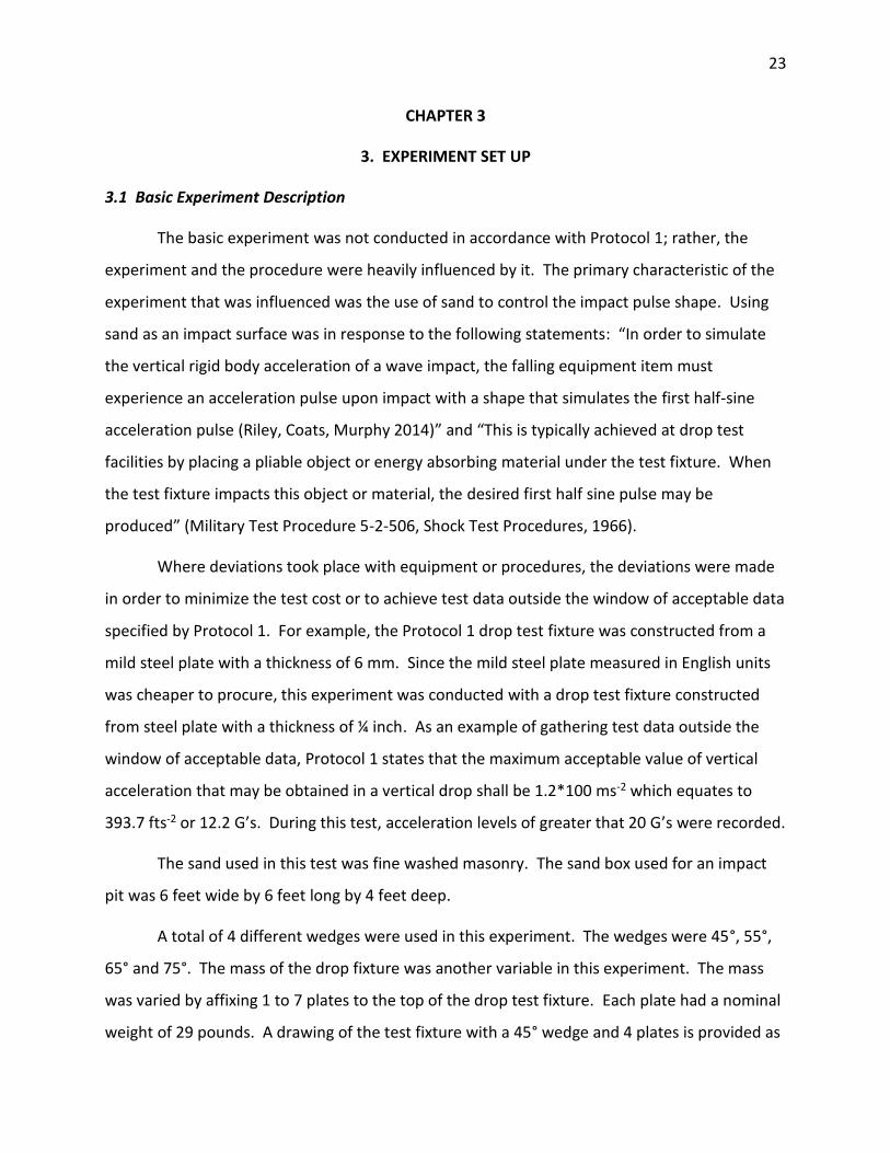
The basic experiment was not conducted in accordance with Protocol 1; rather, the

experiment and the procedure were heavily influenced by it. The primary characteristic of the

experiment that was influenced was the use of sand to control the impact pulse shape. Using

sand as an impact surface was in response to the following statements: “In order to simulate

the vertical rigid body acceleration of a wave impact, the falling equipment item must

experience an acceleration pulse upon impact with a shape that simulates the first half-sine

acceleration pulse (Riley, Coats, Murphy 2014)” and “This is typically achieved at drop test

facilities by placing a pliable object or energy absorbing material under the test fixture. When

the test fixture impacts this object or material, the desired first half sine pulse may be

produced” (Military Test Procedure 5-2-506, Shock Test Procedures, 1966).

Where deviations took place with equipment or procedures, the deviations were made

in order to minimize the test cost or to achieve test data outside the window of acceptable data

specified by Protocol 1. For example, the Protocol 1 drop test fixture was constructed from a

mild steel plate with a thickness of 6 mm. Since the mild steel plate measured in English units

was cheaper to procure, this experiment was conducted with a drop test fixture constructed

from steel plate with a thickness of ¼ inch. As an example of gathering test data outside the

window of acceptable data, Protocol 1 states that the maximum acceptable value of vertical

acceleration that may be obtained in a vertical drop shall be 1.2*100 ms-2 which equates to

393.7 fts-2 or 12.2 G’s. During this test, acceleration levels of greater that 20 G’s were recorded.

The sand used in this test was fine washed masonry. The sand box used for an impact

pit was 6 feet wide by 6 feet long by 4 feet deep.

A total of 4 different wedges were used in this experiment. The wedges were 45°, 55°,

65° and 75°. The mass of the drop fixture was another variable in this experiment. The mass

was varied by affixing 1 to 7 plates to the top of the drop test fixture. Each plate had a nominal

weight of 29 pounds. A drawing of the test fixture with a 45° wedge and 4 plates is provided as

24

Figure 5. The complete drawing package used to fabricate the drop test fixture is included in

this document as appendix A.

Figure 5. Drop Test Fixture With 45° Wedge

3.2 Detailed Experiment Description

For this experiment, the drop heights selected were 3 feet, 5 feet, 7 feet and 9 feet. The

test fixture was raised to the specified drop height via a bridge crane. The height of the drop

was measured by means of a length of cord cut to length and taped to the bottom of the

wedge. A photograph of the test fixture suspended above the sand box is provided as Figure 6.

25

Figure 6. Drop Test Fixture Suspended Above The Sand Box.

The test fixture was dropped from the hook of a bridge crane. A shackle was attached

to the crane hook. Beneath the shackle was a load cell that continually sensed the weight of

the test fixture. Beneath the load cell was a quick release mechanism that was activated by

pulling a lanyard. Prior to attaching the test fixture to the quick release mechanism, test

personnel raised the quick release from the floor and then zeroed the weight thus eliminating

the weight of the quick release from the displayed weight of the test fixture. A photograph of

the load cell and quick release mechanism used in testing is provided as Figure 7.

26

Figure 7. Load Cell and Quick Release Mechanism Used During Testing.

A Silicon Designs model 50 accelerometer and a MicroStrain GX3 Inertial Measurement

Unit was attached to the top plate. These sensors were used to sense the orientation of the

fixture prior to release and to sense the acceleration of the fixture throughout the test event.

Prior to dropping the fixture, test personnel would ensure that the pitch and roll angles of the

fixture were at 0° ± 1°. A bi-axial strain gauge was attached to each side of the wedge that

sensed strain during impact. Strain data was collected for informational purposes only. All of

the data was collected and stored using a National Instruments CompactRIO data acquisition

and signal conditioning system. Following each drop, the electronic data was stored and the

penetration depth into the sand was noted and recorded. The wedge was then lifted from the

sand; the sand in the immediate area of the impact was turned over several times with a shovel

to reduce the potential effects of sand compaction and then the sand was leveled. The wedge

was then dusted off, and test personnel prepared for the next test drop. A photograph of the

45° wedge fixture immediately after coming to rest in the sand box is provided as Figure 8.

27

Figure 8. 45° Wedge Fixture Following A Drop Into The Sand Box

A total of 112 individual test conditions existed for this experiment (4 wedges x 7 weight

plates x 4 drop heights = 112 test conditions). To minimize cost, only one drop at each of the

112 separate test conditions was initially authorized. At the conclusion of these 112 drops,

further authorization was granted to increase the number of drops from 1 at each test

condition to a total of 5 drops at each test condition. With this additional authorization, a total

of 560 drops would be completed. However, only the additional drops for the 45° wedge were

completed, which resulted in another 112 drops being performed (1 wedge angle (45°) x 7

weight plates x 4 drop heights x 4 drops = 112 drops). These additional drops combined with

the initial 112 drops resulted in a total of 224 drops completed. One of the 224 drops had an

instrumentation problem that was not discovered until test completion. As a result, data was

analyzed from a total of 223 valid drops. These two series of drop tests resulted in a completed

test matrix of 5 drops for the 45° wedge and only 1 drop at each of the other test conditions for

the 55° wedge, the 65° wedge and the 75° wedge.

One feature that was added to the top plate of the test fixture following the first series

of 112 drops was a symmetrical and center mounted aluminum plate that protected the sensor

28

package from potential damage from a falling shackle. This aluminum plate and mounting

hardware weighed a total of 3.8 pounds. This additional weight was noted in the total weight

of the fixture.

29

CHAPTER 4

4. EXPERIMENT RESULTS

4.1 Data Analysis

Data generated during this experiment was analyzed using the modal decomposition

method (Riley, Coats, Murphy 2014). Raw data was obtained from the cRIO system in its raw

TDMS file format. It was then converted to a text file using a file conversion utility written by

personnel at NSWCCD DN Code 835. The text file was then imported into MS Excel, and all

headers were removed. The resulting file was then saved as a Comma Separated Variables

(CSV) file. The CSV file was then imported into a software package identified as UERDTools

(Mantz, Costanzo, Howell III, Ingler, Luft, Okano). UERDTools is a software package that was

written by personnel at Naval Surface Warfare Center, Carderock in West Bethesda, Maryland

that was designed to analyze wave forms generated by underwater explosive events. For this

experiment, UERDTools was used to demean, zoom in on, and to perform 10 Hz low pass

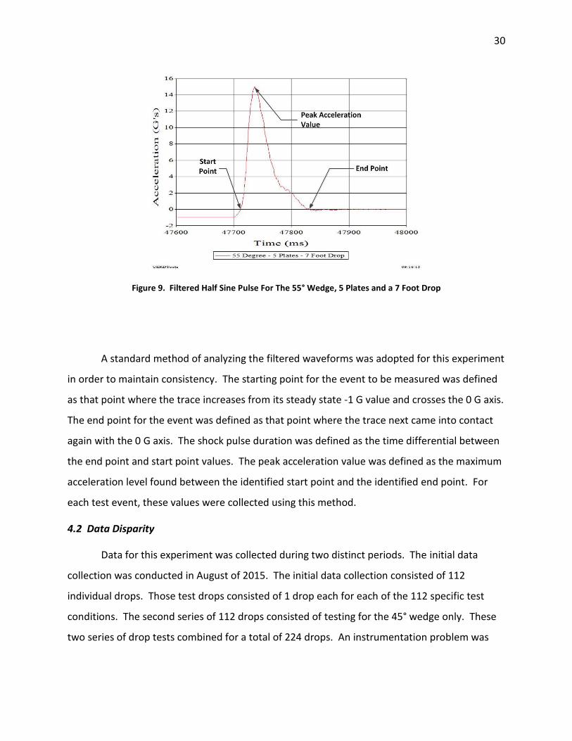
filtering of the test event. A sample of a filtered waveform event that was generated by

dropping the 55° wedge loaded with seven plates from a height of 7 feet is provided as Figure

9.

30

Figure 9. Filtered Half Sine Pulse For The 55° Wedge, 5 Plates and a 7 Foot Drop

A standard method of analyzing the filtered waveforms was adopted for this experiment

in order to maintain consistency. The starting point for the event to be measured was defined

as that point where the trace increases from its steady state -1 G value and crosses the 0 G axis.

The end point for the event was defined as that point where the trace next came into contact

again with the 0 G axis. The shock pulse duration was defined as the time differential between

the end point and start point values. The peak acceleration value was defined as the maximum

acceleration level found between the identified start point and the identified end point. For

each test event, these values were collected using this method.

4.2 Data Disparity

Data for this experiment was collected during two distinct periods. The initial data

collection was conducted in August of 2015. The initial data collection consisted of 112

individual drops. Those test drops consisted of 1 drop each for each of the 112 specific test

conditions. The second series of 112 drops consisted of testing for the 45° wedge only. These

two series of drop tests combined for a total of 224 drops. An instrumentation problem was

31

noted with one of the test drops but was not discovered until after the test was complete.

Therefore, data was obtained for a total of 223 valid drops.

For each series of drops, the same equipment, the same fixtures, the same

instrumentation and the same personnel were used to collect the data. During the period

between the experiments, August 2015 and June 2016, the impact sand box remained inside

the waterfront facility of Naval station Norfolk, Building V-47 protected from the effects of rain

and snow.

The data from both data collection periods were analyzed as described in the above

section of this document. All of the data from the 2 series of drop tests were merged into a

single file and sorted by wedge angle, number of plates and drop height. A small sample of the

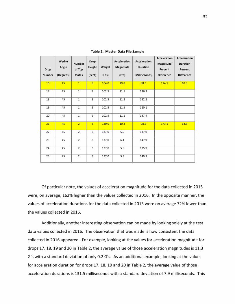
sorted master data file is provided as Table 2. Following the merging and sorting of data,

inspection of the master data file revealed an interesting trend. The data collected in August of

2015 consistently had a higher acceleration magnitude and consistently had a smaller

acceleration duration than the data collected in June of 2016. This trend can be seen in the

data tabulated in Table 2. Drop number 16 was performed on 8 August 2016. When analyzed,

this drop had an acceleration magnitude of 19.8 G’s. This acceleration magnitude was 174%

higher than the average value of drops 17, 18, 19 and 20. Drop number 16 also had an

acceleration duration of 88.5 milliseconds. This acceleration duration was only 67% of the

average value of drops 17, 18, 19 and 20. A complete listing of the raw data collected in this

effort is provided as appendix B.

32

Table 2. Master Data File Sample

Drop

Number

Wedge

Angle

(Degrees)

Number

of Top

Plates

Drop

Height

(Feet)

Weight

(Lbs)

Acceleration

Magnitude

(G's)

Acceleration

Duration

(Milliseconds)

Acceleration

Magnitude

Percent

Difference

Acceleration

Duration

Percent

Difference

16 45 1 9 104.0 19.8 88.5 174.5 67.3

17 45 1 9 102.5 11.5 136.3

18 45 1 9 102.5 11.2 132.2

19 45 1 9 102.5 11.5 120.1

20 45 1 9 102.5 11.1 137.4

21 45 2 3 130.0 10.3 98.5 173.1 64.5

22 45 2 3 137.0 5.9 137.0

23 45 2 3 137.0 6.1 147.9

24 45 2 3 137.0 5.9 175.9

25 45 2 3 137.0 5.8 149.9

Of particular note, the values of acceleration magnitude for the data collected in 2015

were, on average, 162% higher than the values collected in 2016. In the opposite manner, the

values of acceleration durations for the data collected in 2015 were on average 72% lower than

the values collected in 2016.

Additionally, another interesting observation can be made by looking solely at the test

data values collected in 2016. The observation that was made is how consistent the data

collected in 2016 appeared. For example, looking at the values for acceleration magnitude for

drops 17, 18, 19 and 20 in Table 2, the average value of those acceleration magnitudes is 11.3

G’s with a standard deviation of only 0.2 G’s. As an additional example, looking at the values

for acceleration duration for drops 17, 18, 19 and 20 in Table 2, the average value of those

acceleration durations is 131.5 milliseconds with a standard deviation of 7.9 milliseconds. This

33

calculation was performed for all sets of the 45° wedge data collected in 2016, and the average

of all standard deviation calculations for acceleration magnitude was only 0.2 G’s, and the

average of all standard deviation calculations for acceleration duration was only 8.6

milliseconds.

For the purposes of comparison, the standard deviations for all of the data for the 45°

wedge were calculated. In this case, when combining the 2015 and the 2016 45° wedge data,

the average standard deviation for acceleration magnitude rose to 2.4 G's, and the average

standard deviation for acceleration duration rose to 21.0 milliseconds.

Since there was no difference in any of the equipment or personnel that was used in

both the 2015 and 2106 drops, it is hypothesized that the sand dried during the year between

the two series of drop tests. This theory would stand to reason since the sand that was used in

this test was washed masonry sand and had some water in it for the 2015 test. Since the

impact box sat dormant and was not exposed to rain and snow for approximately 1 year, it had

time to dry. The absence of water could certainly explain why impact magnitudes in wet sand

had a higher magnitude than dry sand. It could also explain why the acceleration durations for

wet sand were smaller for wet sand than for dry sand.

4.3 Wedge Angle, Weight and Drop Height Effects Upon Acceleration Magnitude

4.3.1 Data Exclusion

Data for the 112 drops gathered in 2015 was plotted in order to determine trends. The

2016 data was not included in the plots because as discussed in section 4.2 of this document,

there is a noticeable disparity between the two data sets. This disparity could unduly influence

the plots and negatively influence the trend recognition process. Exclusion of the 2016 data set

from the plotting process was made simply to remove the possible effects of moisture content

in the sand as a possible variable. However, a set of empirical equations using a combination of

the 2015 data and the 2016 data has been provided and will be discussed later in this

document.

34

4.3.2 Wedge Angle Effects Upon Acceleration Magnitude

The effect of wedge angle upon acceleration magnitude was plotted by sorting the data

by wedge angle, drop height and then by the number of plates mounted to the test fixture. As

depicted in Figure 10, the plots of 3 foot drops represent roughly a horizontal pattern. The

exceptions to this pattern are the light blue 3 foot drop with one plate that has an unusually

high value associated with the 75° wedge and the orange 3 foot drop with 6 plates that had an

unusually low value associated with the 55° wedge.

Figure 10. Wedge Angle Versus Acceleration Magnitude For The 3 Foot Drop

Examination of the 5 foot drop data, the 7 foot drop data and the 9 foot drop data

revealed the effects of wedge angle upon acceleration magnitude becomes noticeably more

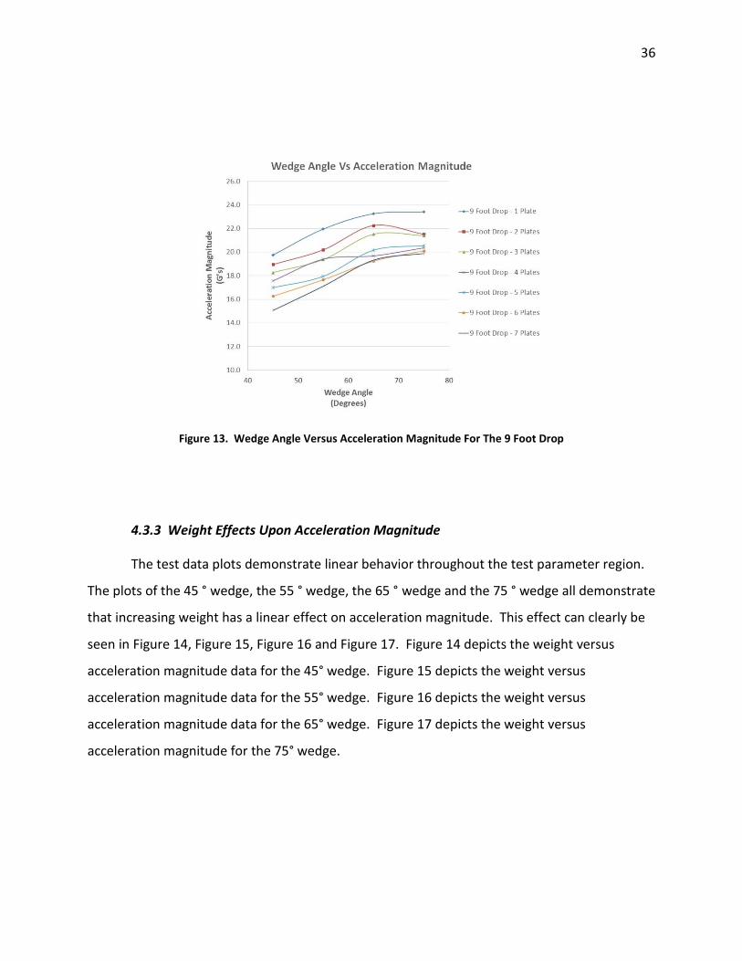
linear as the drop height increases. Figure 11 is a plot of the 5 foot drop data. Figure 12 is a

plot of the 7 foot drop data. This trend can be seen in Figure 13, which is a plot of the 9 foot

35

drop data. Most of the plots are parallel with the exception of the purple 9 foot drop with 4

plates.



36


4.3.3 Weight Effects Upon Acceleration Magnitude

The test data plots demonstrate linear behavior throughout the test parameter region.

The plots of the 45 ° wedge, the 55 ° wedge, the 65 ° wedge and the 75 ° wedge all demonstrate

that increasing weight has a linear effect on acceleration magnitude. This effect can clearly be

seen in Figure 14, Figure 15, Figure 16 and Figure 17. Figure 14 depicts the weight versus

acceleration magnitude data for the 45° wedge. Figure 15 depicts the weight versus



acceleration magnitude for the 75° wedge.

37

Figure 14. Weight Versus Acceleration Magnitude For The 45° Wedge


38



39

4.3.4 Drop Height Effects Upon Acceleration Magnitude

The test data plots indicate linear behavior. The plots of the 45° wedge, the 55° wedge,

the 65° wedge and the 75° wedge all demonstrate that increasing drop height has a linear

effect upon acceleration magnitude. This effect can clearly be seen in Figure 18, Figure 19,

Figure 20 and Figure 21. Figure 18 depicts the drop height versus acceleration magnitude data

for the 45° wedge. Figure 19 depicts the drop height versus acceleration magnitude for the 55°

wedge. Figure 20 depicts the drop height versus acceleration magnitude for the 65° wedge.

Figure 21 depicts the drop height versus acceleration magnitude for the 75° wedge.

Figure 18. Drop Height Versus Acceleration Magnitude For The 45° Wedge

40



41


4.4 Wedge Angle, Weight and Drop Height Effects Upon Acceleration Duration

4.4.1 Wedge Angle Effects Upon Acceleration Duration

The effect of wedge angle upon acceleration duration was plotted by sorting the data by

wedge angle, drop height and then by the number of plates mounted to the test fixture. As

depicted in Figure 22, the plots of 3 foot drops represent roughly a horizontal pattern. The

exceptions to this pattern are the blue 3 foot drop with one plate that has an unusually high

value associated with the 55° wedge and the orange 3 foot drop with 6 plates that also had an

unusually high value associated with the 55° wedge.

42

Figure 22. Wedge Angle Versus Acceleration Duration For The 3 Foot Drop

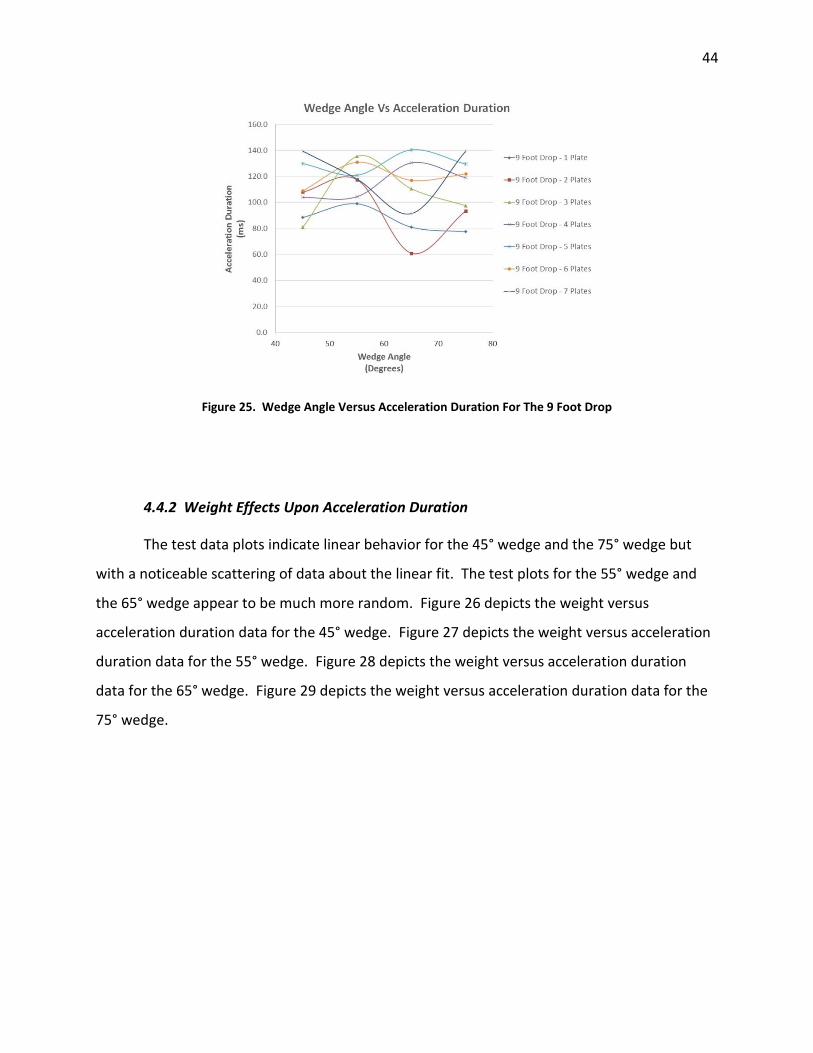
The effect of wedge angle upon acceleration duration became more random as the drop

height increased. This trend was noted in the 5 foot drop data, the 7 foot drop and the 9 foot

drop data. The randomness of the data was at its most extreme in the 9 foot drop data. A plot

of the 5 foot drop data is provided as Figure 23. A plot of the 7 foot drop data is provided as

Figure 24. A plot of the 9 foot drop data is provided as Figure 25.

43



44


4.4.2 Weight Effects Upon Acceleration Duration

The test data plots indicate linear behavior for the 45° wedge and the 75° wedge but

with a noticeable scattering of data about the linear fit. The test plots for the 55° wedge and

the 65° wedge appear to be much more random. Figure 26 depicts the weight versus

acceleration duration data for the 45° wedge. Figure 27 depicts the weight versus acceleration

duration data for the 55° wedge. Figure 28 depicts the weight versus acceleration duration

data for the 65° wedge. Figure 29 depicts the weight versus acceleration duration data for the

75° wedge.

45

Figure 26. Weight Versus Acceleration Duration For The 45° Wedge


46



47

4.4.3 Drop Height Effects Upon Acceleration Duration

The test data plots show random behavior. If a linear regression data fit was fitted

through the data in Figure 30 and in Figure 31, the slope of both of those lines would be

minimal. In fact, the slope of the line for the linear fit of data in Figure 30 was 0.867, and the

slope for the linear data fit in Figure 31 was 1.746. Figure 30 depicts the drop height versus

acceleration duration data for the 45° wedge. Figure 31 depicts the drop height versus

acceleration duration for the 75° wedge. Since the slope of the lines is minimal, this would

suggest that drop height was not a major contributing factor to acceleration duration.

One obvious factor to performing linear fits to the data in Figure 30 and Figure 31 was

the amount of error that would be observed about the linear data fit. For the linear fit for the

data in Figure 30, the standard error was 11.377. For the linear fit for the data in Figure 31, the

standard error was 17.3905. Since no other data trends are obvious in the data, it is assumed

that the data follows a linear trend with a large error about the best fit line.

Figure 30. Drop Height Versus Acceleration Duration For The 45° Wedge

48


Figure 32 and Figure 33 are provided for informational purposes. Figure 32 depicts the

drop height versus acceleration duration data for the 55° wedge. Figure 33 depicts the drop

height versus acceleration duration data for the 65° wedge

49



50

4.4.4 Acceleration Duration Data Dispersion

It is evident that there is much variation in the acceleration duration for each of the

plots shown above. Intuitively, one would think that for a given wedge angle and weight, such

as 65° with 2 plates as shown in Figure 33, that as drop height increases so would acceleration

duration. However, the exact opposite behavior has been noticed for this example. In this

particular case, a decrease of approximately 50 ms has been observed.

During the data analysis process of this effort, it was observed that there was little

consistency in the time differential from the transition point until the time where the curve

crossed the zero axis at the end point. For the purposes of this document, the transition point

is defined as being where the steep slope of the rear half of the sinusoidal acceleration pulse

begins to flatten out. Figure 34 illustrates the location of a transition point in data from a

sample full-scale craft, rough water test that was not part of this effort. The selection of Figure

34 was only to provide the reader with a clear example of an easily defined transition point. In

most cases, the data from this effort did not have such clearly defined transition points. This

observation can be easily seen in Figure 9 where determining the location of the transition

point would require some subjective judgment. The inconstancies within the acceleration

duration data for this effort were chiefly located in the region from the transition point to the

time where the curve crossed the zero axis at the end point. In some cases, the time from the

transition point to the end point was up to 50 ms longer than expected. No reason for this

disparity was observed.

51

Figure 34. Transition Point Illustration

When looking at full-scale planing craft motion data, it is not uncommon to see

acceleration pulse durations ranging from 75-200 ms. This could happen for a variety of

reasons: rolling or pitching at the time of impact, the size variations in the waves, differences in

the impact velocity, etc. Considering this with respect to the drop tests performed, given that

there was no apparatus to maintain zero pitch or roll during the drop, given that there may

have been variations in the sand surface between drops, and understanding that the sand

consistency would likely vary with depth, it is not unlikely that there should be variations in

duration from one drop to the next.

4.5 Compliance With Protocol One

Since the test that was performed in this effort was based upon the test method

described in Protocol One, it is not surprising that some of the time history curves generated

could fit within the allowable region of a valid Protocol One compliant test. Where there was

discrepancy with Protocol One, it was due to exceeding the maximum acceleration magnitude

limit. The maximum acceleration magnitude allowed in Protocol One is 12.2 G’s, and many of

the time history curves generated in this effort exceeded this maximum level. An example of

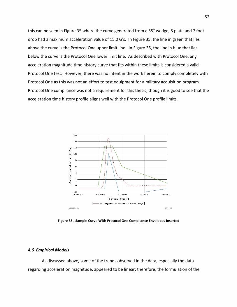
52

this can be seen in Figure 35 where the curve generated from a 55° wedge, 5 plate and 7 foot

drop had a maximum acceleration value of 15.0 G’s. In Figure 35, the line in green that lies

above the curve is the Protocol One upper limit line. In Figure 35, the line in blue that lies

below the curve is the Protocol One lower limit line. As described with Protocol One, any

acceleration magnitude time history curve that fits within these limits is considered a valid

Protocol One test. However, there was no intent in the work herein to comply completely with

Protocol One as this was not an effort to test equipment for a military acquisition program.

Protocol One compliance was not a requirement for this thesis, though it is good to see that the

acceleration time history profile aligns well with the Protocol One profile limits.

Figure 35. Sample Curve With Protocol One Compliance Envelopes Inserted

4.6 Empirical Models

As discussed above, some of the trends observed in the data, especially the data

regarding acceleration magnitude, appeared to be linear; therefore, the formulation of the

53

empirical models for acceleration magnitude and acceleration duration would be accomplished

using linear regression techniques. The linear regression tool selected for this task was the

MVREGRESS tool located in MATLAB. Two separate sets of empirical models were generated.

One set of empirical models was generated that would model only the first 112 drops

conducted in 2015. The second set of empirical models was generated using the entire data

set, consisting of 2015 and 2016 data that would model all 224 drops conducted. Equations 1

and 2 model the 112 drops conducted in 2015. Equations 3 and 4 model all 224 drops

conducted in both 2015 and 2016. In both sets of equations the following variables are defined

as:

A = Wedge angle, measured in degrees;

W = Drop test fixture weight, measured in pounds;

H = Drop height, measured in feet;

Acceleration Magnitude, measured in G’s;

Acceleration Duration, measured in milliseconds.

For 112 drops:

(Eqn 1)

(Eqn 2)

For 224 drops:

(Eqn 3)

(Eqn 4)

Both sets of equations were evaluated and compared to the actual data values

collected. Table 3 summarizes the statistical results of empirical model comparison with the

collected test data. Equations 1 and 2 were compared with the test data for the 112 drops

conducted in 2015. Equations 3 and 4 were compared with the test data for all 224 drops

54

conducted in 2015 and 2016. As can be observed in Table 3, equations 1 and 2 demonstrate

greater statistical accuracy than equations 3 and 4. The greater statistical error demonstrated

with these models can be attributed to the data disparity discussed earlier.

Table 3. Empirical Model Statistical Summary

Equation Average Error

Standard

Deviation Maximum Error Minimum Error

Eqn 1 0.0 0.8 2.0 -2.3

Eqn 2 0.0 14.2 38.8 -40.6

Eqn 3 0.0 2.2 5.1 -3.6

Eqn 4 0.0 19.2 55.0 -54.2

Another check of the accuracy of the derived equations would be to plot the actual

results versus the predicted results. The results were segregated by drop height. The decision

to group the data in this method was based on the assumption that the error within the data

would grow smaller as drop height increased. Figure 36 depicts the plotted data for equation 1,

which predicts acceleration magnitude. Figure 37 depicts the plotted data for equation 2,

which predicts acceleration duration. Equations 1 and 2 were selected for this accuracy check

because they demonstrated lower error values than equations 3 and 4.

Once the data was plotted, a least squares curve fit was applied to each group of data.

A slope of 1 would indicate a perfect math model prediction. A slope greater that 1 would

indicate that the math model over predicts the results. A slope less than 1 would indicate that

the math model under predicts the results. Additionally, the R squared value was calculated for

each least squares fit to determine the goodness of fit.

55

The plotted data in Figure 36 demonstrated linear patterns. An interesting observation

is that the goodness of fit increased from 0.41 for the 3 foot drop to 0.91 for the 9 foot drop.

This confirms the original assumption discussed above. Conversely, the math model begins to

more consistently under predict as drop height increases. This can be observed with a slope for

the least squares fit of 0.84 for the 3 foot drop and a slope for the least squares fit of 0.67 for

the 9 foot drop.

Figure 36. Acceleration Magnitude, 112 Drops Actual Vs Predicted Results

No further analysis was performed with equation 2 since no data patterns were

observed in Figure 37.

56

Figure 37. Acceleration Duration, 112 Drops Actual Vs Predicted Results

4.7 Application Example

Equations 1 and 2 can be used by interested parties to simulate, in the laboratory, single

impact events based upon the measured rough water performance of a craft in a seaway. For

example, suppose that a marine radio manufacturer has built a prototype Very High Frequency

(VHF) radio and, with it, a specialty mounting system designed to mitigate the effects of the

wave slamming that the radio will be subjected to during rough water operations. The VHF

radio manufacturer wants to know how efficient the mounting system is in reducing shock. The

VHF radio manufacturer does not have access to craft or personnel that can perform a rough

water test that will allow them the opportunity to learn this information under real world

conditions, but assume that they do have access to some rough water data for a particular

craft. After review of the rough water test data, the VHF radio manufacturer has determined

that the worst case shock that their system will see in a particular craft would be at an

acceleration level of 15.4 G’s and at an acceleration duration of 120 milliseconds.

Assume that the prototype VHF radio weighs 4 pounds and that the corresponding

shock absorbing mount weighs 9 pounds. This combined system weighs 13 pounds. Also

57

suppose that the radio manufacturer has a warehouse with a high enough ceiling to allow a

series of 6 foot drops from a roof truss. It is also assumed that the radio manufacturer has

access to appendix B of this thesis and, as such, knows the weight of all of the wedges and plate

combinations. With these pieces of information and by using equations 1 and 2, the radio

manufacturer can modify appendix C into a simple spreadsheet and select a wedge angle,

fixture weight combination that when dropped from a 6 foot height can produce the shock

environment that is targeted. In this particular case, selecting the 75° wedge with 4 plates and

the mounted radio system (total weight = 170 pounds + 13 pounds = 183 pounds) and dropping

it from a height of 6 feet can produce an acceleration magnitude of 15.4 G’s and an

acceleration duration of 112.5 milliseconds. The radio manufacturer can install an

accelerometer on the top deck of the fixture and upon the radio itself. By comparing the data

generated by the two accelerometers during a series of drop tests, the radio manufacturer can

cheaply determine the effectiveness of the shock absorbing mount before subjecting it to an

expensive and time consuming rough water test. After determining what combination of

wedge angle, weight and drop height to use, it would be wise if the radio manufacturer

performed a series of tuning drops where the manufacturer would tune the three parameters

in order to get as close to the desired acceleration level and acceleration magnitude as possible.

58

CHAPTER 5

5. CONCLUSIONS AND RECOMMENDATIONS

It was observed that the effect of wedge angle upon acceleration magnitude was

roughly linear. It was also observed that the effect of wedge angle upon acceleration duration

was random and the randomness became more pronounced as the drop height increased.

It was observed that the effect of weight upon acceleration magnitude was linear

throughout the test variable region. It was also observed that the effect of weight upon

acceleration duration was linear but with a large error about a best fit line.

It was observed that the effect of drop height upon acceleration magnitude was linear

throughout the test variable region. It was also observed that the effect of drop height upon

acceleration duration was roughly a horizontal line with a large error about the best fit line.

It was observed that a plot of actual versus predicted acceleration magnitudes results in

linear behavior. When these results were sorted by drop height, the error became smaller as

the drop height increased. It was also observed that the slope of a best fit line through these

data plots resulted in a decreasing slope as drop height increased. This trend would suggest

that the math model for acceleration magnitude increasingly under predicts as drop height

increases.

It was observed that a plot of actual versus predicted acceleration durations resulted in

no visibly discernable pattern.

As demonstrated in section 4.7, equations 1, 2, 3 and 4 can be used as a tool to

customize a drop test that can simulate a single wave impact. It should be noted that these

equations are only valid in the regions of weight from 110 pounds to 297 pounds, regions of

drop heights from 3 feet to 9 feet, regions of wedge angle from 45° to 75° and in a consistent

sand moisture content. It should also be noted that for the 112 drops conducted in 2015, only

one drop at each test condition was conducted. Even though the data set was expanded to 5

drops in each test condition for the 45° wedge, these additional test drops demonstrated that

there was disparity in test results when the tests were conducted with different sand

59

conditions. Therefore, it is recommended that the presented equations be used as a general

guide to test personnel designing a drop test to simulate wave impacts. It is recommended that

test personnel conduct preliminary drops to verify and tune the performance of their test setup

prior to conducting a specific test.

There are potential areas where the results of this research could be improved and

refined. As discussed above, an issue noted during the execution of this thesis effort was the

accuracy of the empirical models. The generation of these models was based on limited data.

In the case of equations 1 and 2, 112 valid data points were used for model generation. In the

case of equations 2 and 3, 223 valid data points were used for model generation. A way to

refine the accuracy of empirical models by using more data would be for an interested party to

conduct further tests based upon the methods, drawings and procedures provided within this

thesis.

Another issue that should be investigated is determining how the moisture content of

the sand affects the peak acceleration magnitude and acceleration duration upon impact. A

method for measuring the moisture content should be included in the test procedure. This

information should be collected and then integrated into the empirical model generation.

60

REFERENCES

GeoMagic Design Expert, Version 12, 333 Three D Systems Circle, Rock Hill, SC 29730

National Instruments cRIO Post Processing Data Script, NSWCCD, Code 835

Riley, Michael R., Haupt, Kelly D., Jacobson, Donald R. (2010). “A Generalized Approach and

Interim Criteria for Computing A1/n Accelerations Using Full-Scale High-Speed Craft Trials Data”,

Naval Surface Warfare Center Carderock Division Report NSWCCD-23-TM-2010/13, April 2010

Savitsky, Daniel and Brown P.W. (October 1976). “Procedures for Hydrodynamic Evaluation of

Planing Hulls in Smooth and Rough Water”, Marine Technology, Volume 13, No. 4.

Riley, Michael R., Haupt, Kelly D., Jacobson, Donald R. (2012). “A Deterministic Approach For

Characterizing Wave Impact Response Motions Of A High-Speed Planing Hull”, Naval Surface

Warfare Center Carderock Division Report NSWCCD-23-TM-2012/05, January 2012

Riley, Michael R., Coats, Dr. Timothy W., Murphy, Heidi (2014). “Acceleration Response Mode

Decomposition For Quantifying Wave Impact Load In High Speed Planing Craft”, Naval Surface

Warfare Center Carderock Division Report NSWCCD-23-TR-2014/007, April 2014

Protocol 1 (2014). “Maritime Whole Body Vibration, Shock Mitigating Seat Test”, PQQ

Reference JK6KHJ8427, United Kingdom Ministry Of Defense, 08/01/2014

UERDTools, Version 4.4. Mantz, Paul, Costanzo, Fredrick, Howell III, Jamie, Ingler, Dave, Luft,

Eric, Okano, Steve, Naval Surface Warfare Center, Carderock Division, Underwater Explosion

and Research Development, 9500 MacArthur Boulevard, West Bethesda, MD 20817-5700

MATLAB, Version 8.2, MathWorks Inc., Natick, Massachusetts

Military Test Procedure 5-2-506, Shock Test Procedures, U.S. Army Test and Evaluation

Command, White Sands Missile Range, New Mexico, December 1966.

61

Appendix A - Technical Drawing Package of Drop Fixture

CH

ECK

ED

B

John

Bar

ber

REV

DES

CR

IPTI

ON

ZON

EAP

PRO

VED

DAT

E

B

4

C

14

DAT

E

APPR

OVE

D

REV

ISIO

NS

2

MFG

D

REV

D

DW

G N

O.

QA

13

SHEE

T

1 M

ay 2

015

A

FSC

M N

O.

A

2

C

SIZE

3

DR

AW

N

SK

-001

SCAL

E

C

Dro

p Fi

xtur

e - 4

5 D

egre

e W

edge

NO

TES

1. A

ssem

bled

Wei

ght -

183

Pou

nds

1 of

3

DES

CR

IPTI

ON

D

REV

CH

ECK

ED

2

SIZE

SCAL

E

APPR

OVE

D

4

John

Bar

ber

DR

AW

N

A

CC B

4

D

DAT

E

1 M

ay 2

015

REV

DW

G N

O.

SK

-001

1

3

REV

ISIO

NS

QA

SHEE

T

A

C

2

1

B

3

FSC

M N

O.

APPR

OVE

D

DAT

E

MFG

ZON

E

Dro

p Fi

xtur

e - 4

5 D

egre

e W

edge

2 of

3

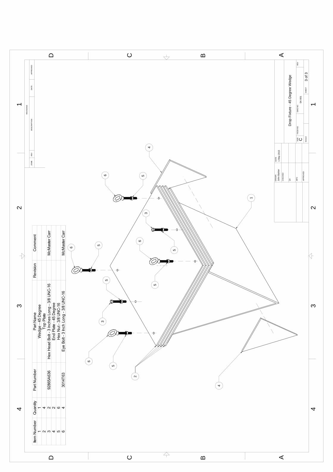
1

3

34

4

5

5

5

5

5

2

6

56

6

6

Item

Num

ber

Qua

ntity

Par

t Num

ber

Par

t Nam

eR

evis

ion

Com

men

t1

1W

edge

- 45

Deg

ree

24

Top

Pla

te3

292

865A

636

Hex

Hea

d B

olt -

3 In

ches

Lon

g - 3

/8 U

NC

-16

McM

aste

r Car

r4

2E

nd P

late

- 45

Deg

ree

56

Hex

Nut

- 3/

8 U

NC

-16

64

3014

T63

Eye

Bol

t - 3

Inch

Lon

g - 3

/8 U

NC

-16

McM

aste

r Car

r

DAT

ED

RA

WN

1 M

ay 2

015

4

REV

C

1SC

ALE

DES

CR

IPTI

ON

APPR

OVE

DC

APPR

OVE

D

3

John

Bar

ber

SK

-001

B

1

SHEE

T

3

REV

ISIO

NS

CH

ECK

ED

D

QA

MFG

SIZE

REV

4

2

D

B

ZON

E

2

DAT

E

AC

A

DW

G N

O.

FSC

M N

O.D

rop

Fixt

ure

- 45

Deg

ree

Wed

ge

3 of

3

1

B

CH

ECK

ED

MFG

REV

C

REV

ISIO

NS

C

John

Bar

ber

APPR

OVE

D

DW

G N

O.

3

ZON

ED

ATE

APPR

OVE

D

QA

SCAL

E

2 2

FSC

M N

O.

34

A

D

SK

-008

DR

AW

N

A

D

4

B

1

DAT

E

2 M

ay 2

015

SIZE C

REV

DES

CR

IPTI

ON

SHEE

T

Not

es

1. A

ssem

bled

Wei

ght -

174

Pou

nds

Dro

p Fi

xtur

e - 5

5 D

egre

e W

edge 1 of

3

DES

CR

IPTI

ON

REV

2

A

DW

G N

O.

C

DAT

E

C

SK

-008

SHEE

T

MFG

QA

APPR

OVE

D

2

D

DR

AW

N

B

APPR

OVE

D

AC

HEC

KED

FSC

M N

O.

B

SCAL

E

REV

ISIO

NS

3

ZON

E

14

C

DAT

E

2 M

ay 2

015

John

Bar

ber

REV

34

D

SIZE

1

Dro

p Fi

xtur

e - 5

5 D

egre

e W

edge

2 of

3

1

2

3

4

4

5

5

5

5

5

5

6

6

6

6

3

Item

Num

ber

Qua

ntity

Par

t Num

ber

Par

t Nam

eR

evis

ion

Com

men

t1

1W

edge

- 55

Deg

rees

24

Top

Pla

te3

292

865A

636

Hex

Hea

d B

olt -

3/8

Inch

- 16

UN

C -

3 In

ches

Lon

gM

cMas

ter C

arr

42

End

Pla

te -

55 D

egre

es5

6H

ex N

ut -

3/8

Inch

- 16

UN

C6

430

14T

63E

ye B

olt -

3/8

Inch

- 16

UN

C -

3 In

ch L

ong

McM

aste

r Car

r

QA

DR

AW

N

4

2

D A

3

B

SCAL

E

SIZE

C

REV

ISIO

NS

CSH

EET

2 M

ay 2

015

1

B

D C A

ZON

ED

ESC

RIP

TIO

NR

EV

FSC

M N

O.

APPR

OVE

D

CH

ECK

ED

DAT

E

1

MFG

APPR

OVE

D

23

4

DW

G N

O.

SK

-008

REV

John

Bar

ber

DAT

E

Dro

p Fi

xtur

e - 5

5 D

egre

e W

edge 3 of

3

DES

CR

IPTI

ON

MFG

D

2

C

DR

AW

N

A

SHEE

T

SK

-011

DAT

E

APPR

OVE

D

C

3

ZON

E

4

2

31

SIZE

B

REV

ISIO

NS

John

Bar

ber

C

1

APPR

OVE

D

B

D

3 M

ay 2

015

A

DAT

E

4

FSC

M N

O.

SCAL

E

CH

ECK

ED

REV

DW

G N

O.

QA

REV

Dro

p Fi

xtur

e - 6

5 D

egre

e W

edge

NO

TES

1. A

ssem

bled

Wei

ght -

167

Pou

nds

1 of

3

REV

ISIO

NS

322

AC BB

SHEE

T

A

MFG

D

REV

John

Bar

ber

DW

G N

O.

APPR

OVE

D

3 M

ay 2

015

4SC

ALE

D

FSC

M N

O.

4

APPR

OVE

D

QA

DR

AW

N

DAT

E

C

1

3

ZON

E

SK

-011

DES

CR

IPTI

ON

CSIZE

1

CH

ECK

ED

DAT

E

REV

Dro

p Fi

xtur

e - 6

5 D

egre

e W

edge

2 of

3

1

2 3

3

4

4

5

5

5

5

5

5

6

6

6

6

Item

Num

ber

Qua

ntity

Par

t Num

ber

Par

t Nam

eR

evis

ion

Com

men

t1

1W

edge

- 65

Deg

ree

24

Top

Pla

te3

2E

nd P

late

42

9286

5A63

6H

ex H

ead

Bol

t - 3

/8 U

NC

-16

- 3 In

ches

Lon

gM

cMas

ter C

arr

56

Hex

Nut

- 3/

8 U

NC

-16

64

3014

T63

Eye

Bol

t - 3

/8 U

NC

-16

- 3 In

ches

Lon

gM

cMas

ter C

arr

DR

AW

N

4

C

REV

ZON

E

CH

ECK

ED

QA

MFG

DAT

E

B

SHEE

T

DW

G N

O.

SK

-011

DAT

E

John

Bar

ber

APPR

OVE

D

D

AD

4

APPR

OVE

D

3 M

ay 2

015

2

REV

ISIO

NS1

23 3

REV

DES

CR

IPTI

ON

SCAL

E

A

FSC

M N

O.

C

B

1

SIZE

C

Dro

p Fi

xtur

e - 6

5 D

egre

e W

edge

3 of

3

1

APPR

OVE

D

SK

-014

APPR

OVE

D

3

2

DAT

ER

EV

DR

AW

N

A

SCAL

E

MFG

3

REV

FSC

M N

O.

2

John

Bar

ber

D

SHEE

T

A

DES

CR

IPTI

ON

DW

G N

O.

DAT

E

SIZE

B

REV

ISIO

NS

4

ZON

E

4

CC

C

QA

10 M

ay 2

015

1

CH

ECK

ED

BD

NO

TES

1. A

ssem

bled

Wei

ght -

164

Pou

nds

Dro

p Fi

xtur

e - 7

5 D

egre

e W

edge

1 of

3

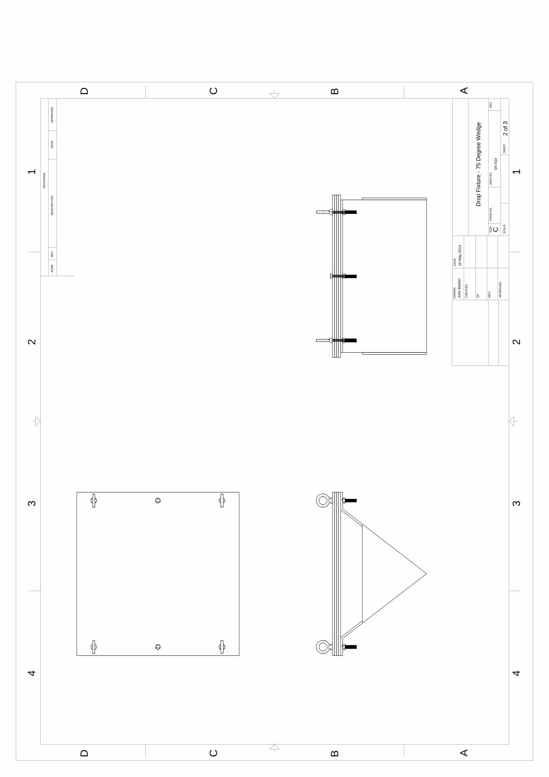
A

SCAL

E

1

ZON

ED

ATE

John

Bar

ber

FSC

M N

O.

CH

ECK

ED

SK

-014

C

APPR

OVE

D

4

REV

ISIO

NS

B

REV

DD

A

3

DW

G N

O.

MFG

DR

AW

N

DES

CR

IPTI

ON

APPR

OVE

D

4

REV

C

10 M

ay 2

014

2

BC

SIZE

3

DAT

E

1

QA

SHEE

T

2

Dro

p Fi

xtur

e - 7

5 D

egre

e W

edge

2 of

3

1

23

3

4

4

55

5

55

5

6

6

6

6

Item

Num

ber

Qua

ntity

Par

t Num

ber

Par

t Nam

eR

evis

ion

Com

men

t1

1W

edge

- 75

Deg

ree

24

Top

Pla

te3

2E

nd P

late

- 75

Deg

rees

42

9286

5A63

6H

ex H

ead

Bol

t - 3

/8 -1

6 U

NC

x 3

Inch

es L

ong

McM

aste

r Car

r5

6H

ex N

ut -

3/8

- 16

UN

C6

430

14T

63E

ye B

olt

- 3/8

- 16

UN

C x

3 In

ch L

ong

McM

aste

r Car

r

C

DW

G N

O.1

FSC

M N

O.

ZON

E

B

SCAL

E

C

C

D

DAT

E

4

John

Bar

ber

B

3

APPR

OVE

D REV

CH

ECK

ED

REV

1

SIZE

SHEE

T

MFG

D

REV

ISIO

NS

3

SK

-014

A

24

DR

AW

N

DES

CR

IPTI

ON

A

2

DAT

E

QA

10 M

ay 2

015

APPR

OVE

D

Dro

p Fi

xtur

e - 7

5 D

egre

e W

edge

3 of

3

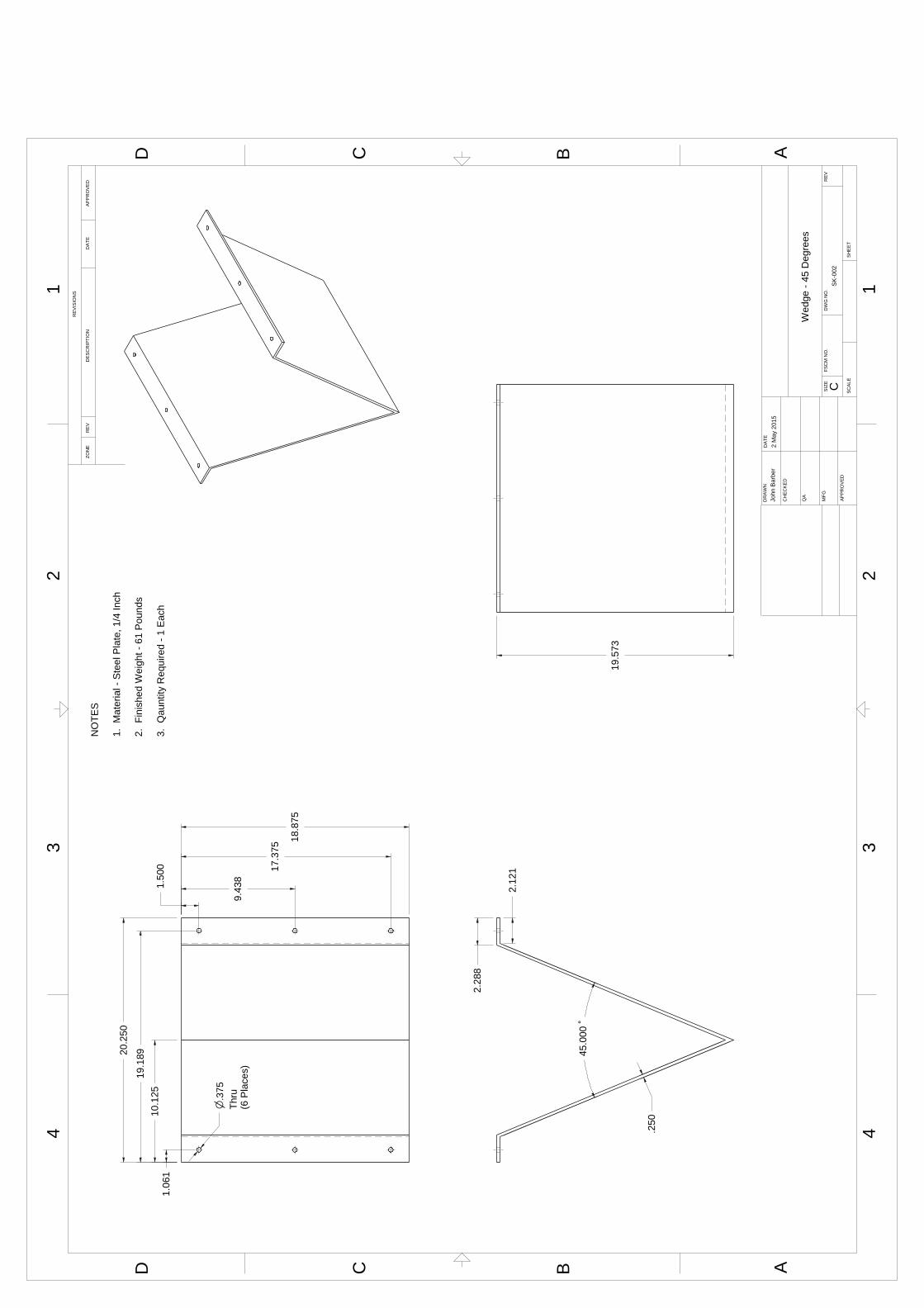
45.0

00 ˚

.250

2.28

8

2.12

1

20.2

50

1.06

110

.125

19.1

89

1.50

0

9.43

8

17.3

75

18.8

75

n.3

75Th

ru(6

Pla

ces)

19.5

73

SIZE

2 M

ay 2

015

3

SK

-002

MFG

3

B

SHEE

T

John

Bar

ber

B

REV

D

4

2

C

CH

ECK

ED

DAT

E

A

2

DW

G N

O.

DAT

E

FSC

M N

O.

1SC

ALE

ZON

ER

EV

QA

1

C

REV

ISIO

NS

DR

AW

N

D A

APPR

OVE

D

C

APPR

OVE

D

4

DES

CR

IPTI

ON

NO

TES

1. M

ater

ial -

Ste

el P

late

, 1/4

Inch

2. F

inis

hed

Wei

ght -

61

Pou

nds

3. Q

aunt

ity R

equi

red

- 1 E

ach

Wed

ge -

45 D

egre

es

2.27

3

2.12

1

.250

55.0

00 ˚

1.06

110

.125

19.1

89

20.2

50

1.50

0

9.43

8

17.3

75

18.8

75

n.3

75Th

ru(6

Pla

ces)

15.6

25

SK

-009

A

1

4SH

EET

DW

G N

O.

D

B

APPR

OVE

D

2 M

ay 2

015

DAT

EZO

NE

A

SCAL

EAP

PRO

VED

QAJohn

Bar

ber

C

34

REV

C

D

REV

ISIO

NS

FSC

M N

O.

SIZE

C

MFG

2

DR

AW

N

3

DES

CR

IPTI

ON

2

B

CH

ECK

ED

DAT

E

REV

1

Wed

ge -

55 D

egre

es

NO

TES

1. M

ater

ial -

Ste

el P

late

, 1/4

Inch

2. F

inis

hed

Wei

ght -

52

Pou

nds

3. Q

uant

ity R

equi

red

- 1 E

ach

65.0

00 ˚

.250

2.25

8

2.12

1

1.06

1

10.1

25

19.1

89

20.2

50

1.50

0

9.43

8

17.3

75

18.8

75

n.3

75Th

ru(6

Pla

ces)

12.8

13

QA

3

MFG

2

ZON

E

D

DES

CR

IPTI

ON

3

John

Bar

ber

B

4

1

REV

C

SIZE

DW

G N

O.

B

DAT

E

AD

RA

WN

APPR

OVE

D

CH

ECK

ED

2

1

REV

SHEE

T

C

D C

4

4 M

ay 2

015

SK

-012

FSC

M N

O.

REV

ISIO

NS

APPR

OVE

D

DAT

E

A

SCAL

E

Wed

ge -

65 D

egre

es

NO

TES

1. M

ater

ial -

Ste

el P

late

, 1/4

Inch

2. F

inis

hed

Wei

ght -

42

Pou

nds

3. Q

uant

ity R

equi

red

- 1 E

ach

75.0

00 ˚

.250

2.24

5

2.12

1

n.3

75

1.06

1

10.1

25

19.1

8920.2

50

1.50

0

9.43

8

17.3

75

18.8

75

Thru

(6 P

lace

s)

10.6

81

SHEE

T

CH

ECK

ED

DR

AW

N

ZON

E

3

REV

CSIZE

FSC

M N

O.

SCAL

E

John

Bar

ber

B

10 M

ay 2

015

AD

C

DES

CR

IPTI

ON

REV

DAT

E

3

A

MFG

DAT

E

1

42

D

QA

B

4

C

2

REV

ISIO

NS

APPR

OVE

D

DW

G N

O.1 S

K-0

15

APPR

OVE

D

NO

TES

1. M

ater

ial -

Ste

el P

late

, 1/4

Inch

2. F

inis

hed

Wei

ght -

41

Pou

nds

3. Q

uant

ity R

equi

red

- 1 E

ach

Wed

ge -

75 D

egre

es

n.3

75

1.06

1

19.1

89

20.2

50

2.12

5

10.0

63

18.0

00

20.1

25

Thru

(6 P

lace

s)

1

APPR

OVE

D

SK

-003

APPR

OVE

D

3

2

DAT

ER

EV

DR

AW

N

A

SCAL

E

MFG

3

REV

FSC

M N

O.

2

John

Bar

ber

D

SHEE

T

A

DES

CR

IPTI

ON

DW

G N

O.

DAT

E

SIZE

B

REV

ISIO

NS

4

ZON

E

4

CC

C

QA

2 M

ay 2

015

1

CH

ECK

ED

BD

Not

es

1. M

ater

ial -

Ste

el P

late

, 1/4

Inch

2. F

inis

hed

Wei

ght -

29

Pou

nds

3. Q

uant

ity R

equi

red

- 7 E

ach

Top

Pla

te

45.0

00 ˚

8.28

4

10.8

2410

.000

B

4

D

DES

CR

IPTI

ON

2

D B

REV

MFG

APPR

OVE

D

CH

ECK

ED

3 3

2R

EVIS

ION

S

C

ZON

E 2 M

ay 2

015

APPR

OVE

DS

K-0

05

DR

AW

N

DAT

E

QA

4

A

SIZE C

1

A

1

C

SHEE

T

John

Bar

ber

FSC

M N

O.

SCAL

E

DAT

E

DW

G N

O.

REV

End

Pla

te -

45 D

egre

es

NO

TES

1. M

ater

ial -

Ste

el P

late

, 1/4

Inch

2. F

inis

hed

Wei

ght -

3 P

ound

s

3. Q

uant

ity R

equi

red

- 2 E

ach

9.37

0

9.00

0

10.1

46

55.0

00 ˚

DR

AW

N

REV

4

CSH

EET

3

FSC

M N

O.

B

AD

ATE

B

2

APPR

OVE

D

4

1

C

DW

G N

O.

A

REV

ISIO

NS

DES

CR

IPTI

ON

C

MFG

QA

CH

ECK

ED

2 M

ay 2

015

D

DAT

EAP

PRO

VED

SK

-010

3

John

Bar

ber

ZON

E

D

SCAL

E

1

SIZE

2

REV

NO

TES

1. M

ater

ial -

Ste

el P

late

, 1/4

Inch

2. F

inis

hed

Wei

ght -

3 P

ound

s

3. Q

uant

ity R

equi

red

- 2 E

ach

End

Pla

te -

55 D

egre

es

65.0

00 ˚

10.1

93

9.48

68.

000

REV

2

ZON

ED

ATE

DAT

E

SK

-013

C

1

APPR

OVE

D

C A

4

3

2

CH

ECK

ED

DW

G N

O.

QA

DR

AW

N

REV

SCAL

E

D

SHEE

T

MFG

3

AB

REV

ISIO

NS

DES

CR

IPTI

ON

SIZE

APPR

OVE

D

1

D

4 M

ay 2

015

C

FSC

M N

O.

John

Bar

ber

B

4

End

Pla

te -

65 D

egre

es

NO

TES

1. M

ater

ial -

Ste

el P

late

, 1/4

Inch

2. F

inis

hed

Wei

ght -

3 P

ound

s

3. Q

uant

ity R

equi

red

- 2 E

ach

75.0

00 ˚

12.2

77

10.0

84

8.00

0

2

SCAL

E

SK

-016

SHEE

T

DR

AW

N

QA

APPR

OVE

D

ZON

E

3

MFG

APPR

OVE

D

REV

ISIO

NS

D B

SIZE

D

DW

G N

O.

John

Bar

ber

C

CH

ECK

ED

2

4

10 M

ay 2

015

B

REV

3

REV

C

4

DES

CR

IPTI

ON

FSC

M N

O.

1

A

C

1

DAT

E

DAT

E

AE

nd P

late

- 75

Deg

rees

NO

TES

1. M

ater

ial -

Ste

el P

late

, 1/4

Inch

2. F

inis

hed

Wei

ght -

4 P

ound

s

3. Q

uant

ity R

equi

red

- 2 E

ach

REV

ZON

E

DR

AWN

MFG

REV

ISIO

NS

DES

CR

IPTI

ON

DAT

E

B

DAT

E

2 M

ay 2

015

SK

-004

FSC

M N

O.

SHEE

T

John

Bar

ber

DW

G N

O.

APPR

OVE

DSC

ALE

REV

APPR

OVE

D

QA

SIZE

CH

ECKE

D

NO

TES

1. S

ourc

e - M

cMas

ter C

arr,

Part

Num

ber 3

014T

63

2. Q

uant

ity R

equi

red

- 6 E

ach

Eye

Bol

t, 3/

8 In

ch -

16 U

NC

x 3

Inch

Lon

g

REV

QA

BAP

PRO

VED

SCAL

E

DW

G N

O.

SIZE

SK

-006

FSC

M N

O.

CH

ECKE

D

DAT

E

DAT

E

MFG

DR

AWN

REV

SHEE

T

DES

CR

IPTI

ON

REV

ISIO

NS

APPR

OVE

DZO

NE

John

Bar

ber

2 M

ay 2

015

NO

TES

1. S

ourc

e - M

cMas

ter C

arr,

Part

Num

ber 9

2865

A636

2. Q

uant

ity R

equi

red

- 2 E

ach

Hex

Hea

d B

olt -

3/8

Inch

- 16

UN

C x

3 In

ch L

ong

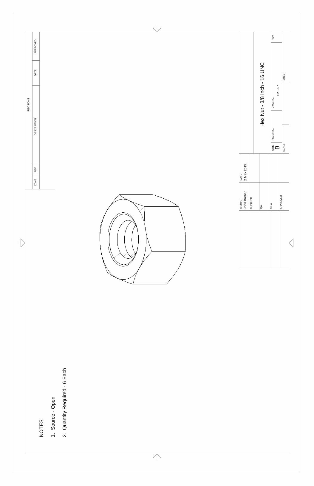
DR

AWN

QA

SCAL

E

BD

WG

NO

.M

FG

CH

ECKE

D

DES

CR

IPTI

ON

2 M

ay 2

015

DAT

E

DAT

E

SIZE

SK

-007

FSC

M N

O.

APPR

OVE

D

REV

ISIO

NS

REV

SHEE

T

REV

APPR

OVE

D

ZON

E

John

Bar

ber

Hex

Nut

- 3/

8 In

ch -

16 U

NC

NO

TES

1. S

ourc

e - O

pen

2. Q

uant

ity R

equi

red

- 6 E

ach

86

Appendix B - Complete Raw Data Table

Drop

Num

ber

Wed

ge

Angle

(Degrees)

Num

ber

of Top

Plates

Drop

Height

(Feet)

Weight

(Lbs)

Sand

Pe

netration

Dep

th(In

ches)

Actual Im

pulse

Magnitude

(G's)

Actual Im

pulse

Duration

(Millisecon

ds)

Impa

ct

Velocity

(Ft/Sec)

Pitch at

Impa

ct

(deg)

Roll at

Impa

ct

(deg)

Strain

Right

Vertical Strain Left

Vertical

Strain Right

Horizon

tal

Strain Left

Horizon

tal

145

13

104.0

6.0

9.9

83.5

13.6

2.2

0.3

19.0

10.0

7.0

7.0

245

13

100.2

4.0

6.7

122.5

13.4

‐1.1

1.8

<58.0

<56.0

345

13

100.2

4.5

6.6

117.5

13.6

‐5.0

‐0.7

<58.0

7.0

<54

451

310

0.2

4.5

6.3

133.0

13.5

‐1.4

‐2.3

<510

.0<5

<55

451

310

0.2

5.0

6.2

136.0

13.7

‐3.4

1.6

<57.0

<5<5

645

23

130.0

8.0

10.3

98.5

13.2

1.2

4.9

21.0

14.0

8.0

13.0

745

23

137.0

6.0

5.9

137.0

13.0

‐2.1

‐6.1

7.0

‐6.0

‐8

452

313

7.0

6.0

6.1

147.9

13.2

‐1.2

‐0.8

<5‐

<5‐

945

23

137.0

5.5

5.9

175.9

13.7

‐3.7

‐0.7

9.0

15.0

7.0

10.0

1045

23

137.0

6.0

5.8

149.9

13.1

2.4

3.2

8.0

11.0

<59.0

1145

33

159.0

9.0

9.5

112.5

13.6

‐1.8

‐5.9

19.0

30.0

9.0

16.0

1245

33

165.5

6.0

5.9

148.0

13.7

‐0.9

2.9

<529

.0<5

20.0

1345

33

165.5

6.5

5.7

189.5

13.6

‐2.0

1.3

<514

.0<5

<514

453

316

5.5

7.0

5.6

162.5

13.6

0.3

4.7

<520

.06.0

<515

453

316

5.5

7.0

5.5

162.5

13.6

0.5

6.1

<528

.07.0

18.0

1645

43

189.0

9.0

9.4

112.0

13.4

‐1.3

‐9.2

24.0

61.0

16.0

24.0

1745

43

194.2

7.0

5.5

163.0

13.7

‐1.6

6.1

11.0

35.0

7.0

14.0

1845

43

194.2

6.5

5.6

157.0

13.8

2.0

5.0

11.0

20.0

7.0

21.0

1945

43

194.2

7.5

5.5

151.5

13.7

‐0.2

1.1

8.0

13.0

7.0

<520

454

319

4.2

7.0

5.5

143.0

13.7

1.4

‐0.6

8.0

16.0

6.0

6.0

2145

53

218.0

9.5

8.6

116.0

13.1

‐1.0

‐3.1

18.0

35.0

23.0

21.0

2245

53

225.4

6.8

5.7

139.5

13.7

3.2

5.6

<520

.08.0

155.0

2345

53

225.4

7.0

5.6

120.0

13.7

3.1

5.6

13.0

25.0

10.0

15.0

2445

53

225.4

6.8

5.7

156.0

13.7

0.6

1.2

10.0

11.0

9.0

8.0

2545

53

225.4

7.0

5.5

151.0

13.7

2.8

6.4

13.0

40.0

9.0

39.0

2645

63

247.0

10.5

8.9

102.5

13.3

‐4.9

‐3.9

22.0

24.0

36.0

35.0

2745

63

251.7

7.0

5.4

144.5

13.6

‐1.5

7.7

44.0

86.0

11.0

25.0

2845

63

252.0

7.3

5.5

153.5

13.6

1.4

4.8

52.0

57.0

11.0

12.0

2945

63

252.0

7.8

5.3

139.0

13.7

‐0.7

2.4

44.0

35.0

7.0

<530

456

325

2.0

7.8

5.4

129.5

13.8

2.6

3.3

36.0

42.0

6.0

<531

457

327

7.0

11.5

8.1

119.0

13.6

‐2.9

‐6.0

38.0

25.0

52.0

62.0

3245

73

281.0

7.5

5.4

123.0

13.5

1.1

5.1

15.0

56.0

22.0

23.0

3345

73

281.0

7.8

5.2

159.5

13.7

1.4

2.3

23.0

47.0

13.0

24.0

3445

73

281.0

8.0

5.4

156.0

13.8

1.6

4.1

18.0

42.0

17.0

16.0

3545

73

281.0

8.0

5.2

163.0

13.7

1.7

5.5

18.0

44.0

14.0

21.0

3655

13

93.0

8.0

8.2

112.0

13.3

‐3.5

‐13.2‐

‐‐

‐37

552

312

2.0

7.5

9.2

105.0

13.2

‐0.1

‐9.8

33.0

13.0

‐12

.038

553

315

0.0

7.0

8.0

108.0

13.2

‐0.4

‐5.5

38.0

13.0

‐11

.039

554

318

0.0

7.0

7.7

119.0

13.1

‐3.3

‐5.1

‐‐

‐‐

4055

53

210.0

8.0

7.0

107.0

13.0

‐4.1

‐3.2

56.0

17.0

‐15

.0

Drop

Num

ber

Wed

ge

Angle

(Degrees)

Num

ber

of Top

Plates

Drop

Height

(Feet)

Weight

(Lbs)

Sand

Pe

netration

Dep

th(In

ches)

Actual Im

pulse

Magnitude

(G's)

Actual Im

pulse

Duration

(Millisecon

ds)

Impa

ct

Velocity

(Ft/Sec)

Pitch at

Impa

ct

(deg)

Roll at

Impa

ct

(deg)

Strain

Right


Vertical

Strain Right

Horizon

tal

Strain Left

Horizon

tal

4155

63

239.0

8.0

6.7

134.0

13.2

‐3.0

‐11.6

56.0

24.0

‐26

.042

557

326

8.0

7.5

8.4

105.5

13.2

‐0.9

‐1.7

55.0

24.0

‐28

.043

651

385

.04.0

9.8

81.0

13.1

1.0

3.4

7.0

5.0

6.0

6.0

4465

23

115.0

6.0

10.3

101.0

13.1

‐3.4

‐4.5

17.0

30.0

13.0

10.0

4565

33

144.0

5.0

9.5

88.5

13.1

‐1.5

‐5.1

23.0

28.0

4.0

14.0

4665

43

172.0

6.5

8.2

121.5

13.2

‐4.4

‐6.2

22.0

25.0

14.0

3.0

4765

53

201.0

6.5

9.2

105.0

13.2

‐2.1

‐2.2

48.0

62.0

10.0

7.0

4865

63

230.0

7.0

9.2

107.0

13.3

‐3.8

‐2.2

53.0

40.0

22.0

18.0

4965

73

259.0

8.5

8.6

108.0

13.3

‐3.0

‐4.6

66.0

75.0

17.0

31.0

5075

13

86.0

4.5

11.8

82.0

12.8

‐3.9

‐3.1

22.0

11.0

14.0

5.0

5175

23

111.0

3.5

10.4

88.0

13.4

‐‐

10.0

24.0

15.0

12.0

5275

33

140.0

5.0

9.9

92.0

13.4

‐0.9

3.0

25.0

40.0

17.0

17.0

5375

43

170.0

6.0

9.6

116.0

13.5

0.9

‐3.5

62.0

59.0

19.0

16.0

5475

53

198.0

6.0

9.3

101.0

13.5

‐‐

38.0

50.0

23.0

20.0

5575

63

228.0

5.5

9.0

98.0

13.6

‐0.6

2.8

70.0

54.0

15.0

23.0

5675

73

257.0

7.0

8.5

123.5

13.6

‐2.5

‐2.1

103.0

110.0

18.0

20.0

5745

15

104.0

6.3

13.5

80.5

17.3

1.4

3.5

21.0

17.0

10.0

10.0

5845

15

101.0

6.0

8.6

114.0

17.7

‐3.5

‐2.1

<5<5

<5<5

5945

15

101.0

6.0

8.3

153.0

17.7

‐2.9

1.4

<5<5

<59.0

6045

15

101.0

6.0

8.5

151.0

17.6

‐3.1

1.0

6.0

<5<5

7.0

6145

15

101.0

6.0

8.3

136.0

17.7

‐1.4

3.4

11.0

<5<5

<562

452

513

0.0

8.5

12.8

89.5

17.3

1.3

‐4.3

13.0

‐8.0

‐63

452

513

7.0

7.0

7.5

150.7

17.6

2.2

1.0

19.0

32.0

13.0

13.0

6445

25

137.0

7.0

7.5

159.0

17.7

0.9

4.0

15.0

29.0

9.0

15.0

6545

25

137.0

7.0

7.6

156.5

17.6

0.2

5.7

13.0

36.0

8.0

11.0

6645

25

137.0

7.0

7.6

152.0

17.6

‐1.8

2.8

19.0

26.0

10.0

17.0

6745

35

159.0

10.0

12.5

108.5

17.5

‐0.7

‐6.8

17.0

32.0

10.0

18.0

6845

35

165.5

7.3

7.5

158.5

17.6

‐2.3

5.5

9.0

12.0

6.0

17.0

6945

35

165.5

7.3

7.2

153.0

17.7

3.2

22.7

27.0

100.0

15.0

36.0

7045

35

165.5

7.3

7.3

151.5

17.6

3.4

10.1

17.0

52.0

11.0

21.0

7145

35

165.5

7.5

7.6

153.5

17.6

2.3

5.6

12.0

45.0

9.0

14.0

7245

45

189.0

10.0

12.4

89.0

17.7

‐3.7

‐11.8

27.0

74.0

17.0

23.0

7345

45

194.7

8.0

7.4

155.0

17.6

1.1

4.0

9.0

23.0

8.0

27.0

7445

45

194.7

8.3

7.2

157.5

17.7

‐1.0

4.5

14.0

35.0

11.0

18.0

7545

45

194.7

8.0

7.5

146.5

17.6

1.3

5.0

17.0

42.0

14.0

19.0

7645

45

194.7

8.0

7.2

158.0

17.7

2.3

6.7

18.0

38.0

12.0

6.0

7745

55

218.0

10.5

11.3

128.5

17.4

‐1.8

‐5.9

24.0

65.0

27.0

24.0

7845

55

224.5

8.5

6.7

157.0

17.6

2.5

12.2

41.0

121.0

18.0

43.0

7945

55

224.5

7.8

7.5

139.5

17.6

1.2

0.7

9.0

10.0

10.0

11.0

8045

55

224.5

7.8

7.5

195.5

17.6

1.0

3.7

12.0

24.0

13.0

13.0

Drop

Num

ber

Wed

ge

Angle

(Degrees)

Num

ber

of Top

Plates

Drop

Height

(Feet)

Weight

(Lbs)

Sand

Pe

netration

Dep

th(In

ches)

Actual Im

pulse

Magnitude

(G's)

Actual Im

pulse

Duration

(Millisecon

ds)

Impa

ct

Velocity

(Ft/Sec)

Pitch at

Impa

ct

(deg)

Roll at

Impa

ct

(deg)

Strain

Right


Vertical

Strain Right

Horizon

tal

Strain Left

Horizon

tal

8145

55

224.5

7.8

7.6

147.0

17.6

‐1.3

1.3

9.0

20.0

14.0

12.0

8245

65

247.0

11.5

10.8

113.0

17.4

‐5.3

‐8.3

26.0

26.0

37.0

40.0

8345

65

252.0

8.0

7.3

160.0

17.6

0.2

8.5

57.0

110.0

11.0

21.0

8445

65

252.0

8.5

7.1

151.0

17.5

1.8

8.0

49.0

84.0

13.0

33.0

8545

65

252.0

8.5

7.4

145.0

17.6

1.0

2.7

63.0

75.0

12.0

12.0

8645

65

252.0

8.8

7.2

162.0

17.7

1.7

7.2

51.0

75.0

17.0

8.0

8745

75

277.0

12.0

9.9

125.5

17.7

‐2.6

‐12.4

37.0

99.0

51.0

38.0

8845

75

281.0

9.5

7.0

148.0

17.6

2.1

13.1

40.0

118.0

25.0

41.0

8945

75

281.0

9.5

6.3

157.0

17.6

2.1

19.0

64.0

184.0

28.0

64.0

9045

75

282.0

10.0

6.2

151.0

17.4

‐2.9

36.7

80.0

237.0

34.0

77.0

9145

75

282.0

9.5

7.3

142.0

17.4

5.4

10.0

29.0

78.0

30.0

37.0

9255

15

93.0

7.5

14.3

108.0

17.4

‐6.1

‐17.9‐

‐‐

‐93

552

512

2.0

7.5

13.3

92.0

17.4

‐4.2

‐4.8

‐‐

‐‐

9455

35

150.0

8.5

12.2

130.5

17.4

‐0.8

‐15.8

34.0

14.0

‐13

.095

554

518

0.0

8.5

11.3

146.5

17.4

‐4.7

‐14.3

67.0

26.0

‐22

.096

555

521

0.0

9.0

11.1

121.5

17.3

‐2.3

‐8.8

42.0

26.0

‐20

.097

556

523

9.0

9.5

10.7

136.0

17.4

‐2.2

‐12.8

71.0

34.0

‐40

.098

557

526

8.0

9.0

10.9

125.0

17.5

‐2.4

‐10.3

72.0

41.0

‐32

.099

651

585

.05.0

15.4

88.5

17.4

‐1.7

‐11.1

8.0

5.0

16.0

11.0

100

652

511

5.0

6.0

14.9

114.0

17.4

‐1.7

‐9.3

23.0

39.0

11.0

19.0

101

653

514

4.0

7.0

14.4

111.5

17.3

‐3.1

‐7.2

54.0

56.0

16.0

24.0

102

654

517

2.0

7.5

13.2

127.5

17.4

‐1.5

‐14.8

60.0

52.0

16.0

15.0

103

655

520

1.0

8.0

12.9

127.5

17.5

‐2.5

‐14.1

93.0

82.0

16.0

20.0

104

656

523

0.0

8.0

12.6

101.0

17.4

2.7

2.0

46.0

63.0

18.0

32.0

105

657

525

9.0

8.5

11.3

121.0

17.3

0.8

6.6

46.0

102.0

15.0

21.0

106

751

586

.05.0

16.1

108.5

17.2

2.8

14.7

20.0

27.0

23.0

14.0

107

752

511

1.0

4.5

15.0

87.5

17.6

1.4

0.4

24.0

34.0

20.0

15.0

108

753

514

0.0

6.0

13.8

96.5

17.7

‐‐

53.0

56.0

15.0

14.0

109

754

517

0.0

7.0

13.7

121.0

17.7

‐1.0

‐6.5

76.0

56.0

26.0

15.0

110

755

519

8.0

6.5

12.5

116.0

17.7

‐‐

72.0

69.0

13.0

23.0

111

756

522

8.0

6.5

12.3

117.0

17.6

0.1

‐0.9

89.0

72.0

28.0

22.0

112

757

525

7.0

8.0

13.0

123.5

17.7

‐2.0

‐3.2

97.0

118.0

27.0

38.0

113

451

710

4.0

8.0

16.7

83.5

20.9

2.2

3.3

17.0

19.0

18.0

20.0

114

451

710

1.0

6.5

10.3

132.0

20.8

‐1.8

9.3

15.0

6.0

6.0

<511

545

17

101.0

6.5

10.0

136.0

21.0

‐1.2

13.7

27.0

12.0

11.0

<511

645

17

101.0

6.5

10.0

134.5

20.9

‐1.1

13.5

28.0

13.0

13.0

7.0

117

451

710

1.0

6.5

9.8

138.0

20.8

‐1.3

11.8

27.0

<59.0

<511

845

27

130.0

9.5

16.6

86.0

20.8

5.6

‐0.7

35.0

45.0

17.0

21.0

119

452

713

7.0

7.8

9.1

148.5

20.8

3.2

‐0.3

26.0

32.0

17.0

18.0

120

452

713

7.0

7.8

9.3

145.5

20.7

1.9

‐0.9

19.0

33.0

12.0

16.0

Drop

Num

ber

Wed

ge

Angle

(Degrees)

Num

ber

of Top

Plates

Drop

Height

(Feet)

Weight

(Lbs)

Sand

Pe

netration

Dep

th(In

ches)

Actual Im

pulse

Magnitude

(G's)

Actual Im

pulse

Duration

(Millisecon

ds)

Impa

ct

Velocity

(Ft/Sec)

Pitch at

Impa

ct

(deg)

Roll at

Impa

ct

(deg)

Strain

Right


Vertical

Strain Right

Horizon

tal

Strain Left

Horizon

tal

121

452

713

7.0

7.8

9.3

143.0

20.8

2.4

‐1.1

22.0

29.0

13.0

17.0

122

452

713

7.0

8.0

9.4

123.5

20.8

‐2.2

1.6

26.0

35.0

16.0

23.0

123

453

715

9.0

10.5

15.4

81.0

20.8

‐2.1

‐9.6

33.0

63.0

18.0

28.0

124

453

716

5.5

8.5

9.1

155.5

20.9

0.7

8.8

16.0

50.0

14.0

9.0

125

453

716

5.5

8.0

8.6

154.5

20.9

6.8

18.4

31.0

93.0

14.0

31.0

126

453

716

5.5

8.3

8.8

159.0

20.9

1.5

3.9

14.0

44.0

11.0

11.0

127

454

718

9.0

11.5

15.4

125.0

20.7

‐3.1

‐9.8

31.0

71.0

16.0

21.0

128

454

719

5.2

9.0

8.4

161.0

20.9

4.6

19.3

32.0

76.0

22.0

40.0

129

454

719

5.2

9.0

8.9

157.0

20.8

2.8

10.9

21.0

69.0

8.0

32.0

130

454

719

5.2

8.8

9.1

158.0

21.0

1.9

3.1

18.0

43.0

15.0

13.0

131

454

719

5.2

8.8

8.2

155.0

21.0

0.4

1.6

14.0

33.0

13.0

14.0

132

455

721

8.0

11.5

14.4

123.5

20.7

‐6.8

‐8.3

38.0

91.0

49.0

49.0

133

455

722

5.1

9.0

8.8

142.0

20.9

‐1.3

6.8

21.0

53.0

15.0

31.0

134

455

722

5.1

8.5

9.1

141.5

20.9

1.2

5.8

17.0

50.0

25.0

30.0

135

455

722

5.1

9.0

9.0

131.5

20.8

‐1.2

6.1

32.0

84.0

20.0

45.0

136

455

722

5.1

8.8

9.0

157.0

21.0

1.0

4.4

16.0

50.0

23.0

33.0

137

456

724

7.0

12.0

13.4

123.5

20.8

‐4.6

‐12.2

21.0

51.0

58.0

68.0

138

456

725

2.5

9.5

8.9

158.0

21.0

2.0

4.4

60.0

98.0

14.0

14.0

139

456

725

2.5

9.5

8.9

169.5

21.0

3.9

4.4

58.0

97.0

11.0

26.0

140

456

725

2.5

9.5

8.7

150.5

21.0

1.2

9.9

51.0

121.0

19.0

32.0

141

456

725

2.5

9.8

8.9

150.5

21.0

1.4

11.7

78.0

142.0

17.0

23.0

142

457

727

7.0

13.5

13.0

135.0

20.8

‐2.9

‐19.8

41.0

91.0

80.0

78.0

143

457

728

2.0

10.0

7.4

150.0

20.9

4.4

28.2

76.0

201.0

32.0

59.0

144

457

728

2.0

10.0

7.4

156.5

20.9

6.3

34.8

94.0

240.0

41.0

65.0

145

457

728

2.0

10.0

8.6

153.5

21.0

3.6

21.7

60.0

168.0

50.0

39.0

146

457

728

1.0

10.0

7.9

157.5

21.0

1.5

7.8

42.0

127.0

49.0

47.0

147

551

793

.07.0

17.8

96.5

20.7

‐5.9

‐25.0

35.0

17.0

‐7.0

148

552

712

2.0

8.5

17.1

109.0

20.6

‐4.7

‐7.5

‐‐

‐‐

149

553

715

0.0

9.0

16.8

126.0

20.6

‐1.8

‐17.4

44.0

23.0

‐24

.015

055

47

180.0

9.0

15.1

127.0

20.8

‐7.7

‐19.4

58.0

14.0

‐36

.015

155

57

210.0

9.5

15.0

121.5

20.7

‐1.2

‐6.6

59.0

36.0

‐34

.015

255

67

239.0

10.0

14.1

133.5

20.8

‐2.8

‐15.5

89.0

52.0

‐60

.015

355

77

268.0

10.0

14.4

130.0

21.0

‐3.7

‐19.0

101.0

56.0

‐57

.015

465

17

85.0

6.0

18.9

87.0

20.5

‐4.4

‐17.7

20.0

18.0

9.0

16.0

155

652

711

5.0

7.0

18.8

116.5

20.6

‐1.6

‐9.8

52.0

77.0

29.0

28.0

156

653

714

4.0

7.5

18.4

95.0

20.7

‐1.9

‐2.1

68.0

89.0

37.0

28.0

157

654

717

2.0

8.5

16.9

124.0

20.7

‐2.0

‐12.5

65.0

83.0

26.0

36.0

158

655

720

1.0

9.0

16.5

155.0

20.7

‐4.4

‐9.3

124.0

121.0

27.0

22.0

159

656

723

0.0

9.5

15.8

122.0

20.5

‐5.5

‐13.9

142.0

67.0

58.0

28.0

160

657

725

9.0

9.0

15.9

109.5

20.7

‐3.8

‐4.1

131.0

149.0

34.0

21.0

Drop

Num

ber

Wed

ge

Angle

(Degrees)

Num

ber

of Top

Plates

Drop

Height

(Feet)

Weight

(Lbs)

Sand

Pe

netration

Dep

th(In

ches)

Actual Im

pulse

Magnitude

(G's)

Actual Im

pulse

Duration

(Millisecon

ds)

Impa

ct

Velocity

(Ft/Sec)

Pitch at

Impa

ct

(deg)

Roll at

Impa

ct

(deg)

Strain

Right


Vertical

Strain Right

Horizon

tal

Strain Left

Horizon

tal

161

751

786

.05.5

20.5

86.0

20.5

‐3.9

‐10.8

45.0

17.0

12.0

12.0

162

752

711

1.0

5.5

18.3

94.0

20.8

‐0.9

‐0.6

37.0

47.0

18.0

10.0

163

753

714

0.0

6.0

17.8

96.5

20.9

‐1.6

‐0.7

62.0

92.0

26.0

24.0

164

754

717

0.0

7.0

16.8

123.0

20.9

‐0.5

‐6.0

103.0

94.0

38.0

13.0

165

755

719

8.0

7.5

16.5

125.5

20.9

‐1.3

‐7.1

129.0

106.0

40.0

44.0

166

756

722

8.0

7.0

16.4

116.5

21.0

‐‐

139.0

127.0

31.0

43.0

167

757

725

7.0

8.5

16.9

139.0

21.0

‐1.0

‐19

7.0

154.0

29.0

24.0

168

451

910

4.0

8.5

19.8

88.5

24.1

0.2

‐20.5

28.0

60.0

3.0

17.0

169

451

910

2.5

7.0

11.5

136.3

23.1

‐0.8

2.1

98.0

‐37

.0‐

170

451

910

2.5

7.0

11.2

132.2

23.1

‐0.5

‐5.2

91.0

‐35

.0‐

171

451

910

2.5

7.5

11.5

120.1

23.1

‐0.5

4.1

88.0

‐30

.0‐

172

451

910

2.5

7.0

11.1

137.4

23.8

0.3

1.9

98.0

‐34

.0‐

173

452

913

0.0

10.5

19.0

108.0

24.0

‐5.1

‐8.3

50.0

71.0

27.0

31.0

174

452

913

7.0

7.5

11.5

134.5

23.7

0.1

4.7

25.0

31.0

13.0

15.0

175

452

913

7.0

7.8

11.0

147.0

23.8

2.2

3.9

25.0

35.0

18.0

28.0

176

452

913

7.0

8.0

11.2

138.5

23.7

‐0.9

0.2

17.0

31.0

19.0

24.0

177

452

913

7.0

8.8

11.0

146.5

23.8

0.9

5.1

27.0

41.0

19.0

15.0

178

453

915

9.0

11.5

18.3

81.0

24.0

‐1.9

‐6.6

28.0

54.0

17.0

23.0

179

453

916

5.5

9.0

10.4

149.0

23.9

5.2

17.9

29.0

91.0

14.0

28.0

180

453

916

5.5

9.0

10.4

156.5

23.7

1.7

8.0

21.0

63.0

11.0

19.0

181

453

916

5.5

9.5

10.4

150.0

23.8

6.1

14.6

30.0

60.0

13.0

31.0

182

453

916

5.5

9.5

11.0

152.5

24.0

3.6

6.8

17.0

27.0

13.0

29.0

183

454

918

9.0

11.8

17.6

104.0

23.7

2.3

‐4.0

33.0

57.0

58.0

37.0

184

454

919

6.0

8.5

10.6

153.0

23.7

5.2

13.8

24.0

70.0

17.0

32.0

185

454

919

6.0

9.0

10.5

150.5

24.0

4.2

7.2

19.0

51.0

19.0

201.0

186

454

919

6.0

9.0

10.2

154.5

23.8

5.8

11.8

24.0

62.0

13.0

420.0

187

454

919

8.3

9.0

10.4

150.0

23.8

5.8

16.2

29.0

85.0

21.0

55.0

188

455

921

8.0

12.8

17.0

130.0

24.0

‐1.7

‐12.0

41.0

104.0

80.0

77.0

189

455

922

5.8

9.8

10.6

146.0

23.8

‐0.2

6.8

19.0

61.0

32.0

110.0

190

455

922

5.8

9.5

10.5

148.5

23.7

2.1

5.7

20.0

47.0

28.0

17.0

191

455

922

5.8

9.3

10.7

133.5

23.8

2.1

0.7

14.0

21.0

31.0

18.0

192

455

922

5.7

9.8

10.8

154.0

23.8

0.9

6.6

29.0

97.0

27.0

40.0

193

456

924

7.0

13.5

16.3

109.0

24.0

‐8.5

‐20.7

38.0

104.0

110.0

171.0

194

456

925

3.0

10.0

9.6

153.0

23.7

2.4

13.8

94.0

130.0

16.0

26.0

195

456

925

3.0

10.0

10.9

146.5

23.8

1.0

8.6

112.0

79.0

32.0

120.0

196

456

925

3.0

10.0

10.4

151.0

23.8

0.8

13.0

106.0

67.0

29.0

280.0

197

456

925

3.0

10.0

10.3

148.5

23.8

0.2

15.5

115.0

173.0

22.0

173.0

198

457

927

7.0

14.8

15.1

139.5

24.0

‐5.3

‐23.2

36.0

153.0

118.0

159.0

199

457

928

1.0

10.0

9.5

151.5

23.7

3.1

31.9

84.0

210.0

42.0

65.0

200

457

928

1.0

10.0

10.0

156.5

23.8

2.1

23.9

64.0

180.0

58.0

49.0

Drop

Num

ber

Wed

ge

Angle

(Degrees)

Num

ber

of Top

Plates

Drop

Height

(Feet)

Weight

(Lbs)

Sand

Pe

netration

Dep

th(In

ches)

Actual Im

pulse

Magnitude

(G's)

Actual Im

pulse

Duration

(Millisecon

ds)

Impa

ct

Velocity

(Ft/Sec)

Pitch at

Impa

ct

(deg)

Roll at

Impa

ct

(deg)

Strain

Right


Vertical

Strain Right

Horizon

tal

Strain Left

Horizon

tal

201

457

928

1.0

10.0

9.6

157.0

23.8

1.6

12.7

55.0

161.0

59.0

50.0

202

457

928

1.0

10.0

10.3

154.5

23.6

2.4

23.1

85.0

204.0

64.0

176.0

203

551

993

.08.0

22.0

99.0

23.9

‐3.0

‐25.4

36.0

22.0

‐24

.020

455

29

122.0

9.0

20.2

117.5

23.9

‐1.4

‐12.6

47.0

23.0

‐31

.020

555

39

150.0

9.5

19.4

135.5

23.9

‐3.3

‐18.4

46.0

31.0

‐37

.020

655

49

180.0

9.5

19.4

104.5

23.8

0.3

6.4

60.0

69.0

‐70

.020

755

59

210.0

10.5

17.9

121.0

23.9

‐4.2

‐14.4

70.0

58.0

‐58

.020

855

69

239.0

11.5

17.7

131.0

23.9

‐2.3

‐12.2

94.0

91.0

‐88

.020

955

79

268.0

10.5

17.1

118.0

24.1

‐5.1

‐20.5

168.0

105.0‐

165.0

210

651

985

.06.5

23.3

81.0

23.8

‐3.2

‐9.4

‐‐

‐‐

211

652

911

5.0

7.5

22.3

61.0

23.8

‐2.1

‐11.7

83.0

93.0

22.0

23.0

212

653

914

4.0

8.5

21.5

110.5

23.8

‐3.5

‐8.2

138.0

134.0

70.0

46.0

213

654

917

2.0

9.0

19.7

130.5

23.8

‐4.9

14.6

159.0

102.0

55.0

30.0

214

655

920

1.0

9.5

20.2

140.5

23.9

‐3.5

‐11.5

279.0

186.0

69.0

31.0

215

656

923

0.0

9.5

19.2

117.0

23.8

‐2.3

‐5.7

202.0

148.0

64.0

55.0

216

657

925

9.0

9.5

19.3

91.5

24.0

‐5.4

0.0

198.0

240.0

26.0

69.0

217

751

986

.06.0

23.4

77.5

23.7

‐2.8

‐16.7

47.0

21.0

16.0

4.0

218

752

911

1.0

6.0

21.5

93.5

24.1

1.5

4.9

57.0

84.0

23.0

52.0

219

753

914

0.0

7.0

21.4

97.5

24.2

‐1.7

‐1.0

95.0

113.0

58.0

29.0

220

754

917

0.0

8.0

20.4

119.0

24.2

‐‐

151.0

158.0

47.0

19.0

221

755

919

8.0

8.0

20.5

129.5

24.3

‐‐

178.0

157.0

60.0

37.0

222

756

922

8.0

8.0

20.1

122.0

24.3

‐‐

140.0

185.0

32.0

30.0

223

757

925

7.0

8.5

19.9

139.5

24.2

‐4.4

‐5.4

268.0

239.0

29.0

56.0

93

VITA

John D. Barber

C/O

Batten College of Engineering and Technology

1105 Engineering Systems Building

Norfolk, VA 23529

Cell Phone: (757) 617-1546, E-mail: [email protected]

Education: University of Evansville, Mechanical Engineering, B.S., Jun 1985

Old Dominion University, Mechanical Engineering, M.S., Dec. 2016

General Experience:

2007 – Present Naval Surface Warfare Center, Carderock Division, Mechanical Engineer

2007 - 2007 Booz Allen Hamilton, Associate

2006 - 2007 Scientific Research Corporation, Senior Analyst

2000 - 2006 Naval Special Warfare Development Group, Mechanical Engineer

1985 - 2000 Naval Surface Warfare Center, Crane Division, Mechanical Engineer

Experience Summary:

Extensive experience in test and evaluation, test program planning and execution, test and

evaluation logistics support, test fixture design, demolition application software design and

support. Test and evaluation experience includes, small arms, small arms ammunition,

shoulder fired anti-tank weapons, hand emplaced demolition and small combatant craft.

parametric investigation of a laboratory drop test to

Documents