JO

© R-1693-1-PA&E February 1976

./-*'

1_ ( / y - -f

/

■a tti** .

Parametric Equations for Estimating Aircraft Airframe Costs

Joseph P. Large, Harry G. Campbell and David Cates

A

A Report prepared for /~w»

ASSISTANT SECRETARY OF DEFENSEllÜiJb'cjbJ U'id^ (PROGRAM ANALYSIS AND EVALUATION) A-

Rand SANTA MONICA < V 4WH,

,v...;;ed

·•·

THIS DOCUMENT IS BEST QUALITY AVAILABLE. THE COPY

FURNISHED TO DTIC CONTAINED

A SIGNIFICANT NUMBER OF

PAGES WHICH DO NOT

REPRODUCE LEGIBLYo

I ■

The research described in this Report was sponsored by the Office of the Assistant Secretary of Defense (Program Analysis and Evai.iation) under Contract DAHC 15 C 0220. Reports of The Rand Corporation do not necessarily reflect the opinions or policies of the sponsors of Rand research.

___________ __________

„m .„I, ■- ,.,■■■-,AJI

R-1693-1-PA&E February 1976

Parametric Equations for Estimating Aircraft Airframe Costs

Joseph P. Large, Harry G. Campbell and David Cates

A Report prepared for

ASSISTANT SECRETARY OF DEFENSE

(PROGRAM ANALYSIS AND EVALUATION)

i i

Rand SANIA MONICA. CA. 4040b

APPROVED FOR PUBLIC RELEASE; DISTRIBUTION UNLIMITED

riii i n im Tin IN rnn --iiiiittifinaaii mat«! r«t>—

BMae ,— -a-wfc

-iii-

PREFACE

***** 14? '4"

^ %c Afcj. _

'■*&* ^o

This study was sponsored by the Office of the Assistant Secretary

of Defense (Program Analysis and Evaluation) as part of a research pro-

gram focused on improved methods of estimating the development, procure-

ment, and operating costs of new weapon systems. The purpose of the

study was to derive equations for estimating the acquisition cost of

aircraft airframes. Such equations are intended primarily for use in

long-range planning, not for contract negotiation or financial manage-

ment.

This report was first distributed in May 1975. In the present

printing, dated February 1976, the author has supplied supplementary

material (Appendix C) illustrating how equations that appear to be com-

parable on the basis of statistical measurements can give widely differ-

ent estimates of cost. The repoit should be useful to persons concerned

with the selection, procurement, and production of military aircraft.

i

na^kaMH mm mmm -'-—-*"-■—"-—^*—>"

- - ■ '

«*&*. , ,«,ft

-V-

SUMMARY

^ ^ *4

%.

Studies pertaining to the selection and acquisition of military

aircraft generally begin with little more than a statement of the

anticipated weight and the desired performance of a proposed aircraft.

Even at that point, however, cost is an important consideration, and

cost-estimating techniques must be devised that require only the avail-

able information, i.e., estimates of a limited number of physical and

performance characteristics. This report presents generalized equa-

tions for estimating development and production costs of aircraft air-

frames on the basis of such characteristics as aircraft weight and

speed. It provides separate equations for the following cost elements:

engineering, tooling, nonrecurring manufacturing labor, recurring manu-

facturing labor, nonrecurring manufacturing material, recurring manu-

facturing material, flight-test operations, and quality control. It

also provides equations for estimating total program cost and prototype

development cost.

The estimating relationships are expressed in the form of expo-

nential equations derived by multiple-regression techniques. Costs or

man-hours are related to aircraft characteristics and quantity. In

earlier Rand work. ' it was found that the characteristics that best

explain variations in cost among airframes are airframe unit weight

and maximum speed. A determined effort was made in the present study

to find additional characteristics that would make an estimating model

more flexible and hence better able to deal with characteristics pecu-

liar to individual aircraft. That effort was not productive. The

variations in cost that are not explained by weight and speed are not

explained by any other objective parameters tested.

The equations presented here were derived from cost data on 25

military aircraft with first-flight dates from 1953 to 1970. (The

Levenson, G. S., and S. M. Barro, Cost-Ectimatinq Relationships for Aircraft Airframes, The Rand Corporation, RM-4845-PR, February 1966.

2

Levenson, G. S., et al., Cost-Estimating Relationships for Air- craft Airframes, The Rand Corporation, R-761-PR, December 1971.

..-.,.—,„... .—.....—.^,.„ .. : __„ ...— .■-._ ..:,.. . mHMMI

M~ 3L S^MÜfite'

-VI-

earlier work included aircraft developed as far back as 1946.) The

aircraft in the sample have airframe unit weights ranging from 5.000

to 279,000 lb and maximum speeds ranging from 300 to better than

1300 kn. Cost data were obtained directly from the airframe contrac-

tors whose aircraft appear in the sample and from standard Department

of Defense references such as the Cost Information Report (now the

Contractor Cost Data Reporting System).

The report explains the derivation of each of the estimating equa-

tions and describes the treatment of the data, the fitting of regres-

sion equationsv and the selection of preferred equations. Other

equations with additional explanatory variables <re included where the

statistical basis for choosing one equation over another is not strong.

A detailed numerical example is included which applies the preferred

equations and compares the results to those obtained using several

sets of alternative equations.

until rin'n -iin ■ nr-frtof,mMmimimtimmmim&u^m I il1r.liln1rr.Mr».Im- IXM—«M^«M^^ kattHü

States* "l&HJF**'-^

w-*i

-vii-

ACKNOWLEDGMENTS

The authors wish to express their appreciation for the coopera-

tion of the following major airframe companies: Boeing Aerospace

Company, Fairchild Republic Company, General Dynamics Corporation,

Grumman Aerospace Corporation, LTV Aerospace Corporation, Lockheed-

California Company, Lockheed-Georgia Company, McDonnell-Douglas Cor-

poration, Northrop Corporation, and Rockwell-International Corporation.

Their willingness to provide data made the analyses described here

possible. Within Rand technical assistance on engineering matters was

provided by G. K. Smith and T. F. Kirkwood. Smith also acted as tech-

nical reviewer along with B. D. Bradley and D. Dreyfuss, and their

comments were particularly helpful. H. E. Boren, Jr., K. Hoffmayer,

and F. Kontrovich assisted with data preparation.

.. .,.., ._^, ■II— —.»—~~.--.~~...... . . __^_

aLs ■•.^gi»-^ ; -*r-, IIM uy i—1 ; —SU^^^M,Ji ': ■ •

-ix-

CONTENTS

P-^Ci »**> p47* s^c iVby

'■füjSD

PREFACE iii

SUMMARY v

ACKNOWLEDGMENTS vii

Section I. INTRODUCTION 1

II. RESEARCH PROCEDURE 5 Data Acquisition and Review 5 Analytical Techniques 16

ill. ENGINEERING 18

IV. TOOLING 23

V. MANUFACTURING LABOR 27

VI. MANUFACTURING MATERIALS 31

VII. FLIGHT TEST 36

VIII. QUALITY CONTROL 38

IX. TOTAL COST 40

X. OTHER AVENUES EXPLORED 44 Judgment 44 Groupings 46

XI. PROTOTYPE AIRCRAFT 49

XII. CONCLUSIONS 53

Appendix A. AN ILLUSTRATIVE PKOBLEM 55 B. REGRESSION EQUATIONS AND STATISTICS 63 C. USING ESTIMATING EQUATIONS 113

■ --* M.->.M-|- ■irmnnirr 7riirn mmmmmm*tmm&mmt*mMMmiifm: -"tm

fic -k. I l'.ftiv.* «kij "■if;isv3WSR»-' ■..,,?.;.

■1-

I. INTRODUCTION

For many years estimates of aircraft airframe cost were based

mainly on weight. The ARCO factor, for example (which took its name

from the World War II Aircraft Resources Control Office), stipulated

that manufacturing hours per pound of airframe could be estimated

solely on the basis of airframe weight and production quantity. For

a given quantity all aircraft were estimated from the same curve.

In the years since then estimators have been searching for other

aircraft characteristics that (1) will, in combination with weight,

provide consistently accurate estimates, (2) are logically related to

cost, and (3) can easily be determined prior to actual design and de-

velopment. The third requirement has led to use of characteristics

such as speed, wetted area, and aspect ratio, rather than those that

require more detailed knowledge such as number of engineering drawings

or number of parts. A model published by Rand in 1966 showed that

weight and speed were the only two explanatory variables that met the

three criteria cited. The model produced estimates that were found

useful both by government and by industry, but the feeling lingered

that it should be possible to achieve greater accuracy by including

new and different variables.

Other companies, looking at ostensibly the same data, had developed

models using additional variables. Planning Research Corporation, for

example, found time to be an important variable for material costs.

Consequently, it was felt that a revised model could perhaps be more

flexible, more responsive to program variations such as type of de-

velopment program and development schedule. Also, after several years

the addition of new aircraft to the U.S. inventory meant that the sam-

ple size could be increased and the enlarged sample would be more

representative of aircraft likely to be developed in the future.

Levenson, G. S., and S. M Barro, Cost-Estimatinj Relationships for Air-craft Airframes, The Rano Corporation, PM-4845-PR, February 1966.

2 Method:! cf Estimating Fixed-Wing Airframe Costs, Vol. 1 (Revised),

PRC-547A, April 1967.

-i- _an

-2-

A revised model was published by Rand in 1971. Several aircraft

were added to the data base, a method for distinguishing between proto-

type and full development programs was added, and the procedures followed

in developing the model were less judgmental. Users pointed out almost

immediately, however, that the model suffered from what were believed to

be shortcomings in the earlier version: (1) the only two major explan-

atory variables were weight and speed; (2) all aircraft were lumped

together rather than treated as classes (e.g., fighters, bombers, etc.);

and (3) no provision was made for taking into account changes in air-

frame structural materials and manufacturing methods. Consequently,

when information on several new aircraft became available and it seemed

desirable to update the data base, OSD (PA&E)M agreed to sponsor a re-

search effort to produce a new estimating model and in the process deal

explicitly with the questions raised earlier.

The study plan called for:

1. Review of airframe data in the Rand files to ensure accuracy

and consistency of definition and acquisition data on new

aircraft.

2. Consideration of additional explanatory variables that would

make the model better able to deal with characteristics

peculiar to individual aircraft, e.g., variable-geometry

wing, oversize fuselage.

3. Examination of the cost impact of major changes in manufac-

turing technology over time and of the use of different

structural materials.

Reviewing and expanding the data base turned out to be more of a

job than was anticipated. Data had been collected over a period of

years from a variety of sources, and to ensure internal consistency it

was necessary to obtain additional cost details from airfrsme contractors.

"Levenson, G. S., et al., Coat-Estimathuj Itelationshipa for Air- craj't Airframcs, The Rand Corporation, R-761-PR, December 1971.

The Office of the Assistant Secretary of Defense ("rogram Analysis and Evaluation).

■■

Our goal was to obtain total contract cost for every contract of in-

terest (i.e., out through the first few huudied aircraft) for over

30 military aircraft. In the time available it was not possible to

resolve all the questions concerning data, but we believe our data

sample is far more complete, comparable, and accurate than those used

in previous analyses.

Our search for other explanatory variables that would improve the

accuracy of estimates was less fruitful than we had hoped. The varia-

tions in cost that are not explained by weight and speed are not ex-

plained by any other objective indexes that we could find. For several

of the cost elements, use of a dummy variable to distinguish cargo

aircraft from other types proved beneficial. None of the other 20 or

so variables considered, however, satisfied the criteria for inclusion.

It was necessary to examine the cost implications of major changes

in airframe manufacturing technology and structural materials because

the data sample consists largely of aluminum aircraft. The shift to

other materials such as steel, titanium, and composites raises a ques-

tion about the value of equations derived from that sample for estimat-

ing the cost of future aircraft. Titanium is much more expensive than

aluminuu. and is more difficult to fabricate. The fasteners used to

join titanium structural parts are many times more expensive on a per-

unit basis than those customarily used in airframe assembly. On the

other hand, adoption of a "unitized design concept" by some producers

has reduced the number of parts and fasteners required. Thus the in-

crease in fabrication man-hours may be offset by a decrease in assembly

man-hours, and the shift would presumably result in a flattening of the

cost-quantity curve. Statistical analysis does suggest a trend toward

higher material costs and reduced manufacturing man-hours, and we dis-

cuss some of the qualitative considerations involved later in this

report.

The estimating model developed is similar to previous Rand models

in that it allows estimates to be made of individual cost elements

(except in the case of prototype programs). An additional feature is

that it a.lows estimates to be made of total program cost with no

separation into cost elements. Several contractors suggested that more

iitMmin ■MI.IM i

-4-

ac;urate estimates could be achieved by estimating at the total pro-

gram level, and a report on aircraft estimating prepared for the U.S.

Navy makes a similar recommendation.1 Our conclusion is that the

results obtained from the two methods are comparable; we cannot say

that either method gives consistently better estimates.

Noah, J. W., et al., Estimating Aircraft Acquisition Costs by Parametric Methods, J. Watson Noah Associates, Inc., FR-103-liSN (abridged), September 1973.

i ■ iffi-'^'' '■ ii--I"I ."•—■" -^'f-i■■■-■■ ■-- '-": ■'—■*--'--WifriiiVi iiirTirf*'" * ^ "'" *'""_

-5-

II. RESEARCH PROCEDURE

DATA ACQUISITION AND REVIEW

The cost data used in this study were obtained from both govern-

ment and industry, and within the time available every effort was made

to ensure that the data were complete and comparable. Our goal was to

obtain total contract cost for every contract of interest (i.e., out

through the first few hundred aircraft) and to break that cost down

into all the elements shown on the worksheet in Fig. 1. That amount

of detail was not available for some of ehe older aircraft in the

sample, but with the generous cooperation of major airframe contrac-

tors enough data were obtained to make sure that most costs are in-

cluded and properly classified. The sample consists of the following

aircraft:

A-3 C-133 F-86D A-4 KG-135 F-89 A-5 C-141 F-100 A-6 F3D F-102 A-7 F-3 F-104 B-47 F-6 F-105 B-52 r-4 F-106 B-58 F-14 F-lll RB-66 F-84A T-38 C-5 F--86A T-39 C-130

Before the final analyses were made, all aircraft with first flight

dates prior to 1952 (i.e., the B-47, F3D, F-84A, F-H6A, F-86D, r.nd F-89)

were deleted from the sample, partially because of problems with the

data and partially because development and production experience on air-

craft that old does not appear to be a reliable guide to the future.

A basic question when dealing with data recorded by so many dif-

ferent contractors over so many years is whether to use actual costs

or normalized costs. Actual costs may reflect problems that are irrel-

evant to the task of developing and producing an aircraft. A severe

labor shortage, for example, may caus;e a contractor to hire unqualified

- -: - — -■- —- -—naMM(Mfi,Lifiiiri-—inniTüMi "imiimi rmtiiiir i. !■!!!■■ I. ■■!

"tiTJT»«!*^.

mm.- •***...-,,,. Ji Villi» I "T*-*^" $^p?i*^S3s-F"^*^*ä&^^ .-''^npiprww^,

-6-

3 0

'

o o

0 u

0

o

i <u

i

r-i ct) u 0 H

co-

in u X

0 L. U C o u

>> ■H i—1

CO 3 C

u s o

■o

> o

</>

OC c

-H M

U

re u~ 3 C re

o o

cr

3 a.

T—1

u re

■a x: >

o

X

OC

0 0 r-

D O

2 T3

>

</>

X

00 c

u eg V c

c

3

£ ■^

2

</>

•t. u X

Basic airframe

Nonrecurring

Recurring

DC C

u u

u u a ■- t> v.

<-> c 0

•J c

"öc -**

OC c ~* l> u 3 fJ u u c

«3 0 a c 3 -'

J< U 0 £

DO c

u w.

n n C u c c 3 0

c

3

OC e

<u u 3 U =C 3

■r- U — o»

•*. C 1 0 u c

■«* ■—*■

4J re u t/1

OC C

L. U 3 U

ij 01 iß u 01 c *-> 0

c

01 JC w o S

ystem engineering

Nonrecurring

Recur ring

ex c

u u 3 u 01 Lj c 0 c

re 4-1

re

AGE Nonrecurring

Recurring

Training

Nonrecurring

Recirring

on c

u u 3 U 01 u

ca 01 i* re a.

en

OC c

u u 3 CJ 01 u

o

01

Other

Nonrecurring

Recurring

G a

A Nonrecurring

Recurring

Total nonrecurrin;

Total recurring

< H

V *>

-6 o

o 7 o u

o

<

O)

. ■■> , . __ —— -i^__l .

.;,-■.:•■ , -■ . ■■;-■■ ■■-*"..),-■ ,

Mi, i.i,i^».i—,».iiMii I.I.^ITM-,.1 n-,iM ■ - "■■'■i'*-' -^

-7-

workers, with the result that manufacturing man-hours are higher than

they would be under normal conditions. In anticipating a high produc-

tion rate a contractor may expend many more tooling hours than can be

justified by the production rates achieved. Engineering changes and

modifications are a normal part of every program, but extensive changes

due to customer decisions are not. Also, contractors speak of the

effect of schedule changes. On one program the planned delivery sched-

ule of one lot .was accelerated by 6 months; on a later lot it was

stretched out by 14 months. Such changes have a disruptive effect that

can cause a temporary increase in manufacturing man-hours.

One point of view is that such problems are a normal part of the

business of developing and producing military aircraft. \x> allowance

for the cost implications of such problems must be made or an estimating

model will consistently underestimate cost. The opposite view is that

a contractor estimates the cost of building a certain aircraft in a

certain way and at a certain rate, and thus the government should

observe the same ground rules in reviewing his estimate—even though

both parties know that design changes and schedule changes will occur

and cause cost increases.

We have chosen to follow a middle course: In general, contractor

data are used unchanged, but where a model change (e.g., the change

from an A model to a B model) has demonstrably caused an increase in

man-hours or costs, we have adjusted the data to eliminate that effect.

Also, on the specific advice of contractors we have adjusted hours in

a very few cases to what are believed to be more reasonable numbers.

Our goal was to begin the analysis with a data base that is representa-

tive of the costs to be expected in a program with its fair share of

problems but with no major design changes.

Achieving a perfectly consistent data base when the data have been

compiled by so many different contractors is probably impossible be-

cause accounting practices differ so greatly among companies. The

greatest source of potential error is in the treatment of off-site

costs, e.g., purchased labor, vendor tooling, subcontracts, and out-

side production. Such costs sometimes turn up in contractor reports

as manufacturing material or other direct charges. They can be identi-

fied only by an examination of contractor records, and then, along with

■"-—d

r9y«m*vve!w-r>°.**~■> ■■'' 7~'®WS^5p^3 P5jBp»i«»~«? j;'.-

-8-

all other off-site costs, they must be converted into equivalent on-

site labor hours and material costs. Unless we had information to

the contrary we assumed that the subcontractor supplied any necessary

material, and total subcontract value was reduced by an amount con-

sistent with the in-plant manufacturing and material dollar distribu-

tion. The remaining amount was divided by a composite dollar rate

calculated from the in-plant wage, overhead, and general and adminis-

trative rate plus an assumed profit for the contractor.

Requirements

Constructing an estimating model would be greatly simplified if

the only requirement were to estimate total program cost or total

development and total production costs. For long-range planning

studies, estimates at such aggregated levels may suffice, but they are

of little use in understanding why a new program is estimated to cost

a certain amount. An analyst often wants to be able to compare major

cost elements with their counterparts in previous programs to determine

whether they seem reasonabTe and to make adjustments wherever indicated

by special characteristics of the proposed aircraft.

For some purposes, then, it is essential to estimate at the major-

cost-element level. In addition, it is desirable to distinguish be-

tween nonrecurring and recurring costs. Conceptually, the distinction

is simple: Recurring costs are a function of the number of aircraft

produced; nonrecurring costs are one-time expenditures. In practice,

however, the distinction is more difficult because contractors may not

keep track of costs in that way. Some accounts, such as mockups, wind

tunnel, and static test, are clearly nonrecurring; and others, such as

manufacturing material for production aircraft, are clearly recurring.

Engineering and tooling hours are not so easily classified, and con-

tractors appear to have somewhat different views on how to make the

separation. For the older aircraft in the sample the separation is

arbitrary because records were not kept that way. After-the-fact

determinations are always open to question, and attempting to deal

with nonrecurring and recurring costs separately introduces a certain

amount of error into the data. Consequently, we did not attempt to

- i— - - - M«^ "^•"""•- '■ lariflni irm-n-Wi i -^--"—-■— ' ■■ ■-■-—■" MIIITIJ —— -■ -^ ^__——

sJjWSJHStüf'*''''

_3L aale •5^5p"l~Jv-' "". ' ■ .,~ * '-* #f' "-^airTB^aifpifme«

distinguish between nonrecurring and recurring costs where the dis-

tinction seemed unwarranted.

However, this does not mean that development and production costs

cannot be separated. Assuming an aircraft program consisting of 20

test aircraft and 250 production aircraft, and using the cost elements

for which estimating equations are derived, development and production

costs would consist of the following:

Development Costs Production Coots

Engineering for aircraft 1-20 Engineering for aircraft 21-250 Tooling for aircraft 1-20 Tooling for aircraft 21-250 Nonrecurring manufacturing labor Recurring manufacturing labor for Recurring manufacturing labor for aircraft 21-250

aircraft 1-20 Recurring manufacturing materials Nonrecurring manufacturing for aircraft 21-250

materials Recurring manufacturing materials

for aircraft 1-20 Flight test

Appendix A presents an illustrative example that shows in some detail

how this may be done. The example also shows the relative Importance

of each cost element for a hypothetical military aircraft.

Dealing with cost elements separately may result in errors because

possible comDlementaries between some of the elements are not taken

into account. (Heavy investment in tooling should reduce manufacturing

labor hours; extra care in initial engineering should reduce the number

of changes later on; etc.) In addition, personnel at several airframe

companies stated that in their experience a highly aggregated estimat-

ing model has been more accurate than detailed models. On the basis

of that advice we derived equations for total program cost in addition

to the equations for individual cost elements.

A second requirement was that the inputs, i.e., the information

to be supplied by the estimator, be readily available. Aircraft char-

acteristics such as weight, speed, aspect ratio, and ceiling can be

specified long before engineering development begins, whereas more

detailed information cannot be. Admittedly, characteristics do change.

«AuHfeaMiiiiBaife ^MMÜOHMII -' turn -'- ---

t,'w-

^JfSW?" '*■*'" "f™'-r-«r-- ™rz&m s»g«?lf^-';';:---"»sB»K5«äm«

-10-

Weight generally increases and speed sometimes decreases, so informed

judgment concerning the validity of early estimates is important.

Estimates involving time are seldom reliable. If date of first

flight or first production aircraft is a required input, early esti-

mates can be off by several years. Length of development program and

length of production program are even less likely to be estimated

accurately; hence we have avoided these items. Subjective factors

such as technological advance are also questionable because a priori

judgmencs are often different from ex post facto judgments. We did

consider them, however.

A third requirement was that the model distinguish between proto-

type development programs and full development programs. In the former,

a small number of aircraft, usually less than 4, are built with no

commitment to further production—no production planning, limited tool-

ing, and limited systems development. The cost of a prototype program

for the first few aircraft is substantially lower because many costs

are deferred until a decision to produce for inventory is made. Total

program cost is assumed to be the same for both approaches, but the

time-phasing of cost is different. For planning and budgeting, that

difference can be important.

Aircraft Groupings

Previous Rand models have not distinguished among types of air-

craft; bombers, fighters, cargo aircraft, etc., have all been estimated

by the same equations. Despite the intuitive appeal of stratifying

the sample in that way, we have not done so for the following reasons.

F5rst, when the data were plotted as in Fig. 2, no natural boundaries

appeared. Trainers are mixed with fighters, fighters with bombers,

and bombers with cargo aircraft. That is not surprising in view of

the fact that the B-58 and the F-lll are very similar in both weight

and speed, and the T-38 is as large as some fighters and faster than

many.

Second, the sample size for individual aircraft types was too

small to be representative except in the case of fighters. However,

because of the general belief that stratification of the sample into

* *^_ ■ ii-i- — - mtmmmm

:2ifti Mag ■-•■ "■; MS

-11-

<9

u

J-I&J .? 5 6 o U.(DUh

OOQ <1

0

□

Q O

o

%

!'■'' ' I L

o o

c o

8

c

2 I o

"5 5

c 3

t> E o

V»

« >

2 u

8

o o

15 o

0>

($ GZ61 i° «"OIHJq) «ßxjjio 001 J© *»3 p»4Diujif3

tj^ük ' I^II itn- ijjrti ii-» - im n- •■* jfib

ibäs». 2*zzz ^JLm^j^r^ '■;-■ '«■-»■,. :v ^;.-•-::■■■ .': ■'■vif-^vT;wrw ->•;■->■.•-

-12-

more homogeneous groupings would result in improved estimating equa-

tions, we explored a number of possible groupings. In the course of

the study aircraft were stratified by type (fighter, bomber, cargo),

age, speed regime, weight, weight and speed, and structure design load

factor.

Our conclusion is that the total sample is still too small and

probably always will be, because at some point it becomes clear that

experience with old aircraft is no longer relevant. Using a small

sample of homogeneous aircraft is a good idea if the next aircraft is

going to be very much like those in the- sample. If, as is usually

the case, the new aircraft will be substantially different, it is

better to have a larger group of more diverse aircraft as a data

sample.

Explanatory Variables

Estimators are continuously searching for a combination of air-

craft characteristics that will provide consistently reliable estimates

and be logically related to cost. Weight is a logical variable because

it is an index of size, and all other things being equal a large air-

craft should cost more than a small one. Apart from weight, however,

no other variable is universally accepted. Previous Rand studies have

found speed to be a useful variable, but other organizations have found

it to be of no significance. In tins study all the characteristics

below were considered:

• Weight

• Speed

• Ceiling

• Climb rate

• Range factor

• Thrust-to- weight r tr

• Wirg loadi ~

• Aspect Ta

• Static thrust

Lift-to-drag ratio

Load factor

Wetted area

Ratio of gross takeoff weight to airframe unit weight

Wing area

Empty weight minus structure weight

Ratio of wetted area to stress design weight

Ratio of wetted area to wing area

fhe values of these characteristics are shown in Table 1.

.....— ... —,,. ....— MB

,-^,r..- MM. . -ii i i "VII <m

-13-

O

H C/}

Bi W H ^-" C_J

C1J s .c s re u

V. O O a o o o o in in in in m m in C in O o o O o O O O -a o o in o 1 m o o X r^ r~^ r^ r^ r^ CN r^ in r^ o m o o in O O O da ij o u LO O rH 1 o m m -<J" r'l m r" en rn r-*. CN Ol CTi ^ o r^ en o —1 ^ •-t ►J re r—i rH ^H r-\ ^ r-i -H •—I rH ^^ —4 —4 i—. fc,

a CN o CN 1 CN --4 r^ X in X m O C^l r-* r^ o MO Ol m CN rH CN m X X ">^ -J o-i rH en 1 m —; rH <r r^ X r*. CTi vD CN o O ~cr rH rH o rH CN m CN CN

i-l r-l rH rH CN 1-1 <-* r~A "-' i—i rH " r-\ ^-i rH f—< ^ rH ^ 1-1 "* rH ^ rH

U -I o o o o - o o o o c O O O o o o o O O o o o o O ■H 01 ^ o o o in 5 o o CN o c O O r^ o c o c m o o in o iO O 4J -) X> o o o 1 CN X CN <f CN o o O o -cr r-- r* o r* <r o o <r o en O CO U r-i 4J .C —' o r^ <r 1 -cr vD rH o m m VO in <r ~T ID m o rH <r rH <f X iD m uD en F- CN en r-A C31 "* CN

■ H in X —4 CN rH <r ^-t rH ^ CN iH en

^ C?N <f O o C a o c O in o Ol o X lO O

4J d^si o <r 1 1 Ol 1 1 1 o 31 in r^- o in <r o I o r^ r^ 1 -n X I 1 0) CD u X rH 1 1 \D 1 1 1 X in rH r^ .—i r-^ ,—i in i m r-\ O 1 Tvl m I 1 3 m r r 1 1 * 1 1 1 I 1 < —' en ,H ^H o r^

rH O -j-

1-1 CN rH rH CN rH r4 CN

u CJ 0 0) -H CO Ol r~- m o vO rH X rH Oi <r X c m Ol CN <r CN CN vD X X a 4-1 m O CN m re iß CN rl LI -j X CN vD rH ,—i rH r*^ r^ CN (N CN r^ m CN CN m CN r^ en in < o£

^ Ol o <!■ X m o CN c c -D m m X CJ1 C r^ in in CN vD L/1 in m O CN oo recN r~ vC in CN r^ o <r X o <T r^ m CN ^H m in X! X 10 Ol X Ol CN r~ <r C Ql U r^ CM CN Ln m o in r^ CN r>. vC <r CN m in in m m iC -H m iD in f~t en

•H ^1 1*H • * r « r *• r

3 < ^ <r rH ^0 —H CN CN m

CN O0 T3 -U r~ -H <r 1 vD m <r -cr CN C^ rn c m <T r-j in vD O X o a-. m X CN -3- c re UJ r^ lO r^ 1 r-. r~ in r-- -£ <f in in in in r^ fi X IO "1 X r^ <r CN O <t

■H o ~- 1 —< 3 -J X.

r-i

*■**

u C. c C o O c O r^ c

D 0 1 1 1 1 1 1 1 1 ! 1 1 1 1 X o CN CN Ol c o rn in 1 1 OO 4-1 1 1 1 1 1 1 1 1 1 1 1 1 1 <f -J X O X en in CN rj CN 1 1 c u 1 1 1 1 1 1 i 1 1 1 1 1 1 1 1 re re <f <T rn <r in <! Ln X X a: &-

^^ c O o o c C O C C c^ 3 c C o o C o C o O c O C o

-Q -H m o o 1 X ^J c- c ^C o o 3 r~- o o C o o c o a c c n» E u E o <f o 1 in ^-4 X c rH a- ■* o> ~J r- in CN r^ r^ in m in vC in CN

•H 4-1 ^^

^H re *-» in CO P-v X m r-. in u-1 m -n m p» <r iC C in X .—( X <r r-4 X <f <j rj: ttj O] r-l " ~? CN CN in rn m ^-t CN

oc O o c c O o c O C Q O c c o o C o C o C O O c

c o O o 1 o C o o c in 5 O in o o Q O o o o Q o O o *ri ^H CT1 X <r 1 CN a- o <r o X c in -Cf 0i r- rl in X iC •4 r^ in 3 in ^ w •H 14- o c X r~ m m C7i <r in CN X vD sC -i <T CN •-* X o rn in CN r-*

QJ *-• <T <r -t m -.T iC n <T m m <r <T ^t in in in in in. in •n in in m

u

4-1 r*i -» 00 O in -J r~- <r X in >C r^- ^ n ^- -j o m in X X MS r^ Oi O 4H X IT« in in <c vD in in in >c in in in X in X in r^ in m i/i in in X Ln i0 M 00 —, ^. -^ ■~-- ^-~ ^ ^-^ ~-~ ^ — *~^ -~. -^^ ^^ ^ — ^~ --^ —. —.. -^ -^. -— ^- ^, U *H CH CO X <r c^ -C rH tN vD <r -er rH X \C rn iC n o r~ 'N in ^j <T •— in

•H rH rH i—> 1—1 H

U. fc-

4-1 01 CJ in oi rH X r^ r", o <r C CTi o Ln in ao ^^ m o m CN cr in CN X <T >j

V -- ■—i .—t C**i ■—i .—i r- r —i ^J r- nl >—« <r rr r- <r ^H rr

f- <

T3 vO X r-~ m m ^ r^ X ^> sC o- r» ~C o C X m r^ 3 in n ri o X Hi ~v u~> r-> <T sC ai in <r -.T CJi rj Q CN cy CN CN CN .—i r-* in o< in •C in -c it c in in .—< in in .n r- in ■9 H -r. in ~T X - J X r< r- iC 1—1 i—i — CN r~ <J a .* » r • » r - r

t/5 w "^ "~" ~* ■^ ^- ™ ^^ w -r4 r-i

C X L3 -1 ^ rH CN cr> O ~H CN ^ ^r m sC CN rn ^4 X O r- c X -J -1 rH o c •£, r^

i— o m r^ CJ m -■4 r-~ X cr -T <r .—i in CN 3i CN -r- CO ,—i C"; •^ Q CN in r^ ri ffl o 01 C ^r -- ^c ^ * -c ,—■ ^T m CN rn X *J r^ in .— rn Ol m sC rH rr O E"H re x II -n in r^ r^ -H ^4 CN c O m iC c -7 "1 r«- X ur ~J CN rv o> <r -n LH r^ v. oc c CN C^4 i— rH r- r\ rr. r~ -T * r^ c —i i— CN r- r- —. r-l m " 'H *^ r— ^4 — k. 5J

— 3 < u ^

v-i a re in -J fc4 vC C~j r\ m —. CH c CN <f in X -H

CJ CN X sC r^i m —. -T ^ -I o C Q O 3 -H X er- 1- en -7 in sC f~s in in 1 in .—i — 1 — r* .- C —■ —^ rr —. .—i -—. 1—1 ^H 'n 1' 1 1 i 1 1 1 1 i: i 1 1 j 1 1 I 1 I 1 1 i 1 1 1 1 1 < < < < < < 2C S". etc r- U. u. Ua ii. r-- *~

w c o

u 4-1

ex <U U

U 3 o <u

0) w -J « o

ai

g & ■--- "—•——-■— II II IMMl I - - ~ "-- — MDüaHMi ma mjtm wtmm A

^«»^Wf^llliifpgB^j^jS-^^ -

-14-

We have a mixed bag of reasons for choosing the parameters listed.

Some have been shown in previous work at Rand or elsewhere to have pre-

dictive value. Others were included at the suggestion of persons in

the airframe industry. A third group represents a conscious attempt

to explain cost on the basis of assumptions about how aircraft are con-

structed. For example, the ratio gross takeoff weight to airframe unit

weight and the value empty weight minus structure weight both reflect

things put into an aircraft other than structure (engines, equipment,

etc.); we included them on the assumption that installing lots of equip-

ment might increase assembly cost. The ratio wetted area to wing area

was an attempt to explain a previously noted correlation of cost with

aerodynamic lift-to-drag ratio. The thought was that wings were cheaper

to assemble than fuselage; hence aircraft with higher ratios of wing

area to fuselage area (i.e., higher lift-to-drag ratios) should be less

costly.

Urfortunately, aircraft characteristics alone cannot explain tha

variability in program costs. Schedule, management, funding, state-

of-the-art advance, availability of labor, investment in capital tools—

all these elements affect cost but cannot be captured in a simple model.

A parametric cost model based on data from a wide assortment of pro-

grams is not sensitive to small changes, and it assumes that every pro-

gram will have its fair share of technical, programming, and funding

problems. Only when an explanatory variable has a consistent and per-

ceptible influence in a variety of types of programs should it be

included in a model.

For example, one of the variables most commonly suggested is time.

Aircraft have changed over time in ways that are not reflected by

weight or speed. They carry more avionics equipment, are fabricated

by different machines, have more complex shapes and closer tolerances.

It has often been conjectured that the effects of these changes coul^.

be captured by including a measure of time in the analyses, so flight

date of first production aircraft was considered as a variable.

Some measure of state-of-the-art advance appeals to the intuition

as a way of explaining why some programs are so much more costly than

others. Such measures based on physical and performance characteristics

■■- - .** jüftMiMinrmhiiirifln i ^^m*^~***..~»**HaaiHm

-15-

have been developed for aircraft turbine engines, but nothing compar-

able exists for airframes. We considered the use of a subjective

assessment of program difficulty and concluded that the idea of a dif-

ficulty index has merit if it can be quantified properly. Our effort

here was purely exploratory, however, and did not result in an index

sufficiently reliable to merit inclusion in a cost model.

Other possible influences examined were (1) contractor records

(do any contractors consistently display over-average or under-average

costs in any of the major cost elements?); (2) type of development

program, i.e., prototype or early production; (3) aircraft peculiarities,

e.g., oversize fuselage, variable-geometry wing, carrier-based versus

land-based. In general our conclusion is that no consistent and pre-

dictable influence could be detected for such characteristics.

Emphasis on Man-Hours

We believe it is essential to work with man-hours rather than

dollars whenever possible, for several reasons. First, adjustments

for yearly price changes are not required. Adjusting costs over a

period of 25 years to achieve constant dollars can introduce substan-

tial discrepancies into the data. All price indexes are inexact, and

for many specialized items of equipment there is no good, published

price index. Another problem is that of identifying the years in

which expenditures occur when the data show only total, contract cost.

Production and cash flow are normally spread out over a period of

several years, and costs should be adjusted for each year separately

to reduce errors to a minimum. When dealing in man-hours, such ad-

justments are unnecessary.

Second, for estimating purposes we are concerned with the labor

required to develop and produce aircraft, not what that labor costs.

Wage and overhead rates can differ greatly among contractors, and the>

can fluctuate from year to year within the same company for reasons

quite independent of the inflationary trend. Estimating in dollars

rather than hours means that real differences in requirements may be

understated or overstated.

■■ — — mawiMiiii -w*.--.-*....... »

,■ * nin'r"' " i J- ■■■■■---'—^^■*— -■"■•'■''•»'•ffi'tiTi'"1rr*-^l-fi _ , " *

-16-

ANALYTIGAL TECHNIQUES

The specific analytical techniques employed to deal wii.h the

various cost elements are described in the sections covering those

elements. In general, we have relied on the technique of multiple-

regression analysis. To obtain input values, we plotted cumulative

total hours or dollars, adjusteo for model changes, against cumulative

aircraft quantity and drew lines between plot points. From those

lines values were obtained for quantities 25, 50, 100, and 200. In

some cases, lines were extrapolated along the established slope to

obtain a value for a greater number of aircraft than were actually

built; e.g., only 81 C-5As were produced, but we extrapolated the

cost-quantity curve out to 200 aircraft to keep sample size constant

for all quantities of aircraft.

The reason for examining cost at several quantities was to see

if a segmented, rather than a linear, cost-quantity curve would fit

the data better and provide better estimates for small quantities of

aircraft. Our conclusion is that the curve is sufficiently linear

from 25 aircraft onward so that nothing is gained by using a segmented

curve. Major departures from a linear curve may occur, however, for

small quantifies of aircraft, i.e., less than 10. Prototype programs

of 1 to 3 aircraft must be treated separately.

Initially, a stepwise least-squares procedure was used to deter-

mine which of the many explanatory variables considered were statisti-

cally significant. Most of the possible varibles were eliminated

immediately because they seemed to have so little predictive value.

The h or 5 remaining variables were then examined from the standpoint

of logic. The question posed in each case was, Can a defensible

hypothesis be constructed that would explain why cost should be in-

fluenced by this variable? Some of the variables fell by the wayside

at that point, and we concluded that despite their deficiencies, air-

frame weight and speed are still the most dependable predictors of

cost.

The multiple-regression computer program used calculates the usual

statistical measures of fit—coefficient of correlation, coefficient

of variation, F-value, etc. Rather than show only those that we regard

■ IIMI in ii n Mir— -• -- ■ --MM- r-Tii.i l.HHli^MMMMi^^—MM

a«. Si ti^_ flKiirTiw 'i ' 'Itiii'*' ^■•MSfs-- \-si*!?-'■■?.?'- ,:;.

*"%<

-17-

as most meaningful, we have had the complete computer printouts repro-

duced so that the reader can examine all the statistics. In general,

in selecting preferred equations throughout this study we looked for 2

a high coefficient of determination (R ), a low mean absolute percentage

of Y-deviations, and a level of significance for all independent vari-

ables of at least 90 percent.

The question as to whether the regressed power function or its

regressed logarithmic form is more appropriate for a set of data de-

pends on many factors including the error term associated with the data

and what criterion is used for a good fit. One of the best tests for

comparison is to examine the piot of Y-residuals versus calculated

Y-values or for the logarithmic case the residuals of log (observed Y)

versus log (calculated Y). The better model will show a more random,

normal distribution of the Y-residuals about the zero-residual line.

Moreover, for many of the statistics to be valid, the plot must show

such a random distribution.

When both logarithmic and power regressions were made on the data,

the plots obtained showed in most cases a better distribution of the

residuals for the logarithmic form than for the power form. This is

consistent with current belief at Rand that (1) the error distribu-

tions for cost data tend to be more constant over the range of data

in the logarithms than in the actual (raw) values, and (2) the criterion

of percentage (relative) errors is more appropriate than one of actual

errors. (The logarithmic regression minimizes relative errors rather

than actual errors as in the power regression.) As a result, a loga-

rithmic model was used for all regressions.

-18-

III. ENGINEERING

Engineering refers both to engineering for the basic airframe and

to the system engineering performed by the prime contractor. More spe-

cifically, it includes engineering for design studies and integration;

for wind-tunnel models, drop model, mockups, and propulsion-system tests;

for laboratory testing of components, subsystems, and static and fatigue

articles; for"preparation and maintenance of drawings and process and

materials specifications; and for reliability. Engineering hours not

directly attributable to the aircraft itself (those charged to ground

handling equipment, spares, and training equipment) are not included.

Engineering hours expended as part of the tool and production-planning

function are included with the cost element tooling (see Sec. IV).

Our original intent was to estimate nonrecurring and recurring hours

separately, but regression analyses of hours reported by contractors as

"nonrecurring" indicated discrepancies in the data. Consequently, cum-

ulative total engineering hours were plotted for each aircraft, and values

were read off the curves at 25, 50, 100, and 200 aircraft. Those values

were then regressed against possible explanatory variables. For the com-

plete sample the best results were obtained using weight, maximum speed,

and time (expressed as number of quarters after 1942 that first flight

of a production aircraft occurred). The regression equation for cumu-

lative total engineering hours for 100 units and some of the statistical

properties of that equation are shown below (the number under each in-

dependent variable is rue level of significance of that variable):

E = .00081(Wt)"6'(Speed) ""(Time)'65 1 1.00 .99 .95

R = .86

SEE(%) - +40, -29

F = 41

Equations for 25, 50, and 200 units are not shown in the body of this report. They are included in Appendix B along with a more complete statement of the associated statistics for all equations.

üMJMHBl u , : u

Mfcr*-. •- !■■■•'• -nr '-f-nrff ■■?■»'•• "*.

-19-

whei-e E = cumulative total engineering hours for 100 units

(thousands)

Wt = airframe unit weight (lb)2

Speed = maximum speed (kn)

Time = quarters after 1942 that first flight of production

aircraft occurred.

Time is not a completely satisfactory variable, for several reasons.

It assumes that change is regular and is always in the same direction—

every succeeding year brings an increase in engineering hours. As a

description of a trend over the past 25 years, that assumption is ir-

refutable, but as a working hypothesis for the future, it is open to

challenge—at least en philosophical grounds.

An alternative, of course, is to eliminate time as a variable. The

results obtained bv that means are shown below:

E = .0016(Wt)-75(Speed)1"17

1.00 1.00

R

SEE(%)

F

.83

+44, -31

= 5;

It will be noted that the statistics are not quite as good as in the

previous equation and that speed has become more important. The in-

crease in engineering hours over time is implicitly attributed to higher

speeds—an assumption that may work well for fighter aircraft but would

lead to an understatement of costs for an aircraft such as the C-5.

It seemed to us that an equation was needed that would not have

tha objectionable features of either of the two approaches described

Airframe unit weight is defined as empty weight minus the follow- ing: wheels, brakes, tires, and tubes; engines—main and auxiliary; rubber or nylon fuel cells; starters—main and auxiliary; propellers; auxiliary power-plant unit; instruments; batteries and electrical power supply and conversion; avionics group; turrets and power-operated mounts; air conditioning, anti-icing and pressurization units and fluids; cameras and optical viewfInders; trapped fuel and oil.

till ■■!■ ■-- — ^^ - - wmmm ■M

'"3 TTTÜWiT" aStfta. '")■ i'i ■•nini-nniii»i; ■il-i«^ •*

-20-

above. Visual inspection of the data led to an observation that -»e

felt might be of use in deriving a better equation: It appeared that

1958 was something of a watershed year. Aircraft developed prior to

that year tended to have substantially fewer engineering hours than

those developed later. Two alternative procedures were used to deter-

mine whether that observation could be used to improve the estimating

qualities of the equation. First, a dummy variable was added to dis-

tinguish between the two age groups without decreasing the size of the

sample. Second, a sample consisting only of the following 9 post-1957

aircraft was examined: A-5, A-6, B-58, C-141, C-5, F-4, F-I4, F-lll,

and T-38. Both procedures improved the statistics substantially, but

of the two the small sample appeared to be preferable. The equation

is shown below:

100 ,023(Wt)'66(Speedr96

,99 ,99

R = .90

SEE(%) = +30, -<.■;

F = 26

Table 2 shows the Y—deviations (in percent) for recent aircraft

for each of the three estimating models. Estimates for 5 aircraft are

more accurate with the small sample, and the absolute mean of Y-

deviations improved to 17 percent. Since it seems unlikely that air-

craft development practices comparable to those prior to 1958 will be

regenerated in the future, we believe tha equations based on the small

sample are preferable to the others.

The tables in Appendix B give equations for quantities of 25, 50,

100, and 200 airframes. To obtain values for other quantities one can:

1. Calculate the values at the two quantities closest to the

desired quantity and interpolate or extrapolate as necessary.

2. Calculate the values at all four quantities and fit a curve

to those four points.

- -J ""jar f ------^- ■ — „^a, iMM M^M

■-*■■*"•

:M&c-&~ l'- i. if. 1 itl»"-*

-21-

Table 2

PERCENT Y-DEVIATIONS: CUMULATIVE ENGINEERING HOURS

AT 25 UNITS

Small Sample Full Sample

Weiglit, Weight, Speed, Weight, Aircraft Speed Time Speed

A-5 -23 7 1 A-6 -1 24 38 B-58 -5 22 12 C-5 1 18 36 C-141 -39 -2 3 -2 F-4 -15 9 9 F-14 5 -13 18 F-111 20 14 31 T-38 18 42 52

Absolute mean 17 19 22

3. Assume a typical cost-quantity curve slope and pass a curve

with that slope through the value at 200 units.

The third method would be used primarily for quantities greater than

200. It has the advantage of ensuring that aircraft weigh! and speed

do not distort the slope of the curve away from the range normally

expected. Table 3 shows that range. With one exception, it extends

from 108 to 124 percent, and the most common slopes are from 111 to

114 percent. The mean slope (excluding the outlier at 133 percent)

Is 112.6 percent or, when stated as an exponent in mathematical terms,

0.181. A comparable value of .20 was obtained in the l.evenson-Barro

study witli a smaller sample that included no aircraft developed in

the 1960s. In a subsequent study, Levenson and Timson obtained a

slope of .183. Thus we have some confidence that the slope of the

engineering-hour curve for a typical program should be about 111

percent.

Op. cit., 1966.

miiia - -■■ - ■ HI — -■

m;; ai, saüas Mfete •,„;,„;.„,»,!,

-2.2-

Table 3

ENGINEERING COST-QUANTITY CURVE SLOPES

Slop e Aircraft

Slope Aircraft

Type Exponent Percent Type Exponent Percent

Trainer .117 108 Bomber .188 114 Cargo .128 109 Fighter .188 114 Attack .130 109 Cargo .192 114 Fighter .130 109 Bomber .192 114 Attack .140 110 Cargo .194 114 Fighter .145 111 Fighter .201 115 Attack .147 111 Cargo .206 115 Cargo .149 111 Attack .218 116 Fighter .156 111 Fighter .245 119 Fighter .167 112 Trainer .306 124 Fighter .167 112 Fighter .306 124 Fighter .171 113 Bomber .409 133

Log-linear cumulative total curves have been used throughout this study for ease of computation. Persons more accustomed to thinking in terms of cumulative aver- age turves can convert cumulative total slope in percent to cumulative average slope simply by dividing by 2, e.g., a cumulative total slope of 114 percent is cquivalenc to a cumulative average slope of 57 percent.

«am»-. -■ ....,.,.,■,„-,,-,.■,■ .„i,, ,.,.....■.,■ -"—-'-«ifn TilMM »-*»"■'" - - - ■■ i .a ~--""~ lfflilMH

T-flfc." 3' -' V' T^M'-A^r'vi«*-*^*^*^

-23-

IV. TOOLING

Tooling refers only to the tools designed for use on a particular

program, i.e., assembly tools, dies, jigs, fixtures, work platforms,

and test and checkout equipment. General-purpose tools such as mill-

ing machines, presses, routers, and lathes (except for the cutting

instruments) are considered capital equipment. If such equipment is

owned by the contractor (much of it is government-owned), an allowance

for depreciation is included in the overhead account. Tooling hours

include all effort expended in tool, and production planning, design,

fabrication, assembly, installation, modification, maintenance, and

rework of tools, and programming and preparation of tapes for numeri-

cally controlled machines. Nonrecurring tooling refers to the initial

set of tools and all duplicate tools produced to attain a specific rate

of production.

Again, as in the case of engineering hours, the distinction be-

tween nonrecurring and recurring hours is more apparent than real.

The problem is more difficult here because duplicate tools may be pro-

cured at any point in an aircraft's production run, and those nonrecur-

ring hours may or may not be properly categorized. Those h-'nrs

designated as nonrecurring by contractors are plotted against airframe

unit weight in Fig. 3. The dispersion is so great that no useful esti-

mating relationship could be developed.

By combining nonrecurring and recurring tooling hours and estimat-

ing cumulative total hours of various quantities, a reasonably good

relationship was obtained using weight and speed as the only indepen-

dent variables:

T.nft = .47(Wt)-64(Speed)'50

iUU 1.00 .98

R - .71

SEE(%) = +51, -34

F = 27

-^- — ■--■- ...f..-..--' || r|ft<--—■■*»—>--—'-~- ,-.~~~~~ ■ ^--:,.^,- ,-m^^^^M..,,_ .,-mi..,^.,..,^,-»,-.,.»,. ■ - —-*-- —

" ' Jüjfc. .... IMF feSfeh '/■;^",.S"-' -'K'^-.-.';W- —

4

-24-

I«

C o

8 -C

D) C

"5 o

O) c

u

C o Z

DCPR weight

Fig. 3 — Contractor estimates of recurring tooling hours

where T.„n = cumulative total tooling hours for 100 units

(thousands)

Wt = airframe unit weight (lb)

Speed « maximum speed (kn).

A third independent variable—the ratio of gross takeoff weight

to airframe unit weight — improved the estimating relationships slightly,

but the problem of achieving a consistent definition of gross takeoff

weight plus the fact tnat the parameter is not intuitively satisfying

caused us to abandon that variable. Previous Rand studies have found

production rate to be a useful independent variable for estimating

Gross takeoff weight is affected by mission configurations that may vary widely for a given aircraft.

- ---

■ihm mn wwWaWilwiiWBt« MÜK jUJMwa»

-25-

tooling hours, but we found that while it does improve the R slightly,

it does not reduce the residuals, and it is not significant statisti-

cally. Also, since production rate is difficult to predict very far

in advance and is subject to changes, it is an undesirable variable to

rely on.

The fact that production rate is not a useful variable is unfor-

tunate, however, because rate does in fact affect tooling hours. The

reasons why rate may not be statistically significant are discussed at

length in an earlier Rand report. In brief, it appears that rate

affects tooling hours very differently for different programs depend-

ing on how rate is planned for and how it is achieved (e.g., by multi-

shift operations versus more tools). Also, the input data lack

precision, because while we know the rate at which aircraft were pro-

duced we may not know the planned rate, i.e., the rate for which

tooling nours were expended. Thus it is not surprising that the re-

gression equations show a poorer fit for tooling than for the other

major cost elements.

The slope of the tooling curve is much less regular than that of

the engineering curve, because nonrecurring tooling hours may be in-

curred after a sizable number of aircraft have been delivered. At

some point a steady-state condition will be achieved, but that point

will be much farther along for programs wich a high production rate.

Consequently, we do not recommend fitting a curve to values obtained

>>t 25, 50, 100, and 200 aircraft and using that curve to estimate

tooling hours for quantities greater than 200. A flatter and more

representative curve will be obtained by using only the last two

points (100 and 200 units).

As a check on the slopes obtained by plotting those points,

Table 4 shows the slopes obtained after most nonrecurring hours have

been incurred. The mean, 116 percent, is actually a little higher

than previous studies would lead one to expect. For quantities greater

than 200 where recurring tooling hours only are being incurred, a

slope of 112 percent would be more typical.

Large, J. P., et al., Production Rate and Production Cost, The Rand Corporation, R-160S-PA&E, December 1974.

■ —iniii m>it*mmatm*mtmmi*mmmmamtuittmimtitm

- ii JÜM 'iLfc^,,. -v*. ^__ . .

■ ■-;!»'i»:™«?TV''?sr; T«M**"

-26-

Table 4

TOOLING COST-QUANTITY CURVE SLOPES

Aircraft Slope Slope

Aircraft Type Exponent Percent Type Exponent Percent

Fighter .098 107 Attack .215 116 Bomber .111 108 Fighter .219 116 Trainer .112 108 Cargo .219 116 Cargo .122 109 Bomber .245 118 Cargo .141 110 i Attack .246 119 Cargo .149 111 Fighter .257 120 Bomber .160 112 Fighter .261 120 Attack .166 112 Attack .266 120 Fighter .182 113 Fighter .296 123 Fighter .192 -i -i /

lit Fighter -1 0-7

Cargo .193 114 1 Attack .351 128 Trair.er .209 116 Fighter .369 129

Fighter .387 129

Mean .220 116

\

----- — ~~~~.- ->—-,--, -■■- ----- .-...^-...,.-,..— . —.——~

1ZW ' «WVW- -Tjp^i'., ^™™-- ^ rmr-rr

IK '

-27-

MAirjFACTURING LABOR

Nonrecurring manufacturing labor is defined here to mean the man-

hours expended to produce mockups, models, test parts, static test

items, and other items of hardware—excluding complete flight-test

aircraft—needed for airframe development. It does not include manu-

facturing hours incurred in support of the flight-test program.

An attempt was made to relate nonrecurring hours to weight, speed,

and a number of other variables. The best results are shown below:

ML,™ = .00063(Wt)"69(Speed)1'21

.99 .99

R = .53

SEE(%) = +106, -52

F = 12

where MLWR = nonrecurring manufacturing man-hours (thousands)

Wt = airframe unit weight (lb)

Speed - maximum speed (kn).

Admittedly, the predictive qualities of this equation leave something

to be desired, but none of the other variables examined improved the

situation. It may be that the data are inconsistent or that the vari-

ability in nonrecurring hours is very high because of differences in

the amount of hardware produced for test purposes. On some programs

emphasis is placed on getting test aircraft into the air as quickly

as possible, with less emphasis on ground test. On others, elaborate

mockups are constructed, and the differences between programs do not

appear to be directly related to physical or performance character-

istics of the aircraft.

Recurring manufacturing labor is all the direct labor necessary

to machine, process, fabricate, and assemble the major structure of

an aircraft and to install purchased parts and equipment, engines,

i—,_....^.. .,.-.■■..■.... ^-—■»,.»■ :—""*—■'---"

_,.,~^.,,,.... ...,, - .. ■--—*- w-,..^- .■■■^-..„. .,-, , -.-^....,.._.,„

-28-

avionics, and ordnance items, whether contractor-furnished or governmeit-

furnished. Recurring manufacturing man-hours include the labor com-

ponent of off-site manufactured assemblies and effort on those parts

which, because of their configuration or weight characteristics, are

design-controlled for the basic aircraft. These parts norr illy repre-

sent significant proportions of airframe weight and of the manufacturing

effort, and are included regardless of their method of acquisition.

Such parts specifically include actuating hydraulic cylinders, radomes,

canopies, ducts, passenger and crew seats, and fixed external tanks.

Man-hours required to fabricate purchased parts and materials are ex-

cluded from this cost element.

Because manufacturing labor is the largest cost element, it was

given more attention than the other cost elements in the hope of find-

ing aircraft characteristics that could be logically related to manu-

facturing considerations and to cost. The results were little different

from those of previous Rand studies: Weight and speed are dominant and

no other aircraft characteristics are significant except one—lift-to-

drag ratio. Since, as mentioned earlier, we were unable to support any

hypothesis explaining why aircraft with high lift-to-drag ratios should

require fewer man-hours, we concluded that the correlation was spurious.

One additional variable that does seem plausible and did improve

the statistical properties of the equations slightly is time. The re-

sults with and without time are shown below:

ML = .79(Wt)"85(Speed)-56(Tine) -53

1.00 .99 .94

R = .87

SEE(%) = +37, -27

F = 48

ML = .35(Wt)-79(Speed)-42

1.00 .98

R = .85

SEE(%) - +40, -29

F = 61

i in i ■um - -'"-iiiiii-ii---ai-iiiiiiiiiwi¥Miiii iMMMmn iiiiMi -■■ MM

„■■■»■ i ■ iiwiiin 5w ^"tha'TiSii! 'iii.mri-.nB^r 'ij^M. B jjfctfBftEa

-29-

where ML = recurring manufacturing man-hours (thousands)

Wt = airframe unit weight (lb)

Speed = maximum speed (kn)

Time = number of quarters after 1942 that first flight

of a production aircraft occurred.

The statistical significance of time is interesting because it

lends support to the hypothesis that new manufacturing procedures are

reducing manufacturing man-hours. The equation for 100 aircraft im-

plies that cumulative man-hours for 100 airframes decreased by about

20 percent between 1960 and 1970. That figure seems a little high.

The evidence is persuasive that new methods can reduce labor hours

per pound, but a survey of manufacturing procedures in three airframe

companies suggests that an assumption of reduced manufacturing man-

hours for future aircraft may not always be warranted. Fabrication

hours increase where composite materials and aluminum and titanium

machined parts are introduced, e.g., fabrication hours per pound are

about 10 percent higher on the F-15 than on the F-4. Major assembly

hours for the F-15, on the other hand, are down to 55 percent of those

required for the F-4, primarily because of the use of larger parts.

The net result is a 20 percent decrease in labor hours per pound at

the 20th aircraft.

The shift of man-hours from assembly to fabrication means less

opportunity for labor learning, hence a flatter learning curve. Re-

duction in cost at the 20th unit may be offset by increases in cost

at t.ie 200th unit. Historically, cumulative slopes have been as shown

below in Table 5. No clear consensus exists for any one slope, but

the mean is 154 percent, which equates to 77 percent on a cumulative

average curve. If the equations with time as a variable are used to

obtain manufacturing hours at 25, 50, 100, and 200 units and a curve

is fitted to those points, the slope will be about 160 percent (80

percent on a cumulative average curve). The equations containing

weight and speed only appear to give results closer to traditional

values. The question of slope arises only for programs larger than

200 aircraft, and at that point cost-quantity effects are less

important.

-«—»- ■- iiimnaiininiM—<««[■ —"" —"- MMI

__*- Uta. tijs*.', •yiirf*'' -^

-30-

Table 5

CUMULATIVE RECURRING MANUFACTURING LABOR COST-QUANTITY CURVE SLOPES

Aircraft Type

Slope Aircraft

Tyn-e

Slope

Exponent Percent Exponent Percent

Attack Fighter Trainer Fighter Fighter Bomber Trainer Cargo Cargo Fighter Cargo Attack Fighter

.490

.516

.528

.530

.544

.522

.566

.573

.577

.581

.588

.592

.602

140 143 144 144 146 147 148 149 149 150 150 151 152

Fighter Cargo Bomber Attack Fighter Bomber Fighter Fighter Attack Attack Cargo Fighter

.616

.633

.638

.652

.665

.674

.683

.702

.711

.726

.744

.864

153 155 156 157 159 160 161 163 164 165 167 182

Mean .622 154

n

itftoimirtWrti'iiBMaiiiii ........ - «^la^j»^-^.-—.-—.-■ .■■-.- -, |m r. .,^,.«i,, -~""""J-" [.».!■■ n - -■--■-'—*■■'• M

nmÜt-M^. ^ähttL '-■ : ■"•-■•■-; i '- ^iri'Viniirtiri'^l»!"-" N

-31-

VI. MANUFACTURING MATERIALS

Manufacturing materials include raw and semifabricated materials

plus purchased parts (standard hardware ireras such as electrical fit-

tings, valves, and hydraulic fixtures) used in the manufacture of the

airframe. This category also includes purchased equipment, i.e., items

such as actuators, motors, generators, landing gear, instrument , and

hydraulic pumps, whether procured by the contractor or furnished by

the f^vernment. Where such equipment is designed specifically for a

particular aircraft, it is considered as subcontracted, not as pur-

chased equipment.

Some of the purchased equipment on an aircraft is furnished to the

conttactor by the government. That government-furnished aircraft equip-

ment (GFAE) typically includes landing gear, electrical equipment, and

instruments. The cost is not included in contractor reports and must

be sought out in government records for each aircraft. Since time did

not permit a thorough search, the following procedure was adopted.

Actual GFAE costs were used where availabls (on 10 aircraft). From

those costs the equation below was derived and used to estimate GFAE

costs for the remaining aircraft:

29.9 A 38

where Y - GFAE cost (thousands of 1973 $) and X = airframe unit weight

(thousands of lb). This procedure introduces a certain amount of error

into the material costs, but it seemed preferable t omitting GFAE cost»

entirely.

Material costs must be adjusted for price-level changes over the

years to make them comparable. Two indexes were used for that purpose—

one for raw materials and purchased parts and another for purchased

materials.

The procedures used to obtain the index numbers are described in H. G. Campbell, Aerospace Price Indexes, The Rand Corporation, R-568-PR, December 1970. The indexes in that report vere updated to a base year of 1973 by E. S. Ojdana, Jr., of Rand.

• iriiiaaTJM liittl-JiM.^nrfM iMr»f«r*i iti < •■^-^

„ l^^aate 1 i- vr:i*iii

-32-

Fable 6 shows the index numbers used.

Table 6

MATERIAL PRICE CONVERSION FACTORS

Year Airframe Materials Purchased Equipment

1946 3.610 4.087 1947 3.406 3.856 1948 3.213 3.638 1949 3.031 3.432 1950 2.860 3.238

1951 2.805 3.176 1952 2.625 2.972 1953 2.480 2.808 1954 2.359 2.656 1955 2.224 2.506

1956 2.081 2.353 1957 1.970 2.226 1958 1.859 2.078 1959 1.793 1.981 1960 1.718 1.892

1961 1.672 1.833 1962 1.614 1.756 1963 1.579 1.696 1964 1.528 1.632 1965 1.479 1.568

1966 1.422 1.496 1967 1.359 1.422 1968 1.295 1. 34 3 1969 1.208 1.249 1970 1.177 1.188

1971 1.137 1.138 1972 1.094 1.081 197 3 1.000 1.000

Noweöui'pinß materials are those required to produce mockups, test

parts, static test items, and other hardware items (excluding complete

flight-test aircraft) needed for airframe development. The cost of

nonrecurring materials for aircraft in the ssaspie ranges from $544,000

to $80 million, and no combination of independent variables that we

could devise explained a range cf that magnitude. The most dependable

results are given below:

« ii run i JuMfMiiMMMiHi MHHMÜ&JI i in r n mm »nun i mm

-33-

7? 1 9? Mil = .000024(Wt) (Speed)

.99 .99

R = .68

SEE(%) = +94, -49

F = 23

where MM^ = nonrecurring materials cost (thousands of 1973 $)

Wt = airframe unit weight (ib)

Speed = maximum speed (kn).

As mentioned in Sec. V, airframe materials have been changing over

time and costs can be expected to change as well. Titanium, stainless

steel, composites, new types of fasteners, etc., are being used exten-

sively in some new aircraft. However, because the cost of raw materials

and minor purchased parts is a relatively small part of the total ma-

terials costs in an aluminum airframe—less than 25 percent—increases

in costs of raw materials tend to be overlooked until they become sub-

stantial. In the F-14 and F-15 airframes, for example, approximately

25 percent of the airframe unit weight is titanium, and that is esti-

mated to increase the total materials cost per pound by about 12 percent

over that for previous fighters.

An estimating relationship relying on weight and speed •■ily is

unlikely to capture such cost increases. Use of a weigh! v... iable with

no of 1 setting feature means that a decrease in weight shows up as a

decrease in cost even though the opposite may be true. Some airframe

contractors estimate in terms of a cost-weight, i.e., the weight of all

titanium, steel, composites, etc., is converted into an equivalent

number of pounds of aluminum and the latter used for estimating purposes.

Such a procedure may be preferable but would violate our rule that esti-

mating inputs be easily obtainable prior to detailed aircraft design.

As an alternative we decided to see whether a time trend could be de-

tected. The equations below show that when time is included as a third

independent variable it is not as significant as one wouid hope for, but

the results are slightly better than those obtained without it. The

■—"— ■'-*■—- ■ - ■ •- -■" ""—~>-■- ^ji^-^-^i»^a. -■—■ - ■MaaiflaiaiawMnaaia __M3^-1

-34-

coefficient implies that between 1975 and 1985 material costs will

increase by about 12 percent or just slightly more than 1 percent per

year. That does not seem unreasonable and does provide a hedge

against increasing materials costs.

MM = .050(Wt)'88(Speed)-87 1 1.00 .99

R = .86

SEE(%) = +43, -30

F = 67

MM = 025(Wt)'83(Speed)-75(Time)*46

1.00 .99 .87

R = .87

SEE(%) = +42, -29

F = 49

where MMinf. = manufacturing materials cost (thousands of 1973 $)

Wt = airframe unit weight (lb)

Speed = maximum speed (kn)

Time = number of quarters after 1942 that first flight of

a production air .raft occurred.

Recurving materials cost observes the cost-quantity effect faith-

fully in all aircraft programs, but the range of calculated slopes in

our sample is too wide to be completely credible. Price-level changes,

purchasing patterns, difieient accounting procedures, or other causes

appear to be affecting the slopes given in Table 7. Still, the mean

slope is essentially the same as that obtained for a somewhat different

sample of aircraft in the Levenson-Timson study, i.e., 171 percent

versus 173 percent, or for a cumulative average curve, 85.5 percent

versus 36.5 percent.

-» - *-- —■—- ii inlfliHiiil«! - - - --- - ■■-—-—■ ■-- - ■ ■■

-35-

Table 7

MATERIALS COST-QUANTITY CURVE SLOPES

Aircraft Slope

Aircraft Slope

Type Exponent Percent Type Exponent Percent

Fighter .500 141 Fighter .817 176 Fighter .568 148 Cargo .824 177 Attack .652 157 Cargo .325 177 Fighter .654 157 Fighter .834 178 Cargo .663 158 Attack .835 178 Bomber .667 159 Fighter .847 180 Bomber .679 160 Trainer .853 181 Trainer .726 165 Cargo .869 182 Cargo .735 166 Fighter .902 187 Attack .735 166 ' Attack .909 188 Fighter .769 170 1 Attack .911 188 Fighter .800 174 I Fighter 1.005 200 Bomber .806 175 1

1 Mean .775 171

*< jMMiinaaMi ■ - - —-*—■*— *•■• - -- ------ ——"■*—~"^---~—- enmimmmMmmn

-36-

VII. FLIGHT TEST

Flight test includes all costs incurred by the contractor in the

conduct of flight testing exceat production of the test aircraft.

Engineering planning, data reduction, manufacturing support, instru-

mentation, all other materials, fuel and oil, pilot's pay, facilities,

rental, and insurance costs are included. Flight-test costs incurred

by the Air Force, Army, or Navy are excluded.

Flight test is treated as a separate cost element because it is

generally kept as a separate account by contractors, and the costs

should be relatively accurate. It is a composite of various types of

labor and materials, all of which we have converted to 1973 dollars

using the index shown in Table 8.

Table 8

AIRCRAFT LABOR INDEX

Year Index Year Index Year Index

1950 3.130 1958 2.020 1966 1.518 1951 2.897 1959 1.921 1967 1.453 1952 2.711 1960 1.871 1968 1.389 1953 2.561 1961 1.824 1969 1.300 1954 2.438 1962 1.767 1970 1.216 1955 2.336 1963 1.719 1971 1.163 1956 2.233 19 4 1.690 1972 1.070 1957 2.157 1965 1.610 1973 1.000

The independent variables found to be significant here, other

than weight and speed, were the number of flight-test aircraft and a

dummy variable to distinguish between cargo aircraft and all other

types. The cost of instrumenting the test aircraft is an important

portion of flight-test cost; thus, cost should increase as the number

of aircraft increases. And cargo aircraft require less flight testing

than fighters and bombers, so cargo-aircraft flight-test costs should

lower. The estimating equation is given below:

- in ma riMi—nm ala^MHa .. . .-....-..--J. ■_ --.,.. ^ *K*

h

-37-

FT = .13(Wt)-71(Speed)-59(N)-72(DV)-1*56

,99 .92 ,99 ,99

R = .81

SEE(%) = +55, -36

F = 21

where FT = flight-test cost (thousands of 1973 $)

Wt = airframe unit weight (lb)

Speed = maximum speed (kn)

N = number of test aircraft

DV = dummy variable (2 for ccrgo aircraft; 1 for

all others).

\

L „.- J,.-.-^.. , ,:., . „. .-- ■ . :. ^».t....^„k. ,_i_ ■ ' - - — ■--■- ■-- -■,-■-

AM

-38-

VIII. QUALITY CONTROL

Quality control refers to the hours expended to ensure that pre-

scribed standards are met. It includes such tasks as receiving inspec-

tion; in-process and final inspection of tools, parts, subassemblies,

and complete assemblies; and reliability testing and failure-report

reviewing. The preparation of reports relating to these tasks is

considered direct quality-control effort.

Quality control is closely related to direct manufacturing labor

but has been recorded as a separate account on most aircraft since

about 1956 or 1957. Prior to that time it was treated as an overhead

or burden charge. Our sample includes quality-control hours for 16

aircrafL. It is difficult to generalize about those hours because

they exhibit different patterns when looked at as a percentage of man-

ufacturing labor hours. In some cases they are very high during the

first lot or two, then they decline with each successive lot. In

other cases they begin low and increase with cumulative quantity. If

we look at the percentages at quantity 100, we find the following:

Ratio of Cumulative Ratio of Cumulative Quality-Control Hours Quality-Control Hours

Aircraft to Cumulative Recurring Aircraft to Cumulative Recurring Type Manufacturing Hours Type Manufacturing Hours

Attack .103 Fighter .114 Attack .110 Fighter .110 Bomber .095 Fighter .073 Bomber .140 Fighter .100 Cargo .100 Fighter .200 Cargo .060 Fighter .153 Cargo .096 Trainer .172 Fighter .090 Trainer .110

Cumulative quality-control hours per cumulative recurring manu-

facturing hours range from .06 to .10 for cargo aircraft, frca .095 to

.14 for bombers, from .073 to .20 for fighters, and from .11 to .172

for trainers. It appears that quality-control requirements on cargo

-39-

aircraft are below those of other types, but no distinction can be

made among the others. Since quality-control hours are not corre-

lated with the explanatory variables considered, we suggest that mean

percentages be used: 8.5 percent of manufacturing labor hours for

cargo aircraft, 12 percent for other types.

- - i TIM- ■■ M i « iai^ ■^m^] —.... - .,:.-,., -.-■ - -- , .. -- ... il

-40-

IX. TOTAL COST

As mentioned in the Introduction, a number of knowledgeable cost

analysts believe that greater accuracy can be achieved by estimating

airframe program cost in a lutap sum rather than as the sum of several

subordinate cost categories. Estimating in that way eliminates all

the problems of deciding which costs are nonrecurring and which are

recurring, which are tooling, which are engineering, etc. Estimating

relationships, however, cannot be derived from recorded program costs

adjusted only for price-level changes. All programs have to be put on

a comuon basis, and that means assuming common wage rates and overhead

rates. It is necessary to begin with labor hours and convert tbam

into dollars. That conversion can result in a serious misstatement of

cost if the correct hourly rates are not used, and we know of no way

to assume »-hat the correct hours will be used.

Table 9, which shows composite dollar rates for five major air-

frame companies for the year J973, illustrates the problem. The com-

posite rates include direct labor, overhead, general and administrative

expense (G&A), miscellaneous direct charges (overtime premium, travel,

per diem, miscellaneous taxes, etc.), and, in the case of tooling,

material costs as well. As can be seen, the difference between the

lowest and highest rate can be as much as 30 percent.

The differences in rates result from a variety of causes. Wage

rates differ from one part of the country to another. They differ

among companies, and within the same company they differ from one pro-

gram to another. Burdeu rates vary substantially among companies.

Accounting practices differ, e.g., one company may define the category

Other Direct Charges more broadly than others, and that will increase

the composite rate. Also, composite rates within a plant change from

year to year as worker population and plant load change. As the work

force and plant load build up, the composite hourly rate decreases;

then, toward the end of a production program the rate rises again.

Figure 4 shows adjusted (i.e., converted to 1973 dollars) com-

posite rates for one aircraft program over an 8-year period (but not

, ■■ 1iilllT-|> in - ■- -

h

-41-

Table 9

COMPOSITE HOURLY RATES IN 1973 DOLLARS

Company Engineering Tooling

— Quality Control Manufacturing

A B C D E

21.13 21.75 18.00 19.88 19.55

21.86 16.76 17.84 18.93 17.80

16.19 16.26 19.61 16.12 15.95

15.39 15.39 16.19 17.81 14.06

Mean 20.06 18.63 16.83 15.77

>

to the end of the program). It is clear that if a program estimate is

to be time-phased over the duration of the development and production

period, some recognition of rate changes over time would be advisable.

We used the mean rates of Table 9 to convert labor hours into

1973 dollars. Total cost for 25, 50, 100, and 200 aircraft was then

regressed against our list of independent variables. The best results.

Eg

0) ■*-

E v

8 a E o

U

11

\ Manufacturing

neermg

1956 1958 I960 1962

Fig.4 — Changes in hourly rate over time

_»~~.—^„»a^amir».^« , , T_,„ --ljllliliiiill ~*——"- "*""•'■•">—""ilTTirWiiln IE rtlfliJ

' I III VMHMtWtt jy

-42-

shown below, appear quite good—better than those for the individual

cost elements:

TC 100 = 4.29(Wt),73(Speed)*74

1.00 .99

R = .88

SEE(%) = +31, -24

F = 79

where TC QQ = total cost for 100 uaits (thousands of 1973 $)

Wt = airframe unit weight (lb)

Speed = maximum speed (kn).

Up to this point, however, we have not added the individual cost

elements together to obtain a total. When that is done using the same

hourly rates to convert hours into cost, the results are comparable to

those obtained for total cost, perhaps a little better. Table 10 pre-

sents the comparison. The range of Y-deviations obtained with the set

of 7 equations is smaller and the mean is also smaller, but the corre-

spondence is so close in most cases that neither method can be said to

be preferred.

The total-cost equation has a serious deficiency, however. The

equation is based on the composite rates above and cannot be adjust':-d

to any other set of rates. One could assume (erroneously) that ma-

terial costs, engileering labor, tooling labor, etc., increase at the

same annual rate and in that manner adjust for inflation. But the

basic problem is that the composite rates of Table 9 may not approxi-

mate those expected to be in effec* for any specific program. In such

a situation the total-cost equations would be cf little vaJue.

"""-—'--■ - -" -*--—-' -----

-43-

Table 10

COMPARISON OF Y-DEVIATIONS AT QUANTITY 100

(Percent)

Total Detailed Total Detailed Aircraft Cost Costs Aircraft Cost Costs

A-3 -6 -9 F-3 -1 -6 A-4 18 18 F4D 26 23 A-5 -23 -18 F-4 0 0 A-6 -4 -8 F-14 -12 -6 B-52 4 -3 F-100 -81 -80 B-58 33 30 F-102 37 30 B/RB-66 -8 2 F-104 -49 -45 C-5 9 14 F-105 -21 -20 C-130 6 4 F-106 -10 -15 C-133 -6 -12 F-lll 16 19 KC-135 -48 -44 T-38 -2 4 C-141 -43 -32 T-39 -42 -31

Absolute mean 21.0 19.7

Range -81, +37 -80, +30

,., ,1»^^., 1,. „*.„.,..,,,. .. ___,_ .^ikuj^^ ■■-■■■ - - -

-44-

X. OTHER AVENUES EXPLORED

JUDGMENT

Table 10 shows that neither the total-cost equation nor the cost-

element equations produce estimates that are consistently within 20

percent of the actual cost. Since the independent variables do not

capture all elements of an aircraft program that contribute to cost,

we considered using a judgmental factor.

A report by J. W. Noah et al. suggests that a complexity factor

be entered in the estimating equations as a dummy variable, and that

approach may have merit if estimators can agree on some measure of

complexity.* We asked two Rand aeronautical engineers to evaluate

program difficulty for aircraft with which they were familiar, usinj

the simple definitions in Table 11. They agreed on 8 programs out of

the 14 for which both felt qualified to express an opinion. They were

one category apart on 5 aircraft and 2 categories apart on 1 aircraft

(the B-52).

The agreement is good enough to suggest that a more carefully con-

ducted survey might provide a fairly accurate technology index. The

next question, however, is whether the index can be related to cost.

From Table 11 one would expect the B-58, C-5, F-102, and F-lll to be

underestimated by the model, and they are. One would not expect the

model to vastly overestimate the F-100 and F-104, since they are both

rated as being of medium difficulty.

We converted the estimates in Table 11 to numerical values by

assigning a 1 for Minimum Problems, 3 for Some Problems, and 5 for

Considerable Problems, and used these numbers at, a third independent

variable in a regression analysis. The results were actually poorer

than those obtained without a difficulty index. A more carefully

constructed experiment might produce different results, but we cannot

recommend the equation developed here:

J. Watson Noah Associates, Inc., Estimating Aircraft Acquisition Costs by Parametric Methods, FR-103-USN (Abridged), September 1973.

■ ii i

-45-

TClftn = 7.69(Wt)-69(Speed),63(DI)'37

.99 .89 .83

R = .94

SEE(%) = +37, -27

F = 25

where TC _ = total cost for 100 units (thousands of 1973 $)

Wt = airframe unit weight (lb)

Speed = maximum speed (kn)

DI = difficulty index.

Table 11

ESTIMATES OF PROGRAM DIFFICULTY

Minimum Some Considerable Aircraft Problems Problems Problems

A-7 / /

B-52 ./ /

B-58 //

KC-135 / /

C-141 / /

C-5 //

F-14 / /

F-15 / /

F-100 //

F-102 //

F-104 //

F-105 / /

F-106 //

F-lll //

T-38 //

-MMaftaaua ■Mi - - mam mmm

-46-

GROUPINGS

It is clearly more reasonable to work with a homogeneous sample

than with one containing diverse and perhaps irrelevant data points.

For that reason it is often argued that bombers and/or cargo aircraft

should be treated as one sample, fighters as a separate sample, etc.

We agree with the argument in principle but have three reservations

about stratifying a sample of 2'"> aircraft. First, fighters, bombers,

trainers, etc., are not meaningful categories: Some fighters are

larger and faster than some bombers; a trainer may be larger and faster

than some fighters. Thus whatever system of stratification is adopted,

it must be based on a set of characteristics that clearly define the

members of each subgroup in terms that have some rational relationship

to cost.

Second, the subgroups tend to be too small to give results that

are statistically valid if more than one independent variable is used.

E:3timating relationships based on small samples cannot be used outside

the boundaries of the sample with any confidence.

Third, future aircraft may not fall in any of the subgroups. The

B-l strategic, bomber, for example, would be outside any subgroup of

previous aircraft. It is too fast to be categorized with the large

aircraft (B-52, C-5, etc.) and too large ^o be placed with existing

Mach 2 aircraft. It seems to us that only a sample containing both

large aircraft and Mach 2 aircraft would provide a useful basis for

estimating 3-1 costs.

However, a number of possible ways of stratifying the samples were

examinee. The three groups that seemed to make the most sense aie

shown below:

Group 1 Group 2 Group 3

A-3 A-5 B-52 A-4 B-58 C-5 A-6 F-4 C-130 RB-66 F-14 C-133 F-3 F-104 KC-135 F4D F-105 C-141 F-100 F-106 F-102 F-lll T-38

■fc*A*...»-»-,a..- ■.*.-. --^- ■*. ■ .^„„^..^aa.j r -iii.nr —%mmm-*h , - - -•

-47-

Group 1 contains aircraft up to 30,000 lb, with speeds from 550 to

750 kn. Group 2 consists of 1,150-kn and faster aircraft with weights

up to 35,000 lb. Group 3 has the larger and slower aircraft: weights

of 43,000 to 280,000 lb, and speeds of 300 to 550 kn. Regression equa-

tions were derived for each cost element for each of the three groups. 2

In most cases the results were not usable—the values of R were low,

explanatory variables had the wrong sign, the values of the coeffi-

cients were unreasonable, etc. Only in a very few cases v^r^ the esti-

mates produced by the equations closer to the actual costs than those

obtained using the full sample of 24 aircraft.

Much better results were obtained when w: looked at total cost

rather than the individual cost elements:

Group 1

TC = 2107(Wt) .99

.58

Group 2

R = .63

SEE(%) = +34, -25

F = 12

TC = 10.43(Wt)1,16

.99

R = . )3

SEE(%) = f-17, -15

F = 83

Group J5

TC = 24.16(Wt) .99

,96

R = .90

SEE(%) - +24, -19

F = 38

MtfcjMMUMl-lMll ■ II - ,itHLl<i*- -.-.».i.111 -•'• ' - - ■ -

■»-■

-48-

where TC _ = total cost for ICO units (thousands oE 1973 $)

Wt = airframe unit weight (lb).

As shown in Table 12, stratification reduces the Y-deviations in

15 of the 23 aircraft and increases them in 8. The biggest improvement

occurs in Group 2, where Y-deviations are reduced to less than 20 per-

cent for all aircraft but the A-5. Thus, when estimating in terms of

total cost, a small, homogeneous sample may be preferred.

Table 12

COMPARISON OF Y-DEVIATIONS

Aircraft

Y-deviat.ion (%)

Subgroup Total Sample

Group 1

A-3 -9 -6 A-4 -3 18 A-6 -2 -4 RB-66 8 8 F-3 -4 -1 74D 19 26 F-100 -71 -81 F-102 38 37 T-38 -5 _2

Absolute mean 18 20

Croup 2

A-5 -30 -23 B-58 19 33 F-4 12 0 F-14 -9 -12 F-104 2 -49 F-105 -13 -21 F-106 6 -10 F-lll 5 16

Absolute mean 12 21

Croup 5

B-52 25 4 C-5 5 9 C- 1 30 12 6 C-133 -24 -6 KC-135 -8 -48 C-141 -19 -4 1

Absoli 'te mean 16 19

-■ -

-49-

XI. PROTO'iYPE AIRCRAFT

Within the past few years increasing use of a fly-before-buy

acquisition policy has led to several competitive prototype program,

including the YA-9 versus YA-10, YF-16 versus YF-17, and YC-14 versus

YC-15. Such programs emphasize early demonstration of technical feasi-

bility before a commitment is made to produce for inventory. Because

they have little or no production planning, limited tooling, fewer test

articles, and, sometimes, limited systems development, they are not

directly comparable to full-scale development programs. Hence the cost

of a prototype program of 2 or 3 aircraft cannot be estimated with

either the detailed model or the total-cost model described previously.

Unfortunately, there is little homogeneity among prototype pro-

grams. People tend tc think of the F-104 and Lockheed's famous Skunk

Works when prototypes are mentioned, but the F-104 is far from a typ-

ical prototype program. It belongs at that end of the spectrum where

no provisions fur production are included in the program. At the other

end we find aircraft such as the T-38 which incurred over 3 times as

many engineering hours as did the F-104 and over 10 times as many tool-

ing hours.

The problem is one of definition and of sample size. if we define

a prototype program as one in which the first lot consists of 3 aircraft

or less, we clearly will include programs in which preproduction costs

are incurred in the first lot. If we define a prototype program as one

in which no thought whatsoever is given to production considerations,

our sample will dwindle to a very few aircraft, most of which date back

to the late 1940s and early 1950s. However, we initially used all 16

aircraft listed below to derive prototype estimating equations for each

major cost element:

A-3 A-4

f,B-47j B-52 C-130 KC-135

[F3D] F3H F4D [F-84] [F-86A]

[F-86D1 IF-891 F-100 F-104 T-38

-—■ ■— — .-.-.v,- tm -. ,- r.

-50-

The results were poo) statistically. Moreover, when ihe estimates

they gave for contemporary programs were compared with known costs,

it appeared that the equations were not reliable.

The 6 oldest aircraft—those in brackets—were then deleted from

the sample, and a second attempt was made to derive estimating equa-

tions for each major cost element. Again, as shown in Table 13, the

results were discouraging. Because of complementarities among co^t

elements it appeared that combining those elements and dealing with

Table 13

RESULTS OF MULTIPLE-REGRESSION ANALYSIS FOR PROTOTYPE AIRFRAMES

R2

Independent Variable

Weight Speed Ouantity

Cost Element T-ratio LSa T-ratio LSa T-ratio LSa

Engineering hours Tooling hours Manufacturing hours Manufacturing material Flight-test cost

.166

.404

.590

.356

.189

1.027 1.561 3.175 .793 .829

.66

.84

.98

.55

.57

.118 -.334

1.274

.09

.25

.76

.62 1.914

.45

.90

Level of significance.

total prototype program cost might give better results. When that was

done, the equation below was obtained:

TC 35 99

1115.4(Wt) (W)

R « .75

SEE(%) = +36, -26

F = 10.4

where TC = total prototype program cost (thousands of 1973 $)

Wt = airframe unit weight (lb)

N = prototype aircraft.

-51-

Speed was net significant in the regression analysis, probably because

the only Mach 2 aircraft in the sample, the F-104, had almost the lowest

cost. The equation approximates the cost 01 current prototype programs

fairly well, but this is clearly an area in which further research is

required.

Another possible method for estimating the cost of prototype pro-

grams would be to assume that the engineering hours, tooling hours,

etc., expended for the first few aircraft would be some constant per-

centage of the hours required for the same number of aircraft in a full-

scale development program. For example, it would be convenient if the

engineering hours required for two prototype aircraft turned out to be,

say, 50 percent of the hours that would be estimated for two aircraft

using equations previously derived. Unfortunately, as shown in Fig. 5,

the value ranges from 37 percent to 79 percent. The range for manu-

facturing labor hours is comparable, and that for manufacturing ma-

terials is even wider—from 50 to 127 percent. Tooling is the only

cost element for which agreement is good enough that one might consider

using a mean value for estimating purposes.

When an estimate of both a prototype program and subsequent develop-

ment prior to production is required, we assume that total development

cost does not change because of the prototype program: prototype de-

velopment plus subsequent development equals total development.

MM ■■■_ 1 I I ■ ■ ~ -

-52-

o

u <

o u -a

<u ■4-

o E

"•£ uu

100

80

60

40

20

0

Eng neering hours

- • •

X • •

• X • • •

X •

• •

1

x = Mean

1 1 1

o 0 u o

■u __ a> n <*- 2 ü

F u <

uu Tool ing hours

80 -

60 x = Mean

40

:x

20

n 1

•• X • • •

r i i 2

Aircraft

2 3

Aircraft

o 2 u <

-a a>

140 Manufacturing labor

120

100 • ••• •

* •

80 —

X • •

60 t

40 - •

20

n

-

1

x = Mean

1 1 1

140 i— Manufacturing materials

120

o 2 o <

100

80

1 60

40

20

1 2 3

Aircraft

• • • x

x = Mean

1 2 3

Aircraft

Fig. 5—Actual cost/estimated cost ver*is number of prototype aircraft

...— :■ -. ■■■■.-^ ., ■■^_-_^yi "■■" ~- - ' ~* ' ^-" "taiiTiliTrmiiiB-Bi - -- " *

-53-

XII. CONCLUSIONS

No study of the type described here is ever complete. One analysis

leads to another ad infinitum, until at some point it is necessary to

call a halt, present the results, and go on to something else. We have

gone down a number of paths suggested by persons inside and outside of

Rand and found that most terminate in a cul-de-sac. None of the many in-

dependent variables considered offers much hope of improving the relia-

bility of estimates obtained using only weight and speed. Estimating

in terms of total cost rather than individual cost elements is no more

accurate, is less useful because of the lack of detail, and is more dif-

ficult because of the need to assume hourly rates and translate hours

into dollars. Incorporating a subjective index of difficulty improves

some estimates but degrades others even if agreement can be reached on

the degree of difficulty a new program poses. Stratification of the

sample of airframes can greatly reduce the Y-deviations but at some cost-

one independent variable may become statistically insignificant, and

extrapolation outside the boundaries of the sample becomes very risky.

The present study has resulted in a set of estimating equations

similar to those developed in previous Rand studies in that the primary

explanatory variables are weight and speed. We believe that the equa-

tions are useful and that they approximate the cost of new airframe de-

velopment and production programs well enough to be used for planning

purposes.

But it may be time for a change in direction. As stated in the

Introduction, use of a parametric model implies a belief that all pro-

grams will have neither more nor less than their fair share of problems,

yet we know that some programs are plagued with problems that are not

a function of aircraft characteristics. It might be productive to ex-

amine the influence of what might be called program characteristics on

program cost. For example, all contractors talk about the importance

of schedule—the cost of trying to produce an aircraft too quickly and

the cost of schedule changes. Also, however, it is widely believed that

producing aircraft too slowly, once development has been completed,

UUMMÜHHMHl _ MMMOMMMMMMi ■*■

-54-

increases cost. An investigation of the effect of schedule on cost

might be more fruitful than looking at aircraft characteristics in more

detail.

Contractor experience is another factor sometimes cited as an ex-

planation for cost differences. For example, all things being equal,

one would expect McDonnell Aircraft Company, because of its current

experience on the F-4, to produce the F-15 more cheaply than a company

that had not built a fighter aircraft for 10 years. Perhaps a currency-

of--experience factor would be a useful variable.

We should also take a look at complementarities. It is generally

believed, for example, that an increase in tooling hours should be off-

set by a decrease in factory labor hours. Can we detect such tradeoffs

using the data available, and if so, should they be incorporated in the

model? Does a greater expenditure of engineering hours during the de-

velopment phase reduce expenditures for modifications and retrofits

later in a program?

Another interesting relationship is the one between manufacturing

hours at unit one and manufacturing hours at some larger quantity, say,

100 or 200. We know that learning-curve slope is highly correlated

with unit-one cost—an airframe that requires an abnormally high number

of hours for the first few units will have a steeper than average slope.

It would be useful to be able to predict which programs are likely to

have that experience.

The point we wish to make, however, is broader than these specific

suggestions. It is that the premise on which this and previous studies

have been based is deterministic, viz., if an airplane has a certain

weight and speed, it will have a certain cost. Schedule, experience,

efficiency, economic conditions, labor scarcities, and all the other

problems contractors worry about are assumed to have no influence on

cost. It may be true that t;uch influences are neither important enough

nor consistent enough to be detected by regression analyses of aggre-

gated data, but that in itself wcild be worth knowing. We believe that

future research should place less emphasis on trying to explain cost

differences on the basis of physical and performance characteristics

and more emphasis on trying to understand the influence of program

differences.

- - - ■■ —l-ittrn- nmm umnMu _^ lMmmtm

-55-

Appendix A

AN ILLUSTRATIVE PROBLEM

To illustrate the use of the estimating equations presented in

this study, we shall consider a hypothetical aircraft program for a

fighter with an airfrfime unit weight of 25,000 lb and a maximum speed

of 1,250 kn. The development program includes production of 20 flight-

test aircraft. Following development, 250 aircraft will be produced

for operational purposes. First flight of a production aircraft is

scheduled for June 1978.

In this example we shall show only one equation for each cost ele-

ment, but the results of alternative equations are shown in the summary

tables on p. 61. Table numbers given at the right of each equation

indicate the source of that equation. All calculations have been rounded

to the nearest thousand.

We have chosen numoers of aircraft other than the 25, 50, 100, and

200 for which equations are given to show how the equations can be used

for interpolation and extrapolation. The procedure adopted here for

20 airframes is to calculate values at 25 and 50 and obtain a unit-one

value and cost-quantity curve slope as follows:

By definition, Ysft/Y25 = sl°Pe (s)> in percentage terms. The ex-

ponent b in the cost-quantity curve equation Y = aX is

Log S Log 2

Y25 = Y1(25)'

25 1 (25)b

Y20 = Y1(20)'

i ini^iMi _

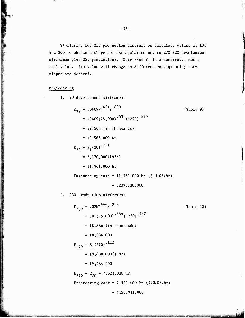
r-

-56-

Similarly, for 250 production aircraft we calculate values at 100

and 200 to obtain a slope for extrapolation out to 270 (20 development

airframes plus 250 production). Note that Y is a construct, not a

real value. Its value will change as different cost-quantity curve

slopes are derived.

Engineering

1. 20 development airframes:

E25 = .0609W631S'82°

= .0609(25,000)•6jl(1250)-820

= 12,566 (in thousands)

= 12,566,000 hr

E20=El(20)-221

= 6,170,000(1938)

= 11,961,000 hr

Engineering cost = 11,961,000 hr ($20.06/hr)

= $239,938,000

2. 250 production airframes:

E = 02W66V987 ^200 °

= .02(25,000)*66A(1250)'987

= 18,886 (in thousands)

= 18,886,000

E270=El(270)-112

= 10,408,000(1.87)

= 19,484,000

E270 " E20 = 7'523»000 hr

Engineering cost = 7,523,000 hr ($20.06/hr)

= $150,911,000

(Table 9)

(Table 12)

"•- -- "■• -: : .- -, V.ttf an ■ • .&,=&*£«*...■,■■:,■■■. ■ ...v..-^^'a. -^ -i.---: ^-- -n| [V -v-ft ,- -fr , ,- ^v,.^^^^. MM^MaAaMMittMMwhMMIü^aHJMMMMM ■nJi L*

-57-

Tooling

1. 20 development airframes:

T25 = .118W727S-508

= 6957 (in thousands)

= 6,957,000 hr

T = T (20)'216

20 V ;

= 3,471,000(1.91)

= 6,629,000 hr

Tooling cost = 6,629,000 hr ($18.63/hr)

= $123,498,000

2. 250 production airframes:

T200 = .522W62V532

= 12,483 (in thousands)

= 12,483,000

T = T (270)'236 270 xiv ;

= 3,575,000(3.748)

= 13,399,000

T270 " T20 = 6.770,000

Tooling cost = 6,770,000 hr ($18.63/hr)

= $126,125,000

(Table 13)

(Table 16)

Nonrecurring Manufacturing Labor

Development Airframes

HMD = .000626W688S1>211

NR

= .000626(25,000)'688(1250)1-211

= 3739 (in thousands)

- 3,739,000 hr

(Table 17)

-58-

Nonrecurring manufacturing labor cost = 3,739,000 hr ($15.77/hr)

= $58,964,000

Recurring Manufacturing Labor

1. 20 development airframes:

H25 = .796W73V258 (Table 22)

= .796(25,000)-735(1250)-258

= 8559 (in thousands)

= 8,559,000 hr

H20 = '^(20),675

= 975,000(7.554)

= 7,365,000 hr

Recurring manufacturing labor cost

2. 250 production airframes:

200 ,582W78Y430

7,365,000 hr ($15.77/hr)

$116,146,000

(Table 25)

78^ 430 = .582(25,000) (1250)

= 34,688 (in thousands)

= 34,688,000 hr

647 H270 = H1(270)

= 1,126,000(37.419)

= 42,134,000

H270 " H20 = 34.769.°00 !ir

Recurring manufacturing labor cost = 34,769,000 hr ($15.77/hr)

- $548,307,000

—~ ; *-~ .-.. ..„ . „ , , - '- -T ■■- rtl •■-"—— M

-59-

Nonrecurring Materials Cost

20 development airframes:

"NR .724 1 924

000024W S

724 1 9?4 = .000024(25,000) (1250) 4

= 33,325 (in thousands)

= $33,325,000

(Table 26)

Recurring Materials

20 development airframes:

M25 - .00478W918S1-004

= .00478(25,000)•918(1250)1-004

= 66,994 (in thousands)

= $66,994,000

699 M20 = M1(20)'

byy

= 7,061,000(8.117)

Cost = $57,317,000

250 production airframes;

M„ 200 - .151W86V813

= .151(25,000)•860(1250)'813

= 301,296 (in thousands)

= $301,296,000

?:>i M270 = Ml(270)

= 5,635,000(66.981)

= 377,440,000

M270 " M20 = $320>123>oco

(Table 27)

(Table 30)

-"■"■*■"■—J-^^**^** —«»A—— - _ - ...-. — i -■—- -MI. ,. ,_ . jUH^gym—- -^ti.-n.H.n, '■■lii i ■

-60-

Flight Test

20 development airirames:

FT - .ISOW-^S^V^DV-1-557 (Table 35)

= . 13(25,000)-71(1250)-586(20r716(l^ 1,55?

= 96,119 (in thousands)

= $96,119,000

Quality Control

20 development airframes:

QC hours = .12 (nonrecurring + recurring labor hours)

= .12(3,739,000 + 7,365,000)

= 1,332,000 hr

QC cost = ($16.33/hr)(1,332,000)

= $22,418,000

250 production airframes:

QC hours .= (.131) (34,769,000)

= 4,172,000

QC cost = ($16.83/hr)(4,207,000)

= $70,215,000

»U - -— - -■ ~-■—--—maüM- m—■ .—. ~—-.~ .,.„,,J_ , , _ _..

-61-

Development Cost (in millions of 1973 $)

Cost Element

Cose Alternative Estimates from

Example Full Sample With Time

Engineering 239 938 Tooling 123 498 Nonrecurring manufac-

turing labor 58 964 Recurring manufac ur-

ing labor 116 146 Nonrecurring manufac-

turing materials 33 325 Recurring manufactur-

ing materials 57 317 Flight test 96 119 Quality control 22 418

Total 744 875

204.31L 346.236

709.443

84.874

77.419

17.^0

837.695

Production Cost

Cost Element

Engineering Tooling Recurring manufactur-

ing labor Recurring manufactur-

ing materials Quality control

Total

Total program

Estimate using total-cost equation

Estimate using Group 2 equation

Cost Alternative Estimates from

Example Full Sample With Time

150.911 126.125

543.307

320.123 70.215

1215.681

1960.555

1947.278

1994.539

126.719

1192.079

1901.522

138.153

406.397

440.571 52.110

1163.856

2001.551

Mt immmmm —

-63-

% % ty *Ö

"Jte :4- '% <^

%, ^ ^>

Appendix B

REGRESSION EQUATIONS AND STATISTICS

■-■— - -———■—- -• -"———-—-■ ■ lull Ml— MMMMMMI MillMM««lll«^—ll. t iMmi iMIlllll—l il in«l«ia»iMnil«lM»

WECEüm PXiS

-65-

Table B-l

BUW-*T n^

ENGINEERING HOURS FOR 25 AIRFRAMES VS WEIGHT, SPEED, TIME

LOG-LINEAR REGRESSION — LN Y * LN A ♦ B * LN XI ♦ C * LN X2 ♦ 0 * LN X3

SUMMARY TABLE

NOTE — STATISTICS ARE BASEO ON LOGARITHMS

LN A •7.40975

A B C D

COEFFICIENT OF COEFFICIENT OF STANOARD ERROR COEFFICIENT OF SUM OF SQUARES

CORRELATION (UNADJUSTED» DETERMINATION (UNADJUSTED) OF THE ESTIMATE OF Y (ADJUSTED» VARIATION (PFRCFNTJ OF Y RESIDUALS

MEAN OF ABSOLUTE ACTUAL PERCENT Y DEVIATIONS DURBIN-WATSON STATISTIC F VALUE DEGREES OF FREEDOM ABOUT REGRESSION CURVE DEGREES OF FREEDOM DUE TO REGRESSION TOTAL OEGREES OF FREFDOM NUMBER OF DATA POINTS

0.60532D-03 0.66231 0.93231 0.77145

0.92012 0.84662 0.36220 4.22815 2.62376

28.90798 2.08770

36.79863 20. 3.

23. 24.

VARIABLES

Y XI X2 X3

CORRELATION

v XI X2 X?

MEANS

MATRIX Y

1.00000 0.70971 0.28478 0.63293

8 .56636 10 .07749 6 .55430 4 .13651

XI 0 .70971 1 ,00000

-0 .33046 0 ,31452

X2 0.28478

-0.33046 l.OOPOO 0.30926

STD DEV

0.86241 1.03004 0.43717 P.26604

X3 0.63293 0.31452 P.30926 1.00000

PARAMETERS STD ERROR T-RATIO LEVEL SIGNIF BETA COEFF

LN B C D

1.67576 0.08771 0.20629 0.33705

•4.42174 7.55089 4.51942 2.28884

-0.99974 1.00000 0.99979 P.96690

0.79104 0.47260 0.23798

- - - _,—

-66-

Table B-2

ENGINEERING HOURS FOR 50 AIRFRAMES VS WEIGHT, SPEED, TIME

LOG-LINEAR REGRESSION — LN V = LN A ♦ 8 * LN XI ♦ C * LN X2 + D ♦ LN X3

SUMMARY TABLE

NOTE — STATISTICS ARE BASEO ON LOGARITHMS

LN A -7.18766

\ 0.755860-03 R 0.67313 r 0.94997 D 0.69765

COEFFICIENT OF CORRELATION (UNADJUSTED) 0.92268 COEFFICIENT OF DETERMINATION (UNADJUSTED) 0.85135 STANDARD ERROR OF THE ESTIMATE OF Y (ADJUSTED) 0.35453 COEFFICIENT OF VARIATION (PERCENT) 4.07137 SUM OF SQUARES OF Y RESIDUALS 2.51389 MEAN OF ABSOLUTF ACTUAL 1 »ERCENT Y DEVIATIONS 27.87806 DURBIN-HATSON STATISTIC 2.23254 F VALUE 38.18009 DEGREES OF FREEDOM ABOUT REGRESSION CURVF 20. DEGREES OF FREEDOM DUE TO REGRESSION 3. TOTAL DEGREES OF FREEDOM 23. NUMBER OF DATA POINTS 24.

VAPIABI ES MEANS STD DEV

Y 8.70800 0.85747 XI 10.07749 1.03004 X2 6.55430 Ü.43717 X3 4.13651 0.26604

CORRELATION MATRIX r XI X2 X3

Y 1.00000 0.71662 0.28405 0.62055 XI 0.71662 1.00000 -0.33046 0.31452 X2 0.28405 -0.33046 1.00000 0.30926 X3 0.62055 0.31452 0.30926 1.00000

PARAMETERS STD ERROR T-RATIÜ LEVEL SIGNIF BETA COEFF

LN A 1.64030 -4.38193 -0.99971 B 0.08586 7.84014 l.OOOOC 0.80859 C 0.20192 4.7C460 0.99986 0.48433 D 0.32992 2.11463 0.95279 0.21645

■ "■■——- - ■-- *_ miiin m —>. ^MMHBaMMMMHMMMHMI^aHaiaaBM^MUEMMaMMd

-67-

Table B-3

ENGINEERING HOURS FOR 100 AIRFRAMES VS WEIGHT, SPEED, TIME

LOG-LINEAR REGRESSION -- LN Y = LN A + B * LN XI ♦ C * LN X2 + D * LN X3

SUMMARY TABLE

NOTE — STATISTICS ARE BASED ON LOGARITHMS

LN A

A B C D

-7.11782

0.81053D-03 0.67225 0.99154 0.64821

COEFFICIENT OF COEFFICIENT OF STANOARO ERROR COEFFICIENT OF SUM OF SyUARES

CORRELATION (UNAOJUSTEC) DETERMINATION I UN ADJUSTED) OF THE ESTIMATE OF V (ADJUSTED) VARIATION (PERCENT) OF Y RESIDUALS

MEAN OF ABSOLUTE ACTUAL PERCENT Y DEVIATIONS DURBIN-WATSON STATISTIC F VALUE DEGREFS OF FREEOOM ABOUT REGRESSION CURVE DEGREES OF FREEDOM DUE TO REGRESSION TOTAL DEGREES OF FREEDOM NUMBER OF DATA POINTS

0.92751 0.86027 0.34034 3.85129 2.31656

25.78494 2.29745

41.04295 20.

3. 23. 24.

VARIABLES

Y XI X2 X3

CORRELATION MATR IX >

Y 1.00000 XI 0.71076 X2 0.30386 X3 0.61754

MEANS

8 0 6 4

.83692 ,07749 ,55430 ,13651

0 I 0 0

XI .71076 ,00000 ,3304b ,31452

X2 0.30386

•0.33046 1.COOOO 0.30926

STD DEV

0.849 00 1.03004 0.43717 0.266 04

X3 0.61754 0.31452 0.30926 1.00000

PARAMETERS STD ERROR

LN B C D

1.5 7460 0.08242 0.19384 0.31670

T-RATIO

4.52039 8.15658 5.11535 2.04673

LEVEL SIGNIF BETA COEFF

-0.99979 1.00000 0.99995 0.94595

0.81560 0.51057 0.20312

. - - -.-■■■ ^. _

-68-

Table B-4

ENGINEERING HOURS FOR 200 AIRFRAMES VS WEIGHT, SPEED, TIME

LOG-LINEAR REGRESSION — LN Y = LN A ♦ B * LN XI ♦ C * LN X2 ♦ 0 * LN X3

SUMMARY TABLE

NOTE — STATISTICS ARF BASED UN LOGARITHMS

LN A -6.74094

A B C D

COEFFICIENT OF COEFFICIENT OF STANDARD ERROR COEFFICIENT OF SUM OF SQUARES

CORRELATION IUNADJUSTEDJ DETERMINATION (UNADJUSTED) OF THE ESTIMATE OF Y (ADJUSTED) VARIATION (PERCENT) OF Y RESIDUALS

MEAN OF ABSOLUTE ACTUAL PERCENT v DEVIATIONS OURBIN-WATSON STATISTIC F VALUE DEGREFS OF FREEDOM ABOUT REGRESSION CURVE DEGREES OF FREEDOM DUE TO REGRESSION TOTAL DEGREES OF FREEDOM NUMBFR OF DATA POINTS

0.118150-02 0.67858 C.99022 0.57481

0.92713 0.85958 0.33784 3.76825 2.28267

25.17930 2.32394

40.80949 20. 3.

23. 24.

VARIABLES

Y XI

X2 X3

CORRELATION

Y XI

X2

X3

MATRIX Y

1.00000 0.71845 0.296't2 0.60264

PARAMETERS STO ERRO

LN A

P

C r

1 0 0 0

.56304 08181 19241 31438

MEANS

8.96535 10.07749 6.55430 4.13651

XI 0.71845 I.00000

■0.33046 0.31452

T-RATIO

4.31271 8.29430 5.14630 1.82842

X2 0.29642

-0.33046 1.00000 0.30V26

STD DEV

0.84P70 1.03004 0.43717 0.26604

X3 0.602 64 0.31452 0.30926 1.00000

LEVEL SIGNIF BETA COEFF

-0.99966 1.00000 P.99995 0.91756

0.83141 0.51492 0.18190

.,...

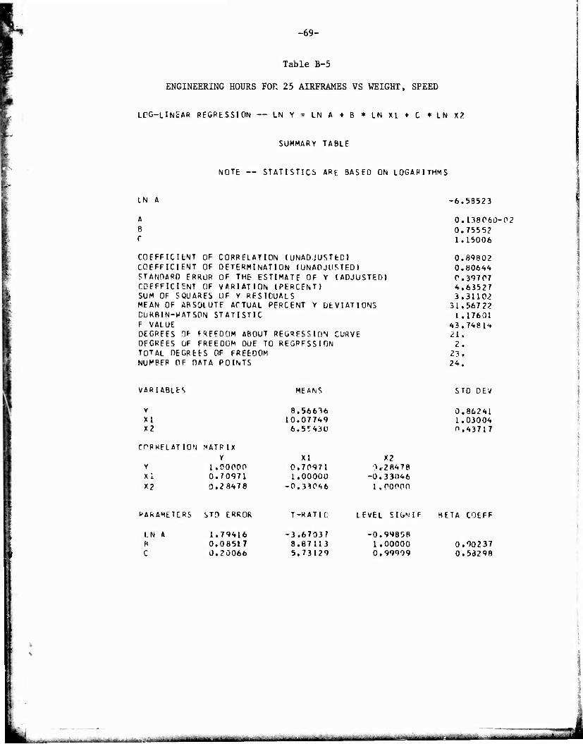
-69-

Table B-5

ENGINEERING HOURS FOR 25 AIRFRAMES VS WEIGHT, SPEED

LCG-LlNcAR REGRESSION — LN Y - LN A ♦ B * LN XI ♦ C * LN X2

SUMMARY TABLE

NOTE — STATISTICS ARE 9ASED ON LOGARITHMS

LN A

A B r

COEFFICIENT OF COEFFICIENT OF STANDARD ERROR COEFFICIENT OF SUM OF SQUARES MEAN OF ABSOLUTE ACTUAL DURBIN-WATSON STATISTIC F VALUE DEGREES OF FREEDOM ABOUT REGRESSION CURVE DFGREES OF FREEDOM DUE TO REGRFSSION TOTAL DEGREES OF FREEDOM NUMBER OF DATA POINTS

CORRELATION (UNADJUSTED) DETERMINATION (UNADJUSTED) OF THE ESTIMATE OF Y (ADJUSTED) VARIATION (PERCENT) UF Y RESIDUALS

PERCENT Y DEVIATIONS

-6.58523

0.13806D-02 0.75552 1.15006

0.89802 0.80644 0.39707 4.63527 3.31102

31.56722 1 .17601

43.7481H

21, 2 •

23. 24.

VARIABLES MEANS STD DEV

Y XI X2

CORRELATION

y Xi X2

MATP IX Y

I.00000 0.70971 0.28478

PARAMETERS STD ERROR

LN A P C

1.79416 0.08517 0.20066

8 10

6

,56636 ,07749 ,5?430

0 1

-0

XI ,70971 .00000 ,33046

T-RATIC;

■3.67037 8.87113 5.73129

0.86241 1.03004 0.43717

X2 3,28478 0.33046 1*00000

EL SICMF BETA COEFF

0.99858 1.00000 0.90237 0.99999 0.53298

if HI ■ in ■■H-"-M rui nn trimft'tfrMt" ■MMja^Mi mmMKM «■■■iniir- - —---*•—--- MMlfe

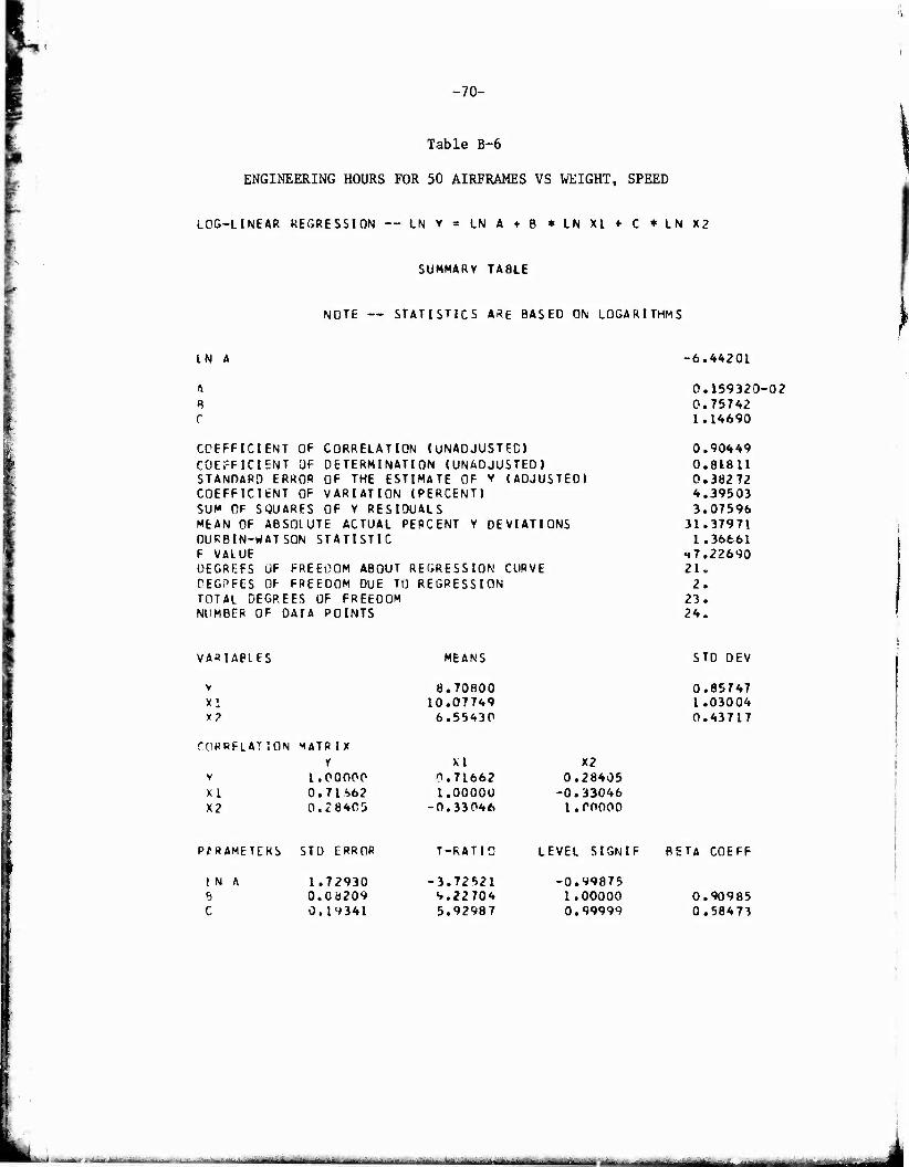
-70-

Table B-6

ENGINEERING HOURS FOR 50 AIRFRAMES VS WEIGHT, SPEED

LOG-LINEAR REGRESSION — LN V = LN A ♦ B * LN XI ♦ C * LN X2

SUMMARY TABLE

NOTE — STATISTICS ARE BASED ON LOGARITHMS

IN A

4

A c

COEFFICIENT OF COEFFICIENT OF STANDARD ERROR COEFFICIENT OF SUM OF SQUARES

CORRELATION (UNAOJUSTEC) DETERMINATION (UNADJUSTED) OF THE ESTIMATE OF V (ADJUSTED) VARIATION (PERCENT) OF Y RESIDUALS

MEAN OF ABSOLUTE ACTUAL PERCENT Y DEVIATIONS DURBIN-WATSON STATISTIC F VALUE DEGREES ÜF FREEDOM ABOUT REGRESSION CURVE DEGREES OF FREEDOM DUE TO REGRESSION TOTAL DEGREES OF FREEDOM NUMBER OF DATA POINTS

-6.44201

0.15932D-02 0.75742 1.14690

0.90449 0.81811 0.38272 4.39503 3.07596

31.37971 1.36661

•♦7.22690 21. 2.

23. 24.

VARIABLES

v XI y?

CriRRELAT ION MATR IX 1

v 1.00000 XI 0.71S62 X2 0.28403

P/.RAMETCKS STD ERROR

MEANS

8.70800 10.07749 6.55430

XI rt.71662 1.00O0Ü

■0.33046

T-RATIO

STD DEV

0.85747 1.03004 0.43717

X2 0.28405 -0.33046 l.POOOO

LEVEL StGNlF BETA COEFF

I N A e c

1.72930 0.08209 0.19341

-3.72521 S.22704 5.92987

-0.99875 I.00000 0.99999

0.90985 0.58473

. in. . HÜ _J

-71-

Table B-7

ENGINEERING HOURS FOR 100 AIRFRAMES VS WEIGHT, SPEED

LOG-LINEAR REGRESSION — IN V = LN A ♦ B * LN XI + C * LN X2

SUMMARY TAELE

NOTE — STATISTICS ARE BASED ON LOGARITHMS

LN A

A B C

COEFFICIENT OF COEFFICIENT OF STANDARD ERROR COEFFICIENT OF SUM OF SQUARES

CORRELATION (UNADJUSTED) DETERMINATION (UNADJUSTED) OF THE ESTIMATE OF Y (ADJUSTED) VARIATION (PERCENT) OF Y RESIDUALS

MEAN OF ABSOLUTE ACTUAL PERCENT Y DEVIATIONS OURBIN-WATSON STATISTIC F VALUE DEGREES OF FREEDOM ABOUT REGRESSION CURVE DEGREES OF FREEDOM DUE TO REGRESSION TOTAL DEGREES OF FREEDOM NUKRER OF DATA POINTS

-6.42502

0.162050-02 0.75057 1.17451

0.91159 0.83100 0.36526 4.13339 2.80178

29.33928 1.44563

51.62931 21, 2.

23. 24.

VARIABLES

Y XI X2

CORRELATION

Y XI X2

MATR IX Y

I.00000 0.71076 0.30386

MEANS

8.83692 10.07749 6.55430

XI 0.71076 1.00000

-0.33046

X2 0.30386

-0.33046 I.COO00

STD DEV

C. 84900 1.03004 0.43717

PARAMETERS STD ERROR

LN B C

1.65043 0.07834 0.18459

T-RATIO

-3.89293 9.58050 6.36285

LEVEL SIGNIF BETA COEFF

-0.99916 1.00000 1.00000

0.91062 0.60478

- —■■ -■ ■ .-i.. ——.. —__«.

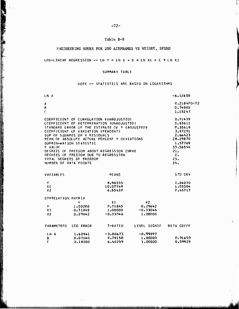
-72-

Table B-8

ENGINEERING HOURS FOR 200 AIRFRAMES VS WEIGHT, SPEED

LOG-LINEAR REGRESSION — IN Y = IN A ♦ B * LN XI ♦ C * LN X2

SUMMARY TABLE

NOTE — STATISTICS ARE BASED ON LOGARITHMS

LN A

A 8 c

COEFFICIENT OF COEFFICIENT OF STANDARD ERROR COEFFICIENT UF SUM OF SQUARES

CORRELATION (UNADJUSTED) DETERMINATION (UNADJUSTED) OF THE ESTIMATE OF v (ADJUSTED) VARIATION (PERCENT) OF Y RESIDUALS

MEAN OF ABSOLUTE ACTUAL PERCENT Y DEVIATIONS DURBIN-WATSON STATISTIC F VALUE DEGREES Of FREEDOM ABOUT REGRESSION CURVE DEGREES OF FREEOOM DUE TO REGRESSION TOTAl OEGREES OF FREEDOM NUMBER OF DATA POINTS

-6.12658

0.21840D-P2 0.74803 1.15247

0.91439 0.83611 C.35619 3.97291 2.66423

28.29870 1.57769

53.56594 21. 2.

23. 24.

VARIABLES

Y XI X2

CORRELATION

Y X! X?

MATRIX Y

1.00000 0.71845 0.29642

MEANS

8.96535 10.07749 6.5543P

XI 0.71845 1.00000

■0.33046

X2 0.29642

-0.33046 1.00000

STD DEV

0.84070 1.03004 0.43717

PARAMETERS STD ERROR T-RAT10 LEVEL SIGNIF BETA COEFF

IN B C

1.60941 0.07640 0.18000

•3.80673 9.79150 6.40259

-0.99897 I.00000 1.00000

0.91650 0.59929

IMmA

-73-

Table B-9

ENGINEERING HOURS FOR 25 AIRFRAMES—SMALL SAMPLE

LOG-LINEAP REGRESSION - IB ! « L8 I ♦ B * IN 11 ♦ C * IB 12

SUMMARY TABLE

NOTE — STATISTICS ARE BASED ON LOGARITHMS

LN ft

A B C

COEFFICIENT OF CORRELATION (UNADJUSTED) COEFFICIENT OF DETERMINATION (UNADJUSTED) STÄNDARD ERROR OF THE ESTIMATE OP I (ADJUSTED) COEFFICIENT OF VARIATION (PERCENT) SUM OF SQUARES OF Y RESIDUALS MEAN OF ABSOLUTE ACTUAL PERCENT Y DEVIATIONS DURBIN-WATSON STATISTIC F VALUE DEGREES OF FREEDOM ABOUT REGRESSION CURVE DEGREES OF FREEDOM DUE TO REGRESSION TOTAL DEGREES OP PREEDOM NUMBER OF DATA PCINTS

MEANS

9.29691 10.36012 6.76955

VARIABLES

Y X1 X2

CORRELATION

Y X1 X2

MATRIX Y

1.00000 C.82995 0.05066

PARAMETERS STD ERROR

LN A B C

2.01170 0.08259 0.21842

X1 0.82995 1.00000

•0.«4U355

T-RATIO

•1.39100 7.64521 3.75601

-2. 79828

0, 60915D-01 0. 631U1 0. 82040

0. 95244 0. 90714 0. 23610 2. 53956 0. 33446

16. 64284 2. 94966

29, 30753 6. 2. 8. 9.

STD DEV

0. 67099 1. 12772 0. 42641

X2 0.05066

-0.44355 1.00000

LEVEL SIGNIF BETA COEFF

-0.78638 0.99974 Ö.99056

1.06119 0.52135

■ ..--..-— LiamM

-74-

Table B-10

ENGINEERING HOURS FOR 50 AIRFRAMES—SMALL SAMPLE

LOG-LINEAR REGRESSION ™ LN Y « LN A ♦ B * LN X1 ♦ C * LN X2

SUMMARY TABLE

NOTE — STATISTICS ARE BASED ON L05ARITHMS

LN A

A B C

COEFFICIENT OF CORRELATION (UNADJUSTED) COEFFICIENT OF DETERMINATION (UNADJUSTED) SfANDARD ERROR OF THE ESTIMATE OF Y (ADJUSTED) COEFFICIENT OF VARIATION (PERCENT) SUM OF SQUARES OF Y RESIDUALS MEAN OF ABSOLUTE ACTUAL PERCENT Y DEVIATIONS D'JRBIN-WATSON STATISTIC P VALUE DEGREES C? FREEDOM ABOUT REGRESSION CURVE DE3REES OF FREEDOM DUE TO REGRESSION TOTAL DEGRESS CF FREEDOM NUMBER OF DATA POINTS

VARIABLES

Y X1 X2

CORRELATION

Y XI X2

MATRIX Y

1.0C000 0.81082 C.08855

MEANS

9.U2365 10.36012 6.76955

X1 0.81082 1.00000

-0.4«355

12 0.08855

•0.44355 1.00000

-3 31413

0. 36366C-01 0. 64335 0. 89705

0. 95263 0. 90751 0. 24074 2. 55465 0. 34774

17. 67481 2. 83757

29. 43605 6. 2. 8. 9.

STD DEV

0. 68554 1. 12772 0. 42641

PARAMETERS STD ERROR

LN B C

2.05124 0.08421 0.22272

T-RATIO

-1.61567 7.63960 4.02777

LEVEL SIGNIF BETA COEFF

-0.84271 0.99974 0.99310

1.05831 0.55797

r ..I... I ■ ■ , - - ^™^

-75-

Table B-ll

ENGINEERING HOURS FOR 100 AIRFRAMES--SMALL SAMPLE

L03-LINEAR REGRESSION — LN Y = LN A ♦ B * LN X1 ♦ C * LN X2

SUMMARY TABLE

NOTE STATISTICS ARE BASED ON LOGARITHMS

LN A

A B C

COEFFICIENT OF CORRELATION (UNADJUSTED) COEFFICIENT OF DETERMINATION (UNADJUSTED) STANDARD EPROR OF THE ESTIMATE OF r (ADJUSTED) COEFFICIENT OF VARIATION (PERCENT) SOI! OF SQUARES OF Y RESIDUALJ MEAN OF ABSOLUTE ACTUAL PERCENT Y DEVIATIONS DURBIN-WATSON STATISTIC F VALUE DEGREES OF FREFDOM ABOUT REGRESSION CURVE DEGREES OF FREEDOM DUE TO REGRESSION TOTAL DEGREES OF PRBEDOH NUMBER OF DATA POINTS

VARIABLES

Y X1 X2

CORRELATION MATRIX Y

Y 1.00000 X1 0.79079 X2 0.11502

MEANS

9.54080 10.36012 6.76955

XI 0.79079 1.00000

-0.41*355

12 0. 11502

-0.44355 1.00000

-3 75348

0. 23436C-01 0. 65598 0, 95992

0. 94627 0. 89543 0. 26357 2. 76259 0. 41682

18. 85491 2. 61251

25. 69028 6. 2. 8. 9.

STD DEV

0. 70589 1. 12772 0. 42641

PARABETKRS STD ERROR

LN B C

2.24578 0.09220 0.24384

T-BATIO

-1.67135 7.11487 3.93670

LEVEL SIGNIF BETA COEPF

•0.85431 0.99961 C.99235

1.04799 0.57986

-■ ...~■...-.... ,,.„,, ,,. MüaaM«« ■l I l «.Uli ».t. , ■in

-76-

Table B-12

ENGINEERING HOURS FOR 200 AIRFRAMES--SMALL SAMPLE

LOG-LINEAR REGRESSION — LN Y = LH A ♦ B * LN 11 ♦ C * LN 12

SUHHARY TABLE

NOTE — STATISTICS ABE BASED ON LOGARITHMS

LN A

A B C

COEFFICIENT OF CORRELATION (UNADJUSTED) COE'FICISST OP DETERMINATION (UNADJUSTED) STANDARD ERROR OF THE ESTIMATE OF Y (ADJUSTED) COEFFICIENT OF VARIATION (PERCENT) SUM OF SQUARES OF Y RESIDUALS MEAN OF ABSOLUTE ACTUAL PERCENT Y DEVIATIONS DURBIN-WATSON STATISTIC F VALUE DEGPEES OF FREEDOM ABOUT REGRESSION CURV5 DE3REES OF FRBEDOH DUE TO REGRESSION TOTAL DEGREES CF FREEDOM MJHBER OF DATA POINTS

-3.91041

0.20032D-01 0.66360 0.98708

0.94161 0.88663 0.27936 2.89596 0.46826 19.37525 2.44382

23.46196 6. 2. 8. 9.

VARIABLES HEANS STD DEV

Y X1 X2

CORRELATION MATRIX Y

Y 1.00000 X1 0.78167 X2 0.12182

PARAMETERS STD ERROR

LN A B C

2.38033 0.C9772 0.25845

9.64666 10.36012 6.76955

C.71854 1.12772 0.42641

X1 0.78167 1.00000

-0.44355

12 0.12382

-0.44355 1.00000

T-RATIO LEVEL SIGNIF BETA C01FF

-1.64280 6.79062 3.8193C

-0.84847 0.99950 0.99123

1.04149 0.58577

^BU^MI ^^tummtmmmmmasaimmtaammtiiemmm tammmmm

-77-

Table B-13

TOOLING HOURS FOR 25 AIRFRAMES

LOG-LINEAR REGRESSION -- IN V = LN A ♦ B * LN XI ♦ C * LN X2

SUMMARY TABLE

NOTE — STATISTICS ARE BASEC ON LOGARITHMS

LN A -2.13739

A 0.11796 R

C 0.72713 0.50821

COEFFICIENT OF CORRELATION 'UNADJUSTED) 0.85777 COEFFICIENT OF DETERMINATION «UNADJUSTED) 0.73577 STANDARD ERROR OF THE ES'' IMATE OF Y lAOjUSTED) P.44000 COEFFICIENT OF VARIATION (PERCENT) 5.17830 SUM OF SQUARES OF Y RESIDUALS 4.25915 riEAN Hc ABSOLUTE ACTUAL °ERCENT Y DEVIATIONS 34.62077 OURRIN-WATSON STATISTIC 2.15045 F VALUE 3P. 62968 DEGREES OF FREEDOM ABOUT REGRESSION CURVE 22. DEGREES OF FREEDOM DUE TC ) REGRESSION c •

TOTAL DEGREES OF FREEDOM 24. NUMBER OF DATA POINTS 25.

VARIABt ES MEANS STD DEV

V 8.49695 0.81952 XI 10.04881 1.01849 X2 6.54767 P.42925

CORRELATION MATR IX Y XI X2

v I.COOOP 0.81973 -0.0187: XI 0.81973 1.00000 -0.31532 ■ > -0.01870 -0.31532 1.COPOP

PARAMETER STO ERROR T-R^TI" LEVEL SIGN IF PETA COEFF

LN A 1.95294 -1.09445 -0.71440 B 0.09292 7.82496 1.00000 P.90366 r 0.220*8 2.30495 0.96902 0.26619

_^_ M

-78-

Table B-14

TOOLING HOURS FOR 50 AIRFRAMES

LOG-LINEAR REGRESSION — LN Y = LN A ♦ B * LN XI ♦ C * LN X2

SUMMARY TABLE

NOTF — STATISTICS ARE BASEO ON LOGARITHMS

LN A

a p c

COEFFICIENT OF CUEFFICIFNT OF STANDARD ERROR COEFFICIENT OF SUM OF SQUARES

CORRELATION (UNADJUSTEDl DETERMINATION (UNADJUSTED» OF THE ESTIMATE OF Y (ADJUSTED» VARIATION (PERCENT) OF Y RESIDUALS

MFAN OF ABSOLUTE ACTUAL PERCENT Y DEVIATIONS DURPIN-WATSON STATISTIC F VALUE DEGREES OF FREEDOM ABOUT REGRESSION CURVE DEGkFES OF FREEDOM DUE TO REGRESSION TOTAL DEGREES OF FREEDOM NUMBER OF DATA POINTS

-l.lMtO

0.30806 0.67377 0.47912

0.8*855 0.72004 0.42418 4.85872 3.95838 33.49742 2.17645

28.29192 22. 2.

24. 25.

VARIABLES

v XI X2

CORRELATION MATft IX

v XI X2

1.00000 0.80956

-0.01397

MEANS

8.73023 10.04881 6.54767

XI 0.80<»56 1.00000

-0.31532

X2 -0.01397 -0.31532

1.00000

STD DEV

0.J6755 1.01849 0.42925

(-'ARAMETERS STD ERROR

I N P f

1.88273 0.08958 0,21256

T-RATIP

-0.62541 7.52120 2.25407

LEVEL SIGNIF BETA COEFF

-0.46186 1.00000 ^96551

Ü; 89405 0.26794

-79-

Table B-15

TOOLING HOURS FOR 100 AIRFRAMES

LCG-LINEAR KFGRESSION -- LN Y = LN A ♦ B * LN XI + C * LN X?.

SUMMARY TABLE

NOTE ~ STATISTICS ARC BASED ON LOGARITHMS

LN A

A P C

COEFFICIENT OF COEFFICIENT OF STANDARO ERROR COEFFICIENT OF SUM OF SQUARES

CORRELATION (UNADJUSTED) DETERMINATION (UNAOJUSTED) OF THE ESTIMATE OF Y (ADJUSTED) VARIATION (PERCFNT) OF Y RESIDUALS

MEAN OF ABSOLUTE ACTUAL PERCENT Y DEVIATIONS DURB1N-WATS0N STATISTIC F VALUE DEGREES OF FREEDOM ABOUT REGRESSION CURVE DFGRFES OF FREEOOM DUE TO REGPESSIUN TOTAL DEGREES OF FREEDOM NUMBER OF DATA POINTS

-0.73015

0.47229 0.63801 0.49908

0.04172 0.70849 0.41319 4.62751 3.75589 32.75785 2.28926

2t>. 73501 22.

•) *-. 24. 25.

VARIABLES MEANS STD DEV

Y XI X2

8.92889 10.04881 6.54 767

0.732 70 1.01849 0.42925

CORRELATION

Y XI X2

MATR IX Y

I.00000 0.79467 0.01273

XI 0.79467 1.00000

-0.31532

X2 0.01273

-0.31532 I.00000

PARAMETERS STD ERROR T-RATIO LEVEL S1GNIF 0ETA COEFF

LN A B r

1.83394 0.08726 0.20705

-P.40904 7.31148 2.41043

-0.31354 1.00000 0.97527

0.886e> 0.29238

-80-

Table B-16

TOOLING HOURS FOR 200 AIRFRAMES

LOG-IINEAR REGRESSION — LN Y = IN A ♦ B * LN XI + C * LN X2

SUMMARY TABLE

NOTE — STATISTICS APE BASED ON LOGARITHMS

LN A

A P C

COEFFICIENT OF COEFFICIENT OF STANOAPD ERROR COEFFICIENT UF SUM OF SQUARES

CORRELATION (UNADJUSTED) DETERMINATION (UNADJUSTED! ÜF THE ESTIMATE OF Y (ADJUSTED) VARIATION (PERCENT) OF Y RESIDUALS

MEAN OF ABSOLUTE ACTUAL PERCENT Y DEVIATIONS DURBIN-WATSON STATISTIC f VALUE DEGREES OF FREEDOM ABOUT REGRESSION CURVE DEGREES Or FREEDOM DUE TO REGRESSION TOTAL DEGREES OF FREEDOM KUMBFP OF DATA POINTS

-0.64933

0.522 39 0.62136 0.53225

0.83620 0.69924 0.41187 4.53619 3.73199

33.20448 2.16504

25.57366 22. 2.

24. 25.

VARIABLES

Y XI X2

CORRELATION MftTR IX V

Y 1.00000 XI 0.77995 X? 0.04021

MEANS

9.07961 10.04881 6.54767

XI 0.77995 l.OOPOO •0.31532

X2 0.04021 -0.31532 1.00000

STD DEV

0.71904 1.01849 0.42925

PARAMETERS STD LRRÜR

IN A

I

1.82809 0.08698 0.20639

T-RAriC)

•0.35520 7.14346 2.57885

LEVEL SIGNIF BETA COEFF

-0.2 7417 1.00030 U.9i287

0.88014 0.31774

-81-

Table B-17

NONRECURRING MANUFACTURING LABOR HOURS

LOG-LINEAR REGRESSION « LN Y = LN A ♦ B * LN XI ♦ C * LN X2

SUMMARY TABLE

NOTE -- STATISTICS ARE BASED ON LOGARITHMS

LN A

A R r

COEFFICIENT OF COEFFICIENT OF STANDARD ERROR COEFFICIENT OF SUM OF SQUARES

CORRELATION (UNADJUSTED) DETERMINATION (UNADJUSTED» OF THE ESTIMATE OF Y (AOJUSTEÜ) VARIATION (PERCENT) OF Y RESIDUALS

MEAN OF ABSOLUTE ACTUAL PERCENT Y DEVIATIONS DUPBIN-WATSON STATISTIC F VALUE DEGREES OF FREEDOM ABOUT REGRESSION C'.'RVE DEGREES OF FREEDOM OUE TO REGRESSION TOTAL DEGREES OF FREEDOM NUMBER CF DATA POINTS

-7.37620

0.62597D- C.68833 1.21089

0.72627 P. 52747 0.72442 9.66285

11.02044 60.30124

2.62561 11.72065 21. 2.

23. 24.

03

VARIABLES

Y XI X2

CORRELATION

XI X?

MATRIX v

I.00000 0.53037 0.29302

MEANS

7.49695 10.07749 6.55430

XI 0.5303? 1.00000

-0.33046

X2 0.293 32

■0.33046 1.OOOJO

STD OEV

1.00698 ].03004 0.^3717

PARAMETERS STD ERROR

LN R

C

3.27325 0.15538 0.36609

T-RATIO

•2.25348 4.43007 3.30763

LEVEL SIGN IF ft ETA COEFF

-0.96496 0.99977 0.99665

0.70409 0.52 5 70

_

-82-

Table B-18

RECURRING MANUFACTURING LABOR HOURS FOR 25 AIRFRAMES VS WEIGHT, SPEED, TIME

LOG-LINEAR REGRESSION — LN V = LN ft ♦ B * LN X1 ♦ C * LN X2 ♦ 0 * LN X3

SUMMARY TABLE

NOTE — STATISTICS ARE BASED ON LOGARITHMS

LN A 0.73180

A B C ,')

COEFFICIENT OF CORRELATION (UNADJUSTED) COEFFICIENT OF DETERMINATION (UNADJUSTED) STANDftPO FRRGR OF THF ESTIMATE OF Y (ADJUSTED) COEFFICIENT OF VARIATION (PERCENT) SUM OF SQUARES OF V RESIDUALS MEAN OF ABSOLUTE ACTUAL PERCENT Y DEVIATIONS nURHlN-WATSON STATISTIC r VALUE DECREES <)F FREEDOM ABOUT REGRESSION CURVE DEGREES OF rREfcÜOM DUE TO REGRESSION TDTAl DEGREES OF FREEDOM NUMBER OF DATA POINTS

2.07882 0.798 74 0.41443

-0.63285

0.91459 0.83647 0.34866 3.942 66 2.55288

28.27553 2.67711

35.80594 21. 3.

24. 25.

VARIABLES MEANS SID DEV

Y XI X? X3

CORRELATION

Y X 1 X2 > 3

MATR I X Y

I.00000 0.d8470

-0.I 5544 0.10073

8.84334 10.04381 6.54767 4.15321

XI 0.88470 1.00000

•0.31532 0.25356

X2 -0. 15544 -J.3153? l.COOOO 0.270J5

0.80652 1.01849 0.42925 0.27349

X3 0.10073 0.25356 0.27005 1.00000

PARAMETERS STD FRRÜR

I N A c

c D

1.60929 0.0792P 0.18899 0.29101

T-RATIC

0.^474 10.07444 2.19234

-2.17468

LEVEL SIGNIF BETA COEFF

0.34604 1.00000 0.96028

-0.95877

1 .00867 0.22057

-0.21460

-83-

Table B-19

RECURRING MANUFACTURING LABOR HOURS FOR 50 AIRFRAMES VS WEIGHT, SPEED, TIME

LOG-LINEAR REGRCSSICN — LN Y = IN A + B * LN X1 + C * LN X2 + D * LN X3

SUMMARY TABLE

NOTE — STATISTICS AkE BASED ON LOGARITHMS

LN A 0.36577

A 1.44163 B 0.81655 c 0.48453 D -0.59477

COEFFICIENT OF CORRELATION (UNADJUSTED) 0.92877 COEFFICIENT OF DETERMINATION (UNADJUSTED) 0.86261 STANDARD ERROR OF THE ESTIMATE Oh Y (ADJUSTED) 0.32080 COEFFICIENT OF VARIATION (PERCENT) 3.45936 SUM OF SQUARES OF Y RESIDUALS 2.16117 MEAN OF ABSOLUTE ACTUAL PERCENT Y DEVIATIONS 26.11730 DURBIN-WATSÜN STATISTIC 2.59723 F VALUE 43.95139 DEGREES OF FREEDOM ABOUT REGRESSION CURVE 21. DEGREES OF FREEDOM DUE TU REGRESSION 3. TOTAL DEGREES OF FREEDOM 24. NUMBER OF DATA POINTS 25.

VARIABLES MEANS STO DEV

Y 9.27340 0.80960 XI 10.04881 1.01849 X2 6.54 767 0.42925 X3 4.15321 0.27349

CORRELATION MATRIX Y XI X2 X3

Y 1.00000 0.89529 -0. 12127 0.12893 XI 0.Ö9529 I.00000 -0. 31532 0.25356 X2 -0.1 127 -0.31532 1, 00000 0.27005 X3 0.12893 0.25356 0. 27005 1.00000

PARAMETERS STD ERROR T-RAT10 LEVEl SIGNIF BETA COEFF

LN A 1.48069 0.24703 0. 19271 R 0.07295 11.19358 1. 00000 1.02724 C 0.17389 2.78639 0. 98894 0.25690 0 0.26776 -2.22133 -0. 96254 -0.20092

-84-

Table B-20

RECURRING MANUFACTURING LABOR HOURS FOR 100 AIRFRAMES VS WEIGHT, SPEED, TIME

LOG-LINEAR «EGRESSION -- LN Y = LN A ♦ B * LN XI ♦ C * LN X2 ♦ D * LN X3

SUMMARY TABLE

NOTE ~ STATISTICS ARE BASED ON LOGARITHMS

LN A -0.22987

COEFFICIENT OF COEFFICIENT OF STANDARD ERKUR COEFFICIENT OF SUM OF SQUARES

CORRELATION (UNADJUSTED) DETERMINATION (UNADJUSTED! OF THE ESTIMATE OF Y (ADJUSTED) VARIATION (PERCENT) OF Y RESIDUALS

MEAN OF ABSOLUTE ACTUAL PERCENT Y DEVIATIONS DURBIN-WATSON STATISTIC F VALUE DEGREES OF FREEDOM ABOUT REGRESSION CURVE DEGREES OF FREEDOM DUE TO REGRESSION TOTAL DEGREES OF FREEDOM NUMBER OF DATA POINTS

0.79464 0.846 88 0.55507

-0.53478

0.93452 0.87332 0.31793 3.27976 2.1226t

25.53876 2.60290

48.25851 21. 3.

24. 25.

VARIABLES MEANS STD DEV

Y XI X2 X3

CORRELATION

Y XI X2 X3

MATRIX Y

I.00000 0.89798

-0.08762 0.16372

9.69367 10.04881 6.54767 4.15321

XI 0.89798 1.00000

-0.31532 0.25356

X2 -0.08762 -0.31532

1.00000 0.27005

0.83557 1.01849 0.42925 0.27349

X3 0.16372 0.2?356 0.27005 1.00000

PARAMETERS STD ERROR

IN B C D

1.46743 0.07229 0.17233 0.26536

T-RATIO

-0.15664 11.71428 3.22090

-2.01530

LEVEL SIGN1F BETA COEFF

-0.12298 1.00000 0.99590

-0.94315

1.03228 0.28515

-0.17503

_ .. ... . ........

-85-

Table B-21

RECURRING MANUFACTURING LABOR HOURS FOR 200 AIRFRAMES VS WEIGHT, SPEED, TIME

LOG-LINEAR REGRESSION -- LN Y = LN A ♦ B * LN XI ♦ C * IN X2 ♦ D * LN X3

SUMMARY TABLE

NUTF — STATISTICS APE BASED ON LOGARITHMS

LN A 0.17265

A 1.18845 H 0.83062 C 0.54636 0 -0.47113

COEFFICIENT OF CORRELATION (UNADJUSTED) 0.93786 COEFFICIENT OF DETERMINATION (UNADJUSTED) 0.87959 STANDARD ERROR OF THE ESTIMATE OF Y (ADJUSTED) 0.30397 COEFFICIENT OF VARIATION (PERCENT) 2.99770 SUM OF SQUARES OF Y RESIDUALS 1.94031 MEAN OF ABSOLUTE ACTUAL PERCENT Y DEVIATIONS 24.29084 DUPBIN-WAT SON STATISTIC 2.43985 F VALUE 51.13307 DEGREES OF FREEDOM ABOUT REGRESSION CURVE 21 . DEGREES OF FREEDOM DUE TO REGRESSION 3. TTTAL DEGREES OF FREEDOM 24. NUMBER OF DATA POINTS 25.

VARIABLES MEANS STO l)EV

Y 10.14000 0.81939 XI 10.04881 1.01849 X2 6.54767 0.42925 X3 4.15321 0.27349

CORRELATION MATRIX Y XI X2 X}

Y I.00000 0.90232 -0. C61B0 0.18183 XI 0.90232 1.00000 -P. 31532 0.25356 *2 -o.Oöieo -0.31532 1. cocoo 0,27005 X3 0.16183 0.25356 0 27005 1.00000

PARAMETERS STD ERROR T-RATIO LEVEL SIGN IF BETA COEFF

L N A 1.40299 0.12306 0, 09677 R 0.06912 12.01704 1. 00000 1.03244 C P.16477 3.31596 0 99672 0.28621 D 0.25370 -1.85701 -0. 92261 -0.15725

.... ...... ...-. ,........ . .. ._ - -.^1... :■, „ ^.c.^^i. . i. ... -._-.. ."7-..

-86-

Table B-22

RECURRING MANUFACTURING LABOR HOURS FOR 25 AIRFRAMES VS WEIGHT, SPEED

LOG-LINEAR REGRESSION -- LN Y = LN A + B * LN XI + C * LN X2 .

SUMMARY TABLE

NOTE — STATISTICS APE BASED ON LOGARITHMS

LN A

A R C

COEFFICIENT ÜF COEFFICIENT OF STANDARD ERROR COEFFICIENT OF SUM PF SQUARES

CORRELATION (UNADJUSTED) DETERMINATION (UNADJUSTED» OF THE ESTIMATE OF Y (ADJUSTED) VARIATION (PERCENT) OF Y RESIDUALS

MEAN OP ABSOLUTE ACTUAL PERCENT Y DEVIATIONS DURBIN-HATSON STATISTIC F VALUE DEGREES OF FREEDOM ABOUT REGRESSION CURVE DEGREES OF FREEDJn 1UE TO REGRESSION TOTAt DEGREES OF FREEDOM NUMBER OF DATA POINTS

VAPIABLFS

Y XL X2

COPRFLATION

Y

X2

MATR IX Y

I.OOOOO 0.88*70

-0.15544

PABA",FTFRS STD FRROR

I N A R

r

1.67358 0.07963 0.18895

MEANS

8.84334 10.04881 6.54767

XI 0.88470 1.00000

-0.31532

T-RATIO

■0.13639 9.22777 L.36402

-0 ,22825

0 .79592 0 .73482 0 .25773

0 .89423 0 .79964 0 .37706 4 .26375 3 .12779

31 .74411 2 ,55514

43 •902J6 22 2 >

24 » 25 1

STD DEV

0 80652 1 ,01849 0 ,42925

X2 -0.15544 -0.31532 1.00000

VEL SIGNIF BETA CÜEFF

-0.10724 1.00000 0.92796 0.81365 0.13717

-87-

Table B-23

RECURRING MANUFACTURING LABOR HOURS FOR 50 AIRFRAMES VS WEIGHT, SPEED

LOG-LINEAR REGRESSION — LN Y = I N A ♦ 8 * LN XI ♦ C * LN X2

SUMMARY TABLE

NOTE ~ STATISTICS ARE BASED ON LOGARITHMS

LN A -0.53651

A 0.584 78 P 0.75648 C 0.33725

COEFFICIENT OF CORRELATION «UNADJUSTED! 0.91123 COEFFICIENT OF DETERMINATION (UNADJUSTED» 0.83033 STANOARO ERROR OF THE ESTIM4TE OF Y (ADJUSTED) 0.34831 COEFFICIENT OF VARIATION (PERCENT) 3.75597 SUM OF SQUARES OF Y RESIDUALS 2.66897 MEAN OF ABSOLUTE ACTUAL PERCENT Y DEVIATIONS 29.41340 OURBIN-WATSON STATISTIC 2.53640 F VALUE 53.83289 DEGREES OF FREEDOM ABOUT REGRESSION CURVE 22. DEGREES OF FREEDOM DUE TC ) REGRESSION ?.. TOTAL DEGREES OF FREEDOM 24. NUMBER OF DATA POINTS 25.

VARIABLES MEANS STD DEV

Y 9. 273*0 0.80960 XI 10.04881 1.01849 X2 6.54767 0.42925

CORRELATION MATRIX Y XI X2

Y 1.00000 0.89529 -0. 12127 XI 0.89529 1.00000 -0. 31532 X2 -0.12127 -0.31532 1. 00000

PARAMETERS STD ERROR T-RATIO LEVEL SIGNIF BETA COEFF

LN A 1.54597 -0.3470* -0. 26814 B 0.07356 10.28391 1. 00000 0.95167 C 0.17454 1.93225 0. 93369 0.17881

-88-

Table B-24

RECURRING MANUFACTURING LABOR HOURS FOR 100 AIRFRAMES VS WEIGHT, SPEED

LOG-LlNEAR REGRESSION — LN V = IN A + B * LN XI ♦ C * LN Xi

SUMMARY TABLE

NOTE — STATISTICS ARE BASED ON LOGARITHMS

LN A -1.04113

A 0.35305 P C

0.792 87 0.42265

COEFFICIENT OF CORRELATION (UNADJUSTED) 0.92132 COEFFICIENT OF DETERMINATION (UNAOJUSTED) 0.848 82 STANDARD ERROR OF THE ESTIMATE OF Y (AOJUSTED) 0.33933 fOEFFICIENT OF VARIATION (PERCENT) 3.50053 SUM OF SQUARES OF Y RESIDUALS 2.53318 MEAN OF ABS OLUTE ACTUAL PERCENT Y DE VIATIONS 27.65469 DURBIN-WATSON STATISTIC 2.56989 F VALUE 61.76243 DEGREES OF FREEDOM ABOUT REGRESSION CURVE 22. DFGREES OF FREEDOM DUE TO REGRESSION 2. TOTAL DEGREES OF FREEDOM 24. NUMBER OF DATA POINTS 25.

VARIABLES MEANS STD DEV

Y 9.69367 0.83557 XI 10.04881 1.01849 X2 6.54767 0.42925

CORRELATION MATRIX Y XI X2

Y 1.00000 0.89798 -0.08762 XI 0.89798 I.00000 -0.31532 X2 -0.08762 -0.31532 1.00000

PARAMETERS STD ERROR T-RATIO LEVEL SIGNIF BETA COEFF

LN A 1.50613 0.69127 -0.50337 B 0.07166 11.06380 1.00000 0.966 - r. 0.170C4 2.48559 0.97898 0.2171 .

-89-

Table B-25

RECURRING MANUFACTURING LABOR HOURS I OR 200 AIRFRAMES VS WEIGHT, SPEED

LOG-LINeAR REGRESSION -- LN Y = LN A ♦ B * LN XI ♦ C * LN X2

SUMMARY TABLE

NOTE -- STATISTICS ARE BASED ON LOGARITHMS

LN A

A P C

COEFFICIENT OF

COEFFICIENT OF STANDARD ERROR COEFFICIENT OF SUM OF SQUARES

CORRELATION (UNADJUSTED)

DETERMINATION (UNADJUSTED) OF THE ESTIMATE OF Y (ADJUSTED) VARIATION (PERCENT) OF Y RESIDUALS

MEAN OF ABSOLUTE ACTUAL PERCENT Y DEVIATIONS DUPBIN-HATSON STATISTIC

F VALUE DEGREES OF FREEDOM ABOUT REGRESSION CURVE DEGREES OF FREEDOM DUE TO REGRESSION TOTAL DEGREES OF FREEDOM NUMBER OF DATA POINTS

-0.54207

0.58155 Ü. 78303 0.42970

0.92726 Ö.85981 0.32044 3.16011 2.25893

25.88412 2.44790

67.46665 22. 2.

24. 25.

VARIABLES MEANS STD DEV

Y XI X2

CHRRtLATION

Y XI X?

MATR IX V

I.00000 0.90232

-0.08180

10.14000 10.04881 6.54767

xi 0.90232 1.00000

-0.31532

X2 -0.C8180 -0.31532 1.00000

0.81939 1.01849 0.42925

PARAMETERS STD ERROR

LN R r

1.42226 0.06767 0.16057

r-RATIO

-0.38113 11.57079 2.67603

LEVEL SIGNIF BETA COfcFF

-0.29324 1.00000 0.98620

0.97330 0.22510

■

-90-

Table B-26

NONRECURRING MATERIALS COST VS WEIGHT AND SPEED

LOG-LINEAR DEGRESSION -- LN Y « IN A t B * LN XI ♦ C * LN X?

SUMMARY TABLE

NOTE — STATISTICS ARF BASED ON LOGARITHMS

LN A 10.63540

COEFFICIENT OF COEFFICIENT OF STANDARD ERROR COEFFICIENT UF SUM OF SQUARES

CORRELATION (UNADJUSTED) DETERMINATION (UNADJUSTED) OF THE ESTIMATE OF Y (ADJUSTED) VARIATION (PERCENT) OF Y RESIDUALS

MEAN OF ABSOLUTE ACTUAL PERCENT Y DEVIATIONS nURRlN-WATSUN STATISTIC F VALUE DEGREES OF FREE.' 80UT REGRESSION CURVE DEGREES OF f-REEi > 'JE TO REGRESSION TOTAL DEGREES V JDOM NUMBER OF DATA PüiiMfS

0.240*90-04 0.72404 1.92395

0.82660 0.68326 0.66487 7.18399 9.28313 51.42606 2.17561

22.65064 21.

2. 23. 24.

VARIABLES MEANS STO DEV

Y XI v?

9.25491 10.04739 6.55712

1.12885 1.04037 0.43581

CORRELATION MATR IX y

Y 1.00000 XI 0.43222 X2 0.53158

XI 0.43222 I.00000 0.31649

X? 0.53158 -0.31649 1.00000

PAPAMFTERS STD ERROR T-RATIO LEVEL SIGNIF BETA COEFF

LN A B r

2.96820 0.14048 0.33535

■3.58311 5.15420 5.73720

-0.99825 0.99996 0.99999

0.66730 0.74273

-91-

Table B-27

RECURRING MATERIALS COST FOR 25 AIRFRAMES VS WEIGHT, SPEED

LOG-LINEAR REGRESSION — LN v = LN A ♦ 9 * LM! » C * LN X2

SUMMARY TABLE

NUTE — STATISTICS A«E BASED ON LOGARITHMS

LN A

A R C

CORRELATION (UNADJUSTED» DETERMINATION (UNADJUSTED) OF THE ESTIMATE OF Y (AOJUSTEO) VARIATION (PERCENT) OF Y RESIDUALS

PERCENT Y DFVIATIONS

COEFFICIENT OF COEFFICIENT OF STANDARD ERROR COEFFICIENT OF SUM OF SQUARES MEAN OF ABSOLUTE ACTUAL DURBIN-WATSON STATISTIC F VALUE DEGREES OF FREEDOM ABOUT REGRESSION CURVE DEGREES OF FREEDOM DUE TO REGRESSION TOTAL DEGREES OF FREEDOM NUMBER OF DATA POINTS

VARIABLES

v XI X?

CORRELATION

v

Xf X2

MATH IX Y

I.00000 0.81820 0.13981

MEAK'S

10.45757 10.0*881 6.5*767

XI 0.8182P I.00000 •0.31532

X2 0.13981 -0.31532 1.00000

-5 ,342 36

0 .478460-02 0 .91774 1 .00459

0 .91933 0 .84517 0 .40120 3 .83647 3 ,54118

33 ,02686 I .45026

60 .046 56 22 1

2 1

24 25

STD DEV

0 97621 I 01849 0 42925

PARAMETERS STD ERRGR

LN A B r.

1.78075 0.08473 0.20104

T-RATIO

-3.00006 10o83124 4.99688

LEVEL SfGNIF BETA COEFF

-0.99341 I.00000 0.99995

0.95749 0.44173

-92-

Table B-28

RECURRING MATERIALS COST FOR 50 AIRFRAMES VS WEIGHT, SPEED

LOG-LINEAR REGRESSION -- LN Y = LN A ♦ B * LN XI ♦ C * LN X2

SUMMARY TABLE

NOTE — STATISTICS ARE BASED ON LOGARITHMS

LN A

A P

C

COEFFICIENT OF COEFFICIENT OF STANDARD ERROR COEFFICIENT OF SUM Of SQUARES

CORRELATION (UNADJUSTFO) DETERMINATION (UNADJUSTED) OF THE ESTIMATE OF Y «ADJUSTED) VARIATION (PERCENT) OF Y RESIDUALS

MEAN OF ABSOLUTE ACTUAL PERCENT Y DEVIATIONS

PUR6IN-WATS0N STATISTIC F VALUE DEGREES OF FREEDOM ABOUT REGRESSION CURVE DEGREES OF FREEDOM DUE TO REGRESSION TOTAL OEGFEES OF FREEDOM MUMBcR OF DATA POINTS

-4.1*315

0.158730-01 P.90023 0.92882

0.92567 0.85686 0.3T437 3.40810 3.08336

30.69236 1.44044

65.84939 22. 2.

24. 25.

VARIABLES

Y XI X2

CORRELATION

Y XI X2

MATRIX Y

1.00000 0.83509 0.11567

MEANS

10.98469 10.04881 6.54767

XI 0.83509 I.00000

-0.31532

X2 0.11567

-0.31532 l.COOOO

STD DEV

0.94739 1.01849 0.42925

PARAMETERS STD ERROR

IN A B r

1.66165 0.07906 0.18760

T-RATIO

-2.49339 11.38606 4.951'3

LEVEL SIGNIF BETA CUEFF

-0.97934 i.OCOOO 0.99994

0.96779 0.42083

-93-

Table B-29

RECURRING MATERIALS COST FOR 100 AIRFRAMES VS WEIGHT, SPEED

LOG-LINFAR REGRESSION — LN Y = LN A ♦ B * LN XI ♦ C * LN X2

SUMMARY TABLE

NOTE — STATISTICS ARE BASED ON LOGARITHMS

LN A

A R

C

COEFFICIENT OF COEFFICIENT OF STANDARD ERROR COEFFICIENT OF SUM OF SQUARES

CORRELATION (UNADJUSTED) DETERMINATION (UNADJUSTED) OF THE ESTIMATE OF Y (ADJUSTED) VARIATION (PERCENT) OF Y RESIDUALS

MEAN OF ABSOLUTE ACTUAL PERCENT Y DEVIATIONS OUPRIN-WATSÜN STATISTIC F VALUE 0FC.EES OF FREEDOM ABOUT REGRESSION CURVE DEGREES OF FREEDOM DUE TO REGRESSION TOTAL DEGREES OF FREEDOM NUMBER OF DATA POINTS

-2.99215

0.501790-01 0.87961 0.866 58

0.92710 0.85951 0.36098 3.13324 2.866 74

29.33473 1.54069

67.29984 22. 2.

24. 25.

VAB IABLES MEANS STD OEV

Y y\ X2

CORRELATION MATR IX Y

Y I.00000 XI 0.84437 X2 0.09705

11.52095 10.0'381 6.54 76 7

XI 0-84437 I ,00000

-0.31532

X2 0.09705 -0.31532 l.COOOO

0.92209 1.01849 0.42925

PARAMETERS STD ERROR T-RATIC LEVEL bIGNlF HFTA COEFF

I M B r

1.60222 0.07624 0.18Ö89

-1.86750 11.53797 4.79068

-0.9247> I.00000 0.99991

0.97157 0.40341

MHMI^HMI

-94-

Table B-30

RECURRING MATERIALS COST FOR 200 AIRFRAMES VS WEIGHT, S^SED

r

LOG-LINEAR REGRESSION LN Y = LN A * 8 * LN M ♦ C * LN X2

SUMMARY TABLE

NOTE STATISTICS ARF BASED ON LOGARITHMS

LN A 1.89242

COEFFICIENT OF COEFFICIENT OF STANDARD ERROR COEFFICIENT OF SUM OF SQUARES

CORRELATION (UNADJUSTED» DETERMINATION «UNADJUSTED) OF THE ESTIMATE OF Y (ADJUSTED) VARIATION (PERCENT ) OF Y RESIDUALS

MEAN OF ABSOLUTE ACTUAL PERCENT Y DEVIATIONS DUReiN-WATSON STATISTIC F VALUE DEGREES OF FREEDOM ABOUT REGRESSION CURVE DFGRFFS OF FREEDOM DUE TO REGRESSION TOTAL DEGREES OF FREEDOM NUMBER OF DATA POINTS

0.15071 0.85996 0.81255

0.93180 0.86826 0.33945 2.81250 2.53504

27.21726 1.46923

72.49595 22. 2.

24. 25.

VAR UBIES MEAKS SID CEV

Y

XI Y?

CCSR-LATICN

V XI X?

MATR IX Y

1.00000 0.85535 P.JB108

12.06949 10.04881 6.54767

XI 0.85535 1.00000

-0.31532

X2 0.08108

-0.31532 I.00000

0.89541 1.01849 0.42925

PARAMETERS STD LRROR

t N P

1.50668 P.P7169 0.17010

T-RATIC

-1.25602 ll.9955e 4.77682

LFVEL SIGNIF rtETA COEFF

-0.77772 1.00000 0.999*U

0.97817 0.38952

Hü «MM i— i i

•A..

-95-

Table B-31

RECURRING MATERIALS COST FOR 25 AIRFRAMES VS WEIGHT, SPEED, TIMF

LOG-LINEAR REGRESSION — LN V = LN A ♦ B * LN X1 ♦ C * L N X2 «• D * L N X3

SUMMARY TABLE

NOTE — STATISTICS ARE RASED ON LOGARITHMS

LN A -6.01261

A 0.244770 P C

0.87312 0.89519

D 0.44182

COEFFICIENT OF CORRELATION (UNADJUSTED) 0.92597 COEFFICIENT OF DETERMINATION (UNADJUSTED) 0.85742 STANDARD ERROR OF THE ESTIMATE OF Y (ADJUSTED? 0.39406 COEFFICIENT OF VARIATION (PERCENT) 3.76820 SUM OF SQUARES OF Y RESIDUALS 3.26098 MEAN OF ABSOLUTE ACTUAL PFkCENT Y DEVIATIONS 30.40097 DURBIN-WAT5 ON STATISTIC 1.59357 F VALUE 42.09634 DEGREES OF FREEDOM ABOUT REGRESSION CURVE 21. DEGREES OF FREEDOM DUE TO REGRESSION 3. TOTAL DEGREES OF FREEDOM 24. NUMBER OF DATA POINTS 25.

VARIABLES MEANS STD DEV

Y 10.45757 C.97621 XI 10.04881 1.01849 X? 6.54 767 0.429,: 5 X3 4.15321 0.27349

COPRELATION MATRIX Y XI X2 X3

Y 1.00000 0.81820 0.13981 P.461P5 XI 0.81820 t.00000 -0.31532 0.25356 X2 0.13981 -0,31532 l.COOOO 0.27005 X3 0.-t61P5 0.25356 0.27005 1.00000

PARAMETERS STD ERROR T-RATIC LEVEL SIGNIF BET6 COEFF

LN A 1.81883 -3.30575 -0.99664 B 0.08961 9.74387 i.poroo P.91093 C 0.21360 4.19094 0.99959 0.39362 U 0.32890 1.34330 0.80649 0.12377

•02

T jsjmt**äk a — i

9

-96-

Table B-32

RECURRING MATERIALS COST FOR 50 AIRFRAMES VS WEIGHT, SPEED, TIME

LOG-LINEAR REGRESSION -- LN Y = LN A ♦ B ♦ LN XI ♦ C * LN X2 ♦ D * LN X3

SUMMARY TABLE

MOTE -- STATISTICS ARE RASED ON LOGARITHMS

LN A -4.83070

COEFFICIENT OF COEFFICIENT OF STANDARD ERROR COEFFICIENT OF SUM OF SQUARES

CORRELATION (UNADJUSTED) DETERMINATION (UNADJUSTED) OF THE ESTIMATE OF Y (AOJUSTEO) VARIATION (PERCENT) OF Y RESIDUALS

MEAN OF ABSOLUTF ACTUAL PERCENT Y DEVIATIONS DURB1N-WATS0N STATISTIC f- VALUE DEGREES OF FREEDOM ABOUT REGRESSION CURVE DEGREES OF FREEDOM DUE TO REGRESSION TOTAL DEGREES OF FREEDOM NUMBER OF DATA POINTS

0.798 090-0 2 0.8544-5 C.81660 0.45323

i

0.93303 0.87055 0.36440 3.31732 2.78849

28.81345 1.68362

47.07545 21. 3.

24. 25.

VARIABLES

Y XI X2 X3

CORRELATION

Y

XI X2 X3

MATR !X Y

1.00000 0.83509 0.11567 0.46366

MEANS

10.98469 10.04881 6.54 767 4.15321

XI 0.83509 1.00000

-0.31532 0.25356

X2 0.11567

-0.31532 I.00000 0.27005

STD OEV

0.94739 1.01849 0.42925 0.27349

X3 0.46366 0.25356 0.27005 1.00000

PARAMETERS STD ERROR T-RATIP LFVEL SIGN.F BETA CPEFF

LN 8 C 0

1.68191 0.08286 0.19752 0.30414

-2 .87215 10, 31185 4.13420 1.49017

-0.99088 1.00000 0.99953 0.84895

0.91858 *fc.36999

0.13083

-—■-- i I lirl»*iM >■ . - - - i 'ii nimm n iir n i- l — i biMMaii

tft -I.. Ai.

-97-

TaDle B-33

RECURRING MATERIALS COST FOR 100 AIRFRAMES VS WEIGHT, SPEED, TIME

LOG-LINEAR REGRESSION — LN Y = LN A ♦ B * LN XI ♦ C * LN X2 ♦ D * LN X3

SUMMARY TABLE

NOTE — STATISTICS ARE BASED ON LOGARITHMS

LN A

B C c

CTEFFIflENT OF COEFFICIENT OF STANDARD ERROR COEFFICIENT OF SUM OF SQUARES

CORRELATION (UNADJUSTEC) DETERMINATION (UNADJUSTED) OF THE ESTIMATE OF Y (ADJUSTED» VARIATION (PERCENT) OF Y RESIDUALS

MEAN OF ABSOLUTE ACTUAL PFRCENT Y DEVIATIONS DURBIN-tfATSON STATISTIC F VALUE DFGPEES OF FREEDOM ABOUT REGRESSION CURVE DECREES OF FREEDOM DUE TO REGRESSION TPTAl DEGREES OF FREEDOM NUMBEk' OF DATA POINTS

-3.69743

0.24787D-0). 0.83266 0.75146 0.464 91

0.9352t 0.87472 0.34891 3.02847 2.55648

27.82445 1.82841

48.87430 21. 3.

24. 25.

VARlAfM ES MEANS STD DEV

V 11.52095 0.92209 XI 10.04881 1.01849 X? 6.54767 0.42925 X1! 4.15321 0.27349

C0RRELA1ION MATRIX V XI X2 XI

Y i.oooeo 0.84437 0.09705 0.46556 XI 0.84437 l.OOOOC -0.31532 0.25256 X? 0.09705 -0.31532 1.oocoo 0.27005 XJ 0.46556 0-25356 0.27005 t .00000

PARAMETERS STD ERROR T-RATIO LEVEL SIGNIF BETA CHEFF

IN A 1.61042 -2.29593 -0.96793 R 0.07934 10.49469 1.00000 0.91971 r 0.18913 3.97332 0.999 31 0.34982 D 0.29122 1.59643 0.87467 0.13789

- - •"-""■"-* Hii mim m'i n I>IH—II[>IIIU i ii I

m. p. BHB

-98-

Table B-34

RECURRING MATERIALS COST FOR 200 AIRFRAMES VS WEIGHT, SPEED, TIME

LOG-LINEAR REGRESSION — LN Y = LN A ♦ B * LN XI *■ C * L N X2 ♦ 0 * L N X3

SUMMARY TABLE

NOTE -- STATISTICS ARE CASED ON LOGARITHMS i LN A

A H

c p

COEFFICIENT OF COEFFICIENT OF STANDARD ERROR COEFFICIENT OF SUM OF SQUARES MFAN OF ABSOLUTE ACTUAL PURBIM-WATSON STATISTIC F VALUE DEGREES OF FREEDOM ABOUT REGRESSION CURVE OEGREFS OF FREEDOM DUE TO REGRESSION TOTAL DEGREES OF FREEnOM NUMBER OF DATA POINTS

CORRELATION iUNADJUSTED» DETERMINATION (UNADJUSTED) OF THE ESTIMATE OF V (ADJUSTED) VARIATION (PERCENT) OF V RESiDUALS

PERCENT Y DEVIATIONS

-2.61214

0.733770-01 0.81205 0.69507 0,47443

0.94077 0.8850- 0.324 50 2.68898 2.21194

25.43694 1.81648

53.89504 21. 3.

24. 25.

VAKI ABLES MFANS STD DEV

V "1 X2 Kl

12.06949 10.04881 6.54 767 4.15321

0.P95 4I 1.01849 0.42925 0.27349

f.iRRFLAT ION

V

XI X? X3

MATRIX V

i.ooono 0.Ö5 535 0.08108 0.46909

XI 0.85535 1.00000

-0.31532 0.25356

V2 0.08108

-0.31532 I.00000 0.27005

X3 0.469 09 0.253 56 0.27005 1.00000

PAPAMfrTFKS STD LRKOR V-RATIO LEVEL SIGNIF SETA COEFF

LN ft R C P

I .4*1798 3.0 7 380 0.17DV2

0.2 7088

-1.74377 11.00344 3.95103 1.75142

-0.90416 1.00000 0.99927 0.90553

0.92 3 67 0.33321 0.14490

MMBUBfedtflMI ■ mi - n i rini—i mt "--•"*"-—- ■Hu«

—Ik.

-<J9-

Table B-35

FLIGHT TEST COST

LOG-LINEAR REGRESSION — LN Y = LN A + B * LN XI + C * LN X2 + D * LN X3 + E * LN X4

SUMMARY TABLE

NOTE — STATISTICS ARE BASED ON LOGARITHMS

LN A A B XI C X2 D X3 E X4

0.12999 -2.04033 0.70952 0.58563 0.71598

-1.55697

COEFFICIENT OF CORRELATION (UNADJUSTED) COEFFICIENT OF DETERMINATION (UNADJUSTED) STANDARD ERROR OF THE ESTIMATE (ADJUSTED) COEFFICIENT OF VARIATION (PERCENT) SUM OF SQUARES OF RESIDUALS LN MEAN OF ABSOLUTE PERCENT DEVIATIONS LN DURBIN-WATSON STATISTIC F VALUE DEGREES OF FREEDOM ABOUT REGRESSION CURVE DEGREES OF FREEDOM DUE TO REGRESSION TOTAL DEGREES OF FREEDOM NUMBER OF DATA POINTS

0.90063 0.81113 0.44042 0.04176 3.87944 2.89000 1.90813

21.47350 20

4 24 25

VARIABLES MEANS

LN Y 10.54541 LN XI 10.04881 LN X2 6.54767 LN X3 2.56600 LN X4 0.13863

CORRELATION MATRIX LN LN LN LN LN Y XI X2 X3 X4

1.00000 0.29945 0.59322 0.67606 -0.21443 0.29945 1.00000 -0.31532 -0.11G41 0.71801 0.59322 -0.31532 1.00000 0.60396 -0.60340 0.67606 -0.11641 0.60396 1.00000 -0.29092 0.21443 0.71801 -0.60340 -0.29092 1.00000

PARAMETERS STD ERROR T-RATIO LEVEL SIGNIF BETA COF.FF

LN A 2.08660 -0.97783 -0.66016 B 0.12982 5.46551 0.99998 0.78113 C 0,32177 1.82004 0.91625 0.27173 D 0.18933 3.78161 0.99883 0.46433 E 0.55711 -2.79474 -0.98881 -0.47625

STD DEV

0.92512 1.01849 0.42925 0.59996 0.28298

. -.,,....,..„^„ --— -.. . ——^.J^^->^.^^^J.^^.^ mtimmm

-100»

Table B-36

TOTAL COST FOR 25 AIRCRAFT

LOG-LINEAR REGRESSION — LN Y = LN A + B * LN X1 ♦ C * LN X2

SUMMARY TABLE

NOTE — STATISTICS ARE BASFO ON

LN A

A R r

COEFFICIENT OF COEFFICIENT OF STANDARD ERROR COEFFICIENT OF SUM OF SQUARES

CORRELATION (UNADJUSTED» DETERMINATION (UNADJUSTED) OF THE ESTIMATE OF Y (ADJUSTED! VARIATION (PERCFNT) OF Y RESIDUALS

MEAN OF ABSOLUTE ACTUAL PERCENT Y DEVIATIONS DURBIN-WATSON STATISTIC

F VALUE DEGREES OF FREEDOM ABOUT REGRESSION CURVE DEGREES OF FREEDOM DUE TO REGRESSION TOTAL DEGREES OF FREEDOM NUMBER OF DATA POINTS

LOGARITHMS

0 ,49547

1 .64127 0 .72594 0 .80384

0 .93317 0 ,87081 0 ,28757 2 ,198 59 1 73662

22 ,63131 2 58896

70 ,77542 21 1

2 t

23 1

2*

VARIABLES

Y

XI X2

CORRELATION

Y XI X2

MATR IX Y

1.00000 0.82619 0.13644

MEANS

13.07974 10.07749 6.55430

XI 0.82619 1.00000

-0.33046

X2 0.13644

-0.33046 I.00000

STD DEV

0.76449 1.03004 0.43717

PAPAMETFPS STD ERROR

LN A n C

1.29937 0.P6168 0.14533

T-RATIC

0.38132 11.76965 5.53132

LEVEL SIGNIF BETA COEFF

0.29320 l.OPOOO 0.99998

0.97809 0.45967

■ÜE1

&•&«. —rufe..". ■

-101-

Table B-37

TOTAL COST FOR 50 AIRCRAFT

'.GG-LINEAR REGRESSION — LN Y = LN A ♦ B * LN XI ♦ C * LN X2

SUMMARV TABLE

NOTE — STATISTICS APE BASED ON LOGARITHMS

LN A

A P C

COEFFICIENT OF COEFFICIENT OF STANDARD ERROR COEFFICIENT OF SUM OF SÜUARES

CORRELATION {UNADJUSTED) DETERMINATION (UNADJUSTED» OF THE ESTIMATE OF Y (ADJUSTED) VARIATION (PERCENT) OF Y RESIDUALS

MEAN OF ABSOLUTE ACTUAL PERCENT Y OEVUTICNS OURBIN-WATSON STATISTIC F VALUF DEGREES OF FREEDOM ABOUT REGRESSION CURVE DEGRFFS UF FREEDOM DUE TO REGRESSION TOTAL OEC.REES OF FREEDOM NUMBER OF DATA POINTS

VARIABLES

Y Al X?

CORRELATION

Y X) X?

MATP IX Y

1.00000 0.838*5 0.11293

MEANS

13.3*507 10.07749 6.55*30

XI 0.838*5 1.00000

■0.330*6

X2 0.11293

-0.330*6 1.00000

1. ,03687

2 ,82037 0 72595 0 ,76171

0 ,93*75 0 ,87375 0 .28282 2 .11927 I .67971

21 .53550 2 .56559

72 .67081 2i 1

2 t

23 I

2* >

STD DEV

0 •76C58 1 .0300* 0 .*3717

PARAMETERS STO ERROR T-RATIO LEVEL SIGNIF BETA COEFF

LN A P C

1.27790 0.06066 0.1*292

0.81138 I 1.967*6 5.329*9

0.57375 I.00000 0,99997

0.98313 0.*3782

. L~, ^ ^_^^ - - I ■Uli — ^ *

m am a—g

-102-

Table B-38

TOTAL COST FOR 100 AIRCRAFT

LOG-LINEAR REGRESSION ~ IN Y * IN A ♦ B * LN XI + C * LN X2

SUMMARY TABLE

NOTE STATISTICS ARE BASFO ON LOGARITHMS

LN A 1.45697

COEFFICIENT OF COEFFICIENT CF STANDARD ERROR COEFFICIENT OF SUM OF SUUARES

CORRELATION (UNADJUSTED) DETERMINATION (UNADJUSTED* OF THE ESTIMATE OF Y (ADJUSTED) VARIATION (PERCENT) OF Y RESIDUALS

MEAN OF ABSOLUTE ACTUAL PERCENT Y DEVIATIONS DUPBlN-rfATSON STATISTIC F VALUF 9FGREES OF FREEDOM ABOUT RFGRESSION CURVE DFGPEES OF FREEDOM DUF TO REGRESSION TOTAL DEGREES OF FREEDOM MJMPER OF DATA POINTS

4.29292 0.72760 0.73718

0.93963 0.88290 0.27108 1.9V018 1.54322

20.34147 2.47067 79.17026 21. 2.

23. ?4.

VARIABLES MEANS STD DEV

v XI X2

CORRELATION MATR IX Y

Y 1.00000 XI 0.84S38 X? 0.098S6

13.62106 10.07 74') 6.55430

XI 0.84938 l.OOOCO

-0.33046

X2 0.09856

-0.33046 I.00000

0.75697 1.030 04 0.43717

PARAMETERS STD ERROR

LN' A p

1.22488 0.05814 0.13699

T-RA110

1.18946 12.51393 5.38111

LEVEL SIGNIF «ETA COfcFF

0.75247 1.00000 0.99998

0.99007 0.42574

au*«

r$tL- _t—

-. -v-:.^-.... .■ T-.*-,. ■■ ^-c^'rir1" ■

-103-

Table B-39

TOTAL COST FOR 200 AIRCRAFT

LOG-LINEAR REGRESSION — LN Y = LN A ♦ B * LN XI «■ C * L N X2

SUMMARY TABLE

NOTE -- STATISTICS ARE BASED ON LOGARITHMS

LN A 1.98574

COEFFICIENT OF COEFFICIENT OF STANDAPD ERROR COEFFICIENT OF SUM OF SUUAKES

CORRFLATION «UNADJUSTED) DETERMINATION (UNADJUSTED» OF THE ESTIMATE OF Y (ADJUSTED» VARIATION (PERCENT) OF Y RESIDUALS

MEAN OF ABSOLUTE ACTUAL PERCENT Y DEVIATIONS DURBiN-WATSQN STATISTIC F VALUE DEGREES UF FKEEDOM ABOUT REGRESSION CURVE PFGFEES OF FREEDOM OUE TO REGRESSION TOTAL OECREES OF FREEDOM NUMBER OF DATA POINTS

7.28446 0.73668 0.68932

0.94688 0.89657 0.25520 1.83232 1.36766

19.29745 2.38318

91.02095 21. 2.

23. 24.

VARIABLES MEANS STO DEV

Y

XI X?

CORRkLATICN

Y

X?

MAT« IX V

1.00000 0.86941 0.06672

13 10 6

,92767 ,07749 ,55430

0 I

-0

XI .86941 00000 33046

X2 0.066 72 0.33046 1.00000

0.75824 1.0300* 0.43717

PARAMETEKS STO LRKQR

LN

r

1.15311 0.05474 0.1289?

T-RATJP

1.72208 13.45875 5.34497

LEVEL SIGNIF 3ETA COEFF

0.90025 1.PPPOO 0,99997

1.000 74 0.39743

■■mi r-i i 11,1 n -■ ■ iwri ■(■*■■ HIM ii in ■- - ,&*.s I -■■ -■-■-- I

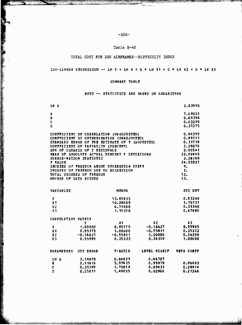
r^?s5P*?pppHS!!re!pw?sJ?^

cafe» 5J?PP|5^PP!^l|P»IISPBBPi«WBI«B69IPW5--

-104-

Table B-40

TOTAL COST FOR 100 A1RFRAMES—DIFFICULTY INDEX

LOG-LINEAR REGBESSION — LN I = LN A * B * LN XI ♦ C * LN X2 ♦ D * LH X3

SUMMART TABLE

NOTE -- STATISTICS ARE BASED ON LOGARITHMS

LN A 2.03995

A 7.69021 B 0.69396 C 0.63295 D 0.37275

COEFFICIENT OF CORRELATION (UNADJUSTED) 0.94399 COEFFICIENT OF DETERMINATION (UNADJUSTED) 0.89111 STANDARD ERROR OF THE ESTIMATE OF T (ADJUSTED) 0.31718 COEFFICIENT OF VARIATION (PERCENT) 2.28870 SUN OF SQUARES OF Y RESIDUALS 0.90541 HEAR OF ABSOLUTE ACTUAL E SRCENT Y DEVIATIONS 22.06449 DURBIN-WATSON STATISTIC 2.26368 F VALUE 24.55027 DEGREES OP FREEDCH ABOUT REGRESSION CURVE 9. DEGREES OF FREEDOM DUE TC RE3RESSION 3. TOTAL DEGREES OF FREEDOH 12. NUMBER OF DATA POINTS 13.

VARIABLES MEANS STD DEV

y 13.85835 0.83240 X1 10.28659 1.15731 X2 6.71468 0.39340 n 1. 15316 0.47490

CORRELATION MATRIX Y 11 12 13

Y 1.00000 0.85175 -0. 16627 0.55985 X1 0.85175 1.00000 -0. 55811 0.25332 X2 -0.16627 -0.55811 1. 00000 0.34359 X3 0.55985 0.25332 0. 34359 1.00000

PARAMETERS STD ERROR T-RATIO LEVEL SI3NIF BETA COEFF

LN A 3.14618 0.64839 0. 46707 B 0.11616 5.97415 0. 99979 0.96483 C 0.35199 1.79818 0. 89431 0.29914 D 0.25011 1.49035 0. 82968 0.21266

. ^- mm HHiMaMMi **~

«3"»s3W7*s—- - -* • - .1- -5;» ^i<vp<^wssMH|8i5wv|Pip>wt%{iW -: ";^S T

-105-

Table B-41

TOTAL COST FOR 100 AIRFRAMES—GROUP 1

LOG-LINEAR REGRESSION -- LN Y LN A ♦ B * LN XI

SUMMARY TABLE

NOTE — STATISTICS ARE BASEO ON LOGARITHMS

LN A

A B

COEFFICIENT OF CORRELATION (UNAOJUSTEOI COEFFICIENT OF DETERMINATION (UNAOJUSTEOI STANDARD ERROR OF THE ESTIMATE OF Y (ADJUSTED) COEFFICIENT OF VARIATION (PERCENT) SUM OF SQUARES OF Y RESIDUALS MEAN OF ABSOLUTE ACTUAL PERCENT Y DEVIATIONS DURBIN-WATSON STATISTIC F VALUE OEGRPES OF FREEDOM ABOUT REGRESSION CURVE DEGREES OF FREEDOM DUE TO REGRESSION TOTAL DEGREES OF FREEDOM NUMBER OF DATA POINTS

7.65322

21C7.%2486 0.58218

0.79480 0.63170 0.28995 2.20775 0.58848 17.82334 2.36527 12.00643 7. 1. 8. 9.

VARIABLES MEANS STO DEV

Y XI

13.13309 9.41259

0.44691 0.61012

PARAMETERS STO ERROR

LN A B

1.58443 0.16802

T-RATIO

4.83028 3.465C3

LEVEL SIGNIF

0.99810 0.9895?

BETA COEFF

0.79480

'■ i '.- ;I'-I ijj.iit-l-i iirli:"M»lfe^' , """

!>5WSf ' rw " '"* '** *~ : " ' ,:*"anra«*«*i

-106-

Table B-42

TOTAL COST FOR 100 AIRFRAMES—GROUP 2

LOG-LINEAR REGRESSION -- LN Y * LN A ♦ B * LN XI

SUMMARY TABLE

NOTE STATISTICS ARE BASEO ON LOGARITHMS

LN A 2.34432

COEFFICIENT OF CORRELATION (UNADJUSTED! COEFFICIENT OF DETERMINATION (UNADJUSTED) STANDARD ERROR OF THE ESTIMATE OF Y (ADJUSTED» COEFFICIENT OF VARIATION (PERCENT) SUM OF SQUARES OF Y RESIDUALS MEAN OF ABSOLUTE ACTUAL PERCENT Y DEVIATIONS DURBIN-WATSON STATISTIC F VALUE DEGREES OF FREEDOM ABOUT REGRESSION CURVE OEGREES OF FREEDOM DUE TO REGRESSION TOTAL OEGREES OF FREEDOM NUMBER OF DATA POINTS

10.42618 1.16458

0.96559 0.9323T 0.16053 1.15653 0.15463

11.91005 2,29148

82.71455 6. 1. 7. 8.

VARIABLES

Y XI

MEANS

13.83062 9.90594

STD DEV

0.57150 0.47385

PARAMETERS STD ERROR T-RATIO LEVEL SIGNIF BETA COEFF

LN A B

1.26973 0.12805

1.84632 9.09475

0.88563 0.99990 0.96559

_^

™W#j^.5l||^^

-107-

Table B-43

TOTAL COST FOR 100 AIRFRAMES—GROUP 3

LCG-LINFAR REGRESSION -- LN Y » LN A ♦ d * LN XI

SUMMARY TABLE

NCTE -- STATISTICS ARE öASEü CN LOGARITHMS

IN A

A B

COEFFICIENT COEFFICIENT STANDARO EP CCEFFICJ PNT

OF OF

ton OF

-.UM OF SCUARES

C0KKELAT10M I JNADJUSTEDJ OtTERMINATIÜN (UNADJUSTED) OF THE ESTIMATE OF Y UCJUSTEDI VARIATION (PERCENT) OF Y RESIDUALS

N'eAN cF ABSOLUTE ACTUAL PERCSNT Y DEVIATIONS DUBBIN-WATSON STATISTIC F VALUE DEGREES OF FREEDOM ABOUT REGRESSION CURVE DEGREES OF FREtüCM DUE TO REGRESSION TOTAL DEGREES OF FREEDOM NUMBER ff CATA POINTS

3.18*62

24.15820 0.96224

0.95118 0.9047<» 0.214©7 1.50569 0.18433

15.51110 2.49002

37.98869 4. 1. 5. 6.

VARIABLE?

Y XI

MtANS

14.25702 ll.iuc.9l

STO OEV

0.62208 0.61493

PARAMETERS STD ERROR

H A I. 7S858 J. 15612

T-RATIO

1.77063 o.16350

LEVEL SIGNIF

0.84e67 0.996*0

BETA COEF*

0.95118

u. - im-lir ■■)Mil in - — — — - ■"—-"*■-—

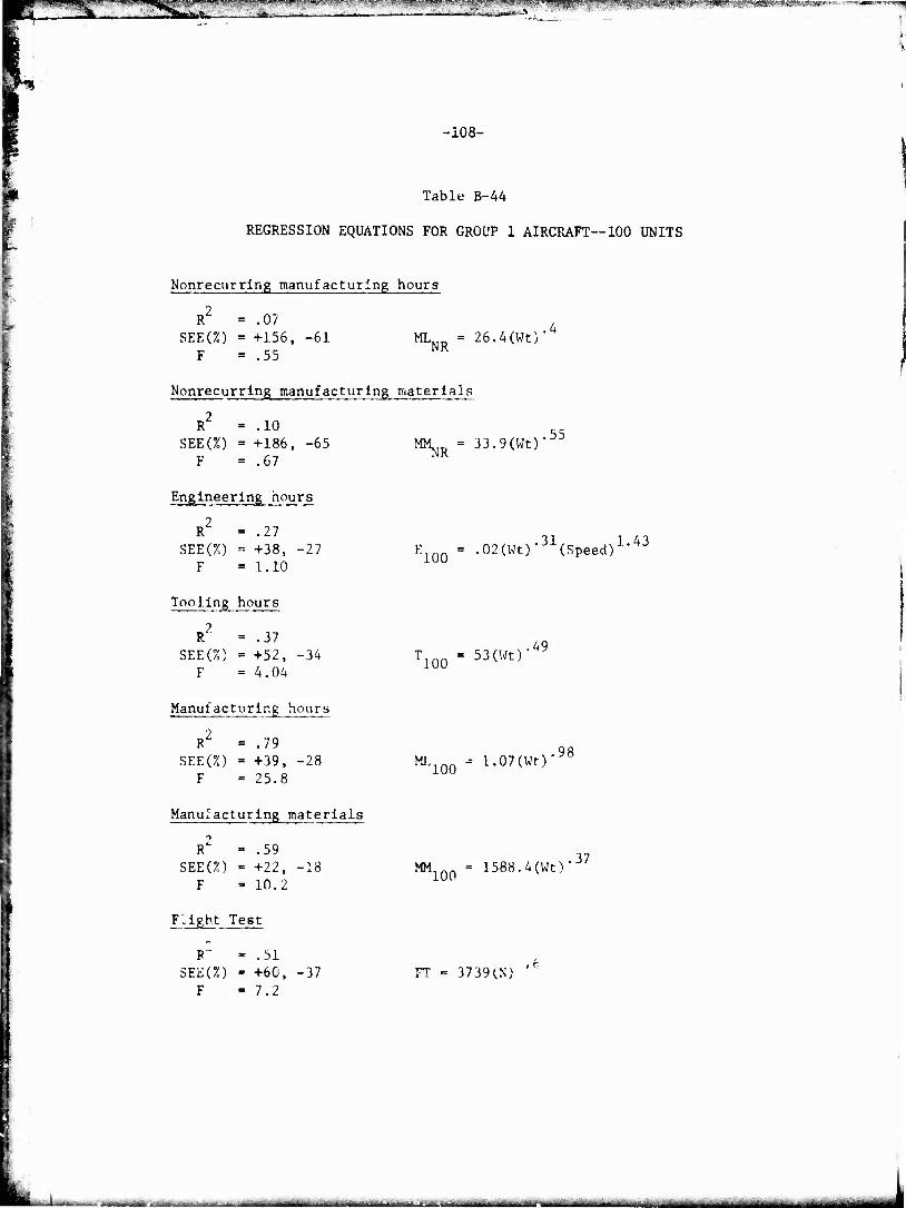
-108-

Table B-44

REGRESSION EQUATIONS FOR GROUP 1 AIRCRAFT—100 UNITS

Nonrecurring manufacturing hours

R = .07 SEE(%) = +156, -61

F = .55 MLNR = 26.4(Wt)"

4

Nonrecurring manufacturing materials

R = .10 SEE(%) = +186, -65

F = .67 MM^ = 33.9(Wt)

,55

Engineering hours

2 R = .27

SEE(%) « +38, -27 F -1.10

E100 = .02(Wt)-31(Speed)1,43

R = .37 SEE(%) = +52, -34

F = 4.04 T100 = 53(wt)

,49

Manufacturing hours

2 R = .79

SEE(%) = +39, -28 F = 25.8

ML100 -- 1.07(Wt) ,98

Manufacturing materlals

R2 - .59 SEE(%) = +22, -18

F = 10.2 MM = 1588.4(Wt)

.37

Flight Test

F" - .51 SEE(%) " +60, -37

F - 7.2 FT * 3739(N)

... .. ._^...-^_., Iiliiiirtiriiin - - ^lJMiilliriiiiiiiiiiiililiMlii«iiii«iii«

mmätt-.,*m-. t^.-,, ii...ir':i "''in.1! ;iI'../i^iitj -rr»Tf"'',A J "'

-109-

Table B-45

REGRESSION EQUATIONS FOR GROUP 2 AIRCRAFT--100 UNITS

Nonrecurring manufacturing houra

IT = .74 SEE(%) = +60, -37

F = 17.2 MLHD = .00069(Wt)

1.54

Nonrecurring__manufactur i ng materla 1

2 R = .62

SEE(%) = +68, -41 F =9.9

MM^ = .063(Wt) 1.30

Engi n eer 1 ng Jhou r s

R~ = .92 SEE(%) = +22, -18

F - 66.0 Eioo " -03(wt)

1.30

Tooling _hour_s

R2 = .59 SEEf%) = +45, -31

F = 8.6 T100 = !-54(Wt)

87

Manufacturing hours

R" = .83 SEE(%) = +30, -23

F =29.0 MLl0(J = .28(Wt)

1.12

Manuf ac tur i ng_ materials

R2 = .81 SEE(%) = +40, -29

F = 25.5 MM100 = .17(Wt)

1.38

Flijght Test

R" - .74 SF.E(%) = +52, -34

F = 7.2 FT = .098(WOKlo(N)"73

-—--- - - -■-"--" <~—. fc^ifrn in I 111—MMiIMM .III

gäu^i. - . . ^^r^^ - ., - -».-—~*WW -IT» J» SW*w»ww

-110-

Table B-46

REGRESSION EQUATIONS FOR GROUP 3 AIRCRAFT—100 UNITS

Nonrecurring manufacturing hours

R = .65 SEE(%) = +57, -36

F = 7.5 MLNR = .087(Wt)

.89

Nonrecurr'ing raanufacturing material

R*" = .40 SEE(%) = 114, -53

F =2.7 MMNR = .36(Wt)

,91

Engineering hours

2 R = .82

SEE(20 = +39, -28 F =18.6

Eioo = -095(wt) 1.02

Too] ing Jiours

R2 = .63 SEE(7„) = +40, -29

F = 6.7 Tioo " 9-14(Wt)

,64

Manufacturing hours

R2 = .92 SEE(%) = +20, -16

F - 46.9 ML100 = 1.16(Wt)

,90

Man uf ac turlng jna t e r t als

R2 = .81 SEE(%) = +54, -35

F ■ 17.1 MM100 = .079(Wt)

1.30

Flight Test

R2 = .39 SEE(%) - +156, -61

F * .95

„ ,,,„ s.74.,. 1.00 FT = .76(Wt) (N;

-ti IMinMM« ■■, n ..-...-. ma i - -- ----- ,.m

'~<WigW:XW~'; 'C'""^»K»«B

-Ill-

Table B-47

TOTAL COST—PROTOTYPE PROGRAMS

LOG-LINFAR REGRESSION — LN Y = LN A ♦ P * LN Kl ♦ C * LN X2

SUMMARY TABLE

NOTE — STATISTICS ARE BASED ON LOGARITHMS

LN A

t B r

CORRELATION I UNADJUSTED) DETERMINATION (UNADJUSTED) OF THE ESTIMATF PF Y (ADJUSTED) VARIATION (PFRCENT) OF Y RESIDUALS

PERCENT Y DEVIATIONS

COEFFICIENT OF COEFFICIENT OF STANDARD ERROR COEFFICIENT OF SUM OF SQUARES MEAN OF ABSOLUTE ACTUAL DURBIN-WATSON STATISTIC F VALUF DFGPEES OF FREEDOM ABOUT REGRESSION CURVF qEGREE? OF FREEDOM DUE TO REGRESSION TOTAL DEGREES OF FREEDOM NUMBFR OF DATA POINTS

7.01699

1115.42508 0.35300 0.98644

0.864 76 0.74782 0.30666 2.77849 0.65830 21.47897 2.46315

10.37881 7. 2. 9.

10.

VARIABLES MEANS STD DEV

Y XI X2

11.03711 9.72548 0.59506

0.53856 1.10835 0.33815

CORRELATION

Y XI X2

MATRIX Y

1.00000 0.61390 0.48732

XI 0.61390 1.00000

-0.18175

X2 0.48732

-0.18175 1.COOOO

PARAMETERS STD ERROR T-RATIO LEVEL SIGNIF BETA COEFF

LN A e r

0.96724 0.09379 0.30742

7.25462 3.76373 3.20879

0.99983 0.99296 0.98512

0.72648 0.61936

am mt urn mmlammimami

BL äk— ■!!j|Biil|)iBJWy^«^^ T^fÄgp^^^

A£. —Bit —-J=^- MIMl •'

-113-

Appendix C

USING ESTIMATING EQUATIONS

fi^c£ ^ IC

*«5* ^ ■4^

■^07» ,

'^Sfc

The preceding sections present a number of equations for estimating

both the major elements of cost—engineering hours, tooling hours, etc.—

and total cost as a function of such variables as weight, speed, and

time. Estimates resulting from those equations can vary enormously, de-

pending on the size and composition of the sample and on the explanatory

variables chosen. In view of such differences, it is natural to ask un-

der what circumstances those parametric equations can be relied on for

useful estimates.

There is no simple answer to that question. Disclaimers CP pp.

iii and 53 point out that the equations are intended for use only in

advanced planning activities when better information is not available.

Disclaimers of that type are often ignored, however, and parametric

models may be used in all phases of system acquisition. If, in fact,

an airframe model is suitable only for long-range planning studies, mis-

use is inevitable.

Another kind of misuse may also occur: the precision implied by a

mathematical model may inhibit the use of judgment. Logically, that at-

titude is indefensible because, as the following pages will show, oppon-

ents in the adversary procedure that characterizes system acquisitions

can find models to justify almost any set of numbers. Judgment is re-

quired in choosing a model representative of the aircraft whose cost is

to be estimated; and since no model can be completely representative,

judgment is required in interpreting the estimates obtained,

A previous Rand report, Cost-Estimating Relationships for Aircraft

Airfravnes, discusses statistical variations in predictions obtained

from models having a number of regression relationships. The intent of

this appendix is to show graphically the implications of changing the

composition of the sample and of choosing different independent vari-

ables.

G. S. Levenson et al., R-761-PR, December 1971, pp. 35-52,

Y^;<M***J*^. .■ , . .„.Jj- - ....... ._£, ,..|. | , ■ —

--—-—-—

«-*-■% -■■■■ ■■■■■ :■■ ..■■.-?MMte^fa^:-

-114-

By graphing the results of the equations, it is possible to examine

cost trends and to show visually where extrapolation will lead. The

relative importance of the individual cost elements should be appreci-

ated, and the advantage or disadvantages of highly aggregated models

compared with more detailed models should be explored. Only when an

estimating model is thoroughly understood can it be used effectively.

ENGINEERING HOURS

Figures C-l and C-2 show curves based on equations from preceding

sections that are repeated here for convenience:

1.

2.

3.

4.

6.

J100

'lOO

'100

'100

'100

"100

Equation

.00081 w-67V991r648

.00162 W751S1,175

.02344 V65V960

.02 W31S1*43

.03

.095 W

w1-3

1.02

Sample

24 aircraft—all types

24 aircraft—all types

9 newer aircraft—all types

Group 1 (9 small, slow aircraft)

Group 2 (8 small, fast aircraft)

Group 3 (6 large, slew aircraft)

where E.... = cumulative total engineering hours for 100 units

(thousands),

W = airframe unit weight (lb),

S = maximum speed at best altitude (kn),

T = number of quarters after 1942 in which first flight of a 3

pioduction aircraft occurs.

The curves suggest the problem encountered in using parametric es-

timating techniques. Estimates for a 100,000-lb aircraft with a maximum

speed of 550 kn and a production aircraft flight date of December 1975

range from 12 million to 23 million engineering hours. If the flight

date is advanced to the end of 1980, the range is 12 to 25 million.

Aircraft in each sample are identified in Table C-l. 3 The symbols W, S, and T are used throughout this appendix. In

subsequent equations, only symbols not previously used will be defined.

.. ^^-.-^.a^.: ..,_g. „„..■. . __ ,^c~a-.»;-:^.- —--.....- ...■■.._■»»»■.■-( r-tlfa»i- i-mti

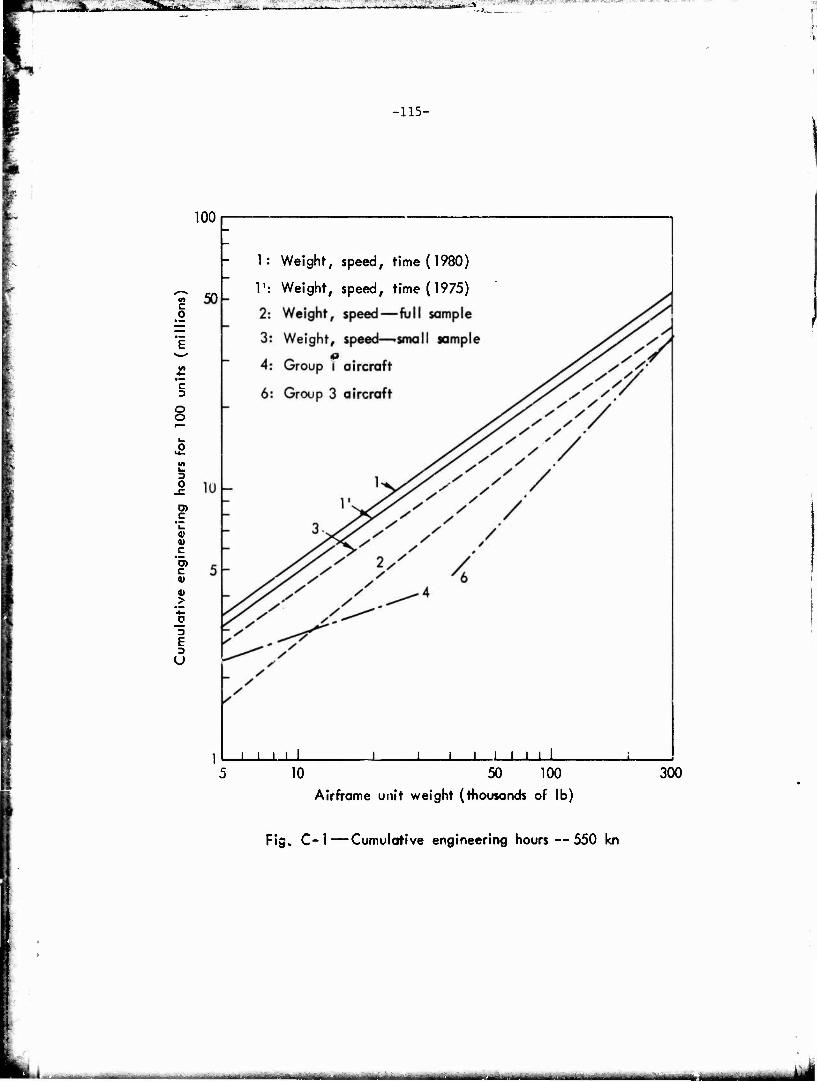
use «wviy^Trssg' ^::nvj u_ —-■-. ■■■■■■- ■ ir i ■- i- •-■■■■ ■a-:*itiY'\\"*rrrJUC*A j ;

i^jPSKfc-iv«?...™-

100

-115-

1: Weight, speed, time (1980)

1': Weight, speed, time (1975) c o

c

o o

3 o

D) C w V 4) C

'5) c

> ■*-

JO 3 E 3

1 I '''' J I I I I

10 50 100

Airframe unit weight (thousands of lb)

300

Fig. C-l—Cumulative engineering hours —550 kn

aük ^ -—j-

-116-

100

c 3

3 O

-C

O)

Im 0) V c

'rö c <u

>

3 E 3 u

50

/

HIII

1: Weight, speed, time (1980)

T: Weight, speed, time (1975)

2: Weight, speed—full sample

3; Weight, speed — smaM sample

5: Group 2 aircraft

J I I I I I I 10 50

Airframe unit weighi 'thousands of lb)

100

Fig. C-2 — Cumulative engineering hours — 1150 kn

*=■■■-■---■ - ■ ■ - - iTTifmirirtiJftr

■ äani jfcii». ;.^TT.«-.^'frrj«'^ !'■-'.-

-117-

For a 30,000-lb, 1150-kn aircraft, the range is about 15 to 23 million,

again a very substantial difference.

For the reasons discussed in Section III, we believe that the pre-

ferred equation for estimating engineering hours for future military

aircraft is Eq. 3. Howevar, as Table C-l shows, Eq, 3 badly overesti-

mates the engineering hours required for the A-5 and C-141 at 100 units,

and badly underestimates them for the B-58. We shall not attempt after-

the-fact rationalizations of these discrepancies, but in looking at es-

timates based on the equations shown throughout this report, it is es-

sential to keep one fact in mind: comparisons at the cost-element level

can be unreliable because of differences in definitions, in accounting

procedures, and in reporting practices among companies and among pro-

grams within the same company. Although engineering, tooling, manufac-

turing labor, etc., are carefully defined in the Contractor Cost Data

Report (CCDR), and prior to that in the Cost Information Report (CIR)

required of all contractors on military aircraft programs since 1967,

inconsistencies in the hours and dollars reported still exist. Indus-

trial engineering hours may be reported as engineering, tooling, or man-

ufacturing hours. Purchased engineering should be converted to engin-

eering hours, but it may be recorded as a material cost. Production

control may be categorized as either tooling or manufacturing. Certain

management functions are treated as indirect costs by one contractor

and as direct costs by another. And the differences are not trivial.

When queried on this subject, contractors stated that choice of one

category rather than another could perturb the results by as much as

20 percent.

TOOLING HOURS

The equation given in Section IV, p. 23, for cumulative tooling

hours is shown below as Eq. 1. Equations 2, 3, and 4 are taken from

Appendix B, pp. 108-110.

1 ""»• -—• ■-—■—-—- -—~ I—.—-..:—.„,,.- | - - -- ■-----.— - -^-^-,-J~,,. . .—,^~w i||aM||iflMg(||B|Bg|

R_ -at. '•ÜWfin'i"1ii1

-118-

Table C-l

Y-DEVIATIONS FOR SIX ENGINEERING-HOUR EQUATIONS ,a

m

Percent of Y-Deviation: Cumulative Engineering Hours at 100 Units

Aircraft Eq. 1 Eq. 2 Eq. 3 Eq. 4 Eq. 5 Eq. 6

A-3 -43 -65 -22 A-4 13 15 -25 A-5 -3 -8 -33 -26 A-6 19 32 -1 41

B-52 1 -23 0 B-58 45 39 27 15 RB-66 -49 -71 -13

C-130 43 43 33 C-133 13 7 -42 KC-135 -70 -80 -35 0-141 -25 -7 -37 4 C-5A 14 31 19 19

F-3 13 1 5 F-4 2 2 -23 10 F-6 16 12 -4 F-100 -19 -36 -44 F-102 20 17 14 F-104 -20 -29 17 F-105 3 -11 -11 F-106 -38 -50 -34 F-lll 9 24 11 4 F-14 -14 13 -2 12

T-38 37 46 17 18 T-39 -89 -43

Absolute mean 26 29 19 21 16 22

Percent deviation ■ Observed Y-Calculated Y Observed Y

... ——,. i. ,^__ l^^tlMIMMiiHa dmHK

-

-119-

Equatlon

1. Tinn = .472 W638S-4"

2' Tioo = 53w' 87

3. T100 - 1.54 W

4. T100-9.14W6

Sample

24 aircraft—all types

Group 1

Group 2

Group 3

where Tinn = cumulative total tooling hours at 100 units (thousands).

It will be noticed immediately that an important independent vari-

able—production rate—is missing; and since tooling hours are to some

extent a function of production r?te, the validity of the equations may

be questioned. The reasons why rate is not a statistically significant

variable were discussed earlier in this report. The problem is men-

tioned here because production rate helps to determine the point at

which all initial tooling hours have been incurred and that, in turn,

influences the slope of the cost-quantity curve. Where the planned

production rate is low—say, 4 aircraft per month—all nonrecurring

tooling hours will have been expended by the time about 20 aircraft

have been produced. The cumulative-tooling-hours curve will be rela-

tively flat thereafter, as only recurring tooling hours are incurred.

Curve A in Fig. C-3 is an example of that kind of program. Curves B

and C are examples of programs where the planned production rates were

higher, and nonrecurring tooling hours continued to be expended until

substantially more aircraft had been produced.

The stability in the relationship among the curves should be rea-

sonably gocd from 100 units on, and information from industry confirms

their utility. What about estimates for smaller quantities? The poten-

tii.1 for error is probably greater at 50 units than at 100, and greater

at 25 units than at 50, when the equations given above are used. The

sample is large enough, however, for a lot of the variability seen in

Fig. C-3 to wash out. Figure C-4 shows scaling curves plotted for four

production quantities. Ideally, all four would be parallel, but the

curves for 25 and 50 units are perceptibly steeper than the others.

They are not so different, however, that a crossover occurs within the

range of airframe unit weights in the sample.

ii \ liül^ilülifli - nur -■ - -- --■ - - - ■WUiHMAl MM ■MMflÜMiMlfeMIliihiMä

■»ja ■ ;--«r;m, ■.;:>.. ... ...■■V :77m*i»SK^- ■■■:: ■"■ --^IüB-'T-~ --iir'-i' I-"- -«T«rt> ' '' •"■•■•■ ■■ ■->*>■■***■-■■■' ^..„■fr.-.-.v^^j

-120-

40 50 60 80 100 Production quantity

200

Fig.C-3 — Cumulative tooling hours for three airframe programs

_^ - ummtam JBMM

-AÄL. .r*m***mmi:<i, fr«^.;»*»*'—* ,

-121-

10 50 100

Airframe unit weight (thousands of lb)

300

Fig. C-4 — Cumulative tooling hours for four production quantities — 550 kn

J^*_ ,.

------ . - . ., . . __ - - ----- -■—~ --itritiiii- «*■<■ -iiamitur --■■ ■

••'•^Ik IfciUii:». ii ■ " Yn] tan-—*

-122-

In addition to the question about production rate being used as an

explanatory variable, there is the ever-present question about the de-

sirability of working with smaller but more homogeneous samples, e.g.,

Groups 1, 2, and 3 mentioned earlier. Figure C-5 illustrates the re-

sults of one effort to use stratified samples. Curves 1 and 1' are

based on the entire sample; the other three curves are based on the

groups described under "Engineering Hours," above. The crossover of

Curves 2 and 3 says that Mach 2 aircraft require fewer tooling hours

than Mach .84 aircraft when the airframe unit weight is below 10,500

lb but more hours when the weight is greater. Such a conclusion is

illogical of course and must be rejected.

Curve 4 (Group 3 aircraft) lends some creHence to the notion that

cargo aircraft are enough different to be treated as a separate class,

i'hat can be done either by creating only a small sample of cargoes or

by incorporating a dummy variable in the estimating equation as shown

>-2low:

T100 = .522 W6V41DV ,322

where DV = dummy variable (DV = 1 for all types of aircraft except car-

go. DV = 2 for cargoes). The effect of both on Y-deviations is shown

below:

Percent of Y-Deviation

Aircraft Total Sample

Dummy Variable

Cargo Only

C-5 C-130 C-133 KC-135 C-141

-2 12

-15 16

-55

0 18

-11 2A

-45

4 -1

-36 24

-45 Absolute mean 20 20 22

By using a dummy variable, two estimates are improved, two are degraded,

one remains essentially the same, and the absolute mean is unchanged.

■■ -- - - - —"»■----— — '-jnffiiMfmnMiiii UBWM^aUMl

H- "*m ,. ■..■^■T-^rtiaL--^ ■ --. ^-' •■■•,- ■:■■**.;

•123-

I: All aircraft— 1150 kn

l1: Al! aircraft—550 kn

2: Group 1 aircraft

3: Group 2 aircraft

4 : Group 3 aircraft

1 I I I I I I ' ' i i i i i I 10 50 100

Airframe unit weight (thousands of lb)

300

Fig. C-5 — Cumulative tooling hours (100 units)

- "i -iir iim i MUÜMi ^Mnw>HBaiHkjMtotll*Jtf

m*&- «i&a^*. —*-— ir^Wtt* s

-124-

When cargo aircraft are treated as a separate sample, the results are

worse. Thus there is no persuasive reason to consider cargo aircraft

as a di.stir.Lt group insofar as tooling is concerned.

MANUFACTURING HOURS

Nonrecurring Hours

No potentially useful estimating equations for nonrecurring manu-

facturing hours were found except Eq. 1 below:

ML

ML

ML

NR

NR

NR

Equation Sample

000626 W,688S1,21 24 aircraft

00069 W1*54 Group 2

087 W89 Group 3

where ML NR nonrecurring manufacturing hours (thousands)

Figure C-6 shows curves based on Eq. 1 for two speeds—550 and 1150

kn—and curves for Groups 2 and 3 (the regression equation for Group 1 2

had such poor statistical properties, e.g., R = .07, that it is not

shown). The slope of the Group 2 curve is too steep to be credible; it

makes small airframes too cheap and large airframes too expensive.

Group 3 aircraft are again below the total sample, but that is because

all but one of thosi_ aircraft have speeds below 550 kn. The scaling

curves shown for the total sample appear to be representative of the

nonrecurring manufacturing hours in a normal airframe development pro-

gram.

Recurring Hours

In an aircraft production program, manufacturing labor is the

largest of the direct-cost elements; hence it is usually scrutinized more

carefully than the others. Unfortunately, the two best estimating

equations presented in Section V for manufacturing labor (Eqs. 1 and 2,

below) give rather different results, because one incorporates a time

variable and the other does not:

— ——^-^ - - imrtrUM —---■

mamtmm „I ii ■ri^rlliiniM.:;-i^*--'%

v 1

4 -125-

1: All aircraft—1150 kn

1': All aircraft—550 kn

2: Group 2 aircraft

3: Group 3 aircraft

J I l l i i '

10 50 100

A'rframe unit weight (thousands of ib)

300

Fig. C-6—Norirecurrirsg manfacturing hours

t*»-^^-** . ■ ■ ■■ ■ ■ -■ - - ■ - ■ - -■ ■•- ■ ■ ■ ■ -

■■Iv-I.»'f '-■-"'-:';g]'llilfi;- vrJ' "-"'■'"

-126-

Equation

1. M = .353 W79V423

2. Minn = .795 w-84V555T-535

98 3. M100=1.07W-

4. M100 = .28 V '

5. M100 = 1.16 WyU

Sample

24 aircraft—all types

24 aircraft—all types

Group 1

Group 2

Group 3

where Hlnn = cumulative recurring manufacturing hours at 100 units

(thousands).

The difference is shown in Figs. C-7 and C-8 in cumulative total

hours and in Figs. C-9 ar.d C-10 in unit hours per pound. (The. conver-

sion to unit hours assumed a cost-quantity curve slope of 77 percent.)

For a 50,000-lb airframe and a speed of 550 kn, Eq. 1 gives a value 46

percent higher than Eq. 2 when the time is 1975, and 58 percent higher

when the time is 1980. The differences are not so great for higher-

speed aircraft but they are sizable enough to be disturbing. Should

one assume that improvements in manufacturing techniques have reduced

hours to the extent indicated, or should one take a more conservative

view and argue that while some reduction has occurred, it is less dra-

matic than Eq. 2 suggests? One way to compare the two equations is to

ask which one does a netter job of estimating manufacturing hours for

recent aircraft. On the basis of the curves in Figs. C-7 to C-10,

we would expect the weight-speed equation to give consistently higher

estimates than the weight-speed-time equation. As shown by the Y-

deviations below, the difference for the three most recent aircraft—

the F-111, C-5, and F-14—ranges from 16 to 20 percent. In every case,

the equation with a time variable underestimates manufacturing hours.

In two cases, t;ie weight-speed equation overestimates hours. One might

be inclined to say that the truth lies somewhere in between, but the

Percent of Y-deviation

Aircraft Weight, Speed Weight, Speed, Time

F-111 C-5 F-14

-11 0

-4

5 17 16

»»-««^l^ii.^i«^^, ■*»»T1.,-. ,..» tmakamtmmn

;.s;' lyyKSwyy yx. ;.

i ■'• - "■■

-127-

100

=1 50h

5 8

3 O

-C

3 10 4- u £ 3

5 E CD 5 c

3 U V

0)

o "3 E 3 u

//y

'- AS' y/y y/y y /y syjy / y.y

//y / y A?

: // /^i

" // /?' V /' y^

// 1: Weight, speed

-// 2: Weight, speed, time (1975)

' 2': Weight, speed, time (1980)

3: Group 1 aircraft

5: Group 3 aircraft

... 1 J 1 1 1 1 1 1 1 1 ! 1 1 I 1

10 50 100 Airframe unit weight (thousands of lb)

300

H

Fig. C-7 — Cumulative recurring manufacturing hours—550 kn

- - - -

".»"V? • <;r>^**LÄi£■-■■■■•:■■&-.■ :-■■ - ^■■^ •:.■■--■■■>■ ;-■■■-■,:-^-..% v; ''ww™w»

-128-

100

50-

c o

c

8

3 O

O) c

3 u

>

_p 5 E U

10 -

5 >

-

-

' ///

^ // // r // / //

yf // /7 /' // /' //// ////

— / '// / ,y/ / /y - y //

- / S/

/" 7S/

'/ 1 : Weight, speed

- 2: Weight, speed, time (1975)

2': Weight, speed, time (1980)

4: Group 2 aircraft

.,. 1 1 II! i i i i i i i i

10 50

Airframe unit weight (thousands of lb)

100

Fig. C-8 — Cumulative recurring manufacturing hours — 1150 kn

IBM i -I'liT-mf

,/'!Ht - ' "iT!?ftllri>"i» gWa,.,-T. .. . ■•■v ^^-rwiimsiF-^q^^^^^^^^!^^

-129-

100

50 o o

c

-a c D O a

v Q.

3 o

c

o o <*• 3 C o E

c

10

1: Weight, speed

2- Weight, speed, time (1975)

2': Weight, speed, time (1980)

3: Group 1 aircraft

5: Group 3 aircraft

1 I I I I I I _L__J I I I I I

10 50 100

Airframe unit weight (thousands of lb)

300

Fig. C-9 — Unit recurring manufacturing hours per pound —550 kn

- llliÜMtMi

,'"'^-^Ä

-130-

100

50 -

8

3

C 3 O a

a

g 10

C

u o •*- 3 C O Z

c

1: Weigh*, speed

2: Weight, speed, time (1975)

2':Weight, speed, time ( 1980)

4: Group 2 aircraft

J I I I J_ .L

10 .0

Airframe unit weight (thousands of lb)

J L_L

KO

Fig. C-10—Unit recurring manufacturing hours per pound — 1150 kn

,J-,4—,^ .... :—,— ■ --■ .-,.^-,...

■Jk^ ■ ;v^>^, ■ --.. ■

•*"': "■;'.;:. .; ;;:-"' - ,;.:, \*™ '■y:jr^-v^"^xxrgij'y^"^sns^^

-131-

coefficient of the time variable (-.535) is such that a 7 percent de-

crease in hours is predicted between 1975 and 1980, and almost another

7 percent by 1985. Thus, in estimating manufacturing hours for future

aircraft, one must ask whether reductions of that magnitude are consis-

tent with investments in new capital equipment, developments in manu-

facturing techniques, new design practices, and new materials.

The decision on whether to use Eq. 1 (weight and speed) or Eq. 2

(weight, speed, and time) cannot be made without considering the impli-

cations for a closely related cot element; i.e., materials. Tf a time

variable is used for estimating manufacturing hours, a time variable

should be used for manufacturing materials as well. Reductions in labor

over time tend to be offset by increases in materials cost. That rela-

tionship is discussed below.

MANUFACTURING MATERIALS COST

The materials estimating equations in the main body of this report

were derived from 1973 costs. The constants below have been concerted

to 1975 dollars, using a composite index number of 1.273 derived by 4

means of a procedure described in a previous Rand report.

Nonrecurring Materials Cost

Equation

7? 1 72 1. MM = .0306 T' S

1 30 2. MM^ = .0802 W

3. MM^ = .^58 W91

Sample

24 aircraft—all types

Group 2

Group 3

where MM = nonrecurring materials cost (thousands of 1975 dollars).

Figure C-ll shows four scaling curves for nonrecurring materials

cost. (Group 1 is omitted because the regression equation had such

poor statistical properties.) Again we have the characteristics dis-

played by Groups 2 and 3 in virtually all cost elements—a very steep

slope for Group 2 aircraft and a lower cost for Group 3 because of their

H. G. Campbell, Aerospace Price Indexes, The Rand Corporation, R-568-PR, December 1970.

Ml m_m, yUH^^.^ ., ,=■ ^.^^^^^^^^ ... - -.s~-.^~^=.~-*.i~±~.*^*****Bmimimi*laä

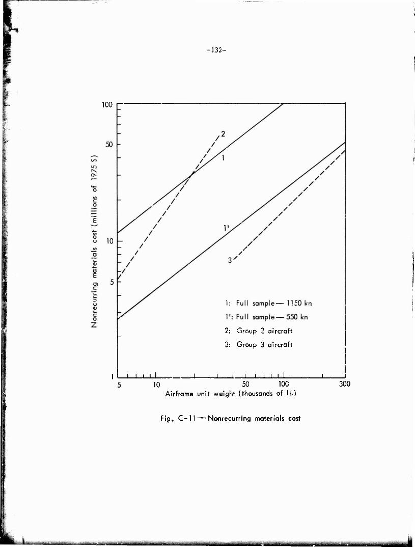
-132-

100

2: Group 2 aircraft

3: Group 3 aircraft

1 I I I I I ' L I I I I 10 50 100

Airframe unit weight (thousands of lb) 300

Fig. C-ll — Nonrecurring materials cost

-.-,.... ...,--■ ..-.JJ„_.^„—^^_—a,—-..-.^ iimniii

-133-

lower speed. Equation 1 is clearly preferable because the slope is rea-

sonable and the effect of different speeds can be taken into account.

Recurring Materials Cost

Equation

1. MM100 = .0316 W83V75V465

?.. MM100 = .0639 W88V867

3. MM = 1369 W406

4 MM 216 W 4. .iM100 .lib W

5. MM]00 = .101 Wi,:iU

Sample

24 aircraft—all types

24 aircraft—all types

Group 1

Group 2

Group 3

where MM1nr = cumulative recurring materials cost at 100 units (thous-

ands of 1975 dollars).

As in the case of manufacturing labor, two of the equations have

almost identical statistical values but give very different estimates.

Figures C-12 and C-13 show the difference in cumulative cost, and Figs.

C-14 and C-15 in unij cost per pound. For a 50,000-lb airframe and a

speed of 550 kn, Eq. 1 estimates a materials cost almost 40 percent

higher than Eq. 2 when T = 1975 and 67 percent higher when T = 1980.

The differences are not quite so great for higher-speed aircraft—28

percent for 1975 and 37 percent for 1980.

Theoretically, the idea of including a time variable is appealing

because a trend to higher-cost materials has been apparent for some

time. Practically, it is not clear that the use of a time variable

(at least in the way it is used here) will improve estimating accuracy.

A glance at the Y-deviations for the 10 most recent aircraft in the

sample ».Table C-2) does not show a pattern of increasing accuracy over

time.

Nor is any other pattern apparent. Except for the A-6, tiie two

equations underestimate the same aircraft and overestimate the same air-

craft. Both underestimate very small aircraft (the T-38 and T-39) and

very large aircraft (the C-5A). Both overestimate small aircraft (the

A-7) and large aircraft (the C-141). Both overestimate and underesti-

mate recent aircraft (the C-5 and F-14).

. _.-. ,..^^^-»-^_^^—...i....... —,-,....J.J,.^J..,... ,......„ ..„^.—,.^.^. —~.

-134-

1000

V»

10 50 100 Airframe unit weight (thousands of lb)

Fig. C-12 — Cumulative recurring materials cost—550 kn

■ mi, I, I,, - - - -11 TifMBliMfflni rtMMJMM^^

-135-

1000

1: Weight, speed, time (1980)

1': Weight, speed, time (1975)

2: Weight, speed

4: oroup 2 aircraft

10 50

Airframe unit weight (thousands of lb)

100

Fig. C- 13 — Cumulative recurring materials cost — 1150 kn

- _ -'■- —^ i in. r ,i, ■ ■ - -■- ■ _L ̂

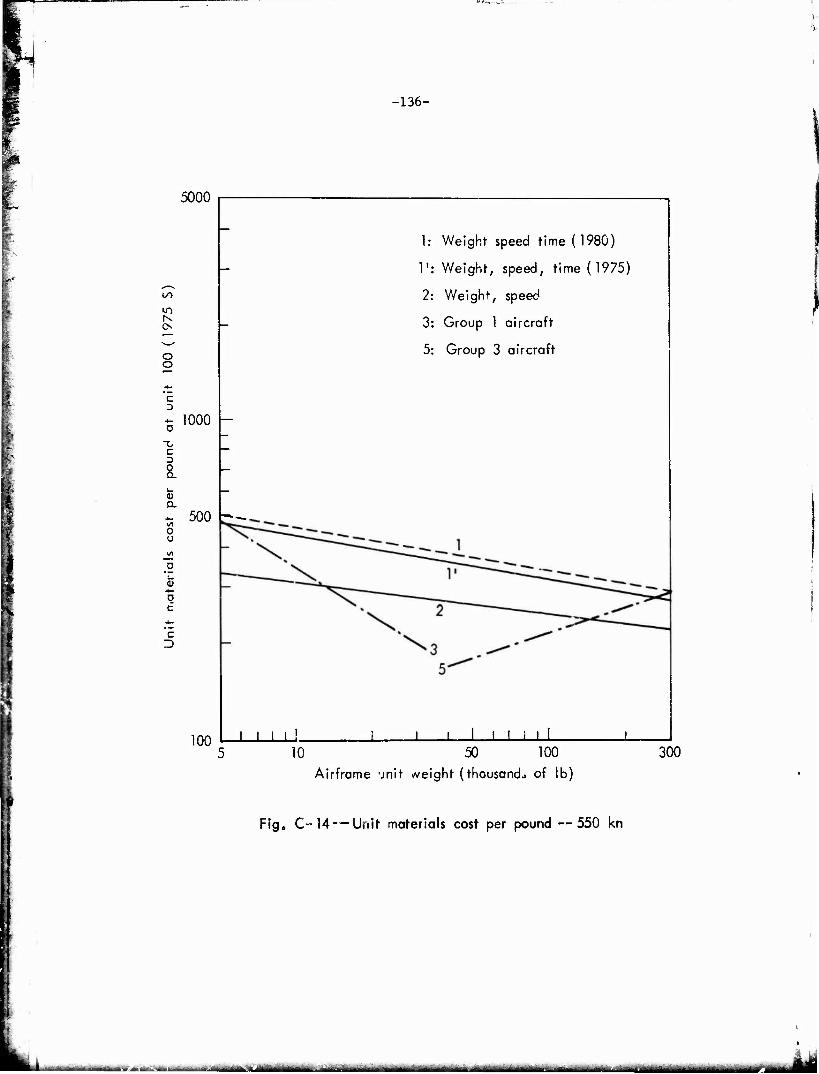
5000

-136-

K O

O O

1: Weight speed time (1980)

T: Weight, speed, time (1975)

2: Weight, speed

3: Group 1 aircraft

5: Group 3 aircraft

- 1000

C D

8. 0) a. - 500 VI 0 U

9

c

100 _L_L ±JJ. I I I I _L 10 50

Airframe jnit weight (thousand.; of lb)

300

Fig. C- 14™Unit materials cost per pound —550 kn

ühaiu -- -MlltlfMlBt»iMlilM1^n ■ —^■11 ■!■!■!

■137-

5000

O O

- 1000 -

C 3 0 a L. V Q.

O u

o £

500 -

100

1: Weight, speed, time ( 1980)

1': Weight, speed, time ( 1975)

2: Weight, speed

4: Group 2 aircraft

I I I I i J i i I i i i i 10 50 100

Airframe unit weight (thousands of lb)

300

Fig. C- 15 — Unit materials cost per pound — 1150 kn

Lfc,1 ■-"»■ i l-fmii^~~^-^~-~~-:'-^*,'*^**H***S!''m ■MtttijtiM »ü mn V i r inm ii ii um ill"

gra

-138-

Table C-2

PERCENT OF Y-DEVLATION FOR MATERIALS COST

Aircraft Weight, Speed Weight, Speed, Time Group 1, 2, or 3

A-5 2 6 -12 T-38 31 24 18 A-6 7 -4 19 T-39 22 7 22 F-4 15 15 21 C-141 -10 -24 -3 A-7 -7 -35 -6 F-lll 20 9 1 C-5 39 28 14 F-14 -7 -30 -11

Absolute mean 16 18 13

Range -10, +39 -35, +28 -12, +22

Since neither of the equations based on the full sample is really

satisfactory, one may be tempted to consider the results obtained for

the three subgroups. As shown by Table C-2, use of a more homogeneous

sample does reduce the range of Y-deviations markedly. However, for

Groups 2 and 3, the weight term has an exponent greater than one, and,

as seen in Figs. C-14 and C-15, the effect is to increase cost per

pound as airframe weight increases. This is contrary to experience,

so we do not believe that the curves for Groups 2 and 3 represent actual

trends. Problems with the data, and the influence of other variables

such as time and speed, can give spurious results with such small

samples.

Choice of the most appropriate estimating equation rests ultimately

on judgment. One consideration, mentioned previously, is that internal

consistency must be maintained in an overall airframe model. The same

variables should be used for both manufacturing labor and manufacturing

materials, i.e., either the time variable should be included for both

or for neither. The reason, of course, is that materials increase in

cost over time but labor hours are reduced; tfus they tend to offset

each other. One might assume that because of that balancing effect it

makes little difference which pair of equations is chosen. However, a

- ■ — - MMHaAM mmamtmmttmmggjjgjujgjgn

-139-

comparison of combined estimates made for airframes of aifferent sizes

and speeds shows that including the time variable consistently gives

results about 10 percent lower. Since experience teaches that the ten-

dency over time has been to underestimate aircraft costs, the better

choice on most occasions would be the equations that include only weight

and speed.

FLIGHT TEST COST

The equation for flight test costs in Section VII has been adjusted

by a factor of 1.177 to reflect the price-level increase since 1973:

1.

2.

3.

4.

FT

FT = 3739 N

FT

FT

Equation

153 W71S-59NJVL56

.76

.098 W1,16N'73

.76 W N

Sample

24 aircraft

Group 1

Group 2

Group 3

where FT = flight test cost (thousands of 1975 dollars)f

N = number of flight test vehicles,

DV = dummy variable (2 for cargo aircraft; 1 for all others).

Figure C-I6 shows three curves based on that equation when N = 5.

It is perhaps surprising that the curve for cargo aircraft is so much

lower than the curve for other military aircraft at the same speed.

Our data show, however, that flight test costs for the C-130, C-133,

KC-135, T-141, and C-5 are substantially lower, when compared on a

normalized basis, than the costs of the B-52 or the fighter-bombers.

Typically, flight test »josts for cargo aircraft are less than 2.5 per-

cent of total program cost for 100 aircraft, compared with 5 to 6 per-

cent for other aircraft. Mach 2 aircraft, as shown by curve 1, are

distinctly more expensive to test—their flight test costs are about

6 to 8 percent of total program cost for 100 aircraft.

TOTAL COST

It can be argued that inconsistencies in defining and accumulating

data for the individual cost elements make those data suspect, while

.».»j» jfc., -*•*»- ■ -^ ■--«.»—■ - —'—*——-"- -* --■■ —1_ _ -- - -^ ^^^^^riiBMMilililMM

500

-140-

c o

O U

5h 1: All aircraft—1150 kn

1': All aircraft—550 kn

1": Cargo aircraft—550 kn

2: Group 1 aircraft

3: Group 2 aircraft

4: Group 3 aircraft

1 I I I I I I 10

J I 1—i i ■ i ■ |

50 100 Airframe unit weight (thousands of lb)

Fig. C-16— Flight test cost (5 test aircraft)

300

■ *VMfMI , ' - - ■ ' -^ -vrrmMiniim«« - "■■-^—-*---'—"■-—

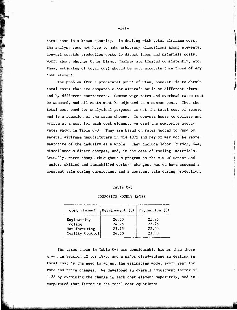
-141-

total cost is a known quantity. In dealing with total airframe cost,

the analyst does not have to make arbitrary allocations among elements,

convert outside production costs to direct labor and materials costs,

worry about whether Other Direct Charges are treated consistently, etc.

Thus, estimates of total cost should be mora accurate than those of any

cost element.

The problem from a procedural point of view, however, is to obtain

total costs that are comparable for aircraft built at different times

and by different contractors. Common wage rates and overhead rates must

be assumed, and all costs must be adjusted to a common year. Thus the

total cost used for analytical purposes is not the total cost cf record

and is a function of the rates chosen. To convert hours to dollars and

arrive at a cost for each cost element, we used the composite hourly

rates shown in Table C-3. They are based on rates quoted to Rand by

several airframe manufacturers in mid-1975 and may or may not be repre-

sentative of the industry as a whole. They include labor, burden, G&A,

miscellaneous direct charges, and, in the case of tooling, materials.

Actually, rates change throughout a program as the mix of senior and

junior, skilled and semiskilled workers changes, but we have assumed a

constant rate during development and a constant rate during production.

Table C-3

COMPOSITE HOURLY RATES

Cost Element Development ($) Production ($)

Engineering Tcoling Manufacturing Quality Control

26.50 24.25 23.75 :>4.50

21.75 22.75 22.00 23.00

The rates shown in Table C-3 are considerably higher than those

given in Section IX for 1973, and a major disadvantage in dealing in

total cost is the need to adjust the estimating model every year for

rate and price changes. We developed an overall adjustment factor of

1.28 by examining the change in each cost element separately, and in-

corporated that factor in the total cost equations:

<ua - maämmmtMi — ■ ■

-142-

Equation

7H 74 1. TC = 5.49 WS

2. TC = 2697 W

3. TC100 = 13.35 W1^6

4. TC100 = 30.92 WJ

Sample

24 aircraft—all types

Group 1

Group 2

Group 3

where TC _ = total cost for 100 units (thousands of 1975 dollars).

Figure C-17 shows two curves based on the total cost equation and

curves for each of the three aircraft subgroups. Again Group 2 has a

very steep slope, which makes small high-performance aircraft very cheap

and large high-performance aircraft very expensive. It depicts the

costs of Group 2 aircraft fairly well, but it is unsuitable for esti-

mating beyond the limits of the sample. Group 3 aircraft are again gen-

erally below the total sample, but the high cost of the C-5A relative

to other cargo aircraft influences the curve so that it intersects the

total-sample curve at about 300,000 lb.

The results obtained by using a data sample of total costs differ

very little from those obtained by summing the estimates of the individ-

ual cost elements. Figure C-18 shows total cost curves based on such

summations. Individual aircraft costs shown for reference purposes, it

must be remembered, are not the actual costs incurred by manufacturers.

The fact that estimates based on total cost are no better than

those based on a summation of estimates of each cost element is not sur-

prising. It has been suggested, however, that total-cost estimates are

more reliable than estimates of the individual elements because of com-

plementarities. For example, a lower-than-rwerage cost for manufactur-

ing labor may be offset by a higher-than-average cost for manufacturing

materials, etc. To test that hypothesis, we computed the percentage of

error contributed by each cost clement for all aircraft in the sample.

We estimated each cost element separately, using the equation described

Equations based on the full sample of 24 aircraft were used to estimate all individual cost elements except engineering. For engineer- ing, we used the full sample only for aircraft developed prior to 1958. Estimates of more recent aircr .ft were made using the equation based on a sample of 9 newer aircraft of all types.

ii*, _*^.k lfcla,J*''*i""" ' ■■■*■■—- -■mi- - iff"iTrililiiltHntllMl" i t-"i liiiTr'fiiirr r i ■ — --— --^- - ■■---■■ ■

-143-

10,000

5000

in C o

10 <D E o

o o

o u

S o

1000 -

500

100

-

-

yy 3

/ /

/ s X / /

- S/J7 4

1: All aircraft —1150 kn

I1: All aircraft—550 kn

7 2: Group 1 aircraft

3: Group 2 aircraft

4: Group 3 aircraft

i i i i i i i i i i i i i 1 i

10 50 100

Airframe unit weight (thousands of lb)

300

Fig. C-17 — Total airframe cost (100 units)

II iflllHiaiMani »lüT wmrnm *"»-■ -- ■ niifi • •!!■'• ' -T

10,000[

-144-

5000

c o

o o

o o

o

o o

1000

•T-39

1001—i i i I I

B: Speed =1150 kn, Time = 1975

C: Speed = 550 kn

D: Speed = 550kn, Time = 1975

• =<500kn 0 = 500- 750 kn A = >750kn

J 1 L_i_L 10 50 100

Airframe unit weight (thousands of lb)

Fig. C- 18 — Total airframe cost (10C units) based on summation of cost elements

300

*'■ '■- — i iri* ---■———*-■ —"~M i i i Miiiiiir mi- -'lüfliif- ''l- ■ .—»■ .,MJ.» —1, , ». , .^-„.a. „

-145-

in footnote 5 and, where necessary, converted to 1975 dollars. Table

C-4 shows the percentage? obtained. It appears that in 17 out of 24

cases, the sum of the errors is larger than any individual er^or. No

obvious complementarities are apparent between engineering ana manufac-

turing labor, manufacturing labor and materials, or tooling and manufac-

turing labor. In 6 oi the 24 cases, all elements have the same sign.

Thus, while complementarities undoubtedly exist in individual cases, no

pattern could be detected. That is clear is that manufacturing labor

is the greatest source of error, which is to be expected because it is

the most important cost element.

Table C-5 shows the percentage of total cost at unit 100 incurred

by each of the four major cost elements. We thought that certain sys-

tematic variations among percentages might occur, e.g., high-performance

aircraft might have a higher percentage of cost devoted to engineering

and large aircraft might have s higher percentage devoted to materials.

However, as Table C-5 makes evident, much of the variation is random.

Mach 2 aircraft tend to be above the mean in engineering and materials

and below the mean in manufacturing labor, but there are always axcep-

tions. Large aircraft are close to or below the mean in engineering,

close to the mean in l?.bor, and above the mean in materials. No gen-

eral observation about tooling is possible except that the hi',h-

performance aircraft tend to be at the low end of the ran^e.

What Table C-5 shows most forceably is the importance of manufac-

turing labor relative to the other cu'-r elements, and it becorres in-

creasingly important during the course of a prodjction program as fewer

engineering and tooling hours are incurred. Figure C-19 phows how the

percentage of total cost devoted to each cost element changes as uore

aircraft are produced. (The percentages were computed assuming a

30,000-lb, 1150-kn aircraft with a 20-aircraft flight test program.)

A good estimate of manufacturing labor reduces the possible margin

of error for an estimate of total cost. Parametric equations such as

those discussed here provide a good basis for an estimate, but when

other relevant information is available, it should be taken into con-

sideration. Since both industry and DoD agencies have long concentrated

on manufacturing-hours-per-pound curves, ther2 is more historical

■ ~-- •■itif'fr~*~-'**-iniiiihi *"■*****-"'■ ■ • ■-■-■—- WMOMMMMHaMUM

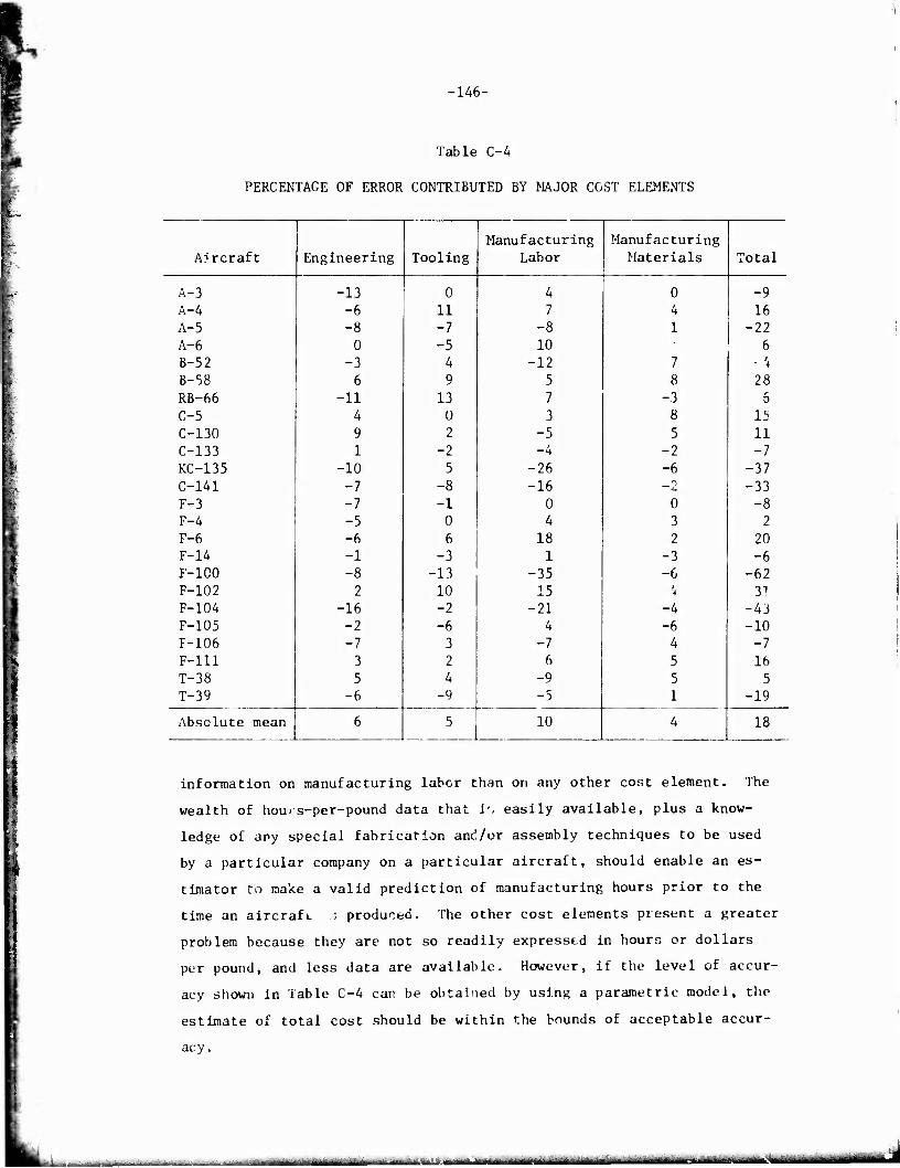
-146-

Table C-4

PERCENTAGE OF ERROR CONTRIBUTED BY MAJOR COST ELEMENTS

Manufacturing Manufacturing Aircraft Engineering Tooling Labor Materials Total

A-3 -13 0 4 0 -9 A-4 -6 11 7 4 16 A-5 -8 -7 -8 1 -22 A-6 0 -5 10 6 B-52 -3 4 -12 7 • '+

B-58 6 9 5 8 28 RB-66 -11 13 7 -3 6 C-5 4 0 3 8 15 C-130 9 2 -5 5 11 C-133 1 -2 -4 -2 -7 KC-135 -10 5 -26 -6 -37 C-141 -7 -8 -16 _0 -33 F-3 -7 -1 0 0 -8 F-4 -5 0 4 3 2 F-6 -6 6 18 2 20 F-14 -1 -3 1 -3 -6 F-100 -8 -13 -35 -6 -62 F-102 2 10 15 3i F-104 -16 -2 -21 -4 -43 F-105 -2 -6 4 -6 -10 F-106 -7 3 -7 4 -7 F-lll 3 2 6 5 16 T-38 5 4 -9 5 5 T-39 -6 -q -5 1 -19

Absolute mean 6 5 10 4 18

information on manufacturing labor than on any other cost element. The

wealth of hours-per-pound data that i', easily available, plus a know-

ledge of any special fabrication anc'/or assembly techniques to be used

by a particular company on a particular aircraft, should enable an es-

timator to make a valid prediction of manufacturing hours prior to the

time an aircraft ..; produced. The other cost elements present a greater

problem because they are not so readily expressed in hours or dollars

per pound, and less data are available. However, if the level of accur-

acy shown in Table C-4 can be obtained by using a parametric model, the

estimate of total cost should be within the bounds of acceptable accur-

acy.

üatiAfta^i. i IMBb>» . - - - - iM

-147-

Table C-5

PERCENTAGE OF TOTAL COST INCURRED LY INDIVIDUAL COST ELEMENTS

Engineering

% Aircraft

8 RB-66 9 A-3

12 B-52, KC-135, F-102 13 C-133, F-6, T- -39 14 A-4 15 F-3, F-106 19 C-5, C-130, C- -141 20 A-6 21 F-4, F-100 22 B-58, F-105 23 A-5, F-104, F- -111 28 F-14 31 T-38 18 Mean

Too I inq

% Ai?:craf t

12 A-5, F-105 13 A-6, C-5, F-14 14 F-lll 15 C-141, F-4 17 C-133 18 F-3 19 A-3, B-52, B-58, F-100 20 C-130, F-6, F-106, T-39 22 F-102 23 F-104, T-38 27 A-4 29 RB-66, KC-135 19 Mean

Manufacturing Labor Manufacturing Materials

I Aircraft % Aircraft

22 T-38 7 RB-66 28 F-104 10 F-6, F-105 29 B-58 11 C-133, F-3, F-102 30 F-106, F-lll 12 A-3, A-4 31 F-14 13 A-6, F-100 34 A-5 14 KC-135, F-104 36 B-52, F-4 16 C-130, T-38 37 F-100, A-4 17 F-4, F-14 38 C-i, F-102 18 B-58, F-106, T-39 39 C-141, KC-135, C-130 19 A-5, F-lll 40 T-39 20 B-52 42 F-3 22 C-141 43 A-6

F-6 F-105

25 C-5 46 15 Mean 4/ 48 RB-66 51 A-3 52 C-133 38 Mean

■■ri ii ni :~~~-~~.~ --■ .... MMH • ■

-148-

100

75

s o E E CD O i_ Q-

2 50 o

c

0)

25

Quality control

Flight test

Materials

Manufacturing labor

Tooling

Engineering

50 100

Aircraft product

150 200

Fig.C-19 — Percentage of cost devoted to major cost element*

u —i —-i——^ —iMilir i li IIIIMII P"irm . . „ m I—MMl^ltMäilMMtMii-itii __M^^mt^m—m, - --J

UNCLASSIFIED SEC'JRI "Y CLASSIFICATION Of T"!5 °ArC ,—li'n Dr'.a Fntr-erf)

REPORT DOCUMENTATION PAGE

F.-1693-1-P/^F/

2. GOVT ACCESSION NO

READ INSTRUCTION'S BFKOKE COMPLETING FORM

3. REC'PIENT'S CATALOG NUMBER

4. TITLE jmm>t f.kllll.)

Parametric Equations for Estimating Aircraft Airframe Costs»/ " —•—-

'," I T'PE InLer rim KjjjXt.K I

6. PERFORMING ORG. REPORT NUMBER

— ' ' II ll|FI j Y

Joseph P./£arge, Harry G.^ampbel 1fr

David Abates , f 75. 6- CON .R ACT OR GRAN' NLtl S E R(c)

DAHC15-71-C-322ff /

S. PERFORMING ORGANIZATION NAME AND ADDRESS

The Rand Corporation 1700 Main Street Santa Honica, Ca. 90406

10. PROGRAM ELEMENT. PROJECT, TASK AREA 6 WORK UNIT NUMBERS

11. CONTROLLING OfUCE NAME AND AODRESS

Asst Secretary of Defense (Program Analys Evaluation) DoD, Washington, D.C. 20301

W is andlüC .

■W. WliTUWI UM I E I

Feb mmm 1076 I

14. MONITORING AGENCY NAME ft ADDRESS^' dlllerenl tram Controlling Olllre) IS. SECURITY CLASS, (ol b

UNCLASSIFIED

15«. DECLASSlFI CATION/DOWNGRADING SCHEDULE

16. DISTRIBUTION STATEMENT (ol thin Report)

Approved for Public Release; Distribution Unlimited

17. DISTRIBUTION STATEMENT (ol the mbetract entered In Block 10. II dltterer.t from Report',

No Restrictions

16. SUPPLEMENTARY NOTES

19. KEY WOROS (Continue on reveree etde it neceeeary end Identity by block number)

Aircraft Cost Estimates Parametric. Equations

20 ABSTRACT (Continue ^TL revere* ei~'e II neceeemry enj Identity by block nutnber)

See reverse side

W) I JAW*»» 1473 f-OITIOW OF I MOV 65 IS OBSOLETE UNCLASSIFIED

a ,11 - - - ' -iir-" II I - -~ ******* ik

UNCLASSIFIED secuHiTY CLASSIFICATION OF THIS PAGerwh«> D«<* fini«r»d)

\ A set of generalized equations for estimating

development and production costs of aircraft

airframes on the basis of such characteristics

as aircraft weight and speed. (Extensive in-

vestigation has shown that these characteristics

explain cost variations better than any other

objective parameters.) Equations derived by

multiple-regression techniques are presented

for each of the major cost elements, for tctal

program cost, and for prototype development

costs. The report explains the derivation of

each equation and describes the treatment of

the data, the fitting of regression equations,

and selection of preferred equations. A

detailed numerical example is included

which applies to preferred equations and compares

the results to those obtained using several

sets of alternative equations. (JMD)

\

atmmsmtm