parametric designs and weight optimization using …
TRANSCRIPT

PARAMETRIC DESIGNS AND WEIGHT OPTIMIZATION USING DIRECT
AND INDIRECT AERO-STRUCTURE LOAD TRANSFER METHODS
A Thesis
Submitted to the Faculty
of
Purdue University
by
Viraj D. Gandhi
In Partial Fulfillment of the
Requirements for the Degree
of
Master of Science in Mechanical Engineering
August 2019
Purdue University
Indianapolis, Indiana

ii
THE PURDUE UNIVERSITY GRADUATE SCHOOL
STATEMENT OF COMMITTEE APPROVAL
Dr. Hamid Dalir, Co-chair
Department of Mechanical and Energy Engineering
Dr. John F. Dannenhoffer III, Co-chair
School of Mechanical and Aerospace Engineering
Dr. Carlos Larriba-Andaluz
Department of Mechanical and Energy Engineering
Approved by:
Dr. Jie Chen
Head of the Graduate Program

iii
“Building of science is depended on three pillars:
Discipline, Humbleness, and Regularity.
If any of the pillars is not strong enough, your building will collapse on your head.”
– High school Wall

iv
ACKNOWLEDGMENTS
I want to start with my advisors Dr. Hamid Dalir and Dr. John F. Dannenhoffer
III for their continuous motivation, support, and guidance throughout my research
work. I would also like to thank the member of the advisory committee, Dr. Carlos
Larriba-Andaluz, for his insightful feedback and encouragement which incented me
to widen my research from various perspectives.
I express special appreciation to Mr. Christian Aparicio and Mr. Julien Chaussee
for their valuable inputs toward various types of analysis of different parts; Ranu
Lavande for discussions related to creating API using C language and John Joe for
stimulating technical conversation as well as being my all-time competitor.
Additionally, I am grateful to all my colleagues at Advanced Composite Structures
Engineering Laboratory (ACSEL) for their support and keeping me sane; Udit Shah
for always motivating me (directly and indirectly) throughout my undergraduate and
graduate studies.
I would like to thank Mr. Jerry Mooney for his tireless efforts in reading this
thesis, catching typo’s and sentences which sounded like they were written at 4 A.M.
This work was funded by the CAPS project, which was funded under AFRL
Contract FA8050-14-C-2472: CAPS: Computational Aircraft Prototype Syntheses;
Dr. Dean Bryson is the Technical Monitor. I would like to acknowledge the discussions
with Dr. Nitin Bhagat, research engineer and AFRL contractor at the University of
Dayton Research Institute during the formulation of various parts of these aircraft
models.
Lastly, I would like to express my gratitude towards my parents who supported
me emotionally, financially and spiritually during my graduate study and in my life
in general. Special thanks to my brother for standing by me and having my back
during all the hardships.

v
TABLE OF CONTENTS
Page
LIST OF TABLES . . . . . . . . . . . . . . . . . . . . . . . . . . . . . . . . . . viii
LIST OF FIGURES . . . . . . . . . . . . . . . . . . . . . . . . . . . . . . . . . ix
SYMBOLS . . . . . . . . . . . . . . . . . . . . . . . . . . . . . . . . . . . . . . xi
ABBREVIATIONS . . . . . . . . . . . . . . . . . . . . . . . . . . . . . . . . . . xii
NOMENCLATURE . . . . . . . . . . . . . . . . . . . . . . . . . . . . . . . . . xiii
ABSTRACT . . . . . . . . . . . . . . . . . . . . . . . . . . . . . . . . . . . . . xiv
1 INTRODUCTION . . . . . . . . . . . . . . . . . . . . . . . . . . . . . . . . 1
1.1 Aerodynamic Load Transfer on The Structure . . . . . . . . . . . . . . 1
1.2 Parametric Design and Optimization . . . . . . . . . . . . . . . . . . . 2
1.3 Motivation . . . . . . . . . . . . . . . . . . . . . . . . . . . . . . . . . . 3
2 REVIEW OF LITERATURE . . . . . . . . . . . . . . . . . . . . . . . . . . 5
2.1 Fluid Analysis . . . . . . . . . . . . . . . . . . . . . . . . . . . . . . . . 5
2.1.1 Boundary Layer Thickness . . . . . . . . . . . . . . . . . . . . . 5
2.1.2 Governing Equations . . . . . . . . . . . . . . . . . . . . . . . . 6
2.1.3 Turbulence Modeling . . . . . . . . . . . . . . . . . . . . . . . . 7
2.1.4 Fluid-Structure Interaction . . . . . . . . . . . . . . . . . . . . . 11
2.1.5 Prediction of Lift . . . . . . . . . . . . . . . . . . . . . . . . . . 14
2.2 Structural Analysis . . . . . . . . . . . . . . . . . . . . . . . . . . . . . 15
2.2.1 Multipoint Constraint Element . . . . . . . . . . . . . . . . . . 15
2.2.2 Nastran File Structure . . . . . . . . . . . . . . . . . . . . . . . 17
2.2.3 Nastran Cards . . . . . . . . . . . . . . . . . . . . . . . . . . . . 19
2.2.4 Optimization Solver . . . . . . . . . . . . . . . . . . . . . . . . 21
2.3 Parametric Designs . . . . . . . . . . . . . . . . . . . . . . . . . . . . . 21
2.3.1 Engineering SketchPad . . . . . . . . . . . . . . . . . . . . . . . 22

vi
Page
2.3.2 Naca 4-digit Airfoil Generation . . . . . . . . . . . . . . . . . . 22
2.3.3 Attributes in ESP . . . . . . . . . . . . . . . . . . . . . . . . . . 25
2.3.4 Buildup Element Model . . . . . . . . . . . . . . . . . . . . . . 26
3 COMPARISON OF DIRECT AND INDIRECT AERO-STRUCTURE LOADTRANSFER METHOD . . . . . . . . . . . . . . . . . . . . . . . . . . . . . 27
3.1 Fluid Analysis . . . . . . . . . . . . . . . . . . . . . . . . . . . . . . . . 27
3.1.1 Geometry of Wing . . . . . . . . . . . . . . . . . . . . . . . . . 27
3.1.2 Fluid Domain and Mesh . . . . . . . . . . . . . . . . . . . . . . 27
3.1.3 Boundary Conditions . . . . . . . . . . . . . . . . . . . . . . . . 31
3.1.4 Convergence Check and Comparison . . . . . . . . . . . . . . . 32
3.2 Structural Analysis . . . . . . . . . . . . . . . . . . . . . . . . . . . . . 34
3.2.1 Geometry . . . . . . . . . . . . . . . . . . . . . . . . . . . . . . 34
3.2.2 Mesh . . . . . . . . . . . . . . . . . . . . . . . . . . . . . . . . . 35
3.2.3 Material and Properties . . . . . . . . . . . . . . . . . . . . . . 35
3.2.4 Loads on The Wing . . . . . . . . . . . . . . . . . . . . . . . . . 36
3.3 Load Transfer Using FSI . . . . . . . . . . . . . . . . . . . . . . . . . . 36
3.4 Load Transfer Using Stick Model . . . . . . . . . . . . . . . . . . . . . 37
3.5 Result and Comparison . . . . . . . . . . . . . . . . . . . . . . . . . . . 43
3.6 Conclusion . . . . . . . . . . . . . . . . . . . . . . . . . . . . . . . . . . 44
4 WEIGHT OPTIMIZATION OF WING USING INDIRECT LOAD TRANS-FER METHOD . . . . . . . . . . . . . . . . . . . . . . . . . . . . . . . . . . 50
4.1 User Inputs . . . . . . . . . . . . . . . . . . . . . . . . . . . . . . . . . 50
4.2 Geometry Script . . . . . . . . . . . . . . . . . . . . . . . . . . . . . . 51
4.3 Analysis Setup . . . . . . . . . . . . . . . . . . . . . . . . . . . . . . . 54
4.3.1 Static Structural Failure Mode . . . . . . . . . . . . . . . . . . . 55
4.3.2 Buckling Failure Mode . . . . . . . . . . . . . . . . . . . . . . . 57
4.4 Results . . . . . . . . . . . . . . . . . . . . . . . . . . . . . . . . . . . . 59
4.5 Conclusion . . . . . . . . . . . . . . . . . . . . . . . . . . . . . . . . . . 61

vii
Page
5 PARAMETRIC DESIGN OF AIRCRAFT USING ENGINEERING SKETCH-PAD (ESP) . . . . . . . . . . . . . . . . . . . . . . . . . . . . . . . . . . . . 64
5.1 Military Aircraft Prototype Syntheses . . . . . . . . . . . . . . . . . . . 64
6 CONCLUSIONS AND FUTURE WORK . . . . . . . . . . . . . . . . . . . . 72
6.1 Conclusion . . . . . . . . . . . . . . . . . . . . . . . . . . . . . . . . . . 72
6.2 Future Scope . . . . . . . . . . . . . . . . . . . . . . . . . . . . . . . . 72
REFERENCES . . . . . . . . . . . . . . . . . . . . . . . . . . . . . . . . . . . . 74

viii
LIST OF TABLES
Table Page
3.1 Convergence Check (Growth Rate Change) . . . . . . . . . . . . . . . . . . 33
3.2 Convergence Check (Boundary Layer Height Change) . . . . . . . . . . . . 33
3.3 Comparison With XFLR5 . . . . . . . . . . . . . . . . . . . . . . . . . . . 33
3.4 Total Load Data . . . . . . . . . . . . . . . . . . . . . . . . . . . . . . . . 40
3.5 Difference in Maximum Deformation . . . . . . . . . . . . . . . . . . . . . 44
4.1 Design Parameters of Wing and Panels . . . . . . . . . . . . . . . . . . . . 53
4.2 Results of Optimized Geometry . . . . . . . . . . . . . . . . . . . . . . . . 60
5.1 Design Parameters . . . . . . . . . . . . . . . . . . . . . . . . . . . . . . . 67
5.2 Design Parameters for Figure 5.8 . . . . . . . . . . . . . . . . . . . . . . . 69

ix
LIST OF FIGURES
Figure Page
2.1 Boundary Layer Thickness . . . . . . . . . . . . . . . . . . . . . . . . . . . 6
2.2 Transferring Node Data to Face Data . . . . . . . . . . . . . . . . . . . . . 12
2.3 General Grid Interface Mapping . . . . . . . . . . . . . . . . . . . . . . . . 14
2.4 Load Transfer to CG . . . . . . . . . . . . . . . . . . . . . . . . . . . . . . 16
2.5 Force and Moment Distribution . . . . . . . . . . . . . . . . . . . . . . . . 17
2.6 Nastran File Structure . . . . . . . . . . . . . . . . . . . . . . . . . . . . . 18
2.7 Airfoil Nomenclature . . . . . . . . . . . . . . . . . . . . . . . . . . . . . . 23
2.8 Points Distribution . . . . . . . . . . . . . . . . . . . . . . . . . . . . . . . 26
3.1 Wing Geometry . . . . . . . . . . . . . . . . . . . . . . . . . . . . . . . . . 28
3.2 Fluid Domain Surrounding Wing . . . . . . . . . . . . . . . . . . . . . . . 29
3.3 Mesh Around the Airfoil . . . . . . . . . . . . . . . . . . . . . . . . . . . . 30
3.4 Mesh Near Surface of Wing . . . . . . . . . . . . . . . . . . . . . . . . . . 30
3.5 Boundary Conditions of Fluid Domain . . . . . . . . . . . . . . . . . . . . 31
3.6 Pressure Contours on The Wing and XY Plane at Z = 5m . . . . . . . . . 32
3.7 Wing With Internal Structure . . . . . . . . . . . . . . . . . . . . . . . . . 34
3.8 Structural Mesh Near Leading Edge . . . . . . . . . . . . . . . . . . . . . . 35
3.9 Load Transfer Using FSI . . . . . . . . . . . . . . . . . . . . . . . . . . . . 37
3.10 Pressure Center of Sections . . . . . . . . . . . . . . . . . . . . . . . . . . 39
3.11 Load Transfer from Pressure Center to Geometric Center . . . . . . . . . . 40
3.12 Shear-Moment-Torque . . . . . . . . . . . . . . . . . . . . . . . . . . . . . 42
3.13 RBE3 on Edge of Rib . . . . . . . . . . . . . . . . . . . . . . . . . . . . . 43
3.14 Load Applied Using Discretized Load Transfer Method . . . . . . . . . . . 44
3.15 Structural Deformation Using Distributed Load Transfer Method (alfa = 7) 45
3.16 Structural Deformation Using Discretized Load Transfer Method (alfa = 7) 46

x
Figure Page
3.17 Deformation vs Span at Leading Edge (Alfa = 7) . . . . . . . . . . . . . . 47
3.18 Deformation vs Span at Trailing Edge (Alfa = 7) . . . . . . . . . . . . . . 48
3.19 Deformation vs Span (Alfa = 4) . . . . . . . . . . . . . . . . . . . . . . . . 48
3.20 Deformation vs Span (Alfa = 0) . . . . . . . . . . . . . . . . . . . . . . . . 49
4.1 Loadcase CSV File . . . . . . . . . . . . . . . . . . . . . . . . . . . . . . . 52
4.2 Rib Attributions . . . . . . . . . . . . . . . . . . . . . . . . . . . . . . . . 54
4.3 Example of Panel Attribution . . . . . . . . . . . . . . . . . . . . . . . . . 55
4.4 Flowchart for Geometry Script . . . . . . . . . . . . . . . . . . . . . . . . . 56
4.5 RBE3 Connection . . . . . . . . . . . . . . . . . . . . . . . . . . . . . . . . 57
4.6 Edge Attributions of Unstiffened and Stiffened Panel . . . . . . . . . . . . 58
4.7 Flowchart for Analysis Process . . . . . . . . . . . . . . . . . . . . . . . . 62
4.8 Optimized Upper Surface . . . . . . . . . . . . . . . . . . . . . . . . . . . 63
4.9 Optimized Lower Surface . . . . . . . . . . . . . . . . . . . . . . . . . . . . 63
5.1 ESP Tree Structure to Generate a Military Fighter Aircraft . . . . . . . . 64
5.2 Middle Section of Aircraft . . . . . . . . . . . . . . . . . . . . . . . . . . . 65
5.3 Solid OML . . . . . . . . . . . . . . . . . . . . . . . . . . . . . . . . . . . 66
5.4 Waffle for Vertical Stabilizer . . . . . . . . . . . . . . . . . . . . . . . . . . 67
5.5 Waffle Without Vertical Stabilizer . . . . . . . . . . . . . . . . . . . . . . . 69
5.6 Continuous Waffle . . . . . . . . . . . . . . . . . . . . . . . . . . . . . . . 70
5.7 Internal Structure . . . . . . . . . . . . . . . . . . . . . . . . . . . . . . . . 70
5.8 Aircraft with Different Configurations . . . . . . . . . . . . . . . . . . . . . 71

xi
SYMBOLS
Cf Empirical constant
τw Shear stress rate
Uf Frictional velocity
H Boundary layer thickness
y+ Height of first cell near wall
Γ Effective diffusivity
k Turbulence Kinetic Energy
w Specific dissipation rate
Cl Lift coefficient
m mass
v velocity

xii
ABBREVIATIONS
attr Attributes
CFD Computational Fluid Dynamics
FSI Fluid-Structure Interaction
VLM Vortex Lattice Method
MPC Multipoint Constraint
CG Center of Gravity
CSG Constructive Solid Geometry
BRep Boundary Representation
MDAO Multidisciplinary Design, Analysis and Optimization
EGADS Engineering Geometry Aircraft Design System
ESP Engineering Sketch Pad
BEM Built Up Element Model
OpenCSM Open-source Constructive Solid Modeler
DM DesignModeler
SMT Shear-Moment-Torque
OML Outer Mold Layer
NSSE Navier-Stoke System of Equations
RANS Reynolds Average Navier-Stoke
DNS Direct Numerical Solution
Tx Translation in X axis
Rx Rotation in X axis
GGI General Grid Interface
CAPS Computational Aircraft Prototype Syntheses
UDP User-Defined Primitive

xiii
NOMENCLATURE
Alfa Angle of attack
.bdf Nastran analysis deck
Chord line a straight line joining leading edge and trailing edge in airfoil
Camber line halfway line between upper and lower surface
Camber (local) Distance between camber line and chord line
xiv
ABSTRACT
Gandhi, Viraj D. M.S.M.E., Purdue University, August 2019. Parametric Designsand Weight Optimization Using Direct and Indirect Aero-Structure Load TransferMethods. Major Professors: Dr. Hamid Dalir and Dr. John F. Dannenhoffer III.
Within the aerospace design, analysis and optimization community, there is an
increasing demand to finalize the preliminary design phase of the wing as quickly as
possible without losing much on accuracy. This includes rapid generation of designs,
an early adaption of higher fidelity models and automation in structural analysis of
the internal structure of the wing. To perform the structural analysis, the aerody-
namic load can be transferred to the wing using many different methods. Generally,
for preliminary analysis, indirect load transfer method is used and for detailed anal-
ysis, direct load transfer method is used. For the indirect load transfer method,
load is discretized using shear-moment-torque (SMT) curve and applied to ribs of
the wing. For the direct load transfer method, the load is distributed using one-
way Fluid-Structure Interaction (FSI) and applied to the skin of the wing. In this
research, structural analysis is performed using both methods and the nodal dis-
placement is compared. Further, to optimize the internal structure, iterative changes
are made in the number of structural members. To accommodate these changes in
geometry as quickly as possible, the parametric design method is used through En-
gineering SketchPad (ESP). ESP can also provide attributions the geometric feature
and generate multi-fidelity models consistently. ESP can generate the Nastran mesh
file (.bdf) with the nodes and the elements grouped according to their geometric at-
tributes. In this research, utilizing the attributions and consistency in multi-fidelity
models an API is created between ESP and Nastran to automatize the multi-fidelity
structural optimization. This API generates the design with appropriate parameters

xv
and mesh file using ESP. Through the attribution in the mesh file, the API works as
a pre-processor to apply material properties, boundary condition, and optimization
parameters. The API sends the mesh file to Nastran and reads the results file to
iterate the number of the structural member in design. The result file is also used to
transfer the nodal deformation from lower-order fidelity structural models onto the
higher-order ones to have multi-fidelity optimization. Here, static structural opti-
mization on the whole wing serves as lower fidelity model and buckling optimization
on each stiffened panel serves as higher fidelity model. To further extend this idea, a
parametric model of the whole aircraft is also created.

1
1. INTRODUCTION
In a broad way, the objective of this research is to create a tool that can optimize the
structural aspects of the preliminary design of the whole aircraft by executing a single
file. Here, as the optimization needs to be done for the preliminary design phase, it
should be as quickly as possible without losing much on accuracy. To achieve the goal,
the project is divided into three main steps. 1) Check the reliability of discretized
load transfer method; 2) Optimize the internal structure of the wing as a proof of
concept; 3) Expand the 2nd step for the whole aircraft.
1.1 Aerodynamic Load Transfer on The Structure
For the purpose of structural analysis, there are many ways to transfer the aero-
dynamic load to structure which is mainly divided into two categories; direct and
indirect load transfer. Selection of the method depends upon design phase, geometry
and amount of accuracy required. Indirect method can be considered as a discretized
load transfer method because the loads are applied discretely on the structural mem-
bers. While the direct method can be considered as a distributed load transfer method
as loads are applied on each node of the skin.
For the preliminary design phase, the indirect load transfer method is generally
used. In this method, the aerodynamic geometry is divided into several sections
and the loads on each section is concentrated on a single node. By connecting the
nodes, a stick model representation is created. Aerodynamics team gives this data to
structural analysis team and then the load is redistributed on the structural members.
All these conversions might result in compromising the localized accuracy.
For distributed load transfer, Fluid Structure Interaction (FSI) technique is used.
There are two main techniques of coupling fluid with the structure, fully coupled and

2
another is partially coupled. In the fully coupled analysis, equations of structural
analysis are incorporated into the fluid analysis and behavior of the whole system
is calculated simultaneously. This method is generally tailored to the problem and
not typically used in industry even for the final design phase. In the partially cou-
pled analysis, structural analysis lags behind the fluid analysis. To perform partially
coupled analysis, the first step is to perform fluid analysis. Then the contact surface
between the fluid domain and the structure is identified. The required data is then
transferred to the structural surface from the fluid domain using different algorithms
(algorithm depends on the type of data being transferred). The structural analysis is
performed to calculate the deformation of nodes. In one-way FSI, the analysis ends
here but in two-way FSI, the deformation from the structural analysis is transferred
to the fluid domain. The mesh of fluid domain is morphed to accommodate the
structural displacement and the fluid analysis is performed again. For steady state
case, and the loop continues till equilibrium is achieved. For unsteady state case, it
continuous till given loop iterations.
In this research, the structural response of the wing is compared between stick-
model method and one-way FSI method. In both methods, the underlying assumption
is that the wing is a semi-rigid structure. Which means that the structure is rigid till
all the load is applied and then it deforms [1].
1.2 Parametric Design and Optimization
In the design, analysis, and optimization of aerospace vehicles and structures, it is
absolutely crucial to generate the geometry fast and in a robust way [2]. For a given
aerodynamic geometry, the number of structural solutions to support the design are
unlimited. However, there is only one solution which could lead to the minimum
weight for the structure. To realize this, a single common consistent parametric
description of the design against different disciplines is necessary.

3
In Multi-Disciplinary Analysis and Optimization (MDAO) environments, it is a
common practice to import the models from manufacturing design tools with usually
IGES and STEP extensions. Although these structural parts and components are
intended to be ultimately manufactured, the use of these extensions will create static
(non-parametric) geometry models. These models cannot be used to optimize discon-
tinuous design variables such as the number of stiffeners. Also to create a Boundary
Representation (BRep), the models should be closed watertight which is extremely
difficult due to the lack of a complete solid modeling geometry kernel to deal with
the topology data if any [3].
A web-browser based integrated software referred to as the Engineering Sketch
Pad (ESP) [3], is used here which completely resolves the issues mentioned above.
ESP is parametric design software which creates a design using CSM script file. The
script file is in ASCII format and can be read using any text editors. The ESP can be
coupled with many analysis software using its ability to attribute geometric feature.
In this research, the ESP is used to generate parametric designs and to generate
Nastran analysis deck file. This deck file contains only mesh data and related attri-
butions. This file is then edited and sent to Nastran to perform the required analysis.
The generation of CSM script and communication between ESP and Nastran is car-
ried out by in-house C program API. User needs to provide aerodynamic parameters
and structural parameters in a comma separated variable (CSV) file. User also need
to provide loadcases for which the geometry needs to be optimized in another CSV
file. After providing the inputs, the user needs to execute one file to get the optimized
parameters.
1.3 Motivation
The time required to finalize the internal structure of aircraft is directly impacted
by the time require to make repetitive changes in design and preprocessing. The
changes in designs are usually the number of structural members. Unlike thickness,

4
these geometric features cannot be incorporated into the stiffness matrix without
physical presence. Also, if multi-disciplinary and/or multi-fidelity analysis needs to
be performed, the regeneration of different models with consistent parameters is fal-
lible and time-consuming. Thus, reduction in complexity between different models
and automatization of regeneration of design is necessary. For the preprocessing, gen-
erally after iterative changes, similar mesh parameters and similar type of material
properties need to be defined. There should be a way to automatize this step, too.
Ultimately, an API needs to be created to connect design and analysis tools. Based
on the results of the analysis, the API should be able to iterate the design also.

5
2. REVIEW OF LITERATURE
2.1 Fluid Analysis
In this research, Computational Fluid Dynamics (CFD) analysis is performed on
the wing and the load is transferred to structural analysis. The load is transferred
using two separate methods; direct load transfer method and indirect load transfer
method. For the direct load transfer method, one-way Fluid-Structure Interaction
(FSI) is used and for the indirect load transfer method, stick model is used. To per-
form analysis most accurately, the boundary layers needs to be understood properly
which includes boundary layer thickness and mesh accordingly, turbulence modeling
and further, load transfer algorithms.
2.1.1 Boundary Layer Thickness
Boundary layer thickness is the distance from the wall to the point where the
flow velocity is 99% of free stream velocity [4]. It is represented in Figure 2.1 [5].
Boundary layer height depends upon the Reynolds number, viscosity and density [6].
The calculation from empirical equations is shown below.
Empirical constant
Cf =0.026
Re1/7(2.1)
Shear stress rate
τw =CfρU
2∞
2(2.2)
Frictional velocity
Uf =
√τwρ
(2.3)

6
Fig. 2.1. Boundary Layer Thickness
Boundary layer height
δ =µ
Ufρ(2.4)
ρ is the density of fluid
U∞ is the free stream velocity
µ is dynamic viscosity
In meshing terminology y+ is the ratio of the height of first cell near the wall to
boundary layer height.
2.1.2 Governing Equations
The Navier-Stokes equations govern the motion of fluids and can be seen as New-
ton’s second law of motion for fluids. In general terms, the Navier-Stokes system of
equations (NSSE) is a set of 3 equations which contains continuity equation, momen-
tum equation, and energy conservation equation [5].

7
Here, the equations are given in Lagrangian (material derivative) which is rep-
resented by DDt
operator [5]. The conversion from Lagrangian operator to Eulerian
(local derivative) is given by:
DQ
Dt=
∂Q
∂t+ u · ∇ Q (2.5)
Continuity equationDρ
Dt= −ρ ∇ · u (2.6)
Momentum equation
ρDu
Dt= −∇p +∇ · τ ′ij (2.7)
Energy equation
ρDe
Dt= ∇ · (k∇T )− p (∇ · u) + φ (2.8)
Here,
φ = τ′
ij
∂ui∂xj
(2.9)
τ′
ij = 2µεij + λδij∇ · u (2.10)
Where u is the fluid velocity, p is the fluid pressure, ρ is the fluid density, and µ is
the fluid dynamic viscosity. τ is shear stress, κ is conductivity, e is internal energy of
control volume.
These partial differential equations (PDEs) are impossible to solve analytically
without certain ideal case assumptions or solve numerically. Another way to solve
NSSE is by modifying them for certain flow cases which are called as turbulence
modeling.
2.1.3 Turbulence Modeling
Most turbulence models are based on statistical analysis of flow which is identified
as Reynolds Average Navier-Stokes (RANS) models. Selection of the model depends
on the specific problem, no turbulence model is suited for every case. k−epsilonmodel
predicts well far from the wall and Wilcox k−w model predicts well near wall. In this

8
research, the region near the wall as well as region far from wall needs to be solved
accurately. Thus, a hybrid model which combines Wilcox k−w model and k−epsilon
is used. This model is called k−w SST model which has blending functions, F1 and
F2 which activates necessary functions as needed [7].
Transport equation for SST k-ω model [8]
∂
∂t(ρκ) +
∂
∂xi(ρκui) =
∂
∂xj
(Γk
∂k
∂xj
)+Gκ − Yκ + Sκ (2.11)
∂
∂t(ρω) +
∂
∂xi(ρωui) =
∂
∂xj
(Γω
∂ω
∂xj
)+Gω − Yω + Sω (2.12)
Gκ represents the generation of turbulence kinetic energy due to mean velocity gra-
dients
Gω represents the generation of specific dissipation rate
Γω and Γκ represent the effective diffusivity of k and ω, respectively
Yκ and Yω represent the dissipation of κ and ω due to turbulence
Sκ and Sω are user-defined source terms
Dω represents the cross-diffusion term
Modeling the Effective Diffusivity
The terms appeared in the equation can be calculated from:
Γκ = µ+µtσk
(2.13)
Γω = µ+µtσω
(2.14)
Where σκ and σω are the turbulent Prandtl numbers for κ and ω, respectively.
µ is dynamic viscosity
The turbulent viscosity, µt is computed as follows
µt =ρκ
ω
1
max[
1α∗, ΩF2
ωa1
] (2.15)

9
Where,
Ω ≡√
2ΩijΩij (2.16)
σκ =1
F1/σκ,1 + (1− F1)/σκ,2(2.17)
σω =1
F2/σω,1 + (1− F2)/σω,2(2.18)
Ωij is the mean rate-of-rotation tensor and α∗ is equals to 1 for high Reynolds number
The blending functions, F1 and F2, are given by
F1 = tanh(Φ4
1
)(2.19)
Φ1 = min
[max
( √κ
0.09ωy,500µ
ρy2ω
),
4ρκ
σω,2D+ω y
2
](2.20)
D+ω = max
[2ρ
1
σω,2ω
∂k
∂xj
∂ω
∂xj, 10−20
](2.21)
F2 = tanh(Φ4
2
)(2.22)
Φ2 = max
(2√k
0.09ωy,500µ
ρy2ω
)(2.23)
Where y is the distance to the next surface and D+ω is the positive portion of the
cross-diffusion term
Modeling the Turbulence Production
The term Gk represents the production of turbulence kinetic energy
Gκ = −ρu′iu′j
∂uj∂xi
(2.24)

10
To evaluate Gk in a manner consistent with the Boussinesq hypothesis,
Gκ = µtS2 (2.25)
Where S is the modulus of the mean rate-of-strain tensor, defined as
S ≡√
2SijSij (2.26)
Production of ω:
The term Gωrepresents the production of ω and is given by
Gω =α
νtGκ (2.27)
Modeling the Turbulence Dissipation
Dissipation of k:
The term Yk represents the dissipation of turbulence kinetic energy
Yκ = ρβ∗κω (2.28)
β∗ = βi [1 + 1.5F (Mt)] (2.29)
F (Mt) =
0
M2t −M2
t0
Mt ≤ Mt0
Mt > Mt0
(2.30)
Where,
M2t ≡
2k
a2(2.31)
Mt0 = 0.25 (2.32)
a =√γRT (2.33)
βi = Fiβi,1 + (1− F1)βi,2 (2.34)

11
Cross-Diffusion Modification
The SST k − ω model is based on both the standard k − ω model and the standard
k− ε model. To blend these two models together, the standard k− ε model has been
transformed into equations based on k and ω, which leads to the introduction of a
cross-diffusion term Dω.
Dω = 2(1− F1)ρσω,21
ω
∂κ
∂xj
∂ω
∂xj(2.35)
Model Constants
σk,1 = 1.176, σω,1 = 2.0, σk,2 = 1.0, σω,2 = 1.168
a1 = 0.31, βi,1 = 0.075, βi,2 = 0.0828
2.1.4 Fluid-Structure Interaction
Fluid-structure interaction is the interaction or direct data transfer between de-
formable structure and the fluid which share the same surface [9]. This interaction
can be one way or two way. Several steps are required to transfer the data between
multi-physics simulations which includes mapping of mesh, interpolation algorithms,
mesh morphing, etc. Depending upon the type of properties needs to be transferred,
different mapping algorithms and data transfer algorithms need to be used. In this
simulation, the pressure is transferred from fluid simulation to structure simulation.
For that, Conservative Profile Preserving method is used.
Conservative profile preservation
Conservative profile preserving data transfer algorithm ensures that the values of
transferred properties are conserved on the target side locally (or in the vicinity).
To ensure that, General Grid Interface (GGI) mapping is used which further, uses
interpolation algorithms with weight functions [10]. The first step in the conservative
profile preserving algorithm is to convert node data to face data.

12
Conversion of node data to face data
The conservative properties are on the node. This conversion is explained by
example. In Figure 2.2, the data needs to be transferred to element ‘a’ which is
formed by node 1, 2 and 3. The name of element and the area is represented by the
character in the box. Here, node 1 is shared by element a, b, c, d, and e. Thus, the
effect of node 1 on element ‘a’ is(
aa+b+c+d+e
)φ1. By doing similarly for others, the
value on face ‘a’ is:(a
a+ b+ c+ d+ e
)φ1 +
(a
a+ e+ f + g + k
)φ2 +
(a
a+ k + h+ i+ j + b
)φ3
(2.36)
Fig. 2.2. Transferring Node Data to Face Data

13
General grid interface
For conservative properties, this algorithm divides faces in sub faces on both
sending and receiving sides to transfer data using weighing interpolation algorithm
[11].
Let's take an example shown in Figure 2.3. Here, both sides have rectangular
elements which also resembles the element used in this research. The data is trans-
ferred from the CFD side to the structural side and the distance between them is
zero. Initially, each element face on both sides are divided as shown. The overlapping
surface of sub-faces is called ‘control surface’. On the control surface, for receiving
face R1, sending faces are S1 and S2. The weight of each sending face is calculated
below. The convention for weight function is W(sending, receiving).
For face receiving face R1, sending faces are S1 and S2. From Figure 2.3, weight
functions are:
W1,1 =A1
A2
(2.37)
W2,1 =A2
A2 + A3
(2.38)
For face receiving face R2, sending faces are S2 and S3. From Figure 2.3, weight
functions are:
W2,2 =A3
A2 + A3
(2.39)
W3,2 =A4
A4 + A5
(2.40)
Weighted interpolation algorithm
After consulting weight functions for each sending face on every receiving face,
the data (φ) is transferred using the following equation [10]. Here, φ is the property
being transferred and n is number of sending faces on jth receiving face.
φj =n∑i=1
Wiφi (2.41)

14
Fig. 2.3. General Grid Interface Mapping
Conversion of face data to node data
At the receiving side, the data is received as face data which needs to be converted
to node data. The value of the property on each node is equal to the value of property
in element divide by the number of nodes which defines the element.
2.1.5 Prediction of Lift
XFLR5 is an analysis tool which predicts the behavior of the wing using XFoils
direct and inverse analysis capabilities. XFLR5 also uses the lifting line theory and
Vortex Lattice Method (VLM) to get the most accurate theoretical results. The

15
software can generate airfoil profile and design the wing based on inverse analysis
from XFoil polar chart analysis. Although it is designed for sailplanes, the software
provides ballpark values for high Reynolds number as well.
XFLR5 creates polar charts for airfoil for a range of angle of attack and range
of Reynolds number. Then, the wing is created by joining two airfoils. Using polar
charts and VLM, the lift coefficient at different sections of the wing is calculated.
Finally, the overall lift coefficient is given as predicted coefficient of the wing [12].
2.2 Structural Analysis
In this research, structural analysis is performed on the wing using different load
transfer methods. Static structural analysis is performed on the global model to get
the static behavior of the wing. The edge displacement is then transferred to each
panel of the wing to get local behavior. To distribute the load on ribs of the wing by
indirect load transfer method, multipoint constraints (MPC) elements are used. To
get the optimized thickness, Nastran DESOPT (SOL 200) is used.
2.2.1 Multipoint Constraint Element
MPC elements are used where the motion of one node is depended on the motion
of at least one other node. It is also used where the load on a node is depended on
at least one other node. There are many types of MPCs but here, specifically RBE3
type of MPC is used. This element does not add any stiffness to the system while
RBE2 and RBAR elements add to the stiffness of the system [13].
RBE3 element
RBE3 is also identified as Interpolation Constraint Element. This element is gen-
erally used to transfer load from single point to edge or surface. For the purpose of
creating an element, one master node is created at the location where the point load

16
data is available. This master node is connected to a group of slave nodes where the
load needs to be distributed. The loads are distributed using classical bolt theory
and additional weight functions of the slave nodes. After creating the element the
loads are distributed using the following steps:
Step - 1: Transfer the load from the location of the master node to the center of
gravity (CG) of weighted slave nodes using equivalent force/moment method. In Fig-
ure 2.4, the black dot is the location of master node, yellow is the center of gravity,
blue are nodes. Bigger nodes have higher weight thus CG is transferred to the left
side. Using equivalent force/moment method, the force and moment at CG is,
Fcg = F (2.42)
Mcg = M + F.e (2.43)
Fig. 2.4. Load Transfer to CG
Step - 2: Force on ith node is applied based on the following equation. W is the weight
of the node.
Fi = FWi∑Wj
(2.44)

17
Fig. 2.5. Force and Moment Distribution
Additionally, the moment is also applied as a force perpendicular to the axis joining
node and CG as shown in Figure 2.5. It is calculated from the following equation
Fim = McgWiri∑Wjr2
j
(2.45)
2.2.2 Nastran File Structure
Nastran is a structural analysis software created for NASA. It is primarily written
in FORTRAN language which follows the punch card system. Which means that
it has fixed size of blocks to write every command or cell size (generally 8 or 16).
Here, MSC.Nastran is used for the analysis. The Nastran has three required sections
which are executive control statement, case-control statements and bulk data [14].
An example is shown in Figure 2.6 where section till “CEND” is executive control
statement, section till “BEGIN BULK” is case-control statement and after that, bulk
data starts.

18
Fig. 2.6. Nastran File Structure
Executive control statement
In this section, the commands govern the direction of analysis. Among them, the
most important is SOL command which describes which analysis to run. Here, SOL
101 is selected which is static structural analysis [15].
Case-control section
In this section, the loadcase is defined. Constrain set, load set and method of
solving is described in each loadcase. Specific output file type and which property to
output is also defined here. If the analysis needs to be performed for more than one
loadcase, each loadcase can be performed individually using subcase command [14].

19
2.2.3 Nastran Cards
Nastran input files are referred to as Deck files or analysis deck. Each command
in the deck is referred to as Card. The terminology comes from the punch card system
where the codes were fed as a deck of cards. In this research, several cards were used
which are explained below.
SOL
This is used to instruct which mode of failure needs to be analyzed. For material
failure, the command is SOL 101; for stability failure, command is SOL 105. If
optimization needs to be done, there needs to be two SOL cards. SOL 200 is given in
executive control statement and the failure mode needs to be defined in bulk data.
SPC/Load
This is used to define the ID of the constraints and load in subcases. This ID is
matched with ID in bulk data for an appropriate match.
PSHELL
This card is used to defile the property of shell elements which includes property
ID, material ID, and thickness.
MAT1
To define isotropic material, this card is used. Here, young modulus, shear mod-
ulus, and Poissons ratio and density of the material is defined The ID of this card is
matched with ID in PSHELL card to give appropriate property.

20
GRID
This card is used to generate the nodes. This card contains the node ID, the
location co-ordinates and co-ordinate system to use for the location.
CQUAD4/CTRIA3
To generate element from nodes, this card is used. CQUAD4 is used to define a
quad element with 4 nodes and CTRIA3 is used for triangular element with 3 nodes.
The property ID is also given in this card to give the structural property of the
element.
MOMENT/FORCE
This card contains node ID where force/moment is to be applied, magnitude and
direction of force/moment and the load ID. This ID is to be matched with the load
ID given in loadcase definition.
SPCD
This card is used to give constraints or enforced displacement to the nodes.
Optimization cards
To perform optimization, there are several other cards such as DESOBJ to define
objective of optimization such as weight minimization. DVPREL1 and DESVAR is
used for design variable for PSHELL thickness. DCONSTR is used to define constrain
for allowable maximum stress. For buckling optimization, constrains can be given in
form of the eigenvalue. Several other cards can also be used to define maximum
analysis time, maximum iteration and maximum residual error.

21
2.2.4 Optimization Solver
Nastran optimizer is a very powerful tool which uses mathematical algorithms to
minimize or maximize the required variable. Unlike other optimizers which use the
design of experiment to create response surface and then perform optimization algo-
rithms, Nastran creates response surface based on geometry, material property, loads
and boundary condition [16]. Nastran uses a gradient-based optimization technique in
which by default it uses conjugate gradient method. If the solver gets over-constraint,
it switches to steepest descent method.
2.3 Parametric Designs
The design methodology is identified as Parametric when by changing one required
variable, whole design can be rebuilt automatically. The variable can be number of
repetition of a feature or it can be dimension. The feature can be combination of any
operations. If the dimensions are interlinked, by changing one dimension others can
be changed automatically. In parametric modeling, it is possible because the model
saves the history of the steps so that if the change is requested, the model can re-
peat the process using new variables. If the model made using synchronous modeling
method, it is a very tedious process for the designer to change one parameter [17].
There are two popular parametric representation models:
Constructive Solid Geometry (CSG): In this method, the model is defined using prim-
itive and grown (extrude and sweep operation) solid shapes. The model is usually
interpreted as the combination of primitive shapes and Boolean operations to get final
shape.
Boundary Representation (BRep): In this method, solid is represented by surface
manifold. The solid is then formed by joining the edges and nodes (here, the node is
the endpoint of edges). As the operations are carried by surface tessellation, volume
mesh can be easily controlled [18].

22
2.3.1 Engineering SketchPad
Engineering SketchPad (ESP) is a solid-modeling, feature-based, web-enabled sys-
tem for building parametric geometry [3]. ESP is built upon the WebViewer [3] and
OpenCSM [19] and is fully-parametric, attributed and is based on a feature-based
solid-modeling system. OpenCSM, in turn, is built upon Engineering Geometry
Aerospace Design System (EGADS) [20] and OpenCASCADE. The underlying objec-
tive of ESP is to be able to create geometry for multidisciplinary design, analysis and
optimization (MDAO) which leads to creating multi-fidelity geometry which shares
the same dimension.
ESP uses CSG manipulation to generate geometry because it uses design-gradient
information for optimization. It uses openCASCADE open-source solid-modeling
geometry kernel to support CSG [21].
For MDAO and CSG, usually bottom-up and potentially mixed with the top-down
approach is used. To do that, a new software suite, EGADS is developed [20]. It is
an object-based API to communicate between geometry kernel openCASCADE and
GUI of ESP where the functionality is focused on building multi-fidelity, parametric,
geometric models for design.
2.3.2 Naca 4-digit Airfoil Generation
One of the best example to understand the importance of EGADS is through airfoil
creation. For the user, an airfoil is created using the command line: “udprim naca
Series 4412 sharpte 1”. Here, the line is calling NACA user defined primitive (UDP),
to generate NACA 4412 series airfoil with sharp tail enabled. Using this information,
EGADS submits a group of points to openCASCADE to join them using a 2nd degree
polynomial curve. One curve is created for upper edge and another curve for lower
edge. Both curves are then concatenated to form a closed loop which is further
converted to a sheet. The following section shows the calculation done by EGADS.

23
Fig. 2.7. Airfoil Nomenclature
The nomenclature is shown in Figure 2.7 [22]. The interpretation of the NACA
profile is NACA MPXX where M is the maximum camber divided by 100. Here, for
NACA 4412, M=4. So the maximum camber is 0.04 or 4% of the chord length. P
divided by 10 is the position of the maximum camber. Here, P=4 so the maximum
camber is at 0.4 or 40% of the chord length. XX divided by 100 is the thickness (T).
Here, XX=12 so the thickness is 0.12 or 12% of the chord length. ESP creates airfoil
of chord length = 1. Then it can be scaled using transformation operation.
To create the NACA profile, initially a camber line is created. Further, the thick-
ness is distributed around the camber line. To create the final airfoil, the gradient of
the camber line is also required. There are two equations for the camber line. One is
for before the location of maximum camber (P) and another for the rest of the camber
line. The airfoils are created in X-Y plane where X co-ordinate is in the chordwise
direction. Here, Yc and Yt are Y co-ordinate of camber line and thickness distribution
at given X. The location of points is calculated using the following equation [23].

24
For section 0 ≤ x < P
Camber:
yc =M
P 2(2Px− x2) (2.46)
Gradient:dycdx
=2M
P 2(P − x) (2.47)
For section P ≤ x ≤ 1
Camber:
yc =M
(1− P 2)(1− 2P + 2Px− x2) (2.48)
Gradient:dycdx
=2M
(1− P 2)(P − x) (2.49)
Thickness:
yt =T
0.2(a0x
0.5 + a1x+ a2x2 + a3x
3 + a4x4) (2.50)
a0 = 0.2969
a1 = −0.126
a2 = −0.3516
a3 = 0.2843
a4 = −0.1036 (closed trailing edge)
The position of the upper and lower surface can be calculated perpendicular to the
camber line.
θ = atandycdx
(2.51)
Upper surface:
xu = xc − ytsin (θ) (2.52)

25
yu = yc + ytcos (θ) (2.53)
Lower surface:
xl = xc + ytsin (θ) (2.54)
yl = yc − ytcos (θ) (2.55)
There are several ways to distribute points between 0 and 1. If the points are
spread equally, there will be the same number of points at the location of high cur-
vature (leading edge) and at the relatively flat portion. To avoid that, points are
grouped on the leading edge and trailing edge using cosine distribution using the
equation below [24].
x = 0.5(1− cos (β) ) (2.56)
β = (point ID − 1) ∗ p
180(2.57)
The distribution of points is shown in Figure 2.8. For the cosine distribution,
there are 7 points between 0 and 0.1 camber line location (which is high curvature)
while on equal distribution, there are only 4 points. Here, 31 points are shown for
example but EGADS sends 101 points to openCASCADE to generate each edge of
an airfoil.
2.3.3 Attributes in ESP
In simpler words, attributes are name/value pair that can be given to any EGADS
object. Any number of attributes can be given to object. The primary use of attribu-
tions is the ability to automate the process of providing analysis parameters such as
boundary conditions, material property, etc. Also, attribute makes the multi-fidelity
transfer of loads and displacement between structures or models a nearly-trivial pro-
cess. This feature is useful in the multi-disciplinary coupling analysis as well [2].
Attributes on geometries are consistent upon further operations [3]. For example,
if a sheet with attribute Sheet-1 is intersected with a box, the intersected sheet will
retain its attribute as Sheet-1. Thus, it is always preferred to provide attributes as

26
Fig. 2.8. Points Distribution
it is generated rather than selecting the geometry feature later. Attributes in the
analysis system can be used by two different methods. One is direct communication
with EGADS in the system memory or by dumping mesh file generated by ESP itself.
2.3.4 Buildup Element Model
ESP generates Nastran analysis deck (.bdf file) using UDP createBEM. In analysis
deck, ESP groups elements and grids for each edge, surface, and volume separately.
The attributes which were applied during creating the geometry are also included as
comments for each group. This bdf file can be processed by an API to apply material
properties and boundary conditions to elements and nodes using attributes [2].

27
3. COMPARISON OF DIRECT AND INDIRECT
AERO-STRUCTURE LOAD TRANSFER METHOD
This chapter shows the method to convert aerodynamic load acting on the wing to
discretized stick model load and how to apply it to do analysis. A complete procedure
to perform CFD analysis on the wing is also illustrated. Further, the comparison of
structural behavior for direct load transfer and indirect load transfer is done for the
preliminary design of the wing.
3.1 Fluid Analysis
3.1.1 Geometry of Wing
To create an accurate profile of an airfoil, Engineering Sketchpad (ESP) is used. In
ESP, to create the outer mold layer (OML) of the wing, two NACA 4412 airfoil profile
is created at the required location and ruled. Further, the STEP file was dumped
to be imported in Ansys DesignModeler (DM). The aerodynamic parameters used
to create wing are: the area is 48.5 m2, the aspect ratio is 9.09, the taper ratio is
0.3 and the sweep angle is 30. The top view of the 3D wing is shown in Figure 3.1
and dihedral angle is zero. Here, the wing is similar to challenger 350. This is the
required geometry to perform CFD analysis. The fluid domain surrounding the wing
is created in DM.
3.1.2 Fluid Domain and Mesh
The size of fluid domain should be large enough that the effect of boundary on
the flow can be neglected. Due to limitations in computational capabilities, some
sides are given special type of boundary conditions. The dimension of fluid domain is

28
represented in Chord length (C) and semi-span (S) in Figure 3.2. (The image is not
to scale. It is for easy representation). In the Figure 3.2, the dimensions of the sides
are:
• a = 15C: Domain before leading edge at the root
• b = 20C: Domain after trailing edge at the root
• f = 5S: Domain is span direction
• d = 20C: Domain above wing
• c = 15C: Domain below wing
Fig. 3.1. Wing Geometry
The wing is divided into a certain number of sections in span direction. It is
required for converting CFD load to stick model load in post-processing which is
described in section 3.4. Value of ‘d’ is greater than ‘e’ because the wing is being
simulated with angle of attack flow input. As some of the flow is going from lower
domain section to upper section, it is better to have asymmetrical domain size [25].

29
Fig. 3.2. Fluid Domain Surrounding Wing
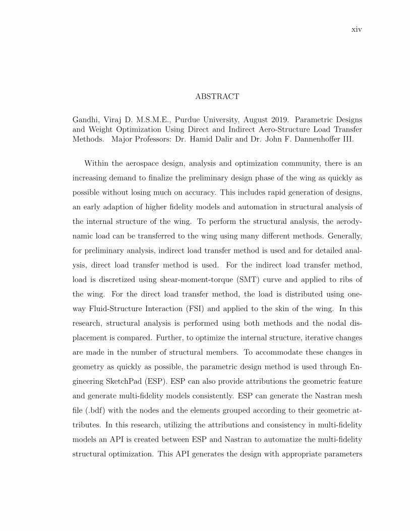
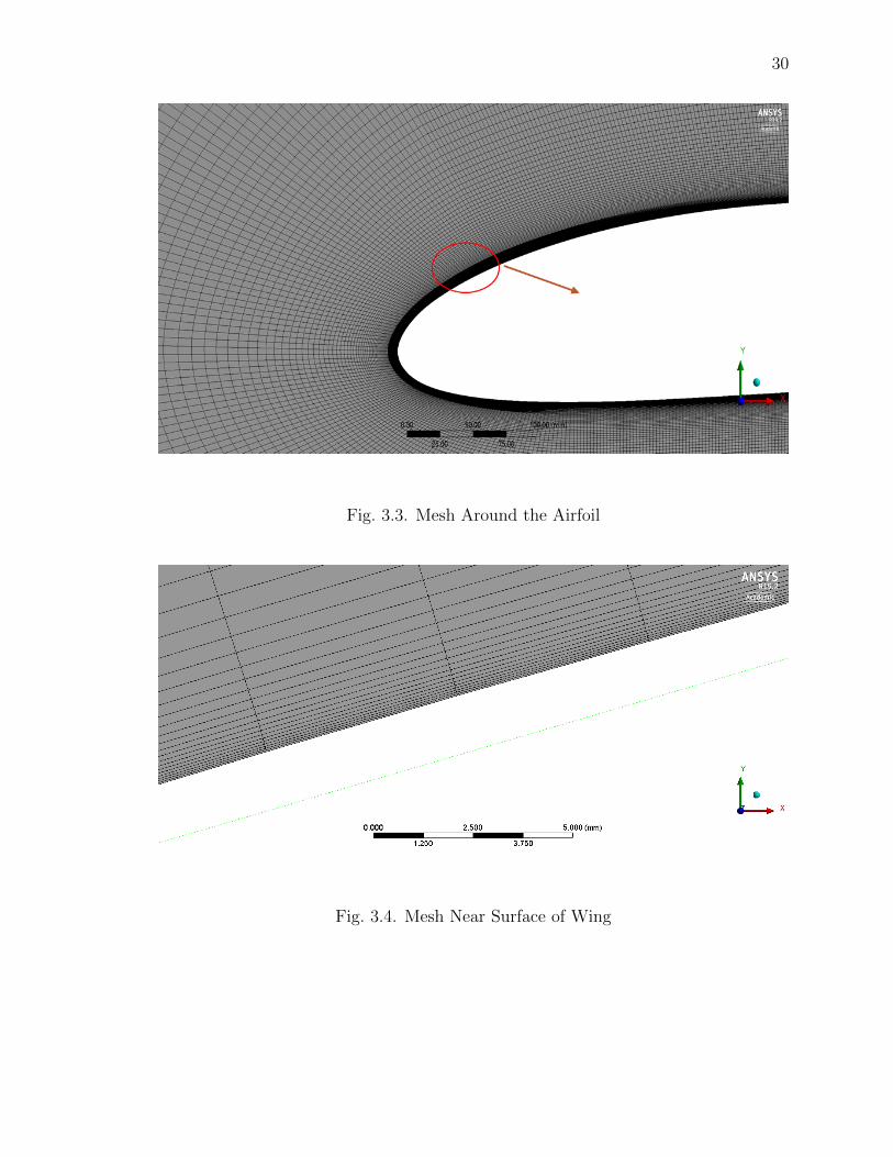
The mesh (Figure 3.3 and Figure 3.4) is generated using boundary layer theories.
As this research is mainly focused on surface pressure and shear forces, it is absolutely
crucial to capture boundary layer. To do that, a certain turbulence model needs
to be used which are fairly stable for maximum y+ value between 1 and 12 [26].
Hexahedron mesh is created using Ansys ICEM module using blocks method. The
Reynolds number is approximately 30 × 106. The boundary layer thickness is 3.5 ×
10−6m. The first cell height is 15 × 10−6m thus the y+ value is 4.3 [6]. The growth
rate is kept at 1.15 and the total elements are 20 × 106.
30
Fig. 3.3. Mesh Around the Airfoil
Fig. 3.4. Mesh Near Surface of Wing

31
3.1.3 Boundary Conditions
To simulate the flow with an angle of attack, the components of velocity is given
in X and Y direction at “inlet”. The root side of the fluid domain is given symmetric
condition. The back side of the domain is given outlet condition. The upper, lower
and tip side of fluid domain are given open condition as shown in Figure 3.5.
Fig. 3.5. Boundary Conditions of Fluid Domain
The open condition is given to simulate semi-infinite side. At the tip, due to
vortex, the flow might enter the domain and this BC allows fluid to come in. While
the pressure outlet condition works as one way valve for each individual element
face [27]. This can be avoided by having a big domain but due to limitations in
computational capabilities, it was not possible. The relative pressure is kept zero at
the outlet and open BC side. The inlet condition is 0.35 Mach number at 7-degree
angle of attack. The surface of the airfoil is a smooth wall with no-slip boundary
condition.

32
3.1.4 Convergence Check and Comparison
As the mesh was generated using boundary layer theories, the convergence of
mesh parameters was obtained fairly quickly. The initial value of first cell height 20
× 10−6 m is chosen. As the area of interest is shear forces at the surface of the wing,
dominating parameters are the height of first cell near the surface and the growth rate.
Table 3.1 and Table 3.2 shows convergence history and Table 3.3 shows calculated
value with XFLR5. XFLR5 predicts the lift and drag coefficient of the wing. The
tool can give only approximate data.
Fig. 3.6. Pressure Contours on The Wing and XY Plane at Z = 5m

33
Table 3.1.Convergence Check (Growth Rate Change)
Boundary layer cell height = 20 ×10−6m
Growth rate Cl
1.250 0.9364
1.200 0.9312
1.150 0.9291
1.100 0.9290
Table 3.2.Convergence Check (Boundary Layer Height Change)
For growth rate = 1.150
Boundary layer cell height (×10−6m ) Cl
20.0 0.9291
15.0 0.9283
10.0 0.9281
8.0 0.9280
Table 3.3.Comparison With XFLR5
Alfa CFD Cl XFLR5 Cl
0 0.3621 0.3744
4 0.6954 0.7152
7 0.9283 0.9426

34
3.2 Structural Analysis
3.2.1 Geometry
The same OML is imported in another DM and the internal structures are created.
The internal structure (i.e. ribs and spars) are generated by intersecting planer sheets
with the solid wing OML so that the sheets get the exact profile of the wing. Then,
the solid OML is converted to sheet OML. All the bodies are condensed to one part
to have shared nodes between different intersecting surfaces. This will ensure the
proper load transfer from the skin of the wing to the structure of the wing. Ribs are
equally spaced while spars are created at 17%, 45% and 73% of chord length shown
in Figure 3.7.
Fig. 3.7. Wing With Internal Structure
35
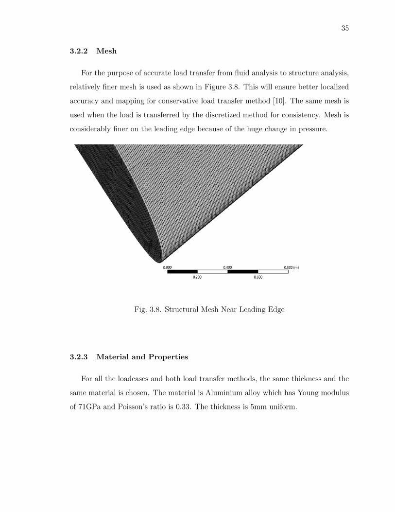
3.2.2 Mesh
For the purpose of accurate load transfer from fluid analysis to structure analysis,
relatively finer mesh is used as shown in Figure 3.8. This will ensure better localized
accuracy and mapping for conservative load transfer method [10]. The same mesh is
used when the load is transferred by the discretized method for consistency. Mesh is
considerably finer on the leading edge because of the huge change in pressure.
Fig. 3.8. Structural Mesh Near Leading Edge
3.2.3 Material and Properties
For all the loadcases and both load transfer methods, the same thickness and the
same material is chosen. The material is Aluminium alloy which has Young modulus
of 71GPa and Poisson’s ratio is 0.33. The thickness is 5mm uniform.

36
3.2.4 Loads on The Wing
Distributed load transfer
For the distributed load transfer method, the pressure from CFD results is di-
rectly transferred to structural grid nodes. For the purpose to transfer pressure and
essentially force, conservative data transfer algorithms need to be used. Here, the
load will be applied to each individual nodes on the skin of the wing. The method is
described in section 3.3.
DIscretized load transfer
In this method, the aerodynamic load is converted into stick model load and then
it is redistributed only on the edge of ribs using RBE3 elements. The master node
is generally created at the geometric center which may or may not be the same as
pressure or force center. The weight function for each slave node is 1. The force and
moments on master nodes are calculated in section 3.4.
Boundary Condition
The root of the wing is constrained in Tx, Ty, and Tz direction. It is complex to
give accurate boundary condition to a wing because, in reality, the root of the wing is
transferring the load to the fuselage and eventually give translation in lift direction.
3.3 Load Transfer Using FSI
After getting the convergence of mesh and a relatively valid agreement with
XFLR5 data, the load can be transferred to structural mesh. In order to do that,
Ansys provides a user interface where the user needs to connect the static structural
model to CFD results. The mesh mapping will be done based on overlapping surfaces
within a marginal distance. The pressure data is then transferred to the required

37
structural nodes from the fluid nodes. There are many algorithms for data transfer
and mapping. Here, as the force needs to be transferred, Conservative Profile Pre-
serving data transfer algorithm needs to be used. The transferred load on the upper
surface is shown below in Figure 3.9.
Fig. 3.9. Load Transfer Using FSI
3.4 Load Transfer Using Stick Model
To transfer the load using stick model approach, the intersection of the wing OML
and fluid domain is divided into subsections as shown in Figure 3.2. The loads on
these sections are calculated independently and concentrated on the geometric center
of each section. This is the location of the node of stick model. A smooth curve of
shear force - bending moment - torque (SMT) joining each node is created. As the

38
number of sections and location of stick model node is independent to the location of
rib, interpolation is done to get the load data at the location of rib. This load is ap-
plied to the master node of RBE3. The whole process is shown below. The coordinate
system is: +X is chordwise direction, +Z is spanwise direction and +Y is lift direction.
Step - 1: Calculate the lift acting on each section by calculating the force on each
element of that section.
Lift =
∮P (x, z) dxdz (3.1)
Step - 2: Calculate the center of pressure for each section which is denoted by Px and
Pz in X and Z direction.
Pressure center [Px, Pz] =
[∫x P (x, z) dxdz∫P (x, z) dxdz
,
∫z P (x, z) dzdx∫P (x, z) dzdx
](3.2)
The representation of the center of pressure is shown in Figure 3.10. The points are
not necessarily on a line.
Step - 3: In this step, the load is transferred from the pressure center to the geometric
center represented in Figure 3.11. This will create moment in the Z direction and X
direction. Also, the bending moment generated due to shear force in each section is
calculated. The geometric center is denoted by Gx and Gz in X and Z direction. The
load calculated in this step is the amount of load which is generated by the section.
Generated loads at the discretized node are:
Force in Y direction (shear force):
Fy = Lift− (fuel + structure weight) ∗G (3.3)
Moment generated in Z direction (torsion):
Mz = − Fy ∗ (Gx− Px) (3.4)

39
Fig. 3.10. Pressure Center of Sections
Bending moment generated in X direction due to shear force (BMSF):
Mx = (−Fy) ∗Gz (3.5)
The moment in X due to the distance between Gz and Pz is usually very small
compared to the moment generated by shear force. Thus, it is usually ignored.
G = gravity force multiplier
In moments, the negative sign comes from the direction of forces.
Step - 4: Find the total load on the wing and generate total load Vs span graph. This
graph shown in Figure 3.12 is also called as SMT graph and the data is given in Table
3.4. Numbering convention on rib starts from the tip. So, the section at the tip is 1st
section. The amount of total load on nth discretized node = load generated on nth
discretized node + total load on (n-1)th discretized node. The example shown here is
for 7 degree angle of attack at Mach number = 0.35. This represents 2.5G loadcase
for bombardier challenger 350 which weighs 18,416 KG [28].

40
Fig. 3.11. Load Transfer from Pressure Center to Geometric Center
Here, the total Mx is around -1275 KN.m that is generated by shear force. Total mo-
ment generated by transferring Fy from Pz to Gz is 4.5 KN.m. So, it can be ignored.
Table 3.4.: Total Load Data
Span (m) Total Fy (N) Total Mz (N.m) Total Mx (N.m)
0.375913 215450.4 -70319.3 -1276262.47
1.12542 208377.5 -69087.3 -1273603.66
1.874597 198589.8 -66794 -1262588.4
continued on next page

41
Table 3.4.: continued
Span (m) Total Fy (N) Total Mz (N.m) Total Mx (N.m)
2.623899 187044 -63804.7 -1240944.69
3.373339 174103.6 -60129.7 -1206990.41
4.122748 159953.8 -55767.4 -1159258.37
4.872148 144726.7 -50723.2 -1096480.89
5.62156 128541.1 -45016.6 -1017622.42
6.370835 111518.2 -38686.7 -921926.834
7.119978 93783.02 -31797.6 -808939.167
7.868783 75472.9 -24449.6 -678571.469
8.616797 56742.79 -16797.3 -531188.324
9.361831 37774.46 -9102.14 -367742.07
10.11266 18784.47 -1869.56 -189960.999
Step - 5: The aerodynamics department gives the graph generated above to the struc-
tural analysis department. To perform structural analysis, interpolation needs to be
done at the rib location to get the total load. Here, the numbering starts from the
tip. The tip rib being external is given number ‘0’. One thing to notice in the graph
is it doesn’t end at tip location nor it starts from the root. The amount of total load
on 0th rib is given below.
Total load on 0th rib = load on 1st discretized node ∗ a
width of section(3.6)
a = min (distance between 1st rib to 1st discretized node, width of section)
If the width of the section is not known by the structural analysis team, the load on
0th rib is half of the load on 1st discretized node.

42
Fig. 3.12. Shear-Moment-Torque
Step - 6: Now, the total load needs to be converted to the applicable load on each
rib. For the 0th rib, the applicable load is equal to the total load. For nth rib, the
equations are listed below.
For shear force (Fy):
applicable Fy on nth rib = total Fy on nth rib− total Fy on (n− 1)th rib (3.7)

43
For torsion (Mz):
applicable Mz on nth rib = total Mz on nth rib− total Mz on (n− 1)th rib (3.8)
For bending moment (Mx):
applied Mx on nth rib = total Mx on nth rib−BMSF (3.9)
These loads are applied to master node on RBE3 elements of ribs. The RBE3 elements
are represented in Figure 3.13. The discretized load on wing is represented in Figure
3.14. Here, the skin is hidden.
Fig. 3.13. RBE3 on Edge of Rib
3.5 Result and Comparison
For comparison, 3 loadcases are analyzed. One is critical loadcase that is at 7
degree angle of attack which replicates 2.5 G at taking off; another is 4 degree angle
of attack which replicates 1.6 G; the last is 0 degree angle of attack which replicates 1
G cruising. In all the cases, the Mach number is kept fixed at 0.35. The deformation
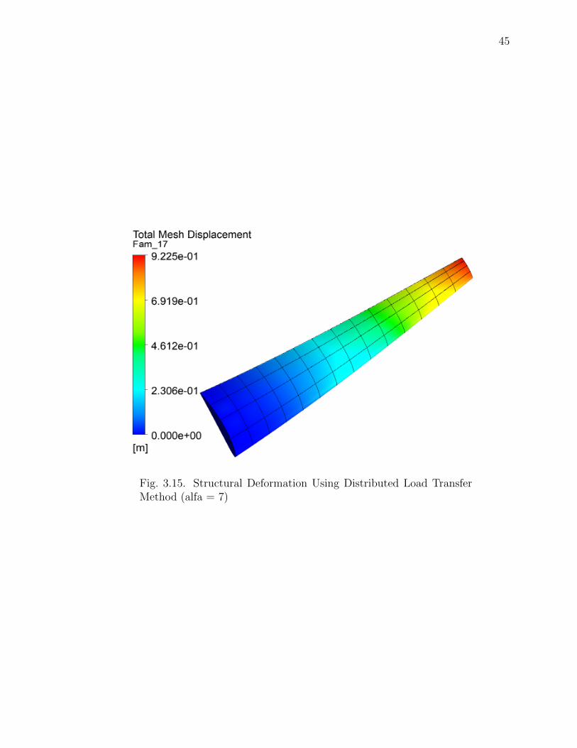
from the leading edge and the trailing edge is taken as output and compared. Figure
3.15 and Figure 3.16 shows the deformation is similar and the graph in Figure 3.17
and Figure 3.18 agrees with that.
As it can be seen from Figure 3.17 and Figure 3.18 that both lines coincide on
each other throughout the span. The difference at maximum deformation is 0.27%.
Similar behavior can be seen for the other two cases as well shown in Figure 3.19 and
Figure 3.20.

44
Fig. 3.14. Load Applied Using Discretized Load Transfer Method
Table 3.5.Difference in Maximum Deformation
Alfa Max difference (mm) % difference at max deformation
0° 5.59 1.46
4° 2.41 0.34
7° 2.49 0.27
3.6 Conclusion
Discretized load transfer method provides results as accurately as distributed load
transfer method up to at least 9.09 aspect ratio for preliminary design phase.
45
Fig. 3.15. Structural Deformation Using Distributed Load TransferMethod (alfa = 7)

46
Fig. 3.16. Structural Deformation Using Discretized Load TransferMethod (alfa = 7)

47
Fig. 3.17. Deformation vs Span at Leading Edge (Alfa = 7)

48
Fig. 3.18. Deformation vs Span at Trailing Edge (Alfa = 7)
(a) Deformation vs Span at leading edge (b) Deformation vs Span at trailing edge
Fig. 3.19. Deformation vs Span (Alfa = 4)

49
(a) Deformation vs Span at leading edge (b) Deformation vs Span at trailing edge
Fig. 3.20. Deformation vs Span (Alfa = 0)
50
4. WEIGHT OPTIMIZATION OF WING USING
INDIRECT LOAD TRANSFER METHOD
This chapter focuses on the automatization of multi-fidelity optimization of the struc-
tural aspects of the wing. ESP is used to create parametric attributed geometry which
maintains consistency between structural models with different fidelity levels. A stiff-
ness based strategy is used to map the nodal data of the lower-order fidelity structural
models onto the higher-order ones to perform buckling analysis. To demonstrate the
approach, a wing is being optimized to withstand with two separate loadcases. An
API is created to connect the ESP, Nastran, load file and design configuration file in
CSV format.
4.1 User Inputs
To optimize the internal structure, the API takes the geometric and optimization
parameters from user in the form of CSV files. The ribs are equally spaced throughout
the span. The spars are equally spaced between the first and last spar. In the file
user needs to provide the following information:
1. Geometry parameters
(a) Area
(b) Sweep angle
(c) Taper ratio
(d) Aspect ratio
(e) Fractional distance in the chordwise length for the first spar
(f) Fractional distance in the chordwise length for the last spar

51
2. Load parameters
(a) Number of loadcase
(b) Factor of Safety (FS) for static structural optimization
(c) FS for buckling optimization
3. Number of support member (min and max)
(a) Ribs
(b) Spars
(c) Stiffeners
4. Thicknesses (min and max)
(a) Panel
(b) Stiffener
(c) Rib
(d) Spar
In another CSV file, loadcase as shown in Figure 4.1 needs to be provided. Here,
+Y is lift direction, +Z is spanwise direction and +X is chordwise direction. The
structure can be optimized for any number of loadcases. These loads are total loads
on the system at the location. These load cannot be directly applied on the ribs. The
conversion of the total load to the applicable load is described in section 3.4 step-6.
4.2 Geometry Script
Here, a detailed method of wing creation and attribution is displayed which is
used in further analysis. First, two NACA profiles are created based on parameters
provided by the user as it can be seen in Table 4.1. Then they are ruled to create
Outer Mold Layer (OML) of wing. The upper surface is attributed as “upper skin”

52
Fig. 4.1. Loadcase CSV File
and lower surface as “lower skin”. The leading edge and trailing edge are attributed
as “leading edge” and “trailing edge”. The waffle is created based on parameters
of internal structure. The waffle is intersected with solid wing so that the internal
structure will have the exact profile of the wing. The waffle is then subtracted from
solid wing to create the scribed wing. This scribed wing is then converted to sheet
body using “extract” command. The internal structure and sheet wing are unioned to
create one continuous structure. While making waffle, each ribs and spars are given
attributes. Ribs are identified as name = “Rib” and index = 1,2,3,. . . as shown in
Figure 4.2. The airfoil at the tip is also attributed as Rib with index = nRib+1. The
root airfoil is given attribute “Root”. The spars are identified as name = “Spar” and
index = 1,2,3,. . . The panels are identified by the index of rib on the tip side and spar
index on the trailing side. For example, as given in Figure 4.3, the panel attribute is
U3 2. Here, U is for upper surface; index of the rib on the tip side of panel is 3 and
index of the spar on trailing side is 2. All the edges of the panels are also given the
attributes of the panel as shown in Figure 4.6. Based on attributes on face of ribs,

53
spars and panel of the wing, the required edge attributed as “RBE3 1,2,3,. . . ”. The
panels attached to trailing edge is given an attribute as “ignoreNode=true” which
allows the element associated with the surfaces to not to be present in the Nastran
bulk (.bdf) file. This bdf file is used to perform static structural analysis on the wing.
Each panel is dumped with extension of .EGADS; later to be imported again into
ESP for buckling analysis. The whole flowchart is given in Figure 4.4.
Table 4.1.Design Parameters of Wing and Panels
Parameter name Value Description
series w 4409 NACA profile of the wing
area 10 m2 area of the wing
aspect 6 aspect ratio of the wing
taper 0.7 taper ratio of the wing
sweep 20 sweep angle of the wing
nrib 5 number of ribs in the wing
xfirst 0.2 fraction distance in the chordwise length for
the first spar
xlast 0.75 fraction distance in the chordwise length for
the last spar
nspar 3 number of spars in the wing
nstiff 3 number of stiffeners on the wing panel
depth -0.01 depth of the stiffener
angle 45 angle of the runoffs at the ends of the stiffener
Further, to optimize the wing for buckling mode, each panel needs to be stiffened.
As the stiffeners are discontinuous, they don’t play an important role in material
failure but they are very important for buckling stability. For that, the dumped
panels are imported and are stiffened using a User Defined Function (UDF) called

54
“stiffeners”. UDF stiffeners create surfaces perpendicular to the local surface on the
panel for a given depth. It also generates runoffs at the end of stiffeners. These
parameters are also given in Table 4.1
Fig. 4.2. Rib Attributions
4.3 Analysis Setup
To perform optimization automatically, the API works as pre-processor to apply
material property, boundary conditions, data transfer between different fidelity, etc.
It reads the load data, geometric and optimization parameters from separate CSV
files. The API also works as postprocessor and makes the decision about change in
the number of structural members. It generates CSM for ESP and gets the attributed
mesh from ESP.

55
Fig. 4.3. Example of Panel Attribution
4.3.1 Static Structural Failure Mode
After completing the geometry generation and attribution on surfaces, ESP dumps
the mesh file in a .bdf format which has attribution on nodes and elements. For the
material failure of the wing, in Global Finite Element Model (GFEM), stiffeners are
not modeled. As the stiffeners are not continuous, they do not provide rigidity against
static failure. In this mesh file, nodes and the elements grouped according to their
geometric attributes. Using these attributes, the elements of each panel is identified
and given separate property ID (PID). All the ribs are given the same PID and all
spars have the same PID. To transfer the load on the wing, RBE3 master nodes are
generated at the geometric center of each rib. The edge nodes shown in Figure 4.5 are
connected to the master node. These nodes are also identified based on attribution
(i.e. RBE3 1, RBE3 2. . . ). Here, a conservative approach is taken in which all the
loads are assumed to be taken by wingbox.

56
Fig. 4.4. Flowchart for Geometry Script
After differentiating between element properties and generation of new elements,
loads can be applied on RBE3 master nodes. The master node distributes the load
on slave nodes based on screw theory. These loads are provided by the user in CSV
file as shown in Figure 4.1. If the location of stick model nodes and location of

57
Fig. 4.5. RBE3 Connection
RBE3 master nodes doesn’t match, interpolation is done. The root is given fixed
constraints. The new bdf file is generated which includes Nastran executive controls,
case-control, bulk data, and optimization control data. The optimization control
data contains variables (i.e. the thickness of each PID), constraints (i.e. max stress)
and an objective function (i.e. minimize weight). The bdf file is sent to Nastran to
optimize using SOL 200 for static structural failure mode. The optimization is done
on all provided loadcases. The minimum thickness for each PID for nth loadcase is
equal to optimized thickness for (n-1)th loadcase. Minimum thickness for 1st loadcase
is provided by the user.
4.3.2 Buckling Failure Mode
Further, for buckling stability, the deformation data of each loadcase needs to
be transferred from lower fidelity to higher fidelity model for overall optimization.
To do that, static structural analysis needs to be performed to get deformation on
58
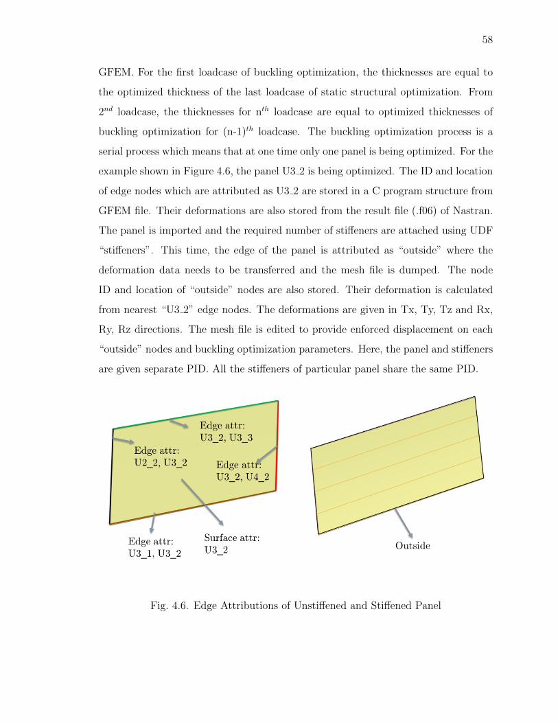
GFEM. For the first loadcase of buckling optimization, the thicknesses are equal to
the optimized thickness of the last loadcase of static structural optimization. From
2nd loadcase, the thicknesses for nth loadcase are equal to optimized thicknesses of
buckling optimization for (n-1)th loadcase. The buckling optimization process is a
serial process which means that at one time only one panel is being optimized. For the
example shown in Figure 4.6, the panel U3 2 is being optimized. The ID and location
of edge nodes which are attributed as U3 2 are stored in a C program structure from
GFEM file. Their deformations are also stored from the result file (.f06) of Nastran.
The panel is imported and the required number of stiffeners are attached using UDF
“stiffeners”. This time, the edge of the panel is attributed as “outside” where the
deformation data needs to be transferred and the mesh file is dumped. The node
ID and location of “outside” nodes are also stored. Their deformation is calculated
from nearest “U3 2” edge nodes. The deformations are given in Tx, Ty, Tz and Rx,
Ry, Rz directions. The mesh file is edited to provide enforced displacement on each
“outside” nodes and buckling optimization parameters. Here, the panel and stiffeners
are given separate PID. All the stiffeners of particular panel share the same PID.
Fig. 4.6. Edge Attributions of Unstiffened and Stiffened Panel

59
The buckling optimization for each panel is repeated until the maximum number
of stiffeners are attached. From this, the combination of thicknesses and number of
stiffener which gives minimum weight is selected as the optimized combination for a
particular panel. For buckling optimization, the value of the minimum thickness for
skin and stiffeners and the minimum number of stiffeners for nth loadcase is equal to
optimized parameters for (n-1)th loadcase. The minimum thicknesses of panels for
1st loadcase is equal to optimized thickness for the last loadcase of static structural
analysis. Minimum thickness and number of stiffener is defined by user. The process
is repeated for all the panels except for ailerons as it is assumed that they don’t take
any load. The process of buckling optimization is repeated for all the loadcases. The
whole process from static structural optimization is repeated for all possible combi-
nation of ribs and spars. The combination of thicknesses and number of structural
members which satisfy both failure modes and generates minimum weight is selected
as optimized design. The flowchart for the analysis process is shown in Figure 4.7.
4.4 Results
The wing with given geometry parameters in Table 4.1 and for loadcases shown
in Figure 4.1 is optimized. The constrain is 500MPa with FS for static structural and
buckling is 1.2 and 1.1 respectively. The range of thicknesses for all surfaces is 8mm
to 1mm. Number of ribs varies from 3 to 6 and number of spars are fixed 3. Number
of stiffeners varies from 0 to 4. The results of overall optimized geometry have 5 ribs
and 3 spars. The rib thickness is 1.19mm and spar thickness is 4.47mm. the overall
weight of the wing is 84.6 KG. The details about the panels are shown in Table 4.2.
The results are shown in Figure 4.8 and Figure 4.9.

60
Table 4.2.: Results of Optimized Geometry
Panel name Number of Thickness of Thickness of Weight
stiffeners panel (mm) stiffeners (mm) (KG)
U1 1 3 2.02 1.07 1.45
U2 1 3 2.53 1.63 1.74
U3 1 3 2.79 1.73 1.78
U4 1 3 2.47 1.64 1.49
U5 1 3 2.10 1.52 1.18
U6 1 3 1.42 1.00 0.72
U1 2 2 4.98 1.00 3.64
U2 2 3 4.33 2.59 3.38
U3 2 3 4.46 2.62 3.32
U4 2 3 4.00 2.51 2.86
U5 2 3 3.71 2.47 2.56
U6 2 3 2.80 1.68 1.80
U1 3 3 3.86 1.56 3.02
U2 3 3 3.13 2.72 2.61
U3 3 3 3.42 3.88 2.89
U4 3 3 3.67 2.92 2.75
U5 3 3 3.28 2.16 2.26
U6 3 3 1.98 1.00 1.23
L1 1 3 2.13 1.00 1.41
L2 1 2 1.97 1.08 1.18
L3 1 3 1.78 1.43 1.13
L4 1 2 1.95 1.42 1.03
L5 1 2 1.69 1.22 0.82
L6 1 0 1.00 1.00 0.34
continued on next page

61
Table 4.2.: continued
Panel name Number of Thickness of Thickness of Weight
stiffeners panel (mm) stiffeners (mm) (KG)
L1 2 2 4.67 1.65 3.50
L2 2 3 3.24 1.00 2.36
L3 2 2 2.87 1.26 1.98
L4 2 3 2.50 1.00 1.69
L5 2 3 1.95 1.00 1.29
L6 2 3 1.55 1.00 1.01
L1 3 2 4.82 1.00 3.52
L2 3 3 2.60 1.39 1.99
L3 3 3 2.14 1.11 1.56
L4 3 3 2.21 1.00 1.51
L5 3 3 1.78 1.00 1.19
L6 3 0 1.00 1.00 0.53
4.5 Conclusion
It is possible to optimize the wing for both the failure criteria without any human
input by careful use of attributes. This approach can be applied to the whole aircraft
if needed. However, the author suggests to make two layers of API. One API for
general purpose analysis in which the user can apply any load on any attributes
which can be given using GUI. Another program can be built on top of first API to
run the analysis or optimization in a loop.

62
Fig. 4.7. Flowchart for Analysis Process

63
Fig. 4.8. Optimized Upper Surface
Fig. 4.9. Optimized Lower Surface

64
5. PARAMETRIC DESIGN OF AIRCRAFT USING
ENGINEERING SKETCHPAD (ESP)
In this chapter, a comprehensive method to create a parametric model of aircraft is
shown. For commercial aircraft and for fighter aircraft, some techniques are different
but the general idea of Outer Mold Layer (OML) and internal structure remains the
same. The final goal is to extend the idea of single button optimization of the wing
to single button optimization of aircraft and this is the first step in the direction.
5.1 Military Aircraft Prototype Syntheses
The master models in ESP are defined in terms of a feature tree and a set of
design parameters. This tree depicts the sequence of the operations used to create
the final design which can be extracted from the CSM file and is shown in Figure 5.1.
Fig. 5.1. ESP Tree Structure to Generate a Military Fighter Aircraft

65
In this tree structure, each part contains several steps. These steps are called
‘Branches’. Each part starts with the generation of standard primitives which includes
Box, sphere, cone, cylinder, or torus. Some branches are used to grow sketches such
as extrude, rule, blend, revolve, sweep, or loft. And some are User Defined Primitives
(UDP) such as ‘Naca’ and ‘supell’ (superellipse). ESP arranges bodies in a stack
order approach. This means that a given command is being operated on the last
generated body or the last two bodies in case of the Boolean operations.
The section “nose to nozzle using blend” is divided into three sections. First, the
super-elliptical sheets are created to generate cone section of the body. It all sheets
were blended with a nose radius. Second, the cylindrical section is created which
is between nose and nozzle. Third, the nozzle section is created and unioned them
together shown in Figure 5.2. The wing and the stabilizers are created by creating
naca profile at the required location and ruling them together. Then all the parts are
unioned to form complete OML represented in Figure 5.3.
Fig. 5.2. Middle Section of Aircraft

66
Fig. 5.3. Solid OML
For unibody design of the internal structures, two separate waffles need to be
created. One for vertical stabilizers (Figure 5.4) and another for remaining of the
structure (Figure 5.5). Both waffle shares line contact with each other and they are
connected using the “join” command to generate structure shown in Figure 5.6. This
is the key step in the generation of continuous internal structure. The waffle is then
subtracted from the OML, which enforces the outer sheet Body to be scribed by the
faces of the waffle. The waffle is then intersected with solid OML (non-scribed) to
create internal structure with the exact shape of OML (Figure 5.7). The scribed OML
is converted to sheet OML and unioned with internal structure. From this unibody,
the cockpit section and the engine section are subtracted.
Table 5.1 shows the design parameters used in building the parametric model
of the aircraft. The three models shown in Figure 5.8 are different in terms of the
configuration of their aerodynamic parameters and internal structures. The design
parameters of each model have been depicted in Table 5.2.

67
Fig. 5.4. Waffle for Vertical Stabilizer
Table 5.1.: Design Parameters
Parameter name Value Description
cone radius 0.25 Radius of nose cone
cone length 1.2 Length of nose cone
cockpit length 5.5 Length of cockpit
cockpit num 3 Frame number in cockpit
cockpit width 2.0 Width of cockpit
engine length 4.5 Length of engine
engine num 2 Width of engine
engine width 4.0 Frame number in engine
spars num 6 Number of spars
spars initial length 20.0 Length of wing at root
continued on next page
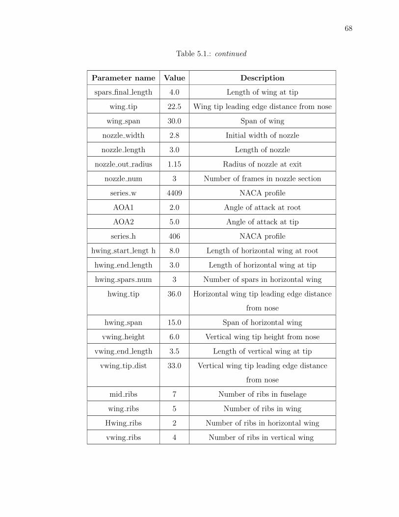
68
Table 5.1.: continued
Parameter name Value Description
spars final length 4.0 Length of wing at tip
wing tip 22.5 Wing tip leading edge distance from nose
wing span 30.0 Span of wing
nozzle width 2.8 Initial width of nozzle
nozzle length 3.0 Length of nozzle
nozzle out radius 1.15 Radius of nozzle at exit
nozzle num 3 Number of frames in nozzle section
series w 4409 NACA profile
AOA1 2.0 Angle of attack at root
AOA2 5.0 Angle of attack at tip
series h 406 NACA profile
hwing start lengt h 8.0 Length of horizontal wing at root
hwing end length 3.0 Length of horizontal wing at tip
hwing spars num 3 Number of spars in horizontal wing
hwing tip 36.0 Horizontal wing tip leading edge distance
from nose
hwing span 15.0 Span of horizontal wing
vwing height 6.0 Vertical wing tip height from nose
vwing end length 3.5 Length of vertical wing at tip
vwing tip dist 33.0 Vertical wing tip leading edge distance
from nose
mid ribs 7 Number of ribs in fuselage
wing ribs 5 Number of ribs in wing
Hwing ribs 2 Number of ribs in horizontal wing
vwing ribs 4 Number of ribs in vertical wing

69
Fig. 5.5. Waffle Without Vertical Stabilizer
Table 5.2.Design Parameters for Figure 5.8
Number of Ribs Number of Spars Wing tip distance
Figure 5.8.a 3 3 25
Figure 5.8.b 4 4 25
Figure 5.8.c 3 3 22.5

70
Fig. 5.6. Continuous Waffle
Fig. 5.7. Internal Structure

71
Fig. 5.8. Aircraft with Different Configurations

72
6. CONCLUSIONS AND FUTURE WORK
6.1 Conclusion
• For low to medium aspect ratio of wing for the preliminary design phase, the
discretized load transfer method provides almost the same results as the dis-
tributed load transfer method. However, discretization of the load is a relatively
tedious process but necessary for the visualization of load characteristics.
• If the design of OML and internal structure; both are being changed iteratively,
transferring load using the distributed load transfer method can be preferable.
• Using the attributes of the geometric features as KeyWords, connection between
ESP and analysis software is possible by creating appropriate API.
• Automatization of preprocessing and multi-fidelity load transfer can simplify
the erring process and can save time.
• Parametric design method is very useful when creating a family of products
which shares the same geometric features. However, this approach might be
overkill if a quick investigation of 3D design needs to be done at a conceptual
phase.
6.2 Future Scope
• Extension of the single button optimization on the whole aircraft
• Methods to transfer load from wing to fuselage needs to be developed and
applied to analyze the whole jet simultaneously.
• The optimization of panels can be done in parallel.

73
• Instead of tailoring API for specific analysis, a general purpose API to connect
ESP and Nastran can be created. This API can apply loads, BC and properties
based on attributes.
• This API can be created to connect with different solver and not only structural
solver but fluid solvers also.
• The general purpose API can be used to couple fluid analysis and structural
analysis to perform one-way or two-way FSI for the detailed design phase.

REFERENCES

74
REFERENCES
[1] B. Rose, G. Jinu, and M. Manivel, “Partly coupled fluid structure interactionanalysis of an aircraft wing at subsonic speeds,” International Journal of Me-chanical & Mechatronics Engineering, vol. 14, no. 3, pp. 22–29, 2014.
[2] V. Gandhi, J. Joe, J. Dannenhoffer, and H. Dalir, “Multifidelity structural designand analysis of aircraft structures using engineering sketch pad and nastran,” inAIAA Scitech 2020 Forum, January 2020.
[3] R. Haimes and J. Dannenhoffer, “The engineering sketch pad: A solid-modeling,feature-based, web-enabled system for building parametric geometry,” in 21stAIAA Computational Fluid Dynamics Conference, 2013, p. 3073.
[4] Nasa Glenn Research Center, Boundary Layer, (accessed July 20, 2019). [Online].Available: https://www.grc.nasa.gov/WWW/k-12/airplane/boundlay.html
[5] F. M. White, Viscous fluid flow, 3rd ed. McGraw-Hill New York, 2006, pp.75–78.
[6] Pointwise, Y+ Calculator, (accessed July 20, 2019). [Online]. Available:http://www.pointwise.com/yplus/
[7] Autodesk, SST K-w Turbulence Model, (accessed July 20, 2019). [Online].Available: https://knowledge.autodesk.com/support/cfd/learn-explore/caas/CloudHelp/cloudhelp/2014/ENU/SimCFD/files/GUID-0F5C4828-9F91-46B6-A16A-2578D72DCFCC-htm.html
[8] Ansys, FLUENT 6.3 User’s Guide - 12.5.2 Shear-Stress Transport (SST) -Model, (accessed July 20, 2019). [Online]. Available: https://www.sharcnet.ca/Software/Fluent6/html/ug/node487.htm
[9] H.-J. Bungartz and M. Schfer, Fluid-Structure Interaction: Modelling, Simula-tion, Optimisation. Springer, 01 2006.
[10] Ansys, Ansys Coupling User Guide. Ansys User Guide, 2016, pp. 65–72.
[11] P. Galpin, R. Broberg, and B. Hutchinson, “Three-dimensional navier stokespredictions of steady state rotor/stator interaction with pitch change,” in Pro-ceedings of 3rd Annual Conference of the CFD Society of Canada, Banff, AB,Canada, vol. 3, 1995.
[12] Mike and A. Canard, XFLR5, (accessed July 20, 2019). [Online]. Available:http://www.apollocanard.com/6 xflr5.htm
[13] S. Batchu, RBE2 Vs RBE3, (accessed July 20, 2019). [Online]. Available:http://www.stressebook.com/rbe2-vs-rbe3/

75
[14] Quartus Engineering, NASTRAN 101, (accessed July 20, 2019). [Online].Available: https://www.quartus.com/resources/nastran-101
[15] MSC.software, Nastran Quick Reference Guide. MSC.software, 2017.
[16] MSC.software, Design Optimization, (accessed July 20, 2019). [Online].Available: https://www.mscsoftware.com/application/design-optimization
[17] M. Brunelli, Parametric vs. Direct Modeling, (accessed July 20, 2019). [Online].Available: https://www.ptc.com/en/cad-software-blog/parametric-vs-direct-modeling-which-side-are-you-on
[18] DesignTech, Parametric Modelling, Process, Advantages and ParametricModelling Tools, (accessed July 20, 2019). [Online]. Available: https://www.designtechsys.com/articles/parametric-modelling
[19] J. Dannenhoffer, “Opencsm: An open-source constructive solid modeler formdao,” 51st AIAA Aerospace Sciences Meeting including the New Horizons Fo-rum and Aerospace Exposition, no. 0701, 2013.
[20] R. Haimes and M. Drela, “On the construction of aircraft conceptual geometryfor high-fidelity analysis and design,” in 50th AIAA Aerospace sciences meetingincluding the new horizons forum and aerospace exposition, 2012, p. 683.
[21] OPEN CASCADE, OpenCascade, (accessed July 20, 2019). [Online]. Available:http://www.opencascade.org
[22] Wikiwand, Wikiwand, (accessed July 20, 2019). [Online]. Available: https://www.wikiwand.com/en/Chord (aeronautics)
[23] C. L. Ladson, C. W. Brooks, and A. S. Hill, “Computer program to obtainordinates for naca airfoils,” NASA Technical Memorandum, Report, 1996.[Online]. Available: https://ntrs.nasa.gov/archive/nasa/casi.ntrs.nasa.gov/19970008124.pdf
[24] AirfoilTools, NACA 4 digit airfoil generator, (accessed July 20, 2019). [Online].Available: http://airfoiltools.com/airfoil/naca4digit
[25] S. Hiremath and A. Malipatil, “Cfd simulation of aircraft body with differentangle of attack and velocity,” International Journal of Innovative Research inScience, Engineering and Technology, vol. 3, 2014.
[26] D. Creech, Can someone explain the Y plus value, (accessed July 20,2019). [Online]. Available: https://www.cfd-online.com/Forums/main/861-can-someone-explain-y-plus-value.html
[27] SAS IP, 2.3.3.Using Inlets, Outlets and Openings, (accessed July 20,2019). [Online]. Available: https://www.sharcnet.ca/Software/Ansys/16.2.3/en-us/help/cfx mod/i5500692.html
[28] M. Thurber, Bombardier Challenger 300 - Wikipedia, (accessed July 20, 2019).[Online]. Available: https://en.wikipedia.org/wiki/Bombardier Challenger 300