parameterizing the effects of leads upon the atmosphere ... · parameterizing the effects of leads...

Parameterizing the effects of leads upon the atmosphere and surface fluxes of the

Arctic Ocean

Photo by Lars Kaleschke, published on phys.org

Steven K. Krueger1, James R. Stoll1, Courteny Strong1, and Hongjie Xie2

1University of Utah, Salt Lake City, USA 2University of Texas, San Antonio, USA

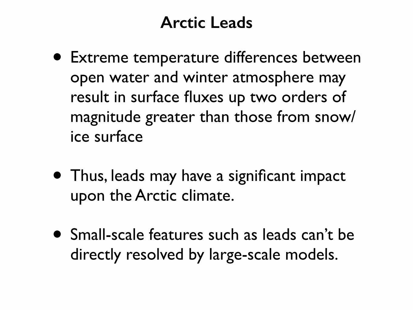
• Extreme temperature differences between open water and winter atmosphere may result in surface fluxes up two orders of magnitude greater than those from snow/ice surface

• Thus, leads may have a significant impact upon the Arctic climate.

• Small-scale features such as leads can’t be directly resolved by large-scale models.

Arctic Leads

Remote Sensing of Leads at SHEBA

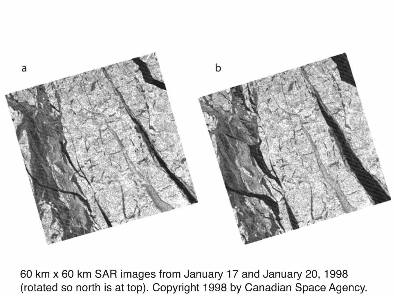
60 km x 60 km SAR images from January 17 and Jan-uary 20, 1998 (rotated so north is at top). Copyrightc⃝1998 by Canadian Space Agency.

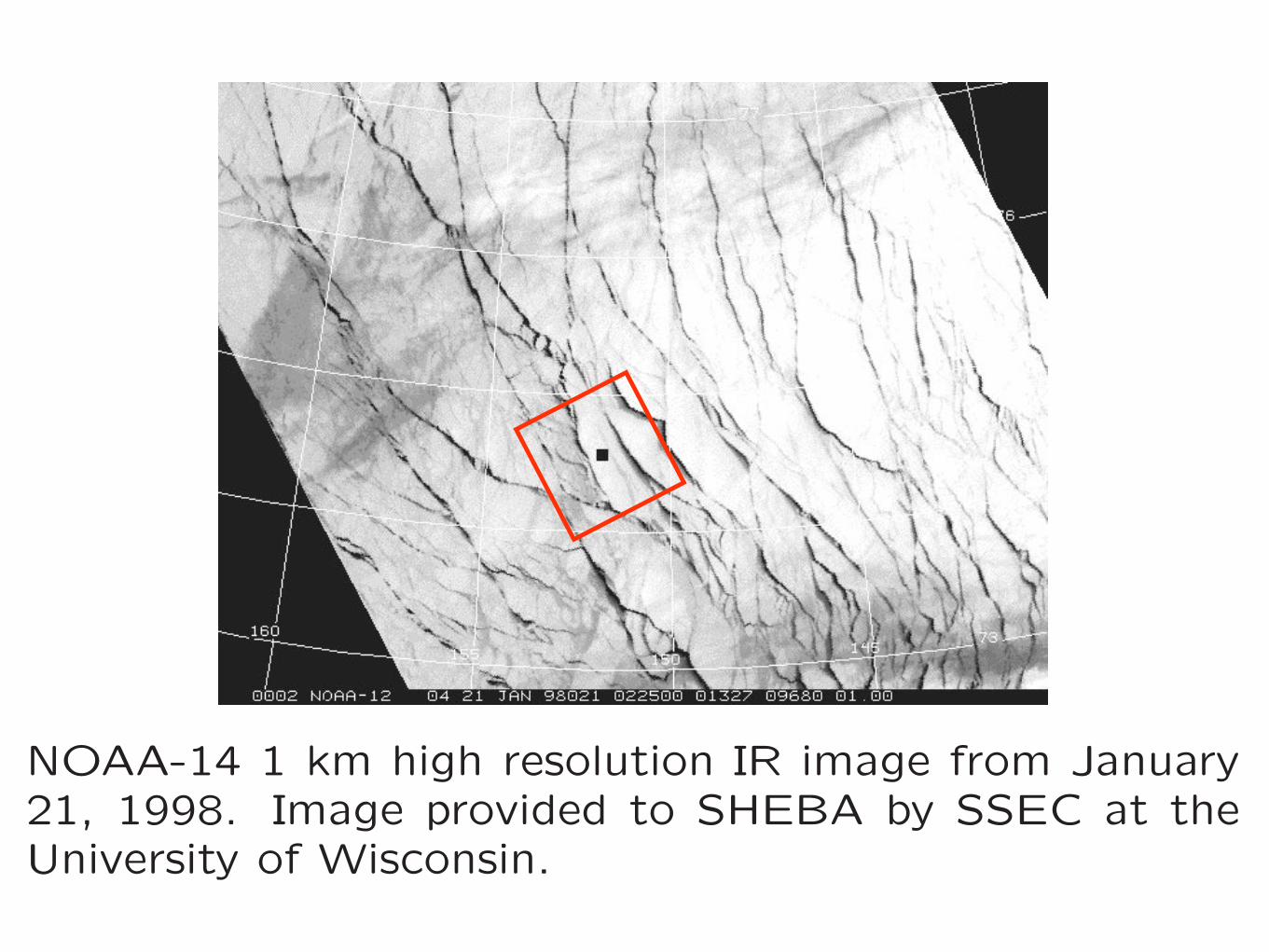
NOAA-14 1 km high resolution IR image from January21, 1998. Image provided to SHEBA by SSEC at theUniversity of Wisconsin.

22

used, 4.5 ! 10"4 m [Persson et al., 1997]. For reasons ofexpediency, we used a constant value of 1.0 ! 10"4 m overthe water surface of an open lead, rather than a fetch or sea-state-dependent value such as used by Alam and Curry[1998]. Finally, the surface temperature of the water isdefined as a constant, "2!C, because the CRM does notpresently simulate the lead freezing process.

4.2. Observations of Leads During SHEBA

[26] Owing to the perpetual darkness of the polar winter,very few direct observations of wintertime leads are avail-able from SHEBA. The existence of leads, as well as theirsize and location, were verified, however, through the use ofvarious types of remote sensing. Very detailed images wereobtained through the use of synthetic aperture radar (SAR)(RADARSAT Images of SHEBA, distributed by H. Stern,http://psc.apl.washington.edu/Harry/Radarsat/, Copyright# 1998 by Canadian Space Agency, SAR imagery pro-cessed at the Alaska SAR Facility (Fairbanks) and distrib-uted through the SHEBA Project Office (Seattle)). Figure 4displays SAR imagery from the Canadian RADARSATsatellite for 17 January and 20 January 1998.[27] These images clearly display the opening of a large

lead approximately 15 km to the east (and approximatelyupwind based on the large-scale wind field) of the SHEBAice camp. In the second image, the lead has attained a widthof up to 8 km, though the portion directly upwind of the icecamp is closer to 3–4 km wide. In addition, other leadshave opened in the vicinity as well. Furthermore, therawinsonde data (as well as the PAM station data, etc.)show that the predominant large-scale surface wind is froma northeasterly direction, so that the near-surface air crossedthe large lead (and others nearby) nearly perpendicularlyprior to reaching the SHEBA site. Satellite IR imagery may

also be used to provide useful information of lead coverageover wide areas.[28] For atmospheric and surface conditions such as these,

it would not be surprising to see some signature of the largeleads and associated convective plumes in the observations atthe ice camp. Lidar imagery (J. Intrieri, SHEBA: LIDAR,ETL DABUL System; Quick-look PRELIMINARY datafrom Ice Camp, http://www.joss.ucar.edu/cgi-bin/codiac/dss?13.302, 1999) from 20 January (Figure 5), displays apossible consequence of the large new openings in the ice. Alow-level cloud layer was observed from approximately 0400UTC to 2000 UTC. The cloud base was typically 100 to 200m above the surface, with a thickness of up to approximately200 m. Unfortunately, owing to the localized nature of theobservations taken at the SHEBA site, it is impossible toknow for certain if these clouds are indeed related to the leadactivity.

5. Resolved Lead Simulation

[29] On the basis of the conditions described in section 4, aseries of simulations was executed. The basic simulationfeatured a 3.2-km-wide lead in a 51.2 km domain. The leadfraction of 6.25% is larger than the average value of 1–2%,but may be more representative of the conditions during ice-divergence events such as that observed near the SHEBA icecamp around 20 January 1998. The orientation of the simu-lated lead relative to the large-scale wind field corresponds tothat of the large lead that occurred upwind of the SHEBA site.[30] Figure 6 displays vertical cross sections from the

basic simulation described above; the fields are displayed at1.5 hours and include the change from the initial conditionsin water vapor mixing ratio, the total cloud ice mixing ratio,the change in potential temperature, and the net upward IR

Figure 4. The 60 km ! 60 km SAR images from (a) 17 January and (b) 20 January 1998 (rotated sonorth is at top). The ship is at center. Note the large wedge-shaped lead several kilometers to the east.Copyright # 1998 by Canadian Space Agency.

ACL 7 - 6 ZULAUF AND KRUEGER: MODELING THE EFFECTS OF ARCTIC LEADS

60 km x 60 km SAR images from January 17 and January 20, 1998 (rotated so north is at top). Copyright 1998 by Canadian Space Agency.

33

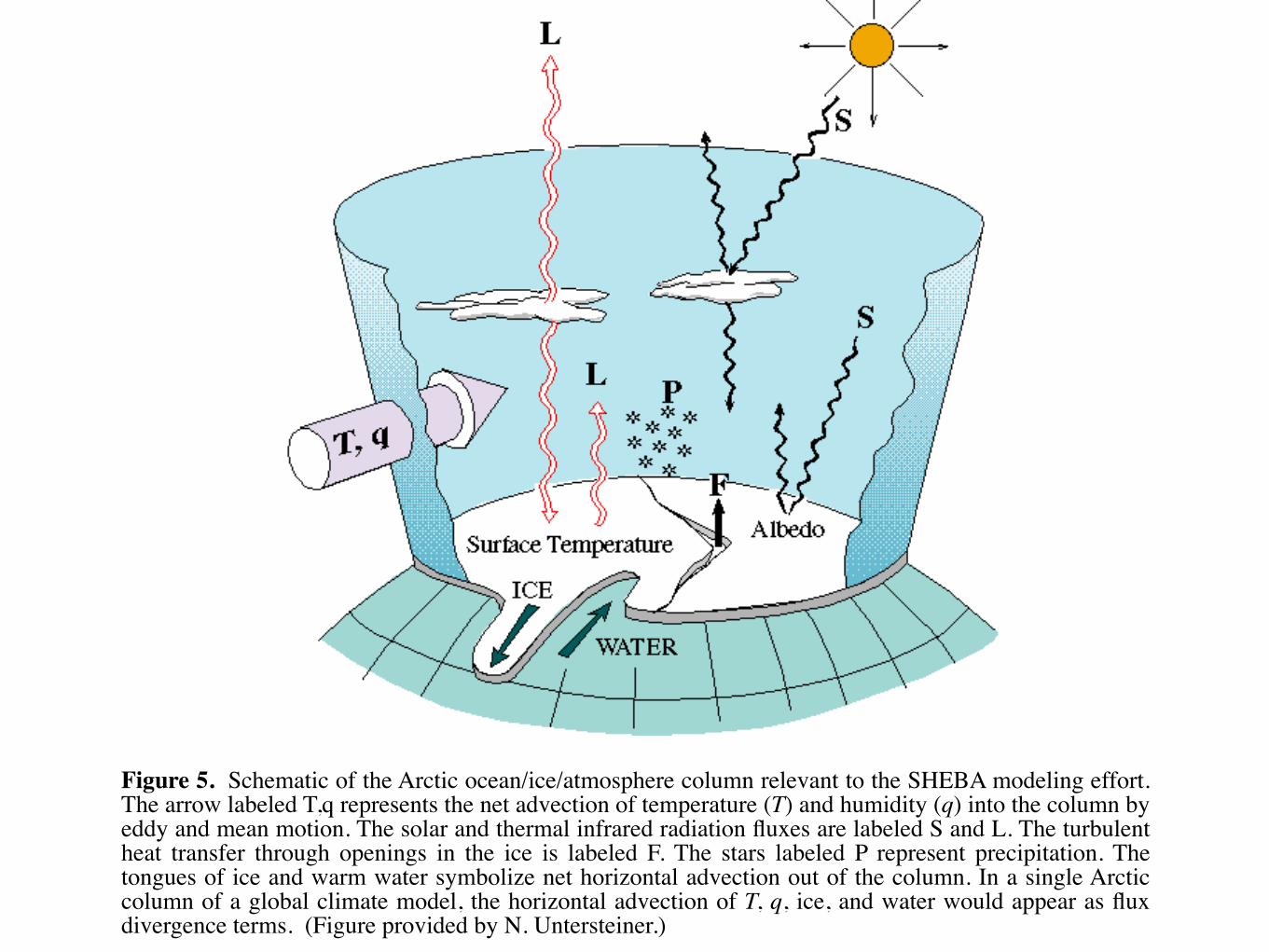
The relevant spatial scales are the diameter of the base of the column and the horizontalscales that characterize variability within the column. An upper limit on the diameter of thecolumn is set by the horizontal scale of a GCM grid cell, approximately 100–500 km. A lowerlimit on the within-column variability is set by the horizontal scale of local surface variablessuch as ice thickness, snow depth, melt pond depth, surface temperature, and surface spectralreflectance, approximately 1–1000 m. Matching the two scales requires that the within-column variability be integrated over the area in some manner. This requirement gives rise tothe concept of an aggregate spatial scale—the minimum scale at which the integratedquantities converge closely to their full column values. Since the horizontal scale of a GCMgrid cell is not determined by sea-ice properties, in principle the aggregate scale could belarger or smaller than the GCM grid cell. For at least some important variables, such asaverage ice thickness, the aggregate scale appears to be smaller than a GCM grid cell.

.

Figure 5. Schematic of the Arctic ocean/ice/atmosphere column relevant to the SHEBA modeling effort.The arrow labeled T,q represents the net advection of temperature (T) and humidity (q) into the column byeddy and mean motion. The solar and thermal infrared radiation fluxes are labeled S and L. The turbulentheat transfer through openings in the ice is labeled F. The stars labeled P represent precipitation. Thetongues of ice and warm water symbolize net horizontal advection out of the column. In a single Arcticcolumn of a global climate model, the horizontal advection of T, q, ice, and water would appear as fluxdivergence terms. (Figure provided by N. Untersteiner.)

• The “mosaic” method is commonly used in large-scale models.

• The mosaic method calculates surface fluxes over open water and sea ice surfaces using the same large-scale atmospheric profile.

• This large-scale profile is modified by these surface fluxes, using the open water (lead) fraction to specify the proportions of the over-water and sea ice fluxes.

• “Mosaic” fluxes do not depend on the lead width or orientation distributions; only the lead fraction matters.

Large-scale effects of leads: Mosaic method

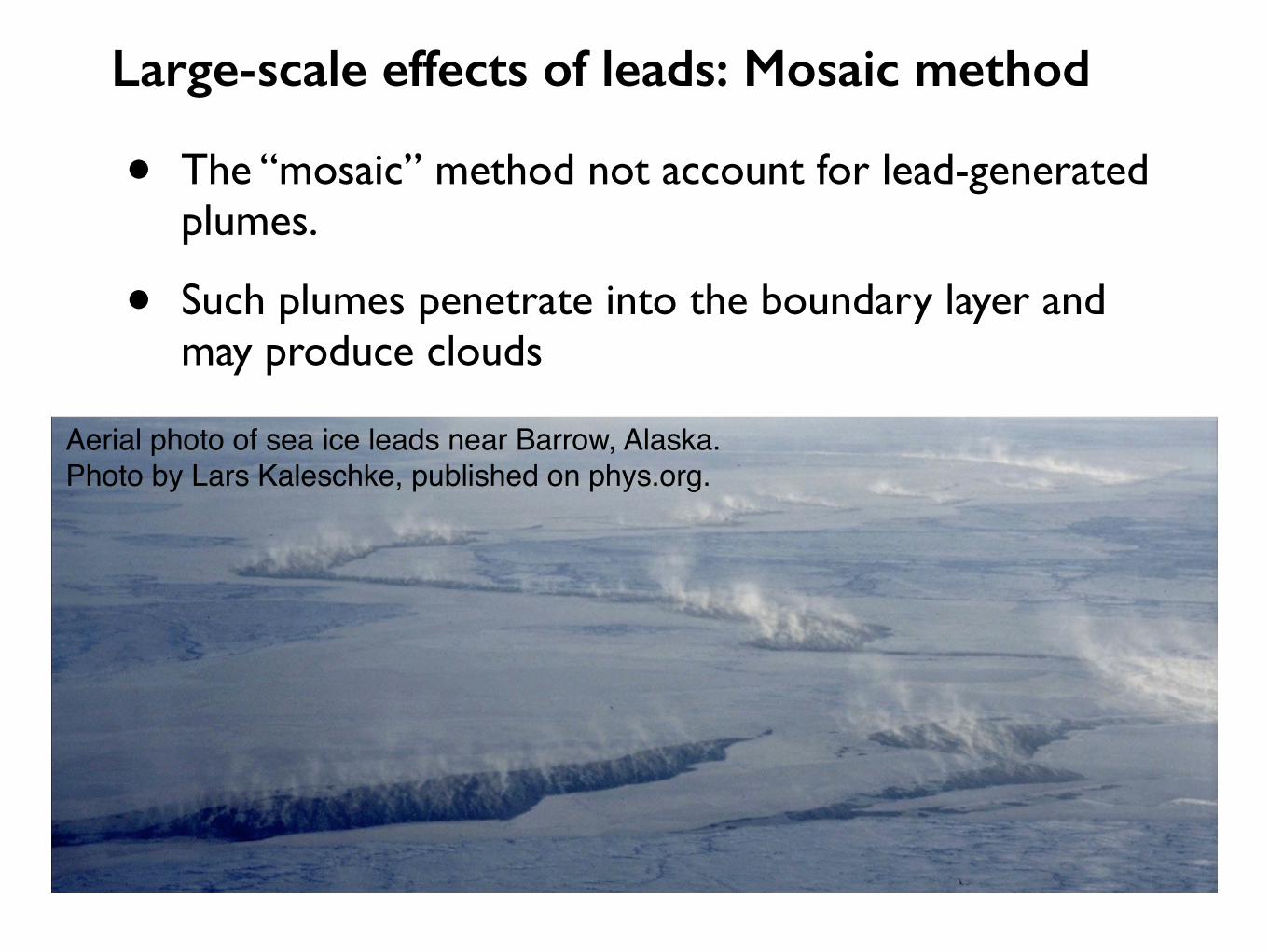
• The “mosaic” method not account for lead-generated plumes.

• Such plumes penetrate into the boundary layer and may produce clouds

Large-scale effects of leads: Mosaic method

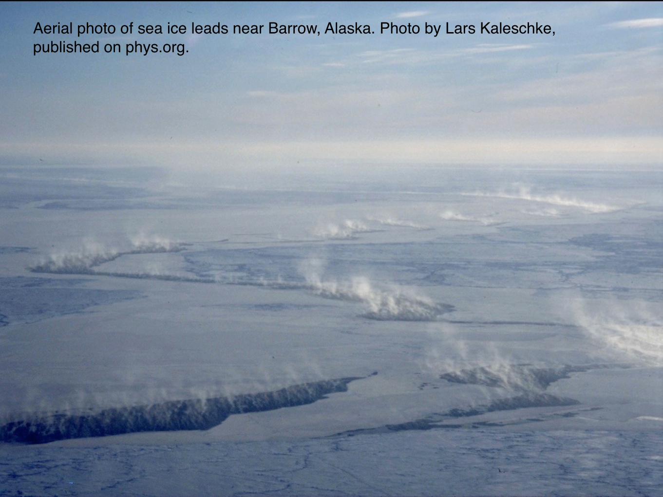
Aerial photo of sea ice leads near Barrow, Alaska. Photo by Lars Kaleschke, published on phys.org.

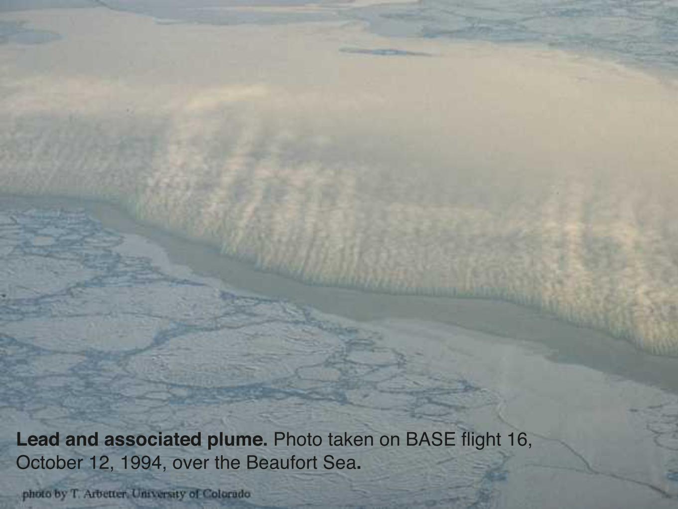
Lead and associated plume. Photo taken on BASE flight 16, October 12, 1994, over the Beaufort Sea.

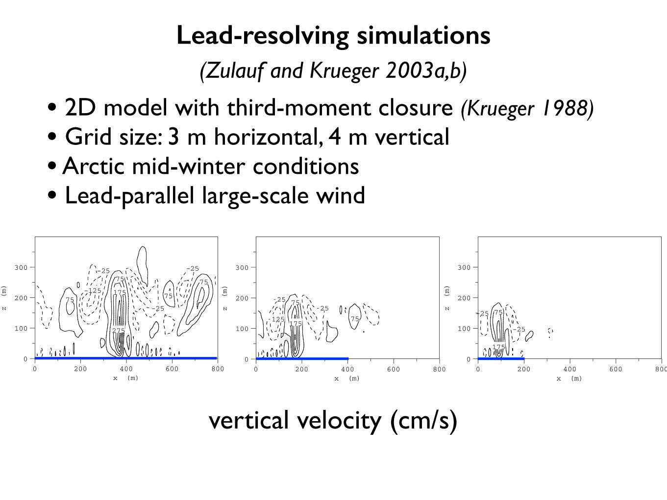
Lead-resolving simulations(Zulauf and Krueger 2003a,b)

• 2D model with third-moment closure (Krueger 1988) • Grid size: 3 m horizontal, 4 m vertical • Arctic mid-winter conditions • Lead-parallel large-scale wind

height, approximately 120 m for both the CRM and theLES. Because the bulk of the plume development does notoccur over the lead, the induced circulation does notincrease the surface fluxes as much as for the 0! case, andthey are 245 and 271 W m!2 for the CRM and the LES,respectively. Again, both models use identical resolutions: 6m in the cross-lead direction and 4 m vertically for bothmodels, and 6 m in the along-lead direction for the LES.

4. Effects of Varying Lead Width4.1. Cases Without Substantial Large-ScaleCross Wind

[22] A number of factors impact plume developmentwhen the width of the lead is varied. The primary factoris that the increased surface area for a wider lead allows fora greater total release of sensible heat to the atmosphere.The result of this may be a more vigorous circulation, and aplume that can penetrate to a greater depth.[23] The stronger circulation itself can cause a feedback

that may influence plume development. The more vigorous

circulation may manifest itself as an increase in the magni-tude of the near surface winds, leading to an increase in themagnitude of the surface fluxes. This may further intensifythe circulations, and form a positive feedback. Anothermechanism capable of increasing the near-surface windspeeds (and surface fluxes) is the vertical mixing of highermomentum air from above the surface layer down into thesurface layer, a process that is facilitated by wider leads andmore vigorous circulations. At first it may appear as if theseprocesses should have little effect; increased near-surfacewinds imply a shorter contact time between air parcels andthe warming influence of the lead surface, so to a firstapproximation individual parcels will undergo approxi-mately the same amount of heating. A larger volume of

Figure 3. Mean total vertical turbulent temperature flux(K m s!1) for a 200 m lead, 15! wind orientation, from theCRM (top, scaled by 103), and Glendening [1994, Figure 1](bottom). (Reprinted with kind permission from KluwerAcademic Publishers.)

Figure 4. Mean vertical velocity (cm s!1) for a 200 m(top), 400 m (middle), and 800 m (bottom) lead with leadparallel large-scale wind.

ZULAUF AND KRUEGER: ARCTIC LEADS AND PLUME PENETRATION HEIGHT SHE 26 - 5

















vertical velocity (cm/s)

model employs a stretched grid in the vertical direction,with an average spacing of 12 m, and a minimum spacing of4 m at the surface.[26] The most obvious feature in Figures 4–6 is that the

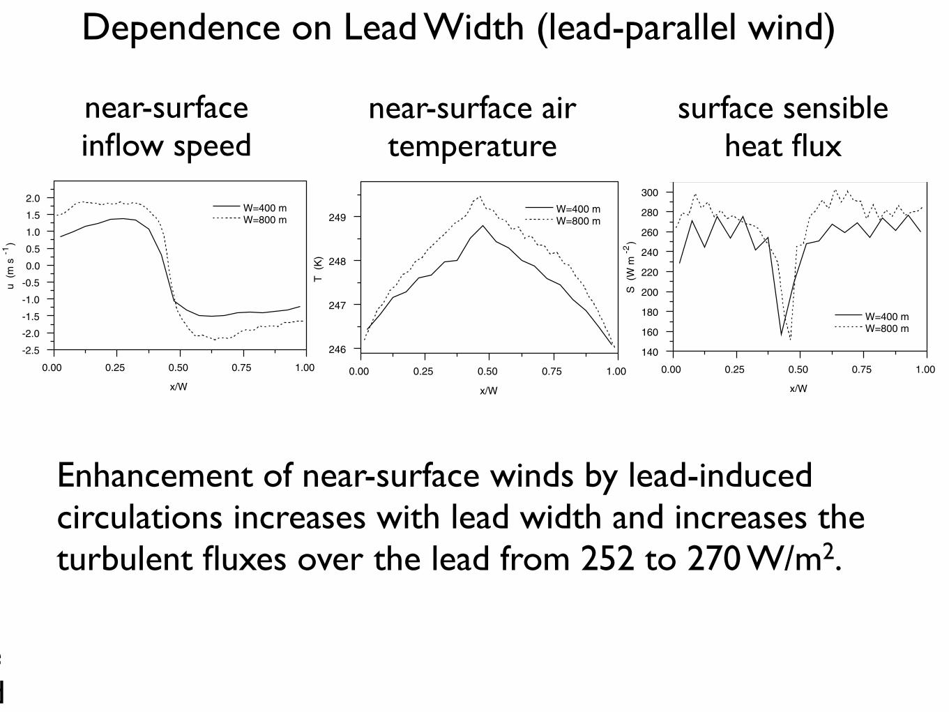
plume depth increases with increasing lead width. This is aswould be expected from the primary effect of increasedsurface area. The average surface fluxes over the leads areapproximately 256 W m!2 for the 200 m lead, 252 W m!2

for the 400 m lead, and 270 W m!2 for the 800 m lead.Further analysis illustrates that the increased air temperature

feedback decreases the sensible heat flux for the 400 m leadslightly, but then the increased strength of the circulationovercomes this negative feedback for the 800 m lead, and Sincreases noticeably. These competing feedbacks are dis-played in Figure 7, which illustrates the increases in near-surface wind speed and surface air temperatures for the 800m lead when compared with the 400 m lead. In thisinstance, the increase in near-surface wind speed is domi-nant, and the resulting surface fluxes are also increased inthe 800 m lead when compared with the narrower 400 mlead. In general, these feedbacks are relatively modest, andprobably do not influence plume development greatly at thisscale. The plumes penetrate to a depth of approximately180, 220, and 300 m for the 200, 400, and 800 m leads,respectively. As can be seen in the plots of vertical velocityand turbulent kinetic energy, the plumes that form over thewider leads are substantially more vigorous, with maximumvertical velocities increasing by approximately 1 m s!1 foreach doubling in lead width, and with similar increases seenfor the turbulent kinetic energy.

Figure 7. Comparison of near-surface inflow wind speed(top), near-surface air temperature (middle), and surfacesensible heat fluxes (bottom) as a function of fractional leadwidth for 400 and 800 m leads with lead parallel large-scalewind.

Figure 8. Mean vertical velocity (cm s!1, with 10 cm s!1

contour intervals) for a 10 km lead, no geostrophic wind,from the CRM (top), and Alam and Curry [1995, Figure 6](bottom). Alam and Curry axes labeled in km.


















Dependence on Lead Width (lead-parallel wind)

near-surface inflow speed

near-surface inflow speed

near-surface air temperature

surface sensible heat flux

Enhancement of near-surface winds by lead-induced circulations increases with lead width and increases the turbulent fluxes over the lead from 252 to 270 W/m2.

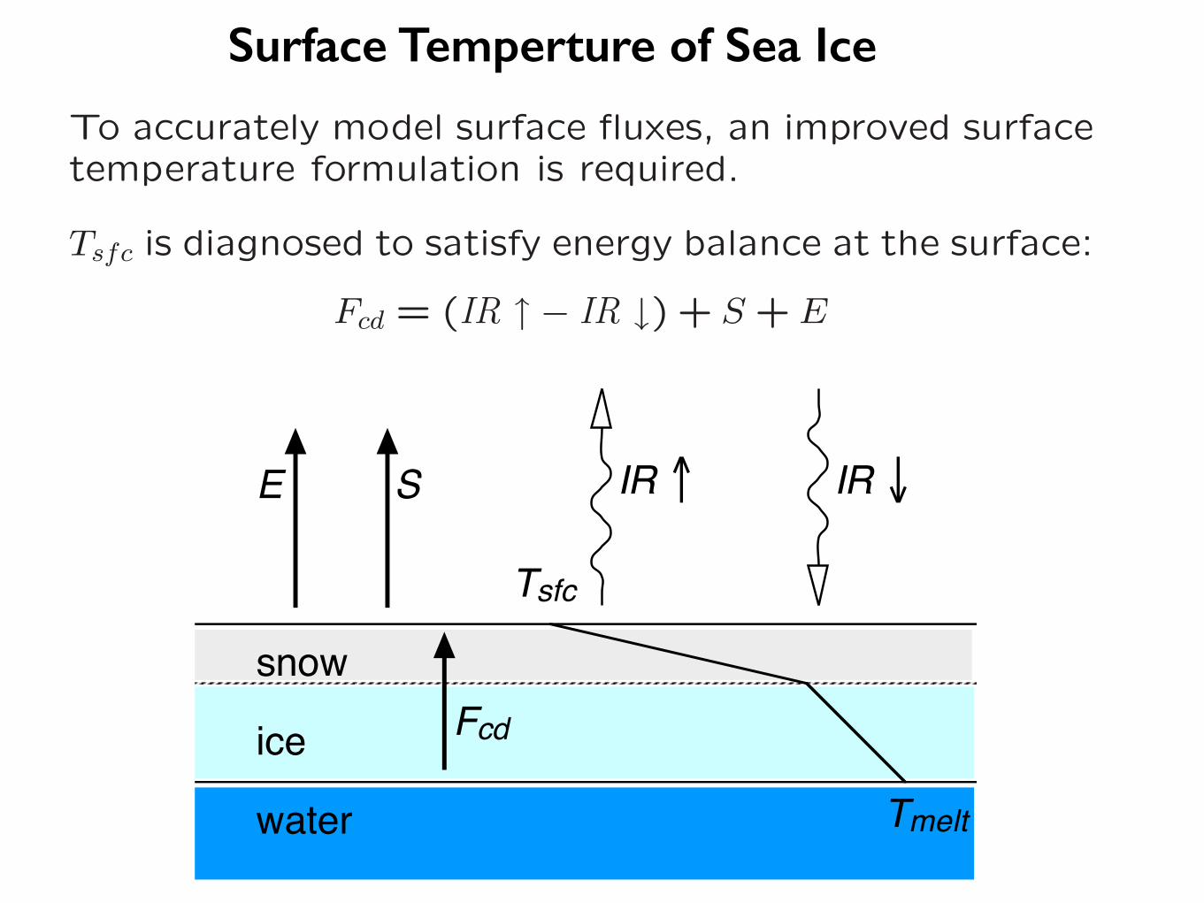
Most previous studies have handled Tsfc very simplisti-cally (ie. Tsfc held constant on snow/ice).

To accurately model surface fluxes, an improved surfacetemperature formulation is required.

Tsfc is diagnosed to satisfy energy balance at the surface:

Fcd = (IR ↑ − IR ↓) + S + E

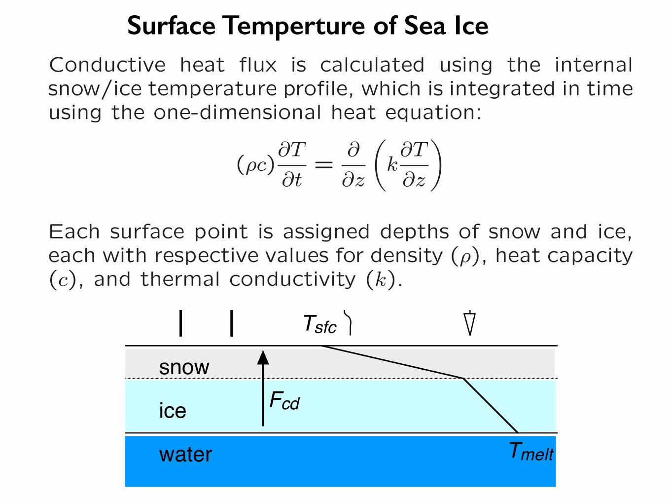
snow

ice

water

Tsfc

Tmelt

IR ! IR "E S

Fcd

Conductive heat flux is calculated using the internalsnow/ice temperature profile, which is integrated in timeusing the one-dimensional heat equation:

(ρc)∂T

∂t=

∂

∂z

!k∂T

∂z

"

Each surface point is assigned depths of snow and ice,each with respective values for density (ρ), heat capacity(c), and thermal conductivity (k).

18

Surface Temperture of Sea Ice

Surface Temperture of Sea Ice




Fcd = (IR ↑ − IR ↓) + S + E

snow

ice

water

Tsfc

Tmelt

IR ! IR "E S

Fcd


(ρc)∂T

∂t=

∂

∂z

!k∂T

∂z

"


18




Fcd = (IR ↑ − IR ↓) + S + E

snow

ice

water

Tsfc

Tmelt

IR ! IR "E S

Fcd


(ρc)∂T

∂t=

∂

∂z

!k∂T

∂z

"


18

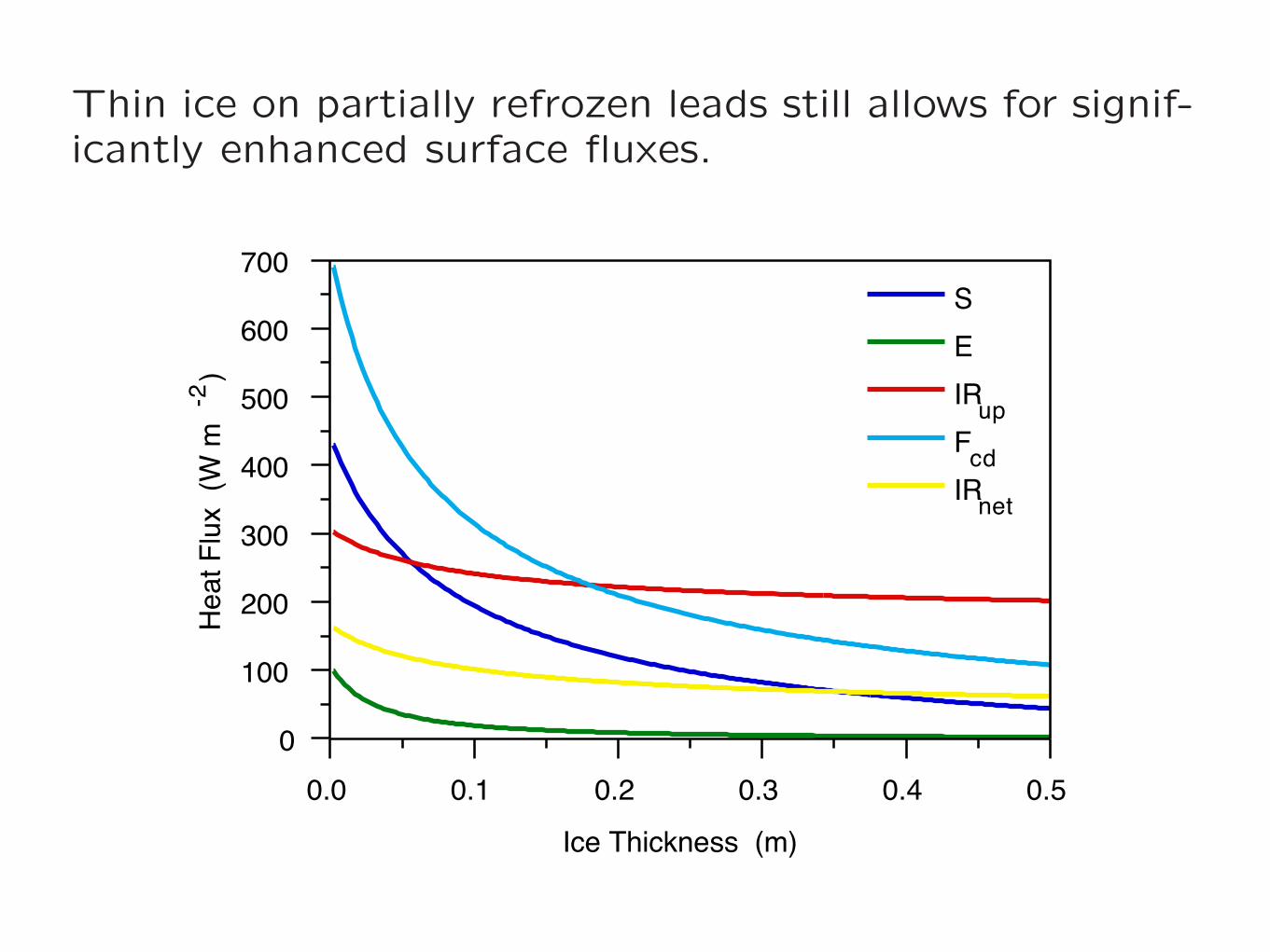
Thin ice on partially refrozen leads still allows for signif-icantly enhanced surface fluxes.

0.0 0.1 0.2 0.3 0.4 0.50

100

200

300

400

500

600

700

Ice Thickness (m)

Hea

t Flu

x (W

m-2

)

S E IRup Fcd IRnet

The parameters used in calculating this balance are:

• IR ↓ = 140 W m−2

• Tair = 240 K

• RH = 80% with respect to liquid water

• 10 m wind U = 5 m s−1

• z0 = 2 × 10−4 m

21

• Zulauf and Krueger (2003b) found that over the snow/ice portions of their simulation domains:

• the plume-induced enhancement of IR↓ increases with lead width,

• IR↑ also increases with lead width, and

• the net upward total (sensible, latent, and radiative) heat flux over the ice decreases with increasing lead width.

• Zulauf and Krueger (2003b) also found that the net upward large-scale total heat flux, Net↑, (with a lead fraction of 6.25%) increased with lead width.

Large-scale effects of single leads

-40 -35 -30 -25 -20

0

250

500

750

1000

T (degrees C)

z (m

)

observed CRM initial

40 50 60 70 80 90

RH (%)


0 5 10 15

0

250

500

750

1000

Wind Speed (m/s)

z (m

)


0 15 30 45

Wind Direction (degrees from North)


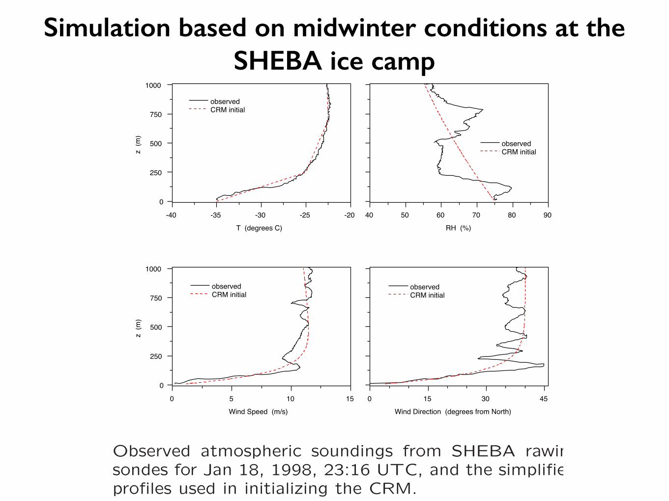
Observed atmospheric soundings from SHEBA rawin-sondes for Jan 18, 1998, 23:16 UTC, and the simplifiedprofiles used in initializing the CRM.

24

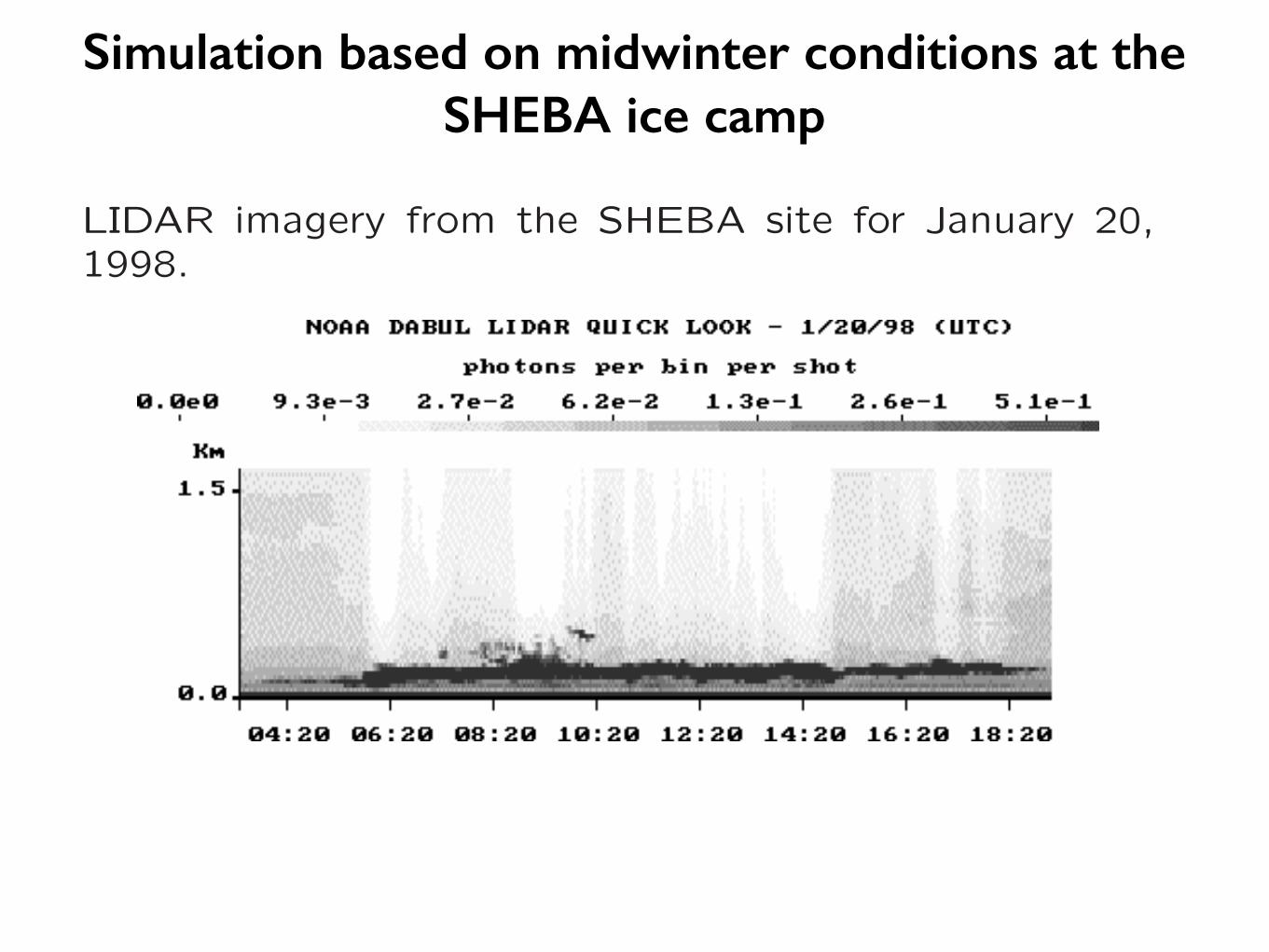
Simulation based on midwinter conditions at the SHEBA ice camp


used, 4.5 ! 10"4 m [Persson et al., 1997]. For reasons ofexpediency, we used a constant value of 1.0 ! 10"4 m overthe water surface of an open lead, rather than a fetch or sea-state-dependent value such as used by Alam and Curry[1998]. Finally, the surface temperature of the water isdefined as a constant, "2!C, because the CRM does notpresently simulate the lead freezing process.

4.2. Observations of Leads During SHEBA

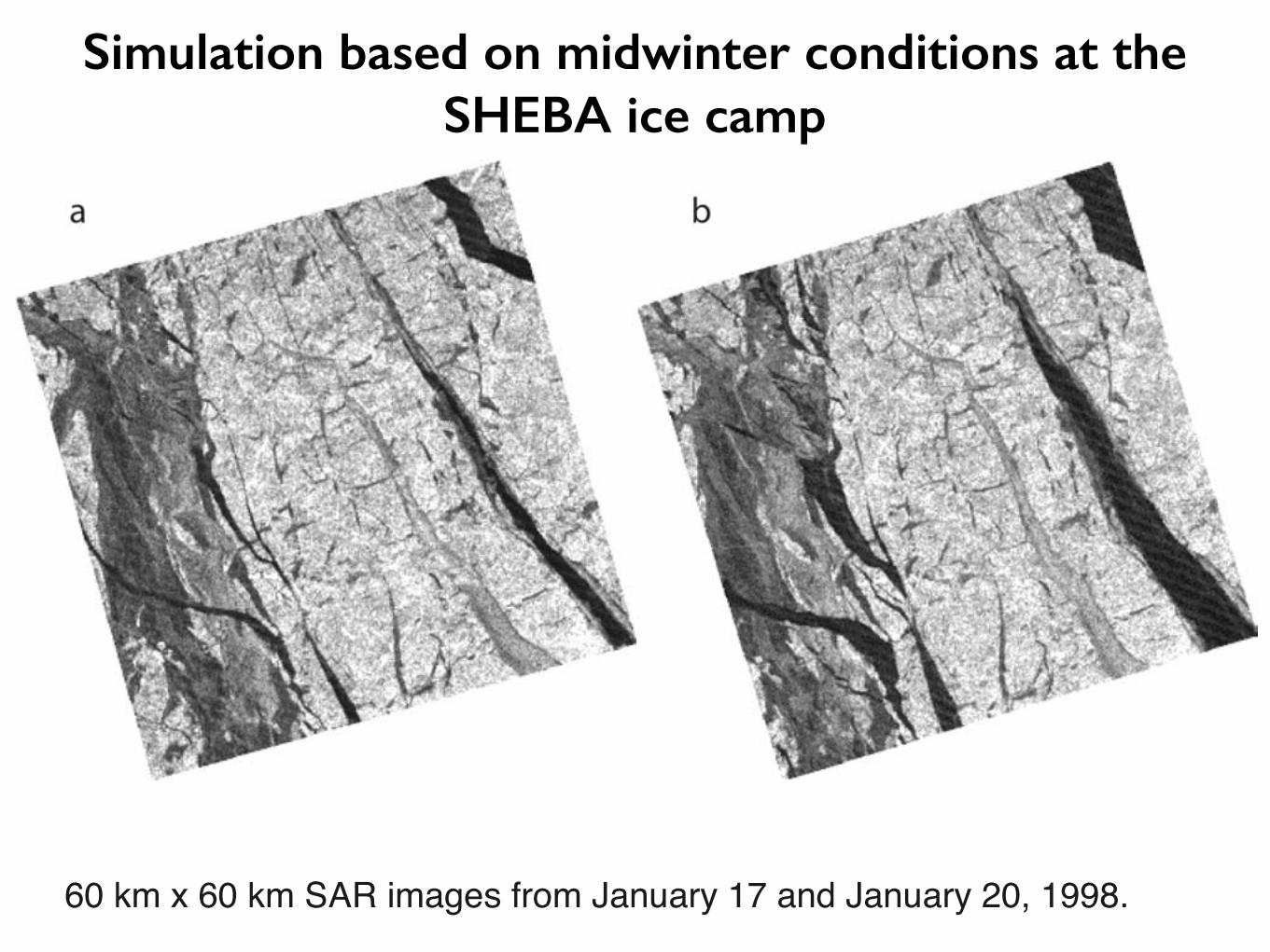
[26] Owing to the perpetual darkness of the polar winter,very few direct observations of wintertime leads are avail-able from SHEBA. The existence of leads, as well as theirsize and location, were verified, however, through the use ofvarious types of remote sensing. Very detailed images wereobtained through the use of synthetic aperture radar (SAR)(RADARSAT Images of SHEBA, distributed by H. Stern,http://psc.apl.washington.edu/Harry/Radarsat/, Copyright# 1998 by Canadian Space Agency, SAR imagery pro-cessed at the Alaska SAR Facility (Fairbanks) and distrib-uted through the SHEBA Project Office (Seattle)). Figure 4displays SAR imagery from the Canadian RADARSATsatellite for 17 January and 20 January 1998.[27] These images clearly display the opening of a large

lead approximately 15 km to the east (and approximatelyupwind based on the large-scale wind field) of the SHEBAice camp. In the second image, the lead has attained a widthof up to 8 km, though the portion directly upwind of the icecamp is closer to 3–4 km wide. In addition, other leadshave opened in the vicinity as well. Furthermore, therawinsonde data (as well as the PAM station data, etc.)show that the predominant large-scale surface wind is froma northeasterly direction, so that the near-surface air crossedthe large lead (and others nearby) nearly perpendicularlyprior to reaching the SHEBA site. Satellite IR imagery may

also be used to provide useful information of lead coverageover wide areas.[28] For atmospheric and surface conditions such as these,

it would not be surprising to see some signature of the largeleads and associated convective plumes in the observations atthe ice camp. Lidar imagery (J. Intrieri, SHEBA: LIDAR,ETL DABUL System; Quick-look PRELIMINARY datafrom Ice Camp, http://www.joss.ucar.edu/cgi-bin/codiac/dss?13.302, 1999) from 20 January (Figure 5), displays apossible consequence of the large new openings in the ice. Alow-level cloud layer was observed from approximately 0400UTC to 2000 UTC. The cloud base was typically 100 to 200m above the surface, with a thickness of up to approximately200 m. Unfortunately, owing to the localized nature of theobservations taken at the SHEBA site, it is impossible toknow for certain if these clouds are indeed related to the leadactivity.

5. Resolved Lead Simulation

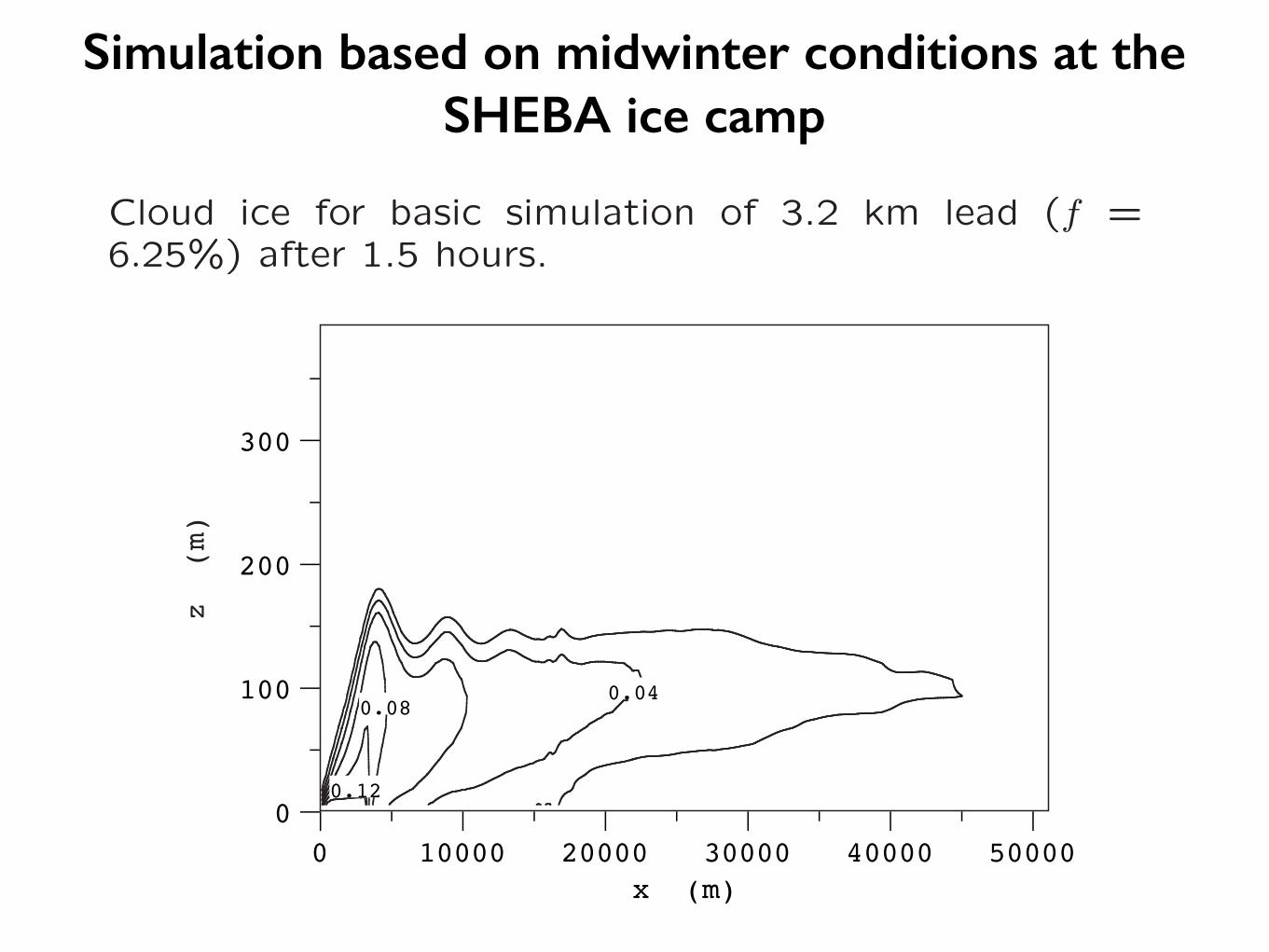
[29] On the basis of the conditions described in section 4, aseries of simulations was executed. The basic simulationfeatured a 3.2-km-wide lead in a 51.2 km domain. The leadfraction of 6.25% is larger than the average value of 1–2%,but may be more representative of the conditions during ice-divergence events such as that observed near the SHEBA icecamp around 20 January 1998. The orientation of the simu-lated lead relative to the large-scale wind field corresponds tothat of the large lead that occurred upwind of the SHEBA site.[30] Figure 6 displays vertical cross sections from the

basic simulation described above; the fields are displayed at1.5 hours and include the change from the initial conditionsin water vapor mixing ratio, the total cloud ice mixing ratio,the change in potential temperature, and the net upward IR

Figure 4. The 60 km ! 60 km SAR images from (a) 17 January and (b) 20 January 1998 (rotated sonorth is at top). The ship is at center. Note the large wedge-shaped lead several kilometers to the east.Copyright # 1998 by Canadian Space Agency.

ACL 7 - 6 ZULAUF AND KRUEGER: MODELING THE EFFECTS OF ARCTIC LEADS

60 km x 60 km SAR images from January 17 and January 20, 1998.


Cloud ice for basic simulation of 3.2 km lead (f =6.25%) after 1.5 hours.

0.12

0.080.04

0 10000 20000 30000 40000 50000

300

200

100

0

x (m)

z (m)

LIDAR imagery from the SHEBA site for January 20,1998.

25

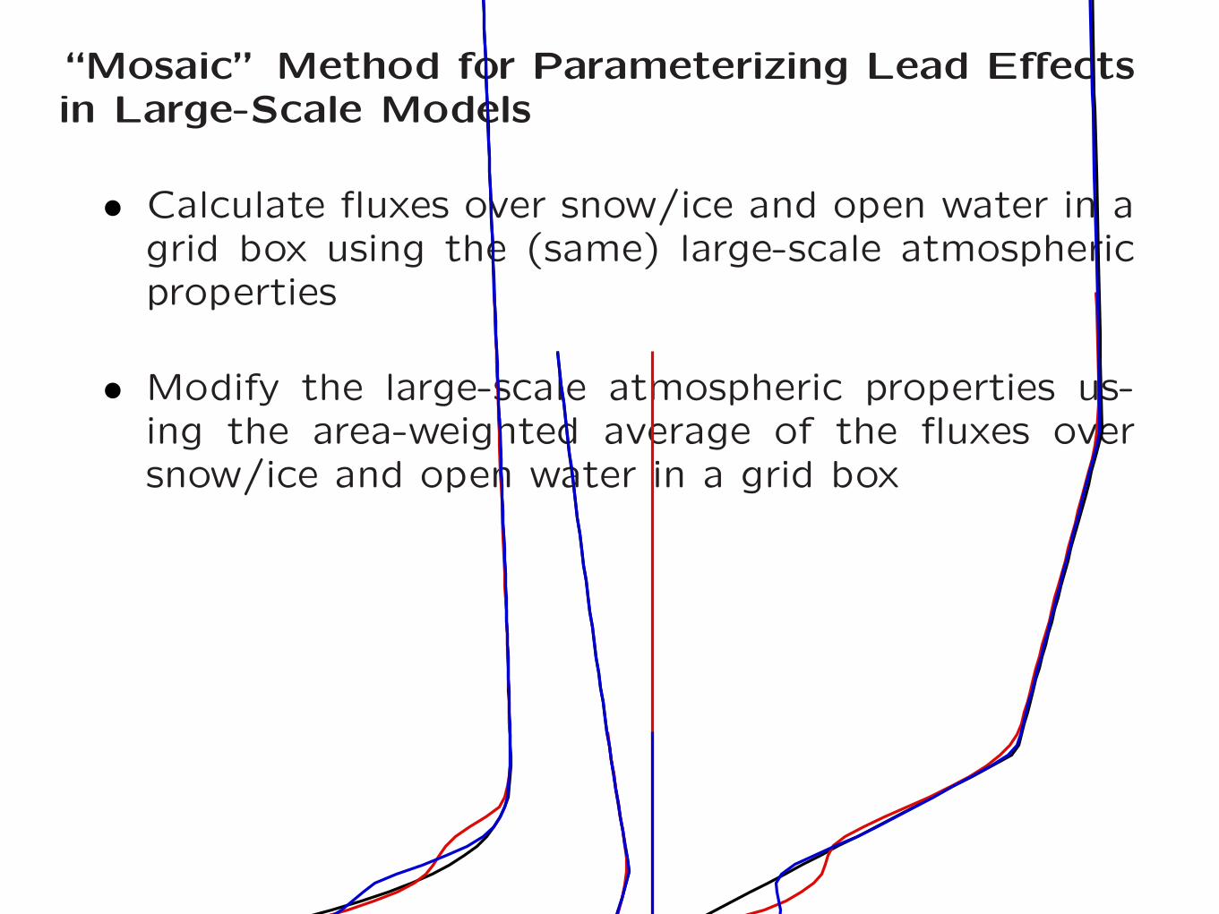
“Mosaic” Method for Parameterizing Lead Effectsin Large-Scale Models

• Calculate fluxes over snow/ice and open water in agrid box using the (same) large-scale atmosphericproperties

• Modify the large-scale atmospheric properties us-ing the area-weighted average of the fluxes oversnow/ice and open water in a grid box

0 5 10 150

100

200

300

400

wind speed (m s -1)

z (m

)

initialresolvedmosaic

240 244 248

T (K)


0.1 0.2 0.3 0.40

100

200

300

400

qv (g kg -1)

z (m

)


0.00 0.02 0.04 0.06 0.08

qi (g kg -1)

resolvedmosaic

26

Large-scale effects of leads

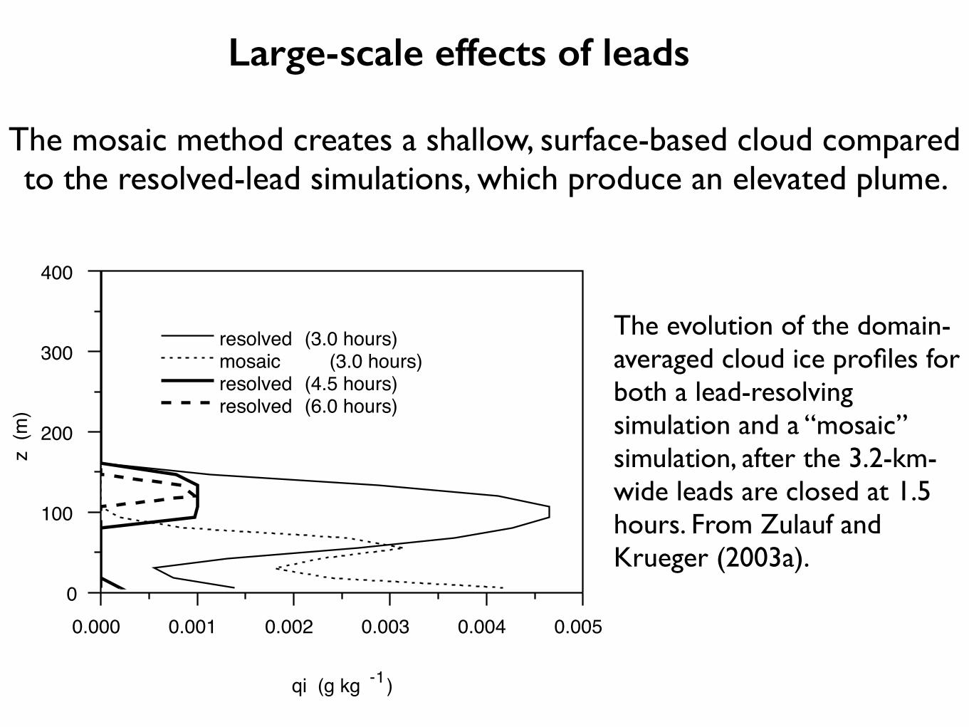
The mosaic method creates a shallow, surface-based cloud compared to the resolved-lead simulations, which produce an elevated plume.

0.000 0.001 0.002 0.003 0.004 0.0050

100

200

300

400

qi (g kg -1)

z (m

)

resolved (3.0 hours) mosaic (3.0 hours) resolved (4.5 hours) resolved (6.0 hours)

The evolution of the domain- averaged cloud ice profiles for both a lead-resolving simulation and a “mosaic” simulation, after the 3.2-km-wide leads are closed at 1.5 hours. From Zulauf and Krueger (2003a).

Large-scale effects of leads

By instantaneously spreading the heating from the lead fluxes over the snow/ice portion of the domain, the mosaic method unrealistically and significantly increases the downward turbulent sensible fluxes over the snow/ice surface compared to the resolved-lead simulations.

The lead-resolving simulations by Zulauf and Krueger (2003b) support the hypothesis that lead width is a key parameter for large leads, not just small leads, and that including a realistic estimate of the entire lead width distribution in the parameterization is important.

Large-scale effects of leadsLead-generated plumes may be conceptualized:

• (for leads oriented parallel to the large-scale surface wind direction) as convective plumes originating at a line source (the lead) that detrain at their non-buoyancy level, or

• (for leads oriented perpendicular to the wind) as plumes or thermal internal boundary layers (TIBLs) that gradually deepen downwind from the upwind lead edge.

plume are contained within the fluctuating turbulent quanti-ties, rather than the ensemble means. For both simulationsthe plume penetrates to a height of approximately 65 m. Theaverage surface sensible heat flux, S, is 244 W m!2 for theCRM, and 245 W m!2 for the LES (assuming a surface airdensity of 1.4 kg m!3). In general, the criterion used todetermine penetration height was the level at which theturbulent heat flux fell below a value of 0.5 " 10!3 K ms!1. It was found that the 0.0 K m s!1 line was often quitevariable and subject to changes in averaging time, etc. The0.5 " 10!3 K m s!1 criterion also typically agreed quitewell with other measures of plume height involving turbu-lent kinetic energy and vertical velocities.[20] A case where the wind is perpendicular to the lead

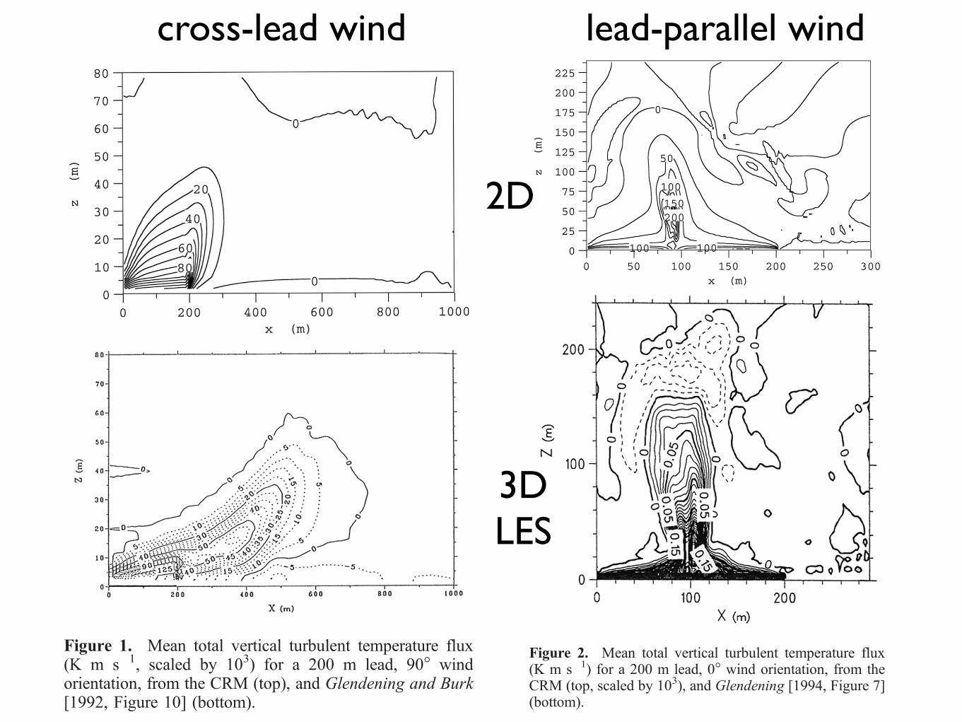
forms one extreme. The other extreme is the case where thewind is parallel to the lead, and there is no cross-leadcomponent to the large-scale geostrophic wind (f = 0!).In this instance, the convective plumes may develop directlyover the lead in an ‘‘upright’’ fashion, allowing transport ofheat to a much higher level in the inversion. Figure 2compares the vertical turbulent temperature flux obtainedby the CRM with that obtained with the LES study ofGlendening [1994] for this instance. Again, both models useidentical resolutions: 3 m in the cross-lead direction and 4 mvertically for both models, and 6 m in the along-leaddirection for the LES. The plume penetration height for

the CRM is approximately 180 m, whereas it is 160 m forthe corresponding simulation with the LES. The averagesurface sensible heat flux over the lead is 263 and 281 Wm!2 for those models, respectively. It is worth noting thatboth plumes display a slight leftward tilt, due to frictionalturning of the geostrophic forcing near the surface (theEkman spiral). It is interesting to note that the low-levelinflow to the plume acts to enhance the surface fluxes overthose seen in the f = 90! cases. For both models, the leadoccupies over half of the domain ( f = 52.1%), whichappears to have a minor impact upon the strength of theresulting circulation, as will be seen in section 4.[21] Figure 3 displays an example of an intermediate case,

when the geostrophic wind is rotated to an angle of 15! tothe lead, and the crossing time of an air parcel is approx-imately 0.9 P. Even though the crossing time is greater than0.6 P, the maximum plume development occurs near thedownwind edge of the lead. The plume shape is somewhatbetween the bent-over and upright plumes of the 90! and 0!cases. As such, the plumes penetrate to an intermediate

Figure 1. Mean total vertical turbulent temperature flux(K m s!1, scaled by 103) for a 200 m lead, 90! windorientation, from the CRM (top), and Glendening and Burk[1992, Figure 10] (bottom).

Figure 2. Mean total vertical turbulent temperature flux(K m s!1) for a 200 m lead, 0! wind orientation, from theCRM (top, scaled by 103), and Glendening [1994, Figure 7](bottom).

SHE 26 - 4 ZULAUF AND KRUEGER: ARCTIC LEADS AND PLUME PENETRATION HEIGHT

plume are contained within the fluctuating turbulent quanti-ties, rather than the ensemble means. For both simulationsthe plume penetrates to a height of approximately 65 m. Theaverage surface sensible heat flux, S, is 244 W m!2 for theCRM, and 245 W m!2 for the LES (assuming a surface airdensity of 1.4 kg m!3). In general, the criterion used todetermine penetration height was the level at which theturbulent heat flux fell below a value of 0.5 " 10!3 K ms!1. It was found that the 0.0 K m s!1 line was often quitevariable and subject to changes in averaging time, etc. The0.5 " 10!3 K m s!1 criterion also typically agreed quitewell with other measures of plume height involving turbu-lent kinetic energy and vertical velocities.[20] A case where the wind is perpendicular to the lead

forms one extreme. The other extreme is the case where thewind is parallel to the lead, and there is no cross-leadcomponent to the large-scale geostrophic wind (f = 0!).In this instance, the convective plumes may develop directlyover the lead in an ‘‘upright’’ fashion, allowing transport ofheat to a much higher level in the inversion. Figure 2compares the vertical turbulent temperature flux obtainedby the CRM with that obtained with the LES study ofGlendening [1994] for this instance. Again, both models useidentical resolutions: 3 m in the cross-lead direction and 4 mvertically for both models, and 6 m in the along-leaddirection for the LES. The plume penetration height for

the CRM is approximately 180 m, whereas it is 160 m forthe corresponding simulation with the LES. The averagesurface sensible heat flux over the lead is 263 and 281 Wm!2 for those models, respectively. It is worth noting thatboth plumes display a slight leftward tilt, due to frictionalturning of the geostrophic forcing near the surface (theEkman spiral). It is interesting to note that the low-levelinflow to the plume acts to enhance the surface fluxes overthose seen in the f = 90! cases. For both models, the leadoccupies over half of the domain ( f = 52.1%), whichappears to have a minor impact upon the strength of theresulting circulation, as will be seen in section 4.[21] Figure 3 displays an example of an intermediate case,

when the geostrophic wind is rotated to an angle of 15! tothe lead, and the crossing time of an air parcel is approx-imately 0.9 P. Even though the crossing time is greater than0.6 P, the maximum plume development occurs near thedownwind edge of the lead. The plume shape is somewhatbetween the bent-over and upright plumes of the 90! and 0!cases. As such, the plumes penetrate to an intermediate

Figure 1. Mean total vertical turbulent temperature flux(K m s!1, scaled by 103) for a 200 m lead, 90! windorientation, from the CRM (top), and Glendening and Burk[1992, Figure 10] (bottom).

Figure 2. Mean total vertical turbulent temperature flux(K m s!1) for a 200 m lead, 0! wind orientation, from theCRM (top, scaled by 103), and Glendening [1994, Figure 7](bottom).

SHE 26 - 4 ZULAUF AND KRUEGER: ARCTIC LEADS AND PLUME PENETRATION HEIGHT

3D LES

2D

cross-lead wind lead-parallel wind

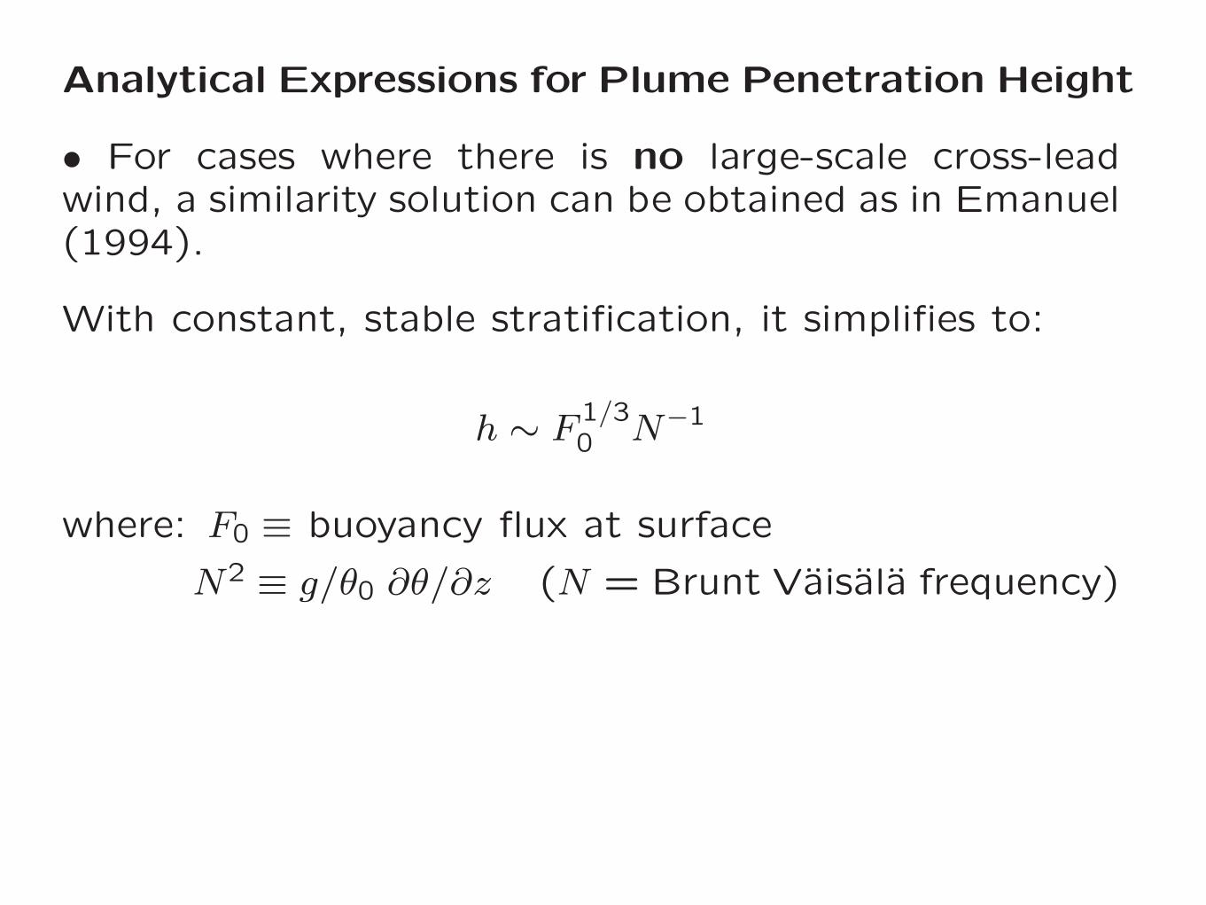
Analytical Expressions for Plume Penetration Height

• For cases where there is no large-scale cross-leadwind, a similarity solution can be obtained as in Emanuel(1994).

With constant, stable stratification, it simplifies to:

h ∼ F 1/30 N−1

where: F0 ≡ buoyancy flux at surface

N2 ≡ g/θ0 ∂θ/∂z (N = Brunt Vaisala frequency)

• For cases where there is significant large-scale cross-lead wind, Glendening and Burk (1992), using dimen-sional arguments, derived a modified expression:

h ∼ F 1/30 N−1

!W

UN

"1/3

where: W ≡ lead width

U ≡ cross-lead wind component

For case with no cross-lead wind: h ∼ W 1/3

For case with cross-lead wind: h ∼ W 2/3

10

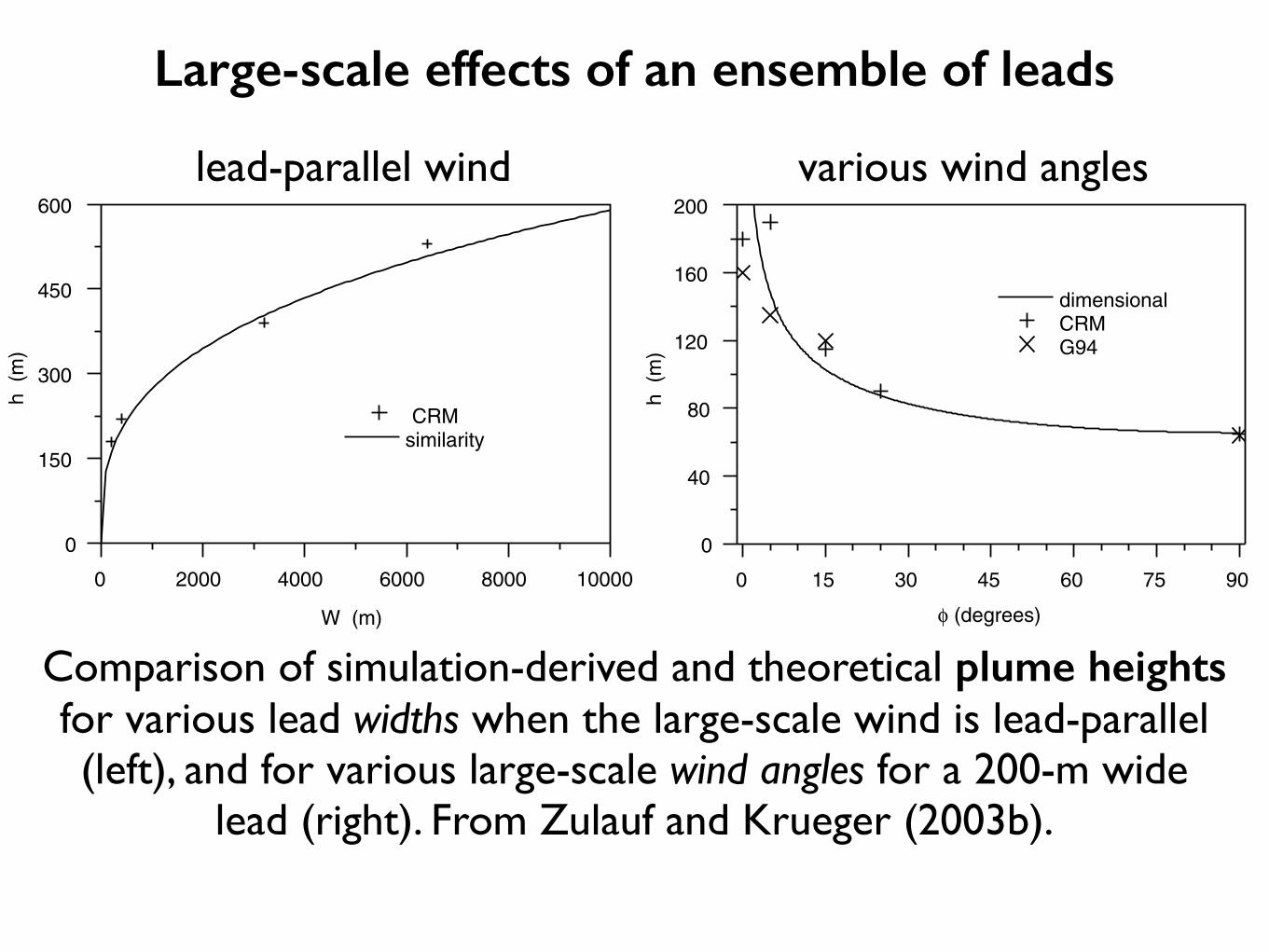
Large-scale effects of an ensemble of leads

Comparison of simulation-derived and theoretical plume heights for various lead widths when the large-scale wind is lead-parallel (left), and for various large-scale wind angles for a 200-m wide

lead (right). From Zulauf and Krueger (2003b).

of the near-surface air (a negative feedback) and increasednear-surface wind speed (a positive feedback). Theincreased near-surface wind speed appears to be due toboth the presence of a lead-scale circulation, and of verticalmixing of higher momentum air down to the surface. Forthe 3200 m lead, the increase in S is more substantial, overan 18% increase when compared with the 200 m lead,mainly due to the increased strength of the lead-inducedcirculation that forms over the wider opening. Figure 9illustrates the competition between the feedbacks as seen inboth the 1600 and 3200 m leads. Despite the substantialwarming of the near-surface air (thus lessening the air-seatemperature difference), the fluxes over the 3200 m lead aremarkedly increased when compared with the 1600 m lead,due to the increased near-surface wind speeds. Near thedownwind edge of the 3200 m lead, the wind speeds leveloff, and S begins to decrease, a consequence of the stillincreasing near-surface air temperature.

5. Comparisons With Theoretical Results

[31] For idealized cases such as are being investigatedhere, theoretical methods can provide a valuable check ofthe solutions. Following the method detailed by Emanuel[1994] for plumes emanating from a point source, a sim-ilarity solution is easily obtained for plumes emanating froma line source with no large-scale cross-wind [Zulauf, 2001].If a constant stratification is assumed, the similarity solutioncollapses to a simple expression for plume penetrationheight:

h ¼ C1F1=30 N"1; ð1Þ

where C1 is a proportionality constant, F0 is the totalbuoyancy flux of the line source, and N is the Brunt Vaisalafrequency. The total buoyancy flux may be written as

F0 ¼gWS

rq0cp; ð2Þ

where g is the acceleration of gravity, W is the lead width, Sis the average surface sensible heat flux over the lead, r is areference air density, q0 is a reference potential temperature,and cp is the specific heat of dry air at constant pressure. AsF0 varies directly with W (neglecting any changes in S dueto feedbacks), (1) dictates that h will vary with lead width asW 1/3. This type of similarity solution was first investigatedby Morton et al. [1956], and was found to show excellentagreement with laboratory experiments. It is worth reiter-ating that F0 in (1) refers to the total buoyancy released bythe lead to the atmosphere as a whole, not to individual airparcels. It is due to the effects of entrainment ofenvironmental air (a process which is included in thesimilarity solution), that one cannot simply focus on theheat that undiluted individual parcels receive.[32] As was seen in section 4.1, various feedbacks can

work to alter S with increasing lead width; this is especiallytrue for simulations in which the large-scale wind field isparallel to the lead. As a means of reducing the impact ofthese feedbacks, a series of runs were performed in whichthe surface sensible heat flux was defined as a constant, andin which there was no large-scale cross-lead wind compo-nent. Figure 10 compares the plume penetration heightsobtained by CRM simulations with those obtained by the

theoretical solution (1), for a specified surface sensible heatflux of 250 W m"2. The proportionality constant C1 hasbeen determined using the results from the initial 200 mlead. Obviously, the CRM and the similarity solution yieldexcellent agreement over a wide range of lead widths. Asubstantial difficulty remains, however, in predicting theheat flux that would occur naturally over varying widths ofleads, as the feedbacks described earlier may have asignificant impact.[33] Under realistic conditions, it is more likely that there

will be a significant cross-lead component to the large-scalewind. Obviously, in these circumstances (1) will not apply.Glendening and Burk [1992] developed an expression toaccount for cross-lead winds, based upon the earlier work ofTurner [1973]. This expression employs dimensional argu-ments, and is a modification of (1) that contains the ratiobetween the advective time scale of the lead (W/U ) and thebuoyancy time scale (N"1) of the atmosphere, where U isthe cross-lead component of the large-scale wind:

h ¼ C2F1=30 N"1 W

UN

! "1=3

; ð3Þ

where C2 is another proportionality constant, which wasdetermined by Glendening and Burk [1992] to beapproximately unity, based on their results from LES. Aninteresting point is that plume height for leads with nocross-wind varies with W 1/3 holding other parametersconstant, but for cases with a cross-wind, (3) predicts thatplume height should vary as W 2/3 (since F0 varies directlywith W ). Furthermore, when the dimensional solutionproposed by Glendening and Burk [1992] is written in theform shown in (3), it becomes unclear why the dimension-less W

U N# $

term should be raised to the 1/3 power. In adimensional sense this exponent appears to be arbitrary.[34] As was done in section 3, by holding the lead width

constant and varying the direction of the large-scale wind,the response of plume height to changes in the strength ofthe cross-lead component of wind can be tested. Since thesurface fluxes were not seen to vary too greatly for a 200 m

Figure 10. Comparison of CRM derived plume penetra-tion heights with theoretical solution for cases withspecified surface fluxes, varying lead width, and no large-scale cross-wind.


lead with varying wind direction, fluxes were calculatedusing the standard formulation, rather than specified as forthe previous example. Figure 11 compares results from theCRM with LES results of Glendening [1994] and theexpression given by (3). One problem with (3) is readilyapparent in the way that the predicted plume heightapproaches infinity at low wind angles, where (1) shouldbe more applicable. For angles greater than approximately10!, the dimensional solution shows good agreement withboth CRM and LES results, which also show good agree-ment with each other.[35] The question remains whether the W 2/3 dependence

of plume height predicted by (3) is accurate. To address thisissue, Figure 12 compares results from the CRM with thedimensional solution predicted by (3) for increasing leadwidth. The CRM results are those that were tabulated inTable 1. Again, as S was not greatly affected by increasinglead width, fluxes were calculated in the standard fashion. Itis clear from Figure 12 that the results from the CRM and(3) diverge rapidly as the lead width increases. Burk et al.[1997] obtained similar results using their two-dimensionalsteady-state boundary layer model. These results seem toput some doubt on the validity of (3) and theW 2/3 scaling ofplume heights when there are significant cross-lead winds.It is possible, however, that the dependence of plumepenetration height upon lead width may differ dependingupon the ratio of lead crossing and the buoyant responsetimes. Assuming we include the effects of entrainment, thisratio may be written as

R ¼ W

U

! "

= 0:6Pð Þ: ð4Þ

For R < 1, the plume is of the bent-over type, while for R >1 the resulting plume is more upright. Under the simulatedconditions, the R = 1 dividing line occurs at a lead width ofapproximately 500 m. Although it is difficult to sayconclusively based only upon the three lead widthscorresponding to R < 1, it still appears as if the CRMresults diverge from the solution proposed in (3); thedimensional expression underpredicts the plume height for

the 100 m lead, but overpredicts the height for the 400 mlead. For the lead widths corresponding with R > 1 thediscrepancy between the analytical expression and CRMresults is much more obvious.[36] Included in Figure 12 is a line displaying a W 1/2

scaling for plume penetration height, which appears to yielda much better fit for the CRM results. Whereas there hasbeen significant work studying the behavior of point-sourceplumes in the presence of cross flows [e.g., Lavelle, 1997]),there has been relatively little work studying the behavior offinite width line-source plumes under the same conditions.Unfortunately, it appears to be very difficult to translate thefindings relevant to point source plumes to finite width linesource plumes. On the other hand, the W1/3 scaling for thecase where there is no large-scale cross-lead wind, which isbased upon the more robust foundation of a similaritysolution, seems to hold true for both numerical simulationsand laboratory experiments.

6. Effects of Additional Physics

[37] For reasons of computational efficiency or modelcomplexity, many studies modeling the impacts of leadinduced plumes have neglected microphysical and radiativeprocesses. Burk et al. [1997] did include these effects intheir study, but did not conduct sensitivity experiments todetermine their relative importance. Pinto et al. [1995] didinvestigate these sensitivities, but their model was one-dimensional, and did not resolve the circulations that candevelop when both ice and water surfaces are present.Instead, their study examined the development of a thermalinternal boundary layer as profiles of cold air were advectedover very wide, open leads.[38] For the most part, the omission of these processes is

a valid simplification, because at the temperatures and timescales of interest, sensible heating is thought to be thedominant process. Nonetheless, these other processes needto be investigated, especially since the addition of moistureto the Arctic atmosphere is of primary interest. As we arepresently interested in the Arctic winter, solar radiation neednot be considered.

Figure 11. Comparison of CRM and LES [from Glenden-ing, 1994] (labeled as G94) derived plume penetrationheights with theoretical solution for cases with naturalfluxes and varying large-scale wind angle.

Figure 12. Comparison of CRM derived plume penetra-tion heights with theoretical solution for cases with naturalfluxes, varying lead width, and large-scale cross-wind.Included in the plot is the improved W 1/2 scaling.

SHE 26 - 10 ZULAUF AND KRUEGER: ARCTIC LEADS AND PLUME PENETRATION HEIGHTlead-parallel wind various wind angles

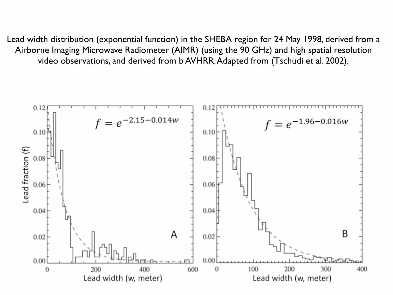
Lead width distribution (exponential function) in the SHEBA region for 24 May 1998, derived from a Airborne Imaging Microwave Radiometer (AIMR) (using the 90 GHz) and high spatial resolution

video observations, and derived from b AVHRR. Adapted from (Tschudi et al. 2002).

Large-scale effects of an ensemble of leadsSTRONG: Parameterizing e�ects of leads 15

Mass Flux (kg m−2 s−1)

Hei

ght (

m)

Mass Flux per unit lead area

0 2 4 60

100

200

300

400

50025% (1−1.2 m)50% (1−1.7 m)75% (1−2.8 m)All Leads (1−10 m)

Detrainment Rate (kg m−3 s−1)

Hei

ght (

m)

Detrainment Rate per unit lead area

0 0.1 0.2 0.3 0.40

100

200

300

400

500All Leads (1−10 m)

Mass Flux (kg m−2 s−1)

Hei

ght (

m)

Mass Flux per unit lead area

0 0.5 1 1.50

100

200

300

400

50025% (10−12.9 m)50% (10−18.6 m)75% (10−34.8 m)All Leads (10−2000 m)

Detrainment Rate (kg m−3 s−1)

Hei

ght (

m)

Detrainment Rate per unit lead area

0 0.01 0.02 0.03 0.040

100

200

300

400

500All Leads (10−2000 m)

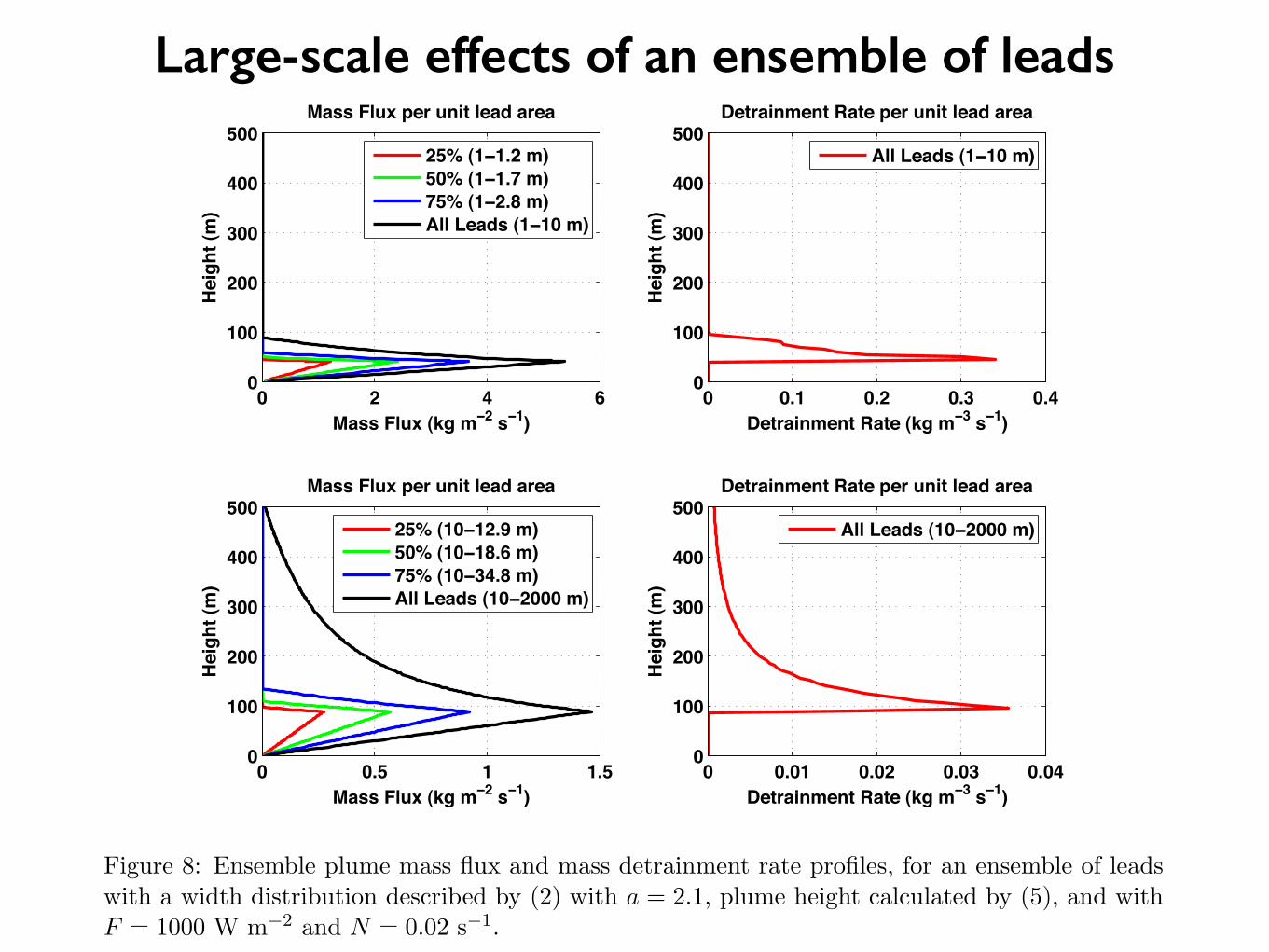
Figure 8: Ensemble plume mass flux and mass detrainment rate profiles, for an ensemble of leadswith a width distribution described by (2) with a = 2.1, plume height calculated by (5), and withF = 1000 W m�2 and N = 0.02 s�1.

winds originates over the downstream edge of the lead (Fig. 1 of Zulauf and Krueger (2003b)).The results presented in Zulauf and Krueger (2003b)) suggest that plume-base properties can beparameterized as functions of lead width, lead orientation, a fetch-dependent surface flux, andatmospheric stability. We will combine TIBL theory and lead-resolving simulations to producesuch a parameterization.

A fraction of the condensate may precipitate near the lead, while the remainder will be detrainedto the large-scale environment. Lead-resolving simulations will provide guidance for parameterizingthis source of large-scale condensate, but there will be uncertainties due to the ice microphysicsparameterizations (see section 10). These uncertainties have been significantly reduced over the past10 years by three major model intercomparison projects led by the GCSS (GEWEX Cloud SystemStudy) WG 5 (Polar Clouds) working group and by ARM (Atmospheric Radiation Measurementprogram) for well-observed Arctic cloud systems (see section 10).

The large-scale heating and moistening e�ects due to the penetrating convective plumes arisenot only from detrainment, but also from plume-induced subsidence in the environment (Arakawaand Schubert 1974). For example, the tendency of the large-scale potential temperature, �, due toplume-induced subsidence is M⌅�/⌅z, where M is the ensemble plume mass flux calculated from(7) and the frequency distribution of lead widths given by (2).

A simple yet general approach to including the ensemble e�ects of a realistic lead distribution,

• Alam and Curry (1997), Andreas and Cash (1999), and Marcq and Weiss (2012) suggest that the average or integrated surface fluxes over a lead depend on fetch (i.e., on lead width and orientation).

• Alam (2000) included a fetch dependence in her parameterization of the grid-averaged surface fluxes. However, Alam did not include the effects of lead-generated circulations found by Zulauf and Krueger (2003a,b).

Parameterizing lead-scale processes and their large-scale effects

• Lead width distribution: negative expontial or power law

• Lead orientation distribution: assumes that the ice floe and lead orientation distributions are related

Analysis and parameterization of lead geometry

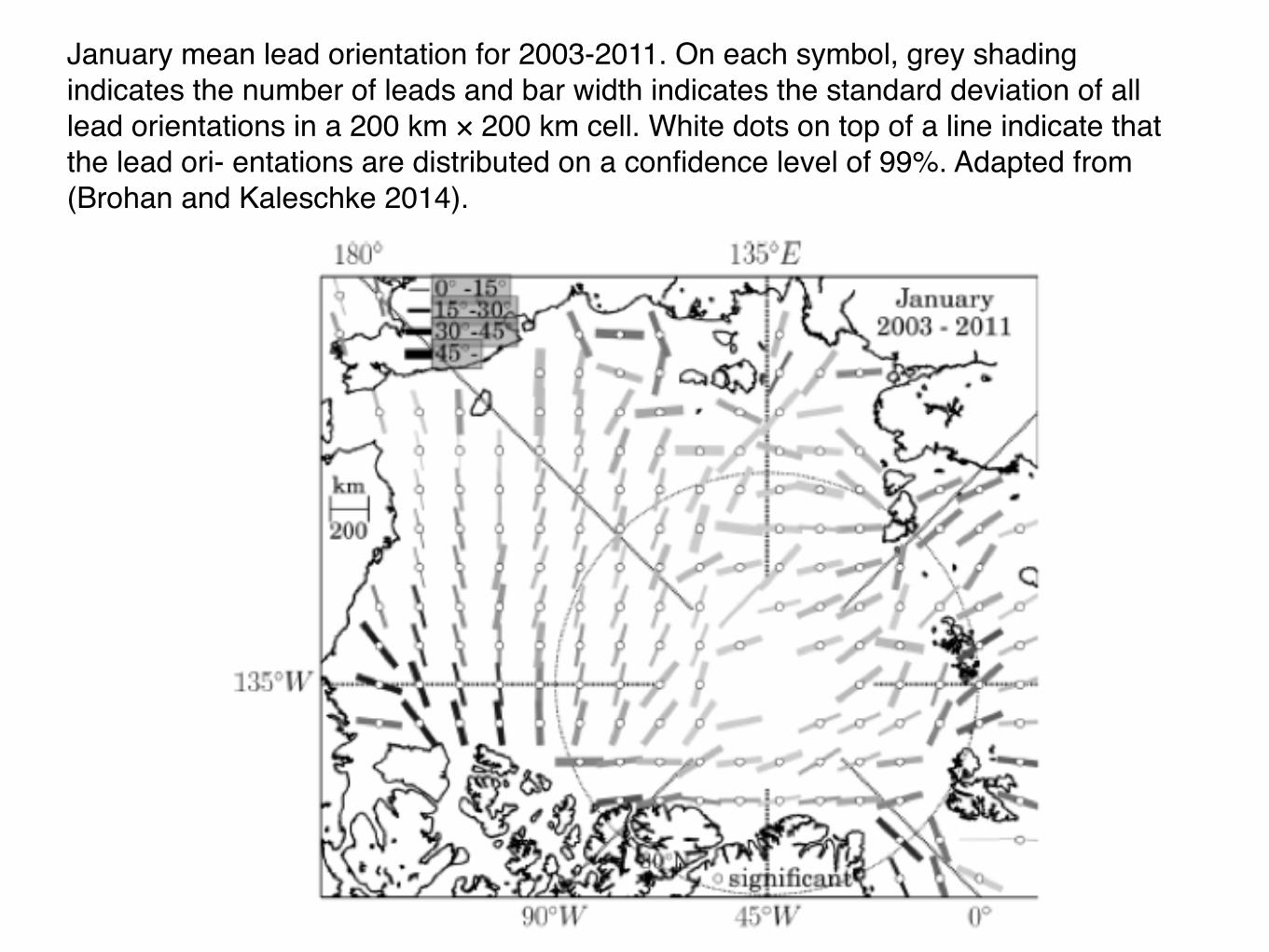
January mean lead orientation for 2003-2011. On each symbol, grey shading indicates the number of leads and bar width indicates the standard deviation of all lead orientations in a 200 km × 200 km cell. White dots on top of a line indicate that the lead orientations are distributed on a confidence level of 99%. Adapted from (Brohan and Kaleschke 2014).

Summary

• Arctic leads produce significant fluxes of heat and water vapor into the atmosphere.

• Lead-generated plumes can penetrate into the boundary layer and produce elevated cloud layers.

• Plume properties can be parameterized given lead width and orientation.

• Lead width and orientation distributions can be now be parameterized.

• The large-scale effects of an ensemble of leads could be parameterized more realistically than by using the mosaic method.

Aerial photo of sea ice leads near Barrow, Alaska. Photo by Lars Kaleschke, published on phys.org.

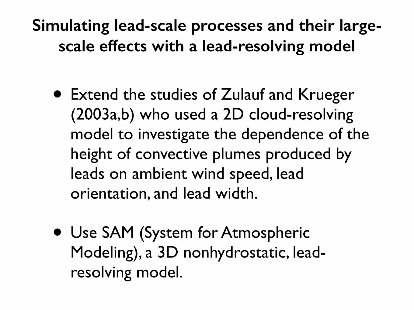
• Extend the studies of Zulauf and Krueger (2003a,b) who used a 2D cloud-resolving model to investigate the dependence of the height of convective plumes produced by leads on ambient wind speed, lead orientation, and lead width.

• Use SAM (System for Atmospheric Modeling), a 3D nonhydrostatic, lead-resolving model.

Simulating lead-scale processes and their large-scale effects with a lead-resolving model

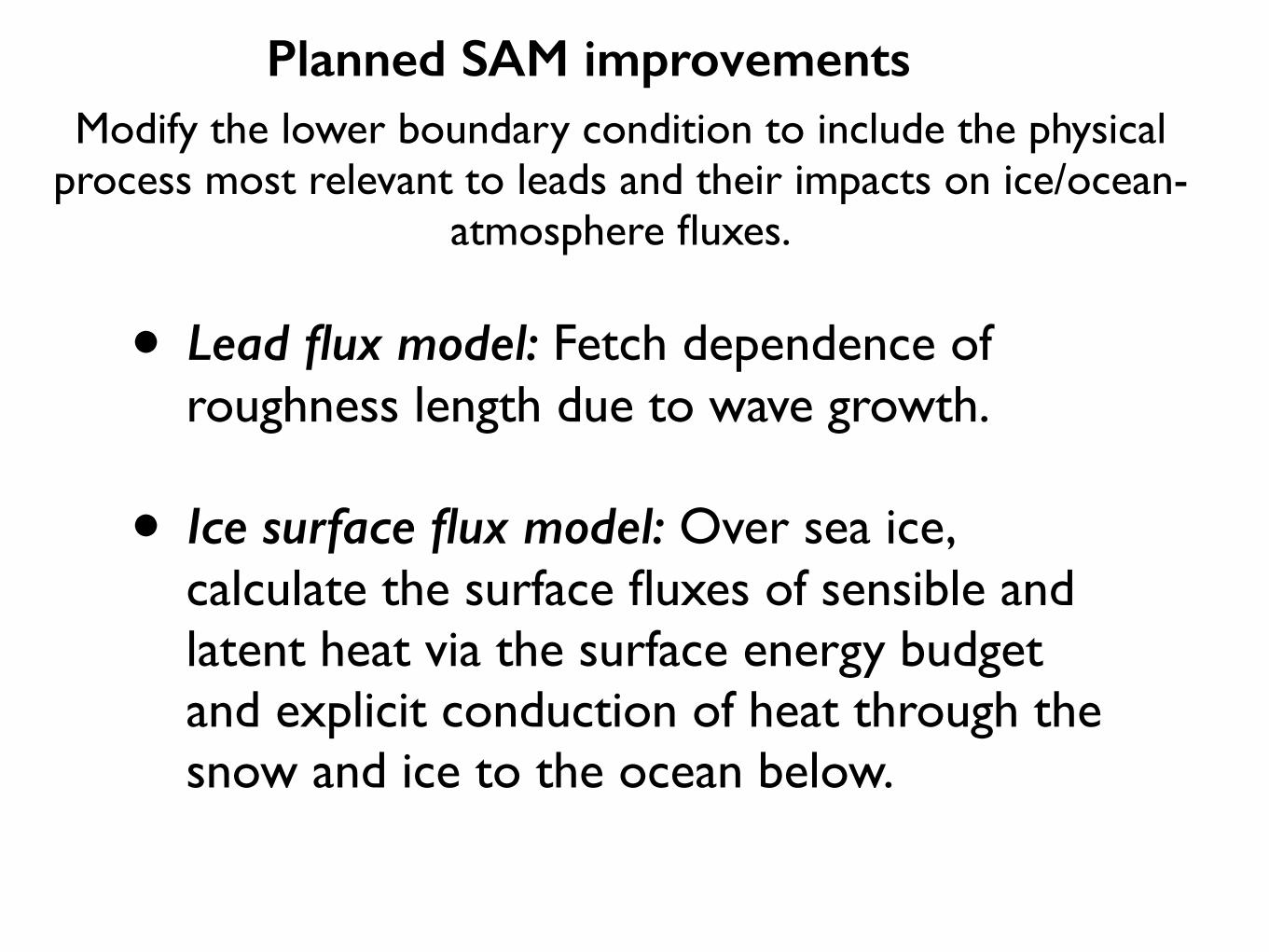
• Lead flux model: Fetch dependence of roughness length due to wave growth.

• Ice surface flux model: Over sea ice, calculate the surface fluxes of sensible and latent heat via the surface energy budget and explicit conduction of heat through the snow and ice to the ocean below.

Planned SAM improvementsModify the lower boundary condition to include the physical

process most relevant to leads and their impacts on ice/ocean-atmosphere fluxes.

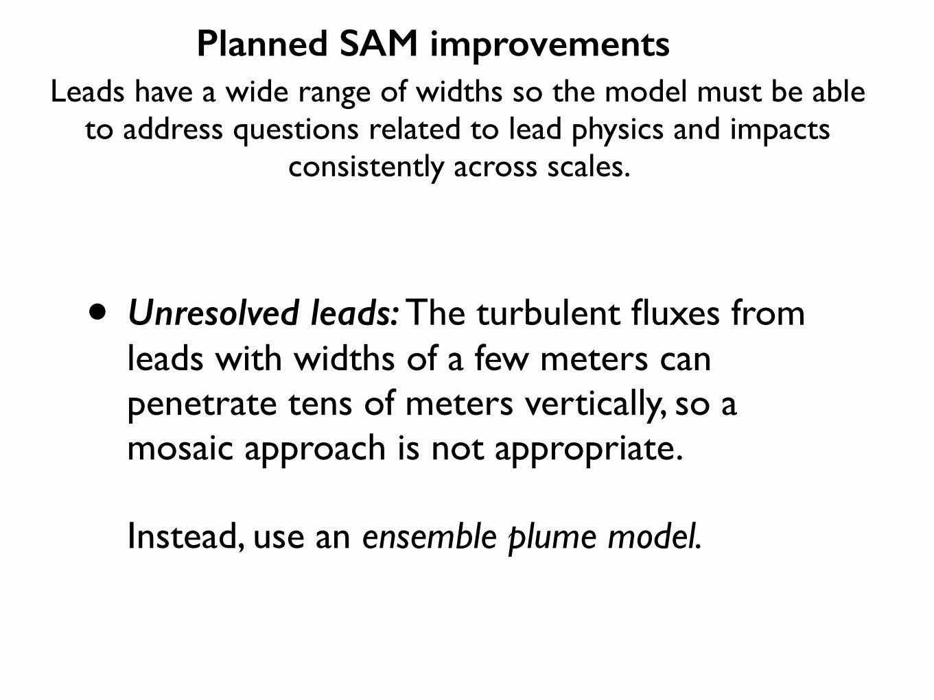
• Unresolved leads: The turbulent fluxes from leads with widths of a few meters can penetrate tens of meters vertically, so a mosaic approach is not appropriate.

Instead, use an ensemble plume model.

Planned SAM improvementsLeads have a wide range of widths so the model must be able

to address questions related to lead physics and impacts consistently across scales.

Lead-Resolving Simulations

The modified version of SAM will be used to perform a series of lead-resolving simulations to:

• develop an understanding of the key mechanisms that govern ice-lead-atmosphere interactions in the Arctic

• extend our knowledge of the properties and large-scale effects of lead-induced plumes.

[add graphic]

• Limited domain idealized simulations over small leads

• Large domain idealized simulations over leads

• Large domain simulations with realistic lead width distributions

Lead-Resolving SimulationsWe will use three basic types of simulations:

• Limited domain idealized simulations over small leads

• We will explore the interaction between multiple small leads (as the most prevalent, they are the most likely to be in proximity of each other), the impact of incident wind direction on lead fluxes of heat and water vapor, and the impact of background atmospheric stability.

• Use grid sizes as small as ≈ 1 m and domains up to 2 km in extent.


• Large domain idealized simulations over larger leads

• We will test existing and new parameterizations for lead-induced fluxes in climate simulations

• Use a 50 km x 50 km domain and a grid size of 25 m.


• Large domain simulations with realistic lead width and orientation distributions

• Our analysis of this set of simulations will focus on lead-plume interactions and their impact and feedback with local atmospheric conditions through enhanced cloud formation and radiative feedback mechanisms.

• The horizontally averaged fluxes will provide benchmarks to evaluate existing and new CESM winter Arctic ice flux parameterization models.


parameterizing the effects of leads upon the atmosphere ... · parameterizing the effects of leads...

Documents