PARAMETER ESTIMATION IN MERTON JUMP DIFFUSION MODEL

A THESIS SUBMITTED TOTHE GRADUATE SCHOOL OF NATURAL AND APPLIED SCIENCES

OFMIDDLE EAST TECHNICAL UNIVERSITY

BY

TUGCAN ADEM ÖZDEMIR

IN PARTIAL FULFILLMENT OF THE REQUIREMENTSFOR

THE DEGREE OF MASTER OF SCIENCEIN

STATISTICS

JULY 2019

Approval of the thesis:

PARAMETER ESTIMATION IN MERTON JUMP DIFFUSION MODEL

submitted by TUGCAN ADEM ÖZDEMIR in partial fulfillment of the require-ments for the degree of Master of Science in Statistics Department, Middle EastTechnical University by,

Prof. Dr. Halil KalıpçılarDean, Graduate School of Natural and Applied Sciences

Prof. Dr. Aysen Dener AkkayaHead of Department, Statistics

Assist. Prof. Dr. Ceren Vardar AcarSupervisor, Statistics Department, METU

Examining Committee Members:

Assist. Prof. Dr. Fulya Gökalp YavuzStatistics Department, METU

Assist. Prof. Dr. Ceren Vardar AcarStatistics Department, METU

Assoc. Prof. Dr. Aslı YıldızMathematics Department, Hacettepe University

Date:

I hereby declare that all information in this document has been obtained andpresented in accordance with academic rules and ethical conduct. I also declarethat, as required by these rules and conduct, I have fully cited and referenced allmaterial and results that are not original to this work.

Name, Surname: Tugcan Adem Özdemir

Signature :

iv

ABSTRACT

PARAMETER ESTIMATION IN MERTON JUMP DIFFUSION MODEL

Özdemir, Tugcan Adem

M.S., Department of Statistics

Supervisor: Assist. Prof. Dr. Ceren Vardar Acar

July 2019, 84 pages

Over the years, jump diffusion models become more and more important. They are

used for many purposes in several branches such as economics, biology, chemistry,

physics, and social sciences. The reason for prevalent usage of these jump models

is that they capture stochastic movements and they are sensitive to jump points. It is

possible to measure sudden decreases/increases caused by some reasons such as wars,

natural disasters, market crashes or some dramatic news, by jump diffusion models.

Recently, US Dollar to Turkish Lira exchange rate has showed dramatic increases/de-

creases. It is very difficult to model this exchange rate data with classical modeling

methods. In this thesis, we try to model this data with Merton model which is among

the well-known jump diffusion models. To obtain true parameter estimation algo-

rithm, we simulate a data by using Merton structure. The values of parameters are

found with Maximum Likelihood Estimation (MLE). The initial parameter values in

simulated data and the estimated parameter values are compared to control the pa-

rameter estimation is true or not. Also, the values of Euler-Maruyama numerical ap-

proximation method and analytical solution values are checked whether convergence

v

is good or not. After the true parameter estimation algorithm is found, US Dollar

to Turkish Lira exchange rate data is used. This data is between date of 01.02.2019

and 21.06.2019. By using this data, the parameter estimation is made and prediction

is made for between date of 23.06.2019 and 02.07.2019 for both Merton Jump Dif-

fusion model and Black-Scholes model. Finally, the fitting and forecasting accuracy

performances of them are compared.

Keywords: Merton Jump Diffusion model, Euler-Maruyama method, Exchange rate,

Stochastic Differential Equation

vi

ÖZ

MERTON SIÇRAMALI DIFÜZYON MODELLERINDE PARAMETRETAHMINI

Özdemir, Tugcan Adem

Yüksek Lisans, Istatistik Bölümü

Tez Yöneticisi: Dr. Ögr. Üyesi. Ceren Vardar Acar

Temmuz 2019 , 84 sayfa

Sıçramalı difuzyon modelleri her geçen yıl daha önemli bir konuma gelmektedir. Bu

modeller birçok amaç için ekonomi, biyoloji, kimya, fizik ve sosyal bilimler gibi

farklı branslarda kullanılmaktadır. Sıçramalı Difüzyon modelleri stokastik hareketlere

ve sıçramalara karsı duyarlı oldukları için yaygın bir sekilde kullanılmaktadır. Savas,

dogal afet, finansal kriz veya dramatik haberler nedeniyle veride olusan ani azalıs

veya artısları bu modeller ile ölçümlemek mümkündür.

Son zamanlarda, Dolar/TL döviz kurunda ani artıs ve azalıslar görülmektedir. Bu

veriyi geleneksel yöntemler ile modellemek çok zordur. Tez çalısmasında, en çok bi-

linen sıçramalı modellerden biri olan Merton Sıçramalı Difuzyon modeli ile bu veri

modellenmeye çalısılmıstır. Parametre tahmini için olusturulan algoritmayı dogru bir

sekilde olusturabilmek için Merton yapısına göre bir veri simülasyonu yapılmıstır. Bu

verideki parametre baslangıç degerleriyle Maksimum Olabilirlik Tahmini yöntemi ile

bulunan parametre tahminleri karsılastırılarak algoritmanın dogruluguna karar veril-

mistir. Ayrıca, Euler-Maruyama yöntemi ile numerik yaklasım ve analitik çözümün

birbirlerine ne kadar yakınsadıkları kontrol edilmistir. Parametre tahmini için elde

vii

edilen algoritma kullanılarak 01.02.2019 - 21.06.2019 tarihleri arasındaki Dolar/TL

döviz kuru verisi ile parametre tahmini; 23.05.2019 - 02.07.2019 tarihleri arası için ise

öngörü yapılmıstır. Bu islemler hem Merton Difüzyon modeli hem de Black-Scholes

modeli için uygulanmıstır. Son olarak, bu iki model tahmin ve veriye uyumluluk açı-

sından karsılastırılmıstır.

Anahtar Kelimeler: Merton Sıçramalı Difüzyon Modeli, Euler-Maruyama yöntemi,

Döviz kuru, Stokastik Diferansiyel Denklem

viii

To my beloved family...

ix

ACKNOWLEDGMENTS

Firstly, I want to declare my appreciations to my advisor Assist. Prof. Ceren Vardar

Acar. She helped to me with great devotion. In every step of my work, she was gentle

and very understanding.

Secondly, I would like to say about my examining committee members, Assist. Prof.

Fulya Gökalp Yavuz, Assoc. Prof. Dr. Aslı Yıldız. I appreciated to spare their

valuable time to review my thesis and to declare their precious suggestions.

I also appreciate my friend Semih Ergisi. During the thesis, he gave his technical

support to me especiall in the subject of Brownian Motion.

Finally, my greatest thanks to my family and my wife Neval Özdemir for endless

support and great understanding. Their encouragements when the times got rough

are much appreciated and duly noted.

x

TABLE OF CONTENTS

ABSTRACT . . . . . . . . . . . . . . . . . . . . . . . . . . . . . . . . . . . . v

ÖZ . . . . . . . . . . . . . . . . . . . . . . . . . . . . . . . . . . . . . . . . . vii

ACKNOWLEDGMENTS . . . . . . . . . . . . . . . . . . . . . . . . . . . . . x

TABLE OF CONTENTS . . . . . . . . . . . . . . . . . . . . . . . . . . . . . xi

LIST OF TABLES . . . . . . . . . . . . . . . . . . . . . . . . . . . . . . . . xiv

LIST OF FIGURES . . . . . . . . . . . . . . . . . . . . . . . . . . . . . . . . xv

LIST OF ABBREVIATIONS . . . . . . . . . . . . . . . . . . . . . . . . . . . xvi

CHAPTERS

1 INTRODUCTION . . . . . . . . . . . . . . . . . . . . . . . . . . . . . . . 1

2 STOCHASTIC DIFFERENTIAL EQUATIONS . . . . . . . . . . . . . . . 3

2.1 Motivation on Differential Equations . . . . . . . . . . . . . . . . . 3

2.1.1 Ordinary Differential Equations . . . . . . . . . . . . . . . . . 4

2.1.2 Partial Differential Equations . . . . . . . . . . . . . . . . . . 6

2.2 Basic Notations of Probability Theory . . . . . . . . . . . . . . . . . 7

2.3 Stochastic Process . . . . . . . . . . . . . . . . . . . . . . . . . . . 8

2.3.1 Brownian Motion . . . . . . . . . . . . . . . . . . . . . . . . 9

2.3.1.1 Geometric Brownian Motion . . . . . . . . . . . . . . . 10

2.3.2 Poisson Process . . . . . . . . . . . . . . . . . . . . . . . . . 11

xi

2.3.2.1 Compound Poisson Process . . . . . . . . . . . . . . . 13

2.4 Stochastic Differential Equation . . . . . . . . . . . . . . . . . . . . 15

2.4.1 Riemann Stieltjes Integral . . . . . . . . . . . . . . . . . . . . 16

2.4.2 Stochastic Integral . . . . . . . . . . . . . . . . . . . . . . . . 16

2.4.3 Ito Calculus . . . . . . . . . . . . . . . . . . . . . . . . . . . 17

3 STOCHASTIC DIFFERENTIAL EQUATION WITH JUMP . . . . . . . . 21

3.1 Motivation on Stochastic Differential Equation with Jump . . . . . . 21

3.2 Exact Solution for Jump Process . . . . . . . . . . . . . . . . . . . . 22

3.2.1 Stochastic Jump Process . . . . . . . . . . . . . . . . . . . . 22

3.2.2 Stochastic Integral for Jump Process . . . . . . . . . . . . . . 23

3.3 Numeric Solution For Jump Process . . . . . . . . . . . . . . . . . . 23

3.3.1 Discretization Scheme . . . . . . . . . . . . . . . . . . . . . . 23

3.4 Jump Diffusion Models . . . . . . . . . . . . . . . . . . . . . . . . . 25

3.4.1 Merton Model . . . . . . . . . . . . . . . . . . . . . . . . . . 26

3.4.2 Pareto-Beta Model . . . . . . . . . . . . . . . . . . . . . . . 26

4 MERTON JUMP DIFFUSION MODEL . . . . . . . . . . . . . . . . . . . 29

4.1 Model Type . . . . . . . . . . . . . . . . . . . . . . . . . . . . . . . 29

4.2 Model Derivation . . . . . . . . . . . . . . . . . . . . . . . . . . . . 31

4.3 Convolution For Transition Density in Merton Model . . . . . . . . . 34

4.4 Characteristic Function For Merton Jump Diffusion Model . . . . . . 36

5 SIMULATING MERTON JUMP DIFFISON MODEL AND PARAME-TER ESTIMATION . . . . . . . . . . . . . . . . . . . . . . . . . . . . . . 39

5.1 Simulating Data by Using Analytical Solution . . . . . . . . . . . . . 40

xii

5.2 Convergence of Numerical Approximation to Analytical Solution . . 43

5.3 Parameter Estimation of Merton Jump Diffusion Model . . . . . . . . 45

5.4 Jump Detection in Merton Jump Diffusion Model . . . . . . . . . . . 47

6 APPLICATON OF MERTON JUMP DIFFISION MODEL ON DOLLAR/TLEXCHANGE RATE . . . . . . . . . . . . . . . . . . . . . . . . . . . . . . 51

6.1 Dollar/TL Exchange Rate Data and Jump Detection . . . . . . . . . . 51

6.2 Assessing The Model Assumptions . . . . . . . . . . . . . . . . . . 53

6.2.1 Stationarity . . . . . . . . . . . . . . . . . . . . . . . . . . . 53

6.2.2 Normality . . . . . . . . . . . . . . . . . . . . . . . . . . . . 54

6.2.3 Independence . . . . . . . . . . . . . . . . . . . . . . . . . . 54

6.3 Parameter Estimation of Merton Jump Diffusion Model For USD/TLExchange Rate . . . . . . . . . . . . . . . . . . . . . . . . . . . . . 56

6.4 Parameter Estimation of Black Scholes Model For USD/TL ExchangeRate . . . . . . . . . . . . . . . . . . . . . . . . . . . . . . . . . . . 57

6.5 Comparison of Merton Jump Diffusion Model and Black ScholesModel For USD/TL Exchange Rate . . . . . . . . . . . . . . . . . . 57

6.6 Prediction on US Dollar to Turkish Lira Exchange Rate . . . . . . . . 58

7 CONCLUSION . . . . . . . . . . . . . . . . . . . . . . . . . . . . . . . . 61

REFERENCES . . . . . . . . . . . . . . . . . . . . . . . . . . . . . . . . . . 65

APPENDICES

A ALL R SCRIPTS USED IN THE THESIS . . . . . . . . . . . . . . . . . . 69

B DOLLAR/TL EXCHANGE RATE DATA . . . . . . . . . . . . . . . . . . 83

xiii

LIST OF TABLES

TABLES

Table 5.1 Convergence Rates For Different Time Intervals . . . . . . . . . . . 45

Table 5.2 Comparison of Initial and Estimated Parameter Values . . . . . . . 47

Table 5.3 Simulation Initial Values . . . . . . . . . . . . . . . . . . . . . . . 48

Table 5.4 Jump Sizes, Jump Times and Corresponding Values at Jump Points . 49

Table 6.1 P-Values of Some Test Statistics for Model Assumption Checkings . 55

Table 6.2 Merton Jump Diffusion Model Parameter Estimations For Exchange

Rate . . . . . . . . . . . . . . . . . . . . . . . . . . . . . . . . . . . . . 56

Table 6.3 Black-Scholes Model Parameter Estimations For Exchange Rate . . 57

Table 6.4 AIC For Merton and Black-Scholes Models . . . . . . . . . . . . . 58

Table 6.5 Merton and Black-Scholes Model Forecasting Performance . . . . . 59

xiv

LIST OF FIGURES

FIGURES

Figure 2.1 Simulated Brownian Path . . . . . . . . . . . . . . . . . . . . . 10

Figure 2.2 Simulated Poisson Path . . . . . . . . . . . . . . . . . . . . . . 13

Figure 5.1 Simulated Merton Paths . . . . . . . . . . . . . . . . . . . . . . 42

Figure 5.2 Convergence Between Analytical Solution and Euler Approxi-

mation . . . . . . . . . . . . . . . . . . . . . . . . . . . . . . . . . . . 44

Figure 5.3 Simulated Merton Data by Using Discretization Method . . . . . 48

Figure 6.1 Dollar to Turkish Lira Exchange Rate . . . . . . . . . . . . . . . 52

Figure 6.2 Log-Return Exchange Rate For Detecting Jump Points . . . . . . 52

Figure 6.3 Comparison of Actual Values, Merton Jump Diffusion Model

and Black-Scholes Model Predictions . . . . . . . . . . . . . . . . . . 60

xv

LIST OF ABBREVIATIONS

AIC Akakike Information Criteria

GBM Geometric Brownian Motion

MAPE Mean Absolute Percentage Error

MLE Maximum Likelihood Estimation

ODE Ordinary Differential Equation

SDE Stochastic Differential Equation

PDE Partial Differential Equation

xvi

CHAPTER 1

INTRODUCTION

In many areas, algebraic methods are used to evaluate value of many things. For ex-

ample, area of a place, speed of a car, density of liquid, etc. Although these methods

are frequently used, they are inadequate to meet needs for evaluating some unstable

situations; for instance heat loss, seismic waves detection, fluctuation in population.

These cases show changes in their situations [4]. At this point, differential equations

become a vital alternative. It has ability to measure to change. Differential equations

break down into two parts namely deterministic differential equation and stochastic

differential equation (SDE). Deterministic equations are used in many cases in na-

ture, finance, and technology to model this cases. However, this modeling does not

consider stochastic increases/decreases and is not proper for some areas such as stock

prices, population dynamics, and biometry. To handle stochastic movements, SDEs

are used since they arise in modeling including random dynamics. It is possible to

study on SDE through two parts namely SDE with no jump and SDE with jump. Data

including radical changes or sudden increasing/decreasing is frequently seen in many

areas such as economics, biology, chemistry, physics, and social sciences. Measuring

these dramatic changes has become more and more important over the years. For

instance, a stock price is modeled by Geometric Brownian Motion (GBM) which is

SDE with no jump in financial sector. However, when a radical change takes place

due to some situations such as wars, natural disasters, market crashes or some dra-

matic news, it is better to prefer the model which is GBM containing jump terms

[2].

Black-Scholes model is among the frequently used model especially in finance. How-

ever, this model is unsatisfactory for data including sudden changes and it is only used

1

for continuous sample paths. In 1976, Robert Merton [15] showed a model for stock

price including a finite number of discrete jumps. This model can be used for a sam-

ple path which is composed of continuous and jump processes. The magnitude of

these jumps are normally distributed and their intensity has Poisson distribution. In

the thesis, we mainly focus on Merton Jump Diffusion model. We present compar-

ison of Merton model and Black-Scholes counterpart through the models including

jump.

This master thesis is planned as follows. In Chapter 2, we present concept of differen-

tial equation and SDE. Also, stochastic integral and stochastic process are mentioned.

In this chapter, we also talk about numerical approximation methods. In the Chap-

ter 3, we approach to SDEs with jump, discretization procedure and we also give

information about well-known jump diffusion models. In Chapter 4, Merton Jump

Diffusion model is explained in detail. Model derivation, characteristic function and

convolution for transition density are also mentioned. In Chapter 5, we show pa-

rameter estimation and comparison of the results obtained in this estimation and the

initial values. Parameter estimation is made by using MLE method. Euler-Maruyama

convergence and analytical solution for Merton Jump Diffusion model are also con-

trolled. Their convergence check, firstly, is controlled by graphically. Then, it is

checked how the convergence is as time interval increases. In the Chapter 6, US Dol-

lar to Turkish Lira exchange rate data is taken for between the date of 01.02.2019 and

21.06.2019. US Dollar to Turkish Lira exchange rate data includes sudden changes

especially recently. Thus, we consider that the data can be suitable for jump dif-

fusion models. To check this situation, we compare Merton Jump Diffusion model

and Black-Scholes framework. Akaike Information Criterion (AIC) values are found

for both models and we predict the values for between the date of 23.06.2019 and

02.07.2019. Then, two models are compared by checking mean absolute percentage

error (MAPE).

2

CHAPTER 2

STOCHASTIC DIFFERENTIAL EQUATIONS

2.1 Motivation on Differential Equations

In the universe, many phenomena can be described by algebraic methods. These

methods are used to evaluate some static situations. That is, value of area, speed,

density, price, size etc. can be obtained by these methods. However, the most striking

cases generally are related to altered circumstances. For example heat loss, seismic

waves detection, fluctuation in population are cases which show change in their situ-

ations [4]. At this point, algebraic methods are not enough, and differential equations

take place. Differential equations are preferred in many areas such as economy, biol-

ogy, physics, and engineering. As a philosophical description, a differential equation

shows a rate of change in a variable which depends on other variables in the equa-

tion. In mathematical description, a differential equation is composed of an unknown

function and its derivatives with respect to independent variable [19]. To gain richer

understanding, we provide a real life example.

Example 1: Consider a mice population on an island. It is assumed that there are

no predators in this place. Under this condition mice population increases at a rate

proportional to existing population.

dp(t)

dt= rp(t) (2.1)

where p symbolizes the existing mice population, t is time in months, and r is growth

rate. The equation 2.1 gives the result of change in mice population along the time.

From the equation 2.1, it can be seen that the change in mice population is multipli-

cation of growth rate and present mice population.

3

Consider another scenario for mice population. Suppose that some predators live on

this island and hunt 10 mice per day. Then, the differential equation becomes

dp(t)

dt= rp(t)− 300 (2.2)

As seen in the equation 2.2, the number of hunted mice is given as in day but time

is measured in months in the equation. Thus, it is transformed to amount per month

which is 300 mice.

Briefly, solving a differential equation means to find the unknown function (p(t) in

the above example) satisfying this differential equation.

Differential equations are classified according to several aspects. One of them is

related to the number of dependent variables in the equation. According to this, it is

divided into two groups namely ordinary differential equations and partial differential

equations [26].

2.1.1 Ordinary Differential Equations

An ordinary differential equation (ODE) is defined as a differential equation which

contains ordinary derivatives of at least one dependent variable with respect to an

independent variable [26].

Suppose that t is an independent variable and y = f(t) is an unknown function. An

ODE is generally written as:

F (t, y, y′, y′′, y′′′, ...yn) = 0. (2.3)

Differential equations can be written by different notations:

• ay′′ + by′ = cy (Lagrange’s notation)

• af ′′(x) + bf ′(x) = cf(x) (Functional notation)

• a d2ydx2

+ b dydx

= cy (Leibnitz notation)

4

Example 2: Suppose that 100 bacteria live in a culture and their population increases

with a rate which is proportional to the current number of bacteria. The population

doubles in 2 hours. The number of bacteria 5 hours later in that culture can be found

in the following way:

Let y be the population of bacteria, t denotes time and so the growth rate of this

population is dydt

. If c (c > 0) is proportionality constant, then

dy

dt= cy. (2.4)

Separating the variables,dy

y= cdt. (2.5)

Then, we integrate both sides of the equation 2.5 and obtain

ln y = ct+ c1 (2.6)

where c1 is an integration constant. Equivalently, we have

yt = Aect

A = ec1(2.7)

At the beginning, that is at time t = 0, the number of bacteria is 100. Hence

y(0) = A = 100 (2.8)

In 2 hours, the population becomes 200.

y(2) = 100e2c = 200 (2.9)

which gives c = 12

ln 2. Thus the function y(t) defining the population of bacteria is

y(t) = 100e( 12

ln 2)t = 200 (2.10)

Therefore, 5 hours later the population becomes

y(5) = 100e( 52

ln 2)t ≈ 566 (2.11)

5

2.1.2 Partial Differential Equations

A partial differential equation (PDE) is defined as a differential equation which con-

tains partial derivatives of at least one dependent variable with respect to more than

one independent variable [26]. The general form of a PDE is

F (x, y, z,∂z

∂x,∂z

∂y) = F (x, y, z, a, b) = 0 (2.12)

where x, y are independent variables, z is dependent variable, and a and b are partial

derivatives of z with respect to x and y respectively. An example is given below to

explain clearly.

Example 3: Consider temperature as a function including some parameters such as

time, latitude, longitude, and altitude. To find the temperature changing in time,

the derivative of temperature function with respect to time is taken by keeping the

parameters of latitude, longitude, and altitude as constant.

PDEs are widely used in many disciplines e.g. evolution of gases in fluid dynamics,

formation of galaxies, nature of quantum mechanics etc [4].

Solution Sets of Algebraic and Differential Equation: Solution sets of a differen-

tial equation and an algebraic equation are different. While an algebraic equation’s

solution is value or value set, a differential equation solution is function or function

set.

Example 4: Suppose there exist two equations. One of them is algebraic equation

and the other one is differential equation. Their structures and solutions have the

following forms:

• Algebraic Equation:

x2 − 3x+ 28 = 0

x = −4, x = 7 (solutions of the algebraic equation)(2.13)

• Differential Equation:

y′′ + 2y′ = 3y

y(x) = c1e−3x + c2e

x (solutions of the differential equation)(2.14)

where c1 and c2 are constant.

6

Differential equations can be also divided by their orders. The highest degree of

derivative indicates the order of a differential equation [26].

Importance of Stochastic Approaching: Up to now, we mentioned about deter-

ministic process and differential equations to gain better understanding for SDEs.

Although many phenomena in nature, technology, economy or some other areas are

modeled by deterministic approach, they are not sufficient to describe some cases

such as stock prices, population dynamics, and biometry etc. The inadequacy of

these approaches arises from omitting stochastic fluctuations. To handle stochastic

movements, SDEs are used since they arise in modeling random dynamics [6]. Be-

fore talking about SDE, it is better to mention about stochastic process. However,

firstly, we will give basic notations of probability theory which are frequently used in

stochastic process, stochastic integrals, and other topics in this thesis.

2.2 Basic Notations of Probability Theory

We introduce probability space and random variable in this part. They are frequently

used in the stochastic processes. To describe the measure of probability, it is nec-

essary to define probability space. A probability space has a triplet including three

parts namely (Ω,F , P ). They refer to sample space, sigma algebra, and probability

measure respectively. Sample space has all outcomes of a random experiment and

denoted by Ω. A subset of the outcomes is known as an event. The notation of Fshows set of events. F is called sigma-algebra if it has the following properties [5].

• ∅ ∈ F where ∅ is empty set,

• Let A ∈ F then AC ∈ F where AC = Ω− A,

• Aii≥1 ∈ F then U∞i=1Ai ∈ F .

The probability P is the set function and it maps A into [0, 1]. As long as it satisfies

the following requirements, then it is called as probability measure.

• P (Ω) = 1,

7

• P (AC) = 1− P (A),

• P (Uni=1Ai) =

∑ni=1 P (Ai), if Ai ∩ Aj = ∅ for i 6= j.

Let the probability space have the triplet (Ω,F , P ) and a random variableX is defined

as a measurable function

X : Ω→ R (2.15)

2.3 Stochastic Process

Stochastic process is a set of random variables X(t), t ∈ T described on a triplet

(Ω,F , P ). That is, time point t in T ,X(t) is observed. Due to the fact that it is defined

on probability space, it can be said that stochastic process is the probabilistic version

of deterministic process [1]. Although exact value at any time in deterministic process

is known , it is only known distribution of possible values at any time in stochastic

process. Since the values of stochastic process vary in time with an indefinite way,

the stochastic process is called discrete or continuous based on its time t ∈ T .

Definition 1. (Discrete Time Process) X(t), t ∈ T is called discrete time process

if the set of T is finite or countable. In other words, time points represent specific

locations in time space [1].

e.g: T = 0, 1, 2, 3, . . . and X(0), X(1), X(2), X(3), . . . is discrete time process

which is a random number associated with t = 0, 1, 2, 3, . . . .

Definition 2. (Continuous Time Process) X(t), t ∈ T is called continuous time

process if the set of T is infinite or uncountable. Time points can take any positive

values [1].

e.g: T = [0,∞) or T = [0, c] for some constant c. Thus, X(t), t ∈ T has a random

number X(t) associated with every instant in time.

In this thesis, two well-known stochastic process are frequently used namely Wiener

(Brownian) Process and Poisson Process. First one is an example of continuous

stochastic process, the last one is an example of discrete stochastic process.

8

2.3.1 Brownian Motion

The standard Brownian Motion is a continuous stochastic process, also known as

Wiener Process, W (t) is widely used in many areas such as physics, biology, finance

to model random movements (molecule movements of gas or change in asset price)

and satisfies the following three conditions:

1. W (0) = 0 and with probability 1 the sample path t → W (t;ω) is continuous

for every t.

2. The increments W (tn) − W (tn−1),W (tn−1) − W (tn−2), ...,W (t2) − W (t1)

are independent random variables for time points t1, t2, ..., tn. (Independent

increments).

3. The increments W (tn) − W (tn−1),W (tn−1) − W (tn−2), ...,W (t2) − W (t1)

are normally distributed with mean zero and variance (tn − tn−1), (tn−1 −tn−2), ..., (t2 − t1) respectively. (Normally distributed increments) [7].

The Brownian motion which has a drift and diffusion coefficients is defined with the

SDE given below [1]:

dXt = µdt+ σdWt (2.16)

where dt and dWt are increments of time and Wiener process respectively and µ and

σ are the drift and diffusion coefficients. The solution Xt has distribution N(µt, σ2t)

and the increment dWt = Wt+dt −Wt in equation 2.16 is distributed N(0, dt).

To simulate Brownian paths, the following algorithm can be used:

Algorithm 1 Generation of Brownian Paths

• Let W (t) be Brownian Motion defined on the time interval [0, T ]. Divide

this interval into n parts as ∆t = Tn

.

• Take initial value as W (0) = 0.

• Produce next states based on W (t+ ∆t) = W (t) +Z√

(∆t) where Z is the

set of random variables which are distributed standard normal.

9

Example 5: Let T = 1, n = 100,∆t = Tn

= 0.01. Utilizing the algorithm given

above a realization of Brownian path is simulated and presented in Figure 2.1.

0.0

0.3

0.6

0.9

0.00 0.25 0.50 0.75 1.00Time

W

Figure 2.1: Simulated Brownian Path

2.3.1.1 Geometric Brownian Motion

In this thesis, it is focused on the Merton Jump Diffusion model. This model requires

GBM structure. Thus, it is useful to give an information about this structure. Brow-

nian motion can take both negative and positive values but sometimes, as in Merton

structure, the positive values are only used. In this case, it is preferred to use GBM

which is the non-negative variation version of Brownian motion [22]. GBM with drift

can be showed as follows:

dXt = µXtdt+ σXtdWt, (2.17)

where µ and σ are drift and diffusion coefficients. Xt is solution of SDE and it has

the following form:

X(t) = X(0)eY (t), (2.18)

10

where Y (t) = (µ− 12σ2)t+σWt is Brownian motion with drift. The solution of SDE

is found as:

Separate the variable in the equation 2.17,

dXt

Xt

= µdt+ σdWt, (2.19)

Take the integration of both side,∫dXt

Xt

=

∫(µdt+ σdWt)dt, (2.20)

We know that dXtXt

relates to derivative of ln(Xt) and we obtain the following equation

by using Ito calculus,

ln(dXt

Xt

) = (µ− 1

2σ2)t+ σWt, (2.21)

Take the exponential of both side,

Xt = X0exp((µ− 1

2σ2)t+ σWt) (2.22)

When the logarithm of the solution is taken, the following form is produced and it has

also Brownian motion structure with normal distribution:

Y (t) = ln(X(t)

X(0)), (2.23)

ln(X(t)) = ln(X(0)) + Y (t) ∼ Normal((µ− 1

2σ2)t+ ln(S(0)), σ2t). (2.24)

For each t, X(t) has a lognormal distribution.

2.3.2 Poisson Process

It is discrete stochastic process, N(t). It is widely used in scenarios when counting

the occurrences of certain events with certain occurrence rate. It must satisfy the

following conditions:

Let the triplet (Ω,F , P ) having state space N = 1, 2, 3, ... and a Poisson Process

which is defined on this triplet with parameter λ. This process is the set ofN(t) where

t ∈ [0,∞). A Poisson process must satisfy three crucial requirements.

11

1. N(0) = 0 with probability 1.

2. The increments N(tn) − N(tn−1), N(tn−1) − N(tn−2), ..., N(t2) − N(t1) are

independent for t1, t2, ..., tn.

3. Let 0 ≤ s < t < ∞ and the increment N(t) − N(s) has Poisson distribution

with parameter λ. Let k ∈ N and the distribution of increment explicitly given

as follows [17]:

P ([N(t)−N(s)] = k) =λk(t− s)k

k!e−λ(t−s). (2.25)

Poisson process is similar to Wiener process as they come from family of Levy pro-

cesses. We will defined Levy processes in Chapter 5. Both have stationary inde-

pendent increments. However, they are different from each other with respect to the

probability distribution of increments while Wiener process increment is Normally

distributed with mean and variance (0, s − t) respectively. Poisson increment has a

Poisson distribution with mean λ(s− t) [13].

To simulate Poisson paths, the following algorithm can be used:

Algorithm 2 Generation of Poisson Paths, [13]

• Define Tj ∼ exp(λ) as interarrival times of random numbers which are gen-

erated.

• Find the cumulative sum Sn of those random times up to T which is the last

time point.

• So, N(T ) = minn : Sn > T − 1

12

Example 6: Let intensity parameter λ = 3 and T = 4. Then, the following path in

Figure 2.2 can be obtained by using the above algorithm.

0

5

10

0 1 2 3 4Time

Nt

Figure 2.2: Simulated Poisson Path

where Nt is number of jump at time point t. In this thesis, while measuring the jump

effect, it is applied to compound Poisson process. Thus, let us now introduce this

notation at this point.

2.3.2.1 Compound Poisson Process

Qii≥1 is a set of random variables which are identically and independently dis-

tributed. Ntt≥0 symbolize Poisson process with parameter λ. The compound Pois-

son process CTtt≥0 is described as:

CTt =Nt∑i=1

Qi. (2.26)

The parameter of λ is used as jump intensity in the jump models which are investi-

13

gated in this thesis. The sum of jumps between t and t+∆t has same distribution with∑∆Nti=1 Qi. The number of jumps ∆Nt is distributed Poisson(λ∆t). The detailed ex-

planation for simulation of compound Poisson process will be explained in Chapter 3

[21].

Markov Process: A stochastic process is called a Markov process if the condi-

tional probability of future (conditioned on present and past states) depends only on

the present state not the past. The processes satisfying this property are also known

as memoryless processes [25]. The stochastic process which has independent incre-

ments is considered as Markovian process. Therefore, Brownian and Poisson pro-

cesses, which are previously mentioned in this thesis, have Markov property. Markov

property can be described in mathematical form as follows [3]:

P x(X(s+ t) ∈ A|Fs) = PX(s)(X(t) ∈ A). (2.27)

Here the set of P x has Markov property in terms of filtration Fs for each x ∈ S and

every s, t ≥ 0. S is the state space and Fs is the filtration of F . Ft can be assumed as

σ − algebra yielded by X(s) : s ≤ t. P x is the probability measure on (Ω,F).

Markov chains are required for working on the stochastic process. Suppose that

Y1, Y2, ... is discrete time process with the corresponding set of values y1, y2, ..., yN.Yn and Yn+1 are present and immediate future states respectively. Y1, Y2, ...Yn−1 rep-

resent past states. Then, Markov property becomes as follows:

PYn+1|Y1, Y2, ..., Yn = PYn+1|Yn. (2.28)

Let P beNxN matrices and its entries are all non-negative and rows sum to 1, P (n) =

[pij(n)] with n = 1, 2... where

pij(n) = PYn+1 = yj|Yn = yifori, j = 1, 2, ..., N (2.29)

The process is known as Markov chain and P (n) is accepted as transition matrix. The

transition densities have the following properties:

0 ≤ pij(n) ≤ 1 (2.30)N∑j=1

pij(n) = 1 (2.31)

where j=1,2,...,N and n=1,2,3...

14

2.4 Stochastic Differential Equation

In many cases in nature, finance, technology, it is possible to see using determin-

istic equations for modeling these cases. However, this modeling ignore stochastic

movements and is not appropriate for some areas such as stock prices, population dy-

namics, and biometry etc. To handle stochastic behaviors, SDEs are used since they

arise in modeling including random dynamics.

Definition

Definition 3. SDE is a form of differential equation including stochastic process. In

general, a SDE is defined as following form

∂X(t) = f(X(t), t; θ)∂t+ g(X(t), t; θ)∂W (t) (2.32)

or it can be written in integral form as follows:

X(t+ s) = X(t) +

∫ t+s

t

f(X(u), u; θ)∂u+

∫ t+s

t

g(X(u), u; θ)∂W (u) (2.33)

where W (t)t≥0 is a Wiener Process and θ ∈ Rm is unknown parameter set [1].

The name of functions f and g are drift and diffusion coefficients. Stochastic process

can be called differently such as GBM, Ornstein-Uhlenbeck, etc. This depends on the

coefficients of drift and diffusion parts.

In the equation 2.33, there exist two types of integral. First integral is Riemann Stielt-

jes integral because of the deterministic structure of this term. The other integral is

known as Ito or stochastic integral. To solve the stochastic equation, it is necessary to

know how to solve these two types of integral.

Firstly, it is necessary to know Riemann Sum to handle these integrals.

Definition 4. Let us define a function, f , and it is described in [a, b]. Divide the

interval into n subintervals [x0, x1], [x1, x2], ..., [xn−1, xn] where a = x0 < x1 <

x2... < xn = b. For each i = 1, 2, 3, ..., n, it is defined x∗i in [xi−1, xi]. Then the

Riemann sum of the interval [a, b] can be described as follows:

n∑i=1

f(x∗i )∆xi. (2.34)

15

2.4.1 Riemann Stieltjes Integral

The definite integral of a continuous function f on interval [a, b] can be given as:∫ b

a

f(x)dx = limn→∞

n∑i=1

f(x∗i )∆xi (2.35)

for any choice of x∗i in [xi−1, xi] where xi = a + i∆x with ∆x = b−an

. Here, there

exist n sub-intervals and their lengths are not necessarily equal.

The first integral in the equation 2.33 can be solved by this method. The correspond-

ing Riemann integral as follows:∫ b

a

f(t)dx = lim∆t→ 0

n∑i=1

f(t∗i )∆ti (2.36)

where ∆ti = ti − ti−1, ti−1 ≤ t∗i ≤ ti, a = t0 < t1 < t2... < tn = b [16].

2.4.2 Stochastic Integral

A random variable is called the stochastic integral if it satisfies the following condi-

tion: ∫ b

a

g(t)dWt = lim∆t→ 0

n∑i=1

g(ti−1)∆Wi

or it can be given as follows:

limn→∞

E[(

∫ b

a

g(t)dWt −n∑i=1

g(ti−1)∆Wi)] = 0

(2.37)

where E(·) is expectation and ∆Wi = Wti −Wti−1, ti−1 ≤ t∗i ≤ ti, a = t0 < t1 <

t2... < tn = b [16].

In the first integral which is calculated by Riemann integral, any point in the interval

(ti−1, ti) can be used to evaluate the integral but the left end point for same interval is

used for stochastic integral. This difference is due to having random variables of the

function g(t), Wt, and solution of stochastic integral. Stochastic integral cannot be

solved in classical way due to the unbounded variation. This process is almost surely

non-differentiable.

It is necessary to be known chain rule to obtain analytic solution of SDE. This rule is

also known as Ito Formula.

16

2.4.3 Ito Calculus

Suppose that Xt is Ito process, that is, it satisfies the following SDE [12]:

dXt = µtdt + σtdWt. (2.38)

Now, let the function f(t,Xt) : [0,∞) × R be a twice differentiable function with

respect to X and differentiable with respect to t and let Zt = f(t,Xt) then following

Ito calculus

dZt =∂f

∂t(t,Xt)dt+

∂f

∂X(t,Xt)dXt +

1

2

∂2f

∂X2(t,Xt)dXtdXt

= (∂f

∂t(t,Xt) +

∂f

∂X(t,Xt)µt +

1

2

∂2f

∂X2(t,Xt)(σt)

2)dt +∂f

∂X(t,Xt)σtdWt.

(2.39)

Compared to deterministic differential equation the SDE given above has the follow-

ing extra term,1

2

∂2f

∂X2(t,Xt)dXtdXt (2.40)

and here dXtdXt is analyzed using the identities given below:

dtdt = dtdWt = dWtdt = 0

dWtdWt = dt.(2.41)

The extra term in mention in equation 2.40 is observed from the quadratic variation

and covariation. To understand the application of Ito calculus for SDEs better, we

present the following examples [24].

Example 7: Suppose that we have a GBM, that is,

Xt = X0expµt+σWt (2.42)

where X0 is a constant. Equivalently, Xt = f(t, x) = X0expµt+σx. According to this

form, we have

• f ′t = X0expµt+σxµ • f ′x = X0expµt+σxσ • f ′′xx = X0expµt+σxσ2

Now, we apply the Ito formula to obtain the SDE for dXt and

dXt = (X0µexpµt+σWt +1

2X0σ

2expµt+σWt)dt+X0σexpµt+σWt .

= (µ+1

2σ2)Xtdt+ σXtdWt.

(2.43)

17

Example 8: Let SDE has the form:

dZ = 3W 2t dWt + 3Wtdt. (2.44)

Now, to show solution of the SDE as Z = W 3t , take the function on Y = f(t, x) = x3

According to the given function, the elements of Ito formula are:

• f ′t = 0, • f ′x = 3x2, • f ′′xx = 6x

Then, the solution of the SDE is:

dY =df

dt(t, x)dt+

df

dx(t, x)dx+

1

2

d2f

d2x(t,X)dxdx

= 0 + 3x2dx+1

26xdxdx

= 3x2dx+ 3xdxdx

= 3W 2t dWt + 3WtdWtdWt

= 3W 2t dWt + 3Wtdt

= 3W 2t dWt + 3Wtdt

(2.45)

In these examples, analytical solutions of SDEs can be found. However, the exact

solution of SDE is generally difficult to obtain. Most of the SDEs do not have closed

form solutions. At this time, it is useful to approximate the solution by using some

numerical approximation techniques such as Euler-Maruyama, Milstein and Runge-

Kutta. In this thesis, only the Euler-Maruyama method is used, therefore, we present

the following introductory explanation for this method.

Euler-Maruyama Method: It is the well-known numerical approximation method

for SDEs. When Ito’s formula of the stochastic Taylor series after the first order terms

is truncated, the Euler-Maruyama method is obtained. Suppose that there exists a

differential equation in the following form:

∂X(t) = f(X(t), t; θ)∂t+ g(X(t), t; θ)∂W (t), (2.46)

where the initial condition is X(0) = X0 and 0 ≤ t ≤ T . To apply Euler-Maruyama

method, initially, the interval of [0, T ] must be discretized. Let ∆t = TN

for some

positive integer N and τj = j∆t. The numerical approximation to X(τj) is denoted

18

by Xj . Then, from the Euler-Maruyama method we have [20]:

Xj = Xj−1 + f(Xj−1)∆t+ g(Xj−1)(W (τj)−W (τj−1)), (2.47)

where f and g are scalar functions with the initial condition X(0), and j = 1, ..., N .

In order to obtain above form the following approximation is used:∫ τj

τj−1

g(s,Xs)dWs ≈ g(τj−1, Xj−1)∆Wj−1,∫ τj

τj−1

f(s,Xs)ds ≈ f(τj−1, Xj−1)∆t.

(2.48)

In this thesis, the discretized Brownian paths and Poisson paths will be computed and

will be used to generate the corresponding increments in the Euler-Maruyama form

for jump diffusion model. The detailed explanation will be given in Chapter 3.

19

20

CHAPTER 3

STOCHASTIC DIFFERENTIAL EQUATION WITH JUMP

3.1 Motivation on Stochastic Differential Equation with Jump

Up to now, we have dealth with SDEs with no jump. However, in many cases, we

encounter data including radical changes or sudden increasing/decreasing. Measur-

ing these dramatic changes has become more and more important over the years.

Thus, SDEs with jump are used in many areas such as economics, biology, chemistry,

physics and social sciences, etc. For example, in financial sector, a stock price is mod-

eled by GBM. However, when it is encountered a radical change due to some reasons

such as wars, natural disasters, market crashes or some dramatic news, it is better to

prefer the model which is Geometric Brownian Motion containing jump terms [2].

Definition 5. [10] SDE with jump can be showed in differential form as follows:

dX(t) = f(X(t), t)dt+ g(X(t), t)dWt + h(X(t), t)dNt, X(0) = X0, (3.1)

or it can be written in integral form as:

X(t) = X(0) +

∫ t

0

f(X(s), s)ds+

∫ t

0

g(X(s), s)dWs +

∫ t

0

h(X(s), s)dNs, (3.2)

where Nt is Poisson proocess and Wt is Brownian motion.

Theorem 1. [23] Solution of a SDE with jump, X(t), can be written as summation of

a drift term, a Brownian stochastic integral, and compound Poisson process:

Xt = X0 +

∫ t

0

f(X(s), s)ds+

∫ t

0

g(X(s), s)dWs +Nt∑i=1

Qi, (3.3)

where f and g are continuous functions,Nt andWt are Poisson process and Brownian

motion respectively and Qi is the jump size.

21

The equation 3.1 can be rewritten in different form to analyze the structure of jump

diffusion model in detail. Suppose that (Ω,F , P ) is the triplet which shows a prob-

ability measure and Markov process X on a domain D → Rd is a solution of SDE

with jump. Then, the SDE is [8]:

dXt = µ(Xt)dt+ σ(Xt)dWt +

∫M

∆(Xt− , z)p(dz, dt), X0 = x0 (3.4)

where µ : D → Rd, σ : D → Rd×m and D ×M → Rd are deterministic functions,

W is an m-dimensional standard Brownian motion, d and m are bigger than or equal

to 1, p(dz, dt) is a random counting measure onM×(0,∞) withM which is a subset

of Euclidean space, and p(dz, dt) has λt(dz) as intensity measure. This measure can

be written as Λ(Xt)ν(dz), where Λ : D → R++ and ν is probability measure on M .

Λ(X) is jump arrival rate and ν is the distribution jump size.

3.2 Exact Solution for Jump Process

As seen in the SDE with no jump, there exists also analytical solution for jump model.

To find this solution, stochastic integral is again needed. Although an analytical so-

lution is generally difficult to obtain, we will explain how to construct an analytical

solution structure. Before talking about stochastic integral for jump models, it is bet-

ter to mention about notion of stochastic process in jump cases.

3.2.1 Stochastic Jump Process

Suppose there exists a function h and it is defined on [0, T ] → Rn. It is said to be

right continuous with left limit at t ∈ [0, T ] if

h(t+) := lims→ t+ h(s) and h(t−) := lims→ t− h(s) exist and h(t+) = h(t).

It is said to be left continuous and right limit at t ∈ [0, T ] if

h(t+) := lims→ t+ h(s) and h(t−) := lims→ t− h(s) exist and h(t−) = h(t).

Definition 6. [23] If h is right continuous with left limit at t, then ∆h(t) = h(t) −h(t−) is called jump of h at t. If h is left continuous with right limit at t, then ∆h(t) =

22

h(t+)−h(t) is called jump of h at t. Then, a stochastic processX = (Xt)t≥0 is known

as jump process when the sample paths s → Xs is left or right continuous for every

s.

In this thesis, Poisson and compound Poisson process are used as stochastic jump

processes. The explanations for them are given in Chapter 2.

3.2.2 Stochastic Integral for Jump Process

The stochastic or Ito jump diffusion process can be written in the following form

Xt = X0 +

∫ t

0

f(Xs, s; θ)ds+

∫ t

0

g(Xs, s; θ)dWs +

∫ t

0

h(Xs, s; θ)dNs. (3.5)

Here f , g and h are coefficients of drift, diffusion and jump respectively. Wt is a

Brownian motion and Nt is a Poisson process. In order to obtain solution for SDE

with jump, Ito calculus is needed. Ito calculus for jump process is written for equation

3.5 [17]:

k(Xt) =k(X0) +

∫ t

0

∂k

∂x(Xs)fsds+

1

2

∫ t

0

∂2k

∂x2(Xs)g

2sds+

∫ t

0

∂k

∂x(gs)dWs

+

∫ t

0

(k(Xs− + h(Xs))− k(Xs−))dNs.

(3.6)

3.3 Numeric Solution For Jump Process

As in the no jump stochastic models, the approximation methods are alternative to

analytical solutions when the explicit solution does not exist or is hard to obtain.

3.3.1 Discretization Scheme

One way is to discretize the jump diffusion using standard discretization scheme. If

the jump intensity is deterministic or bounded, this way can be used. However, many

models include unbounded jump intensity. For this situation, the different approach

can be used. Let us explain this approach briefly.

23

Building Jump-Diffusion with Time-Scaling: [8] Suppose that (Ω,F , P ) is the

triplet which shows a probability measure and εn, Zn is a set of random variables

defined on this probability space. Here εn is standard exponentially distributed and

Zn is distribution of jump size. The jumps are represented as an increasing sequence

0 = τ0 < τ1 < τ2 < τ3 < ... recursively according to

Xt = Xτn +

∫ τn

t

µ(Xs)ds+

∫ τn

t

σ(Xs)dWs (3.7)

for t ∈ [τn, τn+1), with

τn+1 = inft > τn :

∫ t

τn

Λ(Xs)ds ≥ εn+1 (3.8)

and the jump update is

Xτn+1 = Xτn+1−+ ∆(Xτn+1−

, Zn+1). (3.9)

Let p(dz, dt) be the random counting measure and it has intensity measure as a form

of Λ(Xt)ν(dz). There exist a process A which is defined by

At =

∫ t

0

Λ(Xs)ds (3.10)

and has continuous and increasing sample paths. A−1s = inft : At ≥ s is the

inverse of the process A which is also continuous and increasing. Then, it can be said

that A−1s describes a stochastic change of time.

The Process of Discretization: [8] Suppose that Xh and Ah are Euler approxima-

tions of X and A. Their initial values are X0 and 0 respectively. The step size is

h = TNstep

. The discretization times and approximate jump times are symbolized by t

and τhn . The approximations are

Xhti+1−

= Xhti

+ µ(Xhti

)(ti+1 − ti) + σ(Xhti

)(Wti+1−Wti) (3.11)

Ahti+1= Ahti + Λ(Xh

ti)(ti+1 − ti) (3.12)

for t ∈ [ti, ti+1). The nth approximate jump time is

τhn = inft : Aht ≥ En (3.13)

where En =∑

k≤n εk and k = 1, 2, ... are identically independent distributed (i.i.d.)

standard exponential random variables. Then the approximate jump time can be writ-

ten as

τhn = ηhn +En − AhηhnΛ(Xh

ηhn), (3.14)

24

where ηhn = infti : Ahti + λ(Xhti

)((btihc + 1)h − ti) > En is the last discretization

time before the jump. At τhn , the jump is updated according to

Xhτhn

= Xhτh_n

+ ∆(Xhτh_n, Zn). (3.15)

Algorithm for Simulating Data: [8] Suppose that Zj, j = 1, 2, ..., εn, n =

1, 2, ... are sequences of i.i.d. standard normal and standard exponential random

variables respectively and Qn, n = 1, 2, ... presents jump sizes with some distribu-

tion ν. Then the complete discretization algorithm is given as follows:

Algorithm 3 Discretization Algorithm, [8]

1. Set i← 0, j ← 0, n← 0, s← 0, Xhs ← x0, Ahs ← 0 and E ← ε1.

2. Compute Ahtemp = Ahs + Λ(Xhs )((i+ 1)h− s).

3. Ahtemp ≥ E, a jump has occured between s and (i+ 1)h, so

• Compute τhn = s+ E−AhsΛ(Xh

s ),

• Compute Xhτh_n

= Xhs + µ(Xh

s )(τhn − s) + σ(Xhs )√τhn − sZj ,

• Compute Xhτhn

= Xhτh_n

+ ∆(Xhτh_n, Qn),

• Set s← τhn , Ahs ← E, n← n+ 1 and E ← E + εn,

else no jump occured between s and (i+ 1)h, so

• Compute Xh(i+1)h = Xh

s + µ(Xhs )((i + 1)h − s) +

σ(Xhs )√

(i+ 1)h− sZj ,

• Set S ← (i+ 1)h, Ahs ← Ahtemp and i← i+ 1.

4. j ← j + 1. When s = T simulation has completed, otherwise go to step 2.

3.4 Jump Diffusion Models

Jump diffusion models have skill to capture heavy tail characteristic of observations.

If excessive kurtosis (heavy tails) is seen in the distribution, jump models can be a

25

valuable option for modeling. These models are preferred to handle discontinuous

behavior in distribution of observation caused by radical or unexpected events. At

this point, we would like to explain two famous jump diffusion models:

3.4.1 Merton Model

This model includes jump and diffusion components. The diffusion component comes

from family of GBM. The jump term has lognormal jumps driven by Poisson process.

SDE for Merton Jump Diffusion model can be described as following form:

dXt = (α− λk)Xtdt+ σXtdWt + (yt − 1)XtdNt. (3.16)

Here Wt and Nt are Brownian motion and Poisson process respectively, λ is intensity

of Poisson process, α is instantaneous expected return, yt−1 is relative jump size and

its mean is k, σ is diffusion term. The solution for Merton Jump Diffusion model is:

Xt = X0exp[(α− σ2

2− λk)t+ σWt +

Nt∑i=1

Qi], (3.17)

where α, σ are the instantaneous expected return and diffusion volatility terms [14].

Wt and Nt are standard Brownian motion and Poisson process respectively.∑Nt

i=1Qi

is compound Poisson jump process [14]. Merton model will be explained in detail in

Chapter 4.

3.4.2 Pareto-Beta Model

This model is composed of Pareto and Beta distributions. Sometimes negative or

positive jump magnitudes have different effects. For example, in financial sector,

people respond differently according to news. Bad news and good news take different

reaction. Bad news have more effect than good news. The reason is that people are

in panic when the spectacular movements occurred and this causes more destructive

chain reaction. To evaluate these differences, this model can be preferred. This jump

model assumes that the good news use Pareto distribution, and the bad news use Beta

distributions. Both are generated by Poisson process but magnitudes comes from

26

these two distributions. We have

dX(t)

dX(t−)= µdt+ σdW (t) +

∑j=u,d

(V j

Nj(λjt)− 1)dN j(λjt), (3.18)

where µ, σ, W , V j are drift, diffusion, Brownian motion, and the jump magnitude

respectively. N j(λj) is independent Poisson process. The symbol j represent upward

and downward jump and can take values u and d. Upward jumps are distributed

Pareto and downward jumps are distributed Beta [18].

• The up-jump magnitudes V u has Pareto(ηu) distribution and its density is given

as:

fV u(x) =ηu

Xηu+1, V u ≥ 1. (3.19)

• The down-jump magnitudes V d has Beta(ηd, 1) distribution and its density is

given as:

fV d(x) = ηdXηd−1, 0 < Vd < 1. (3.20)

27

28

CHAPTER 4

MERTON JUMP DIFFUSION MODEL

In this Chapter, Merton Jump Diffusion model will be explained in detail. In this

thesis, we mainly focus on this model and we do the analysis based on it. This model

is created by Robert Merton in 1976. He aimed to model the stock price behavior in-

cluding small diffusive movements with large random jumps. The model overcomes

the problem of crash scenarios which cause dramatic effect. For this model, Mat-

suda’s paper [14] is used.

4.1 Model Type

Merton jump diffusion model is a member of Levy family which is a family of Levy

process. Levy process is stochastic process having stationarity and independence in-

crements with right continuous and left limits paths. Levy process distribution is

characterized by its characteristic function given in the Levy–Khintchine representa-

tion. This representation is described as follows:

Definition 7. Levy–Khintchine representation is an expression of a characteristic

function φ(ω) and a characteristic exponent ψ(ω) of a finite variation Levy process

Xt; t ≥ 0:

φ(ω) = E[exp(it)] = exp[tψ(ω)] (4.1)

ψ(ω) = ibω − σ2ω2

2+

∫ ∞−∞exp(iωx)− 1l(dx) (4.2)

where l(dx) = λf(dx) with λ is jump intensity and f(dx) is jump size density which

is called Levy measure.

29

Merton Jump Diffusion has the following form:

Xt = X0eLt (4.3)

where the stock price process Xt; 0 ≤ t ≤ T is constructed as an exponential of

a Levy process Lt; 0 ≤ t ≤ T. This process includes two parts. One part is a

continuous diffusion process which is Brownian motion with drift. The other part is

discontinuous jump process which is represented by compound Poisson process. This

Levy process has the following equality:

Lt = (α− σ2

2− λk)t+ σWt +

Nt∑i=1

Qi (4.4)

where Wt; 0 ≤ t ≤ T is a standard Brownian motion process. The part of (α −σ2

2− λk)t + σWt is called as Brownian motion with drift process and

∑Nti=1Qi is

known as compound Poisson jump process.∑Nt

i=1Qi is only difference between the

Black-Scholes and Merton Jump Diffusion models. This term includes two sources of

randomness which are random timing and random jump size. Random timing means

that the asset price randomly jumps according to Poisson process dNt with intensity

λ which is average number of jumps per unit of time. Also, when the jump occurs its

magnitude is important. Merton assumes that log stock prices jump size, (dxi), has

normal distribution with parameter µ and δ2:

f(dxi) =1√

2πδ2exp−(dxi − µ)2

2δ2. (4.5)

Merton says that these two sources of randomness are independent. In Black-Scholes

model, there exist two parameters for drift and diffusion terms. However, in Merton

Jump Diffusion model, there are three additional parameters λ, µ, δ compared to

the Black-Scholes model. Merton Jump Diffusion model is used to handle negative

skewness and excess kurtosis of the log return density.

When the intensity is multiplied by jump size density, Levy measure l(dx) of a com-

pound Poisson process is obtained,

l(dx) = λf(dx). (4.6)

If the Levy measure l(dx) is finite (i.e. number of jumps per unit time is finite), then

a compound Poisson process is known as finite activity Levy process that is∫ ∞−∞

l(dx) = λ <∞. (4.7)

30

An asset price Xt model is family of exponential Levy process Lt. That is, log-return

of Xt, ln(XtX0

), can be defined as a Levy process such that

ln(Xt

X0

) = Lt = (α− σ2

2− λk)t+ σWt +

Nt∑i=1

Qi. (4.8)

4.2 Model Derivation

In Merton Jump Diffusion model, variation in asset price has continuous diffusion and

discontinuous jump components. First one is normal component which is represented

by Brownian motion with drift process and second one is abnormal component which

is modeled by compound Poisson process. The jumps in the model are accepted as

independently and identically random variables. The asset price jumps in tiny time

interval, dt, can be showed by using Poisson process dNt such that

P(number of jumps in dt)=

PdNt = 1 ∼= λdt

PdNt ≥ 2 ∼= 0

PdNt = 0 ∼= 1− λdt

where λ ∈ R+ is intensity of the jump process. The asset price jumps occur from Xt

to ytSt in the tiny time interval dt. Thus, the relative price jump size is

dXt

Xt

=ytXt −Xt

Xt

= yt − 1, (4.9)

where yt comes from the lognormal distribution. That is,

ln(yt) ∼ N(µ, δ2),

E[yt] = eµ+ 12δ2 ,

E[(yt − E[yt])2] = e2µ+δ2(eδ

2

),

yt ∼ Lognormal(eµ+ 12δ2 , e2µ+δ2(eδ

2

)).

(4.10)

When the above properties are considered, the asset price Merton Jump Diffusion

model takes the form as:

dXt

Xt

= (α− λk)dt+ σdWt + (yt − 1)dNt, (4.11)

where α, σ are the instantaneous expected return and volatility of the asset respec-

tively. Wt and Nt are standard Brownian motion and Poisson process respectively.

31

The term of yt − 1 represents relative price jump size. It is accepted that Wt, Nt, and

yt−1 are independent. The relative price jump size yt−1 has Lognormal distribution

with mean E[yt − 1] = eµ+ 12δ2 − 1 = k and the variance E[(yt − 1− E[yt − 1])2] =

e2µ+δ2(eδ2 − 1), that is,

(yt − 1)i.i.d.∼ Lognormal(k = eµ+ 1

2δ2 − 1, e2µ+δ2(eδ

2 − 1)). (4.12)

In other words, Merton considers that the log price jump size ln yt = Qt and log-

return jump size ln(ytXtXt

) is normally distributed as

ln(ytXt

Xt

) = ln(yt) = Qti.i.d.∼ Normal(µ, δ2) (4.13)

At this point, it should be noted that

E[yt − 1] = eµ+ 12δ2 − 1 = k 6= E[ln(yt)] = µ (4.14)

due to

lnE[yt − 1] 6= E[ln(yt − 1)] = E[ln(yt)]. (4.15)

For the jump part dNt in tiny time interval dt, the expected relative price change is

λkdt because E[(yt − 1)dNt] = E[yt − 1]E[dNt] = kλdt. It is called the predictable

part of the jump. Thus, the instantaneous expected return on the asset αdt is adjusted

by −λkdt. By this way, it can be motivated on unpredictable part of the jump as

follows:E[dXt

Xt

] = E[(α− λk)dt] + E[σdWt] + E[(yt − 1)dNt],

= (α− λk)dt+ 0 + λkdt = αdt.

(4.16)

When the asset price has no jump in time interval dt, then the jump diffusion process

turns into the Brownian motion with drift process

dXt

Xt

= (α− λk)dt+ σdWt. (4.17)

When the asset price jump is one in dt, we have

dXt

Xt

= (α− λk)dt+ σdWt + (yt − 1) (4.18)

Solution For Merton Jump Diffusion Model: Merton Jump Diffusion model in

equation 4.11 can be rewritten as

dXt = (α− λk)Xtdt+ σXtdWt + (yt − 1)XtdNt. (4.19)

32

Cont and Tankov [23] suggest the Ito formula for the jump diffusion process as:

df(Xt, t) =∂f(Xt, t)

∂tdt+ bt

∂f(Xt, t)

∂xdt+

σ2

2

∂2f(Xt, t)

∂x2dt

+ σt∂f(Xt, t)

∂xdWt + [f(Xt− + ∆Xt)− f(Xt−)]

(4.20)

where bt, σt are drift and diffusion terms of jump diffusion process respectively. It

has the following form:

Xt = X0 +

∫ t

0

bsds+

∫ t

0

σsdWs +Nt∑i=1

Qi. (4.21)

By using the Ito calculus for Merton Jump Diffusion model, we obtain

d lnXt =∂ lnXt

∂tdt+ (α− λk)Xt

∂ lnXt

∂Xt

dt+σ2X2

t

2

∂2 lnXt

∂X2t

dt+ σXt∂ lnXt

∂Xt

dWt

+ [ln ytXt − lnXt]

= (α− λk)Xt1

Xt

dt+σ2X2

t

2(− 1

X2t

)dt+ σXt1

Xt

dWt + [ln yt + lnXt − lnXt]

= (α− λk)dt− σ2

2dt+ σdWt + ln yt

Hence,

lnXt − lnX0 = (α− σ2

2− λk)(t− 0) + σt(Wt −W0) +

Nt∑i=1

ln yi

We have

exp(lnXt) = exp

lnX0 + (α− σ2

2− λk)t+ σtWt +

Nt∑i=1

ln yi

yielding

Xt = X0exp[(α− σ2

2− λk)t+ σWt]

Nt∏i=1

yi.

All in all, the exact solution of Merton Jump Diffusion model can be written as follow:

Xt = X0exp[(α− σ2

2− λk)t+ σWt +

Nt∑i=1

Qi] (4.22)

where ln(yi) = Qi. As it is seen in the solution structure, the process Xt; 0 ≤ t ≤ Tis modeled as an exponential Levy model of the form.

Xt = X0eLt (4.23)

33

where Lt = (α− σ2

2−λk)t+σWt +

∑Nti=1 Qi. The equation 4.22 can be also written

in the following form:

Xt = Xt−1exp[(α− σ2

2− λk)dt + σdWt +

Ndt∑i=1

Qi] (4.24)

where dt = tn − tn−1 and dWt = Wt − Wt−1 are time increment and Brownian

increment respectively. In the model assumption assessing, we use this structure.

4.3 Convolution For Transition Density in Merton Model

The classical Black-Scholes model suggests that log return ln(XtX0

) has normal distri-

bution as follows:

ln(Xt

X0

) ∼ Normal[(α− σ2

2)t, σ2t] (4.25)

However, in the Merton Jump Diffusion model, the compound Poisson jump process∑Nti=1Qi makes log return non-normal. In Merton model, as a result of having normal

distribution of log-return jump size, the probability density of log-return Yt = ln( StS0

)

can be acquired as following converging form:

P (Yt;λ, α, σ, µ, δ) =∞∑i=0

e−λt(λt)i

i!N(Yt; (α− σ2

2− λk)t+ iµ, σ2t+ iδ2). (4.26)

where α, σ are the instantaneous expected return and diffusion volatility terms. The

λ, µ and δ represent jump intensity, mean and standard deviation of jump size dis-

tribution respectively. As it is seen in the convolution form, it can be said that the

log-return density of Merton Jump Diffusion model is the weighted average of the

Black-Scholes normal density.

At this point, we give the following theorem which is about log-normal jump diffusion

transition density and its proof to gain better understanding.

Theorem 2. [14] The log-normal jump-diffusion log-return differential d[ln(X(t))]

has transition density as:

φdln(X(t))(z) =∞∑k=0

pk(λdt)φn(z;µddt+ µjk, σ2ddt+ σ2

jk), (4.27)

where pk and φn represent Poisson and Normal distribution respectively. µd and

µj are diffusion coefficient and jump mean respectively where volatility is symbolized

by σd for diffusion and σj for jump.

34

Proof:[11] The logic behind this derivation is about finding the density for summa-

tion of two independent variables. LetX = µddt+σddZ(t) be diffusion plus log drift

term. This term is normally distributed with φn(z;µddt, σ2ddt). The other independent

variable Y Z is compound Poisson process∑dP (t)

i=1 Qi where dP (t) and Q are jump

intensity and jump size respectively. It sums the jump size up to jump intensity. This

jump size is normally distributed with density φn(y;µj, σ2j ) and Z = dP (t) is differ-

ential Poisson process. It is necessary to obtain summation of these two independent

random variables namely X and Y Z.

The density of a sum of independent random variables is given via convolution of

densities as follow:

φX+Y Z(z) = (φX ∗ φY Z)(z) =

∫ ∞−∞

φX(z − y)φY Z(y)dy (4.28)

Firstly we give density of the compound Poisson−Normal process and then eval-

uate the convolution for density of compound random variable φY Z(x).

The compound Poisson process Y Z represents the sum of k independent variables

which are distributed normally. The number of jumps k in the process is determined

by Poisson distribution. By the law of total variability, we have

φY Z(x) = P

[dP (t)∑i=1

Qi ≤ x

]=∞∑k=0

pk(λdt)P

[k∑i=1

Qi ≤ x

]

=∞∑k=0

pk(λdt)φ(∑ki Qi)

(x).

(4.29)

The kth jump sum have distribution which is set of nested convolutions of i.i.d. ran-

dom variables Qi. Suppose that this part and the diffusion density are merged, then

the following form will be acquired:

φX+Y Z(z) =∞∑k=1

pk(λdt)

((k∏i=1

φQi ∗

)φX

)(z)

=∞∑k=1

pk(λdt)((φQ∗)kφX)(z).

(4.30)

In the equation 4.30, the last step is written according to properties of identically

independent distribution. As a result of the convolution of two normal densities we

obtain a normal density which is also a normal density. Its mean and variance are sum

35

of the means and variances leading to a normal density of each k jump counts upon

recursion.This last normal density has mean which is sum of the means and variance

which is the sum of variances. This situation comes from the identity for two normal

distribution multiplication. It is derived from using the completing square technique

merging a product of two normal densities.

φn(X;µ1, σ21).φn(X;µ2, σ

22) =φn

(X;

µ1σ22 + µ2σ

21

σ21 + σ2

2

,σ2

1σ22

σ21 + σ2

2

)1√

2π(σ21 + σ2

2)exp

(− (µ1 − µ2)2

2(σ21 + σ2

2)

).

(4.31)

Note that Xi’s are independent normal random variables which have density φXi(x),

mean µi, and variance σ2i . For i = 1, ..., K, let us apply the equation 4.31:

I2(x) = (φX1 ∗ φX2)(x) =

∫ ∞−∞

φX1(x− y)φX2(y)dy

=1√

2π(σ21 + σ2

2)exp

(− (x− µ1 − µ2)2

2(σ21 + σ2

2)

)∫ ∞−∞

φn

(y;

(x− µ1)σ22 + µ2σ

21

σ21 + σ2

2

σ21σ

21

σ21 + σ2

2

).

(4.32)

In above, the value of K is taken as 2. In general:

IK(x) ≡

((K−1∏i=1

φXi ∗

)φXK

)(x) = φn

(x;

K∑i=1

µi,K∑i=1

σ2i

)(4.33)

As seen, convolution for two normal distribution can take the form of equation 4.27

in Theorem 2.

4.4 Characteristic Function For Merton Jump Diffusion Model

The characteristic function of Merton-Jump Diffusion model is evaluated by using

Fourier transforming the Merton log return density function with FT parameters (a,b)=(1,1):

φ(ω) =

∫ ∞−∞

exp(iωxt)P(xt)dxt

= exp

[λtexp

1

2ω(2iµ− δ2ω)

− λt(1 + iωk)− 1

2tω−2iα + σ2(i+ ω)

].

(4.34)

After doing some algebraic manipulation, the characteristic function is obtained as

follow:

φ(ω) = exp[tψ(ω)], (4.35)

36

where the characteristic exponent or known as cumulant generating function:

ψ(ω) = λ

exp(iωµ− δ2ω2

2)− 1

+ iω(α− σ2

2− λk)− σ2ω2

2. (4.36)

In the equation 4.36, the symbol k is equal to eµ+ 12δ2−1. This characteristic exponent

can be written in differently by changing Levy measure in the Merton Jump Diffusion

model in the equation 4.6 with the Levy-Khinchin representation of the finite variation

type.

Levy measure of the Merton Jump Diffusion model:

l(dx) =λ√

(2πδ2)exp

− (dx− µ)2

2δ2

= λf(dx) (4.37)

where f(dx) ∼ N(µ, δ2). Applying this measure into Levy-Khinchin representation:

ψ(ω) =ibω − σ2ω2

2+

∫ ∞−∞exp(iωx)− 1l(dx)

=ibω − σ2ω2

2+

∫ ∞−∞exp(iωx)− 1λf(dx)

=ibω − σ2ω2

2+ λ

∫ ∞−∞exp(iωx)− 1f(dx)

=ibω − σ2ω2

2+ λ

∫ ∞−∞

exp(iωx)f(dx)−∫ ∞−∞

f(dx)

(4.38)

It is noticed that∫∞−∞ exp(iωx)f(dx) is the characteristic function of f(dx):∫ ∞

−∞exp(iωx)f(dx) = exp(iµω − δ2ω2

2) (4.39)

In conclusion, the characteristic exponent take the following form:

ψ(ω) = ibω − σ2ω2

2+ λ

exp(iµω − δ2ω2

2)− 1

. (4.40)

where b = α− σ2

2− λk.

Characteristic exponent and characteristic function have the following relation:

ln(φ(ω)) = ψ(ω).

Then, the nth cumulant is defined as:

cumulantn =1

in∂nψ(ω)

∂ωn|ω=0.

37

Characteristic exponent produces cumulants as follows:

cumulant1 = α− σ2

2− λk + λµ

cumulant2 = σ2 + λδ2 + λµ2

cumulant3 = λ(3δ2µ+ µ3)

cumulant4 = λ(3δ4 + 6µ2δ2 + µ4)

(4.41)

These cumulants are used for evaluating mean, variance, skewness, and excess kurto-

sis of the log return density.

E[Xt] = cumulant1 = α− σ2

2− λ(eµ+ 1

2δ2 − 1) + λµ,

Variance[Xt] = cumulant2 = σ2 + λδ2 + λµ2,

Skewness[Xt] =cumulant3

(cumulant2)32

=λ(3δ2µ+ µ3)

(σ2 + λδ2 + λµ2)32

,

Excess Kurtosis[Xt] =cumulant4

(cumulant2)42

=λ(3δ4 + 6µ2δ2 + µ4)

(σ2 + λδ2 + λµ2)2.

(4.42)

It is seen that the log-return density of Merton Jump Diffusion model P(Xt) has some

important features. For example, the sign of expected log-return jump size µ specify

the sign of skewness. If µ is less than zero then the log-return density of Merton Jump

Diffusion model P(Xt) is negatively skewed. Another example is about intensity λ.

If the intensity is high, the log-return density of Merton Jump Diffusion model P(Xt)

becomes fatter-tailed. The value of excess kurtosis is smaller in high jump intensity

compared to low counterpart. Finally, it can be said that Merton log-return density

shows higher peak and fatter tails, that is, it is more leptokurtic than Black-Scholes

normal counterpart.

38

CHAPTER 5

SIMULATING MERTON JUMP DIFFISON MODEL AND PARAMETER

ESTIMATION

In this chapter, the application of Merton Jump Diffusion model will be presented.

This application covers numerical approximation with Euler-Maruyama method, pa-

rameter estimation with MLE steps. The analysis is based on simulation data. For

simulation process, firstly, five initial parameters which are required for Merton Jump

Diffusion model are arbitrarily determined, and the number of observation is chosen

as 1000. This simulation data is produced for 100 sample paths with these initial

values. After this process, we obtain 100 different paths. In the analysis, firstly, 10

paths out of these 100 paths will be selected randomly and the structure of these paths

will be examined. Then, we apply the numerical approximation step. For this pro-

cedure, we use the technique Euler-Maruyama, which we mention in Chapter 3, will

be used. The obtained numerical approximation results will be checked whether it

converges to analytical solution or not. For this purpose, this convergence process is

going to apply for selected two paths by graphically. In this graphs, we control how

the analytical and numerical solutions are close to each other. Moreover, we check

how the convergence changes as the time interval increases. We expect the difference

between analytical solution and numerical approximation decreases as the time inter-

val becomes smaller . Then, the process of parameter estimation will be analyzed for

this model. The parameters of Merton Jump Diffusion model will be estimated by

using MLE method. The initial parameters using for simulated data and estimation

values of parameters which are produced by MLE will be compared. Then, we will

show how the value of initial parameters in simulated data and MLE results close to

each other. Finally, we will focus on jump detection in this chapter after convergence

process and jump detection is analyzed. Actually, this jump detection is not used for

39

this analysis due to using different discretization method. The standard discretization

scheme is used for this model because the model has deterministic boundless jump

intensity. However, many models in real life do not have these attributes. This detec-

tion technique can be used when the jump intensity is state dependent but bounded.

Thus, it is meaningful explain this discretization method.

5.1 Simulating Data by Using Analytical Solution

Analytical solution of Merton Jump Diffusion model is used to simulate the data.

The simulation is created with 1000 observations for 100 paths. As Merton used in

his model, it is considered that simulating data is stock price values for this case.

Merton model has exponentially Levy model form of Xt = X0eLt . In this model, Xt

and X0 are stock price and initial stock price values respectively. Lt is Levy process

Lt; 0 ≤ t ≤ T. Recall that Lt has the following form:

Lt = (α− σ2

2− λk)t+ σWt +

Nt∑i=1

Qi

where Wt; 0 ≤ t ≤ T is a standard Brownian motion process. The part of (α −σ2

2− λk)t + σWt is called as Brownian motion with drift process and

∑Nti=1Qi is

known as compound Poisson jump process.

According to Levy structure, Merton has the following analytical solution given by

equation 4.22

Xt = X0exp[(α− σ2

2− λk)t+ σWt +

Nt∑i=1

Qi].

In the analytical solution structure, there are five parameters namely α, σ, µj, δ, λ.

They are referred to instantaneous expected return, volatility of the asset, expected

value of jump size, standard deviation of jump size, and jump intensity, respectively.

Wt and Nt are standard Brownian motion and Poisson process respectively. The term

of k is equal to eµj+12δ2 − 1. In the simulation procedure, the five parameters are

determined as initial values and the simulation is created by their values. For the

simulation, the parameter values are taken as α = 2, σ = 1.5, µj = 0.1, δ = 0.3, λ =

40. To obtain analytical solution, the following R script is used:

40

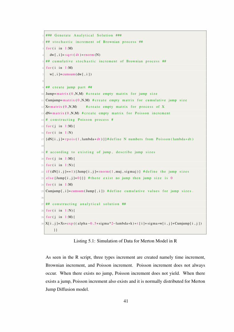
1 ### G e n e r a t e A n a l y t i c a l S o l u t i o n ###

2 ## s t o c h a s t i c i n c r e m e n t o f Brownian p r o c e s s ##

3 f o r ( i i n 1 :M)

4 dw [ , i ]= s q r t ( d t ) * rnorm (N)

5 ## c u m u l a t i v e s t o c h a s t i c i n c r e m e n t o f Brownian p r o c e s s ##

6 f o r ( i i n 1 :M)

7 w[ , i ]= cumsum ( dw [ , i ] )

8

9 ## c r e a t e jump p a r t ##

10 Jump= m a t r i x ( 0 ,N,M) # c r e a t e empty m a t r i x f o r jump s i z e

11 Cumjump= m a t r i x ( 0 ,N,M) # c r e a t e empty m a t r i x f o r c u m u l a t i v e jump s i z e

12 X= m a t r i x ( 0 ,N,M) # c r e a t e empty m a t r i x f o r p r o c e s s o f X

13 dN= m a t r i x ( 0 ,N,M) # c r e a t e empty m a t r i x f o r P o i s s o n i n c r e m e n t

14 # c o n s t r u c t i n g P o i s s o n p r o c e s s #

15 f o r ( j i n 1 :M)

16 f o r ( i i n 1 :N)

17 dN [ i , j ]= r p o i s ( 1 , lambda * d t ) # d e f i n e N numbers from P o i s s o n ( lambda * d t )

18

19 # a c c o r d i n g t o e x i s t i n g o f jump , d e s c r i b e jump s i z e s

20 f o r ( j i n 1 :M)

21 f o r ( i i n 1 :N)

22 i f ( dN [ i , j ]== 1 ) Jump [ i , j ]= rnorm ( 1 , muj , s i g m a j ) # d e f i n e t h e jump s i z e s

23 e l s e Jump [ i , j ]= 0 # t h e r e e x i s t no jump t h e n jump s i z e i s 0

24 f o r ( i i n 1 :M)

25 Cumjump [ , i ]= cumsum ( Jump [ , i ] ) # d e f i n e c u m u l a t i v e v a l u e s f o r jump s i z e s .

26

27 ## c o n s t r u c t i n g a n a l y t i c a l s o l u t i o n ##

28 f o r ( i i n 1 :N)

29 f o r ( j i n 1 :M)

30 X[ i , j ]= Xs* exp ( ( a lpha−0 . 5* sigma ^2−lambda *k ) * t [ i ]+ sigma *w[ i , j ]+ Cumjump [ i , j ] )

Listing 5.1: Simulation of Data for Merton Model in R

As seen in the R script, three types increment are created namely time increment,

Brownian increment, and Poisson increment. Poisson increment does not always

occur. When there exists no jump, Poisson increment does not yield. When there

exists a jump, Poisson increment also exists and it is normally distributed for Merton

Jump Diffusion model.

41

According to the given information, the following simulation paths are yielded. In

Figure 5.1, ten simulated paths are presented. As said before, the simulations are

created for 100 paths but ten paths are only given graphically. The reason is to avoid

complex graphical presentation. As seen in the figure, the paths are nearly exponen-

tially distributed. This pattern is suitable with Levy family. Some paths can be seen

as straight lines. The reason of that these paths take very small values but the others

take higher values. All in all, it can be said that this graphical representation shows

the simulations are exponentially distributed as expected.

0

5

10

15

20

0.00 0.25 0.50 0.75 1.00Time

10Se

lect

edPa

ths

Out

of10

0

Figure 5.1: Simulated Merton Paths

42

5.2 Convergence of Numerical Approximation to Analytical Solution

Generally, it is not possible to obtain the analytical solution of SDEs. At this time,

some numerical approximation methods are used to obtain the solution. As mentioned

in Chapter 2, Milstein method, Runge-Kutta method and Euler-Maruyama method are

well-known numerical approximation methods. Euler-Maruyama method is easy to

compute and it is more suitable for the structure of models which are investigated

in this work. For these reasons, Euler-Maruyama approximation method is used for

numerical approximation procedure. Then, the numerical approximation values are

checked how they converge to the analytical solution. In the simulation process, 100

paths are yielded. Two of them are chosen randomly and their analytical solutions

and numerical solutions are compared in Figure 5.2. In this case, 1000 observations

are used. The time interval is 11000

= 0.001 because dt = TN

where N = 1000 and

T = 1. For numerical approximation method, the following Euler-Maruyama form is

used:

Xtemp = Xs + (α− λk)dtXs + σdWXs, (5.1)

Xapp = Xtemp + (Xtemp(exp(z)− 1)), (5.2)

where Xapp and Xtemp are approximate values for jump case and no-jump case re-

spectively. The parameters α, σ, µj, δ, λ are instantaneous expected return, volatility

of the asset, expected value of jump size, standard deviation of jump size, and jump

intensity, respectively. z is distribution of jump size where z ∼ N(µj, δ2). Xs is

previous state values for approximation chains. To illustrate the convergence perfor-

mance of Euler-Maruyama approximation method, one can check Figure 5.2.

43

0

5

10

0.00 0.25 0.50 0.75 1.00Time

Analytical Solution Euler-Maruyama Approximation

0.00

0.25

0.50

0.75

1.00

1.25

0.00 0.25 0.50 0.75 1.00Time

Analytical Solution Euler-Maruyama Approximation

Figure 5.2: Convergence Between Analytical Solution and Euler Approximation

As seen in Figure 5.2, there exist two graphs. Each one represents one path. Two

paths are chosen out of 100 paths to illustrate graphically. Both paths numerical

approximation perfectly fit to their analytical solutions.

Although the graphical presentation says that the convergence is fine, it is better to

confirm this result by checking convergence performance as time interval changes.

That is, it should be also checked whether all paths with different step sizes have

good convergence or not. For each time interval, average of absolute difference of all

paths for analytical values and numerical approximation values are calculated. Then,

these results are presented in Table 5.1.

44

Time Interval: 20dt 10dt 5dt 2dt dt

Mean of Error Through M Paths: 0.7643 0.4311 0.2698 0.1458 0.0887

Table 5.1: Convergence Rates For Different Time Intervals

As seen in Table 5.1, five time intervals are used for 100 paths. The table shows as

the time interval decreases the convergence between analytical solution and numerical

approximation becomes better. This is the expected result of the convergence process.

5.3 Parameter Estimation of Merton Jump Diffusion Model

In the beginning of the simulation, the initial values are determined for the parame-

ters α, σ, µJ , δ, λ. According to these parameters, the simulation is executed. After

that, we estimate these parameters by using MLE. To do this, number of observations

are taken 1000 and the simulation is repeated 100 times. That is, each parameter is

estimated 100 times and the average of these estimations are taken for each parameter

separately. In Merton model, as a result of having normal distribution of log-return

jump size, the probability density of log-return Yt = ln(XtX0

) can be acquired as fol-

lowing converging form:

P (Yt ∈ A) =∞∑i=0

e−λt(λt)i

i!N(Yt; (α− σ2

2− λk)t+ iµj, σ

2t+ iδ2),

where α, σ, µj , δ, λ are instantaneous expected return, volatility, mean of jump size,

standard deviation of jump size, and jump intensity, respectively. Likelihood function

of this density function is

L(θ;Y ) =T∏t=1

P (Yt). (5.3)

We minimize negative log-likelihood function to make the calculation easier.

− lnL(θ;Y ) = −T∑t=1

lnP (Yt). (5.4)

We have likelihood function. Thus, we are able to construct MLE. This function is

found by using transition density function in the equation 4.26. The following code

is used to obtain parameter estimation and then its output is given in Table 5.2.

45

1 ### MLE of SDE wi th Jump ###

2 dx= m a t r i x ( 0 ,N,M) # c r e a t e empty m a t r i x f o r d i f f e r e n c e o f X s t a t e s

3 f o r ( j i n 1 :M)

4 dx [ , j ]= c ( l o g (X[ 1 , j ] )−l o g ( 1 ) , d i f f ( l o g (X[ , j ] ) ) ) # f i n d d i f f e r e n c e o f X

s t a t e s

5 f = m a t r i x ( 0 ,N, 10 ) # c r e a t e empty m a t r i x f o r t r a n s i t i o n d e n s i t y

6 e s t i m a t e = m a t r i x ( 0 ,M, 5 )

7 f o r ( v i n 1 :M)

8 d i f =dx [ , v ]

9 l i k e l i h o o d = f u n c t i o n ( t h e t a , d i f , d t ) # c r e a t e a f u n c t i o n f o r l i k e l i h o o d

10

11 Q1= t h e t a [ 1 ] # s y m b o l i z e a l p h a p a r a m e t e r

12 Q2= t h e t a [ 2 ] # s y m b o l i z e sigma p a r a m e t e r

13 Q3= t h e t a [ 3 ] # s y m b o l i z e muj p a r a m e t e r

14 Q4= t h e t a [ 4 ] # s y m b o l i z e s i g m a j p a r a m e t e r

15 Q5= t h e t a [ 5 ] # s y m b o l i z e lambda p a r a m e t e r

16 # a s s i g n e l e m e n t o f t r a n s i t i o n d e n s i t y m a t r i x f o r N e l e m e n t s and k jump

p o s s i b i l i t i e s .

17 f o r ( i i n 1 :N)

18 f o r ( j i n 1 : 10 )

19 f [ i , j ] = ( exp(−Q5* d t ) * (Q5* d t ) ^ ( j−1 ) / f a c t o r i a l ( j−1 ) ) * ( 1 / s q r t ( 2* p i * (Q2^2* d t +( j−

1 ) *Q4^2 ) ) ) * exp (−( d i f [ i ] − ( (Q1−Q5*k−Q2^2 / 2 ) * d t +( j−1 ) *Q3 ) ) ^2 / ( 2 * (Q2^2* d t +(

j−1 ) *Q4^2 ) ) )

20 R=rowSums ( f )

21 LL=−sum ( l o g (R) ) # f i n d − l o g l i k e l i h o o d

22 r e t u r n ( LL )

23

24 ## Minimize − l o g l i k e l i h o o d f u n c t i o n ##

25 e s t i m a t i o n = opt im ( c ( 1 , 1 , 1 , 1 , 1 ) , l i k e l i h o o d , g r =NULL, d i f , d t , method="L−BFGS−B" ,

26 l ower =c(− I n f , 0 ,− I n f , 0 ,− I n f ) , uppe r = c ( I n f , I n f , I n f , I n f , I n f ) , h e s s i a n =T )

27 o p t i o n s ( s c i p e n =999 )

28 e s t i m a t e [ v , ] = e s t i m a t i o n \ $ p a r # a s s i g n each p a r a m e t e r e s t i m a t i o n s e t t o

e s t i m a t e m a t r i x .

29

30 p a r a m e t e r _ e s t i m a t i o n s =colSums ( e s t i m a t e ) /M # g i v e t h e e s t i m a t e d p a r a m e t e r

v a l u e f o r each p a r a m e t e r

Listing 5.2: Maximum Likelihood Estimation in R

46

When this algorithm works, the following output is obtained:

α σ µj δ λ

Initial Parameter Values: 2 1.5 0.1 0.3 40

Estimated Parameter Values: 1.7157 1.4972 0.1053 0.2887 38.2364

Table 5.2: Comparison of Initial and Estimated Parameter Values

As seen in Table 5.2, the estimation results are close to initial parameter values. Thus,

this confirms that the parameter estimation process works well. The estimation pro-

cess should be made many times and the averages of these estimations must be taken

to reach the true values because there exists random number generation in the param-

eter estimation algorithm. This random situation causes different estimation results

after the process works. Thus, the parameter estimation gives better and stable results

if the process works many times.

In addition to parameter estimation process, now, we will mention the jump detec-

tion method by using alternative discretization approach which is different from the

method used in this thesis. In the analysis of this thesis, we do not use this method

but we want to give this additional information. This can be helpful for other studies

including scenarios given below.

5.4 Jump Detection in Merton Jump Diffusion Model

Although discretization scheme which is used in this thesis is classical approach, al-

ternative discretization scheme is preferred in some situations. When the jump inten-

sity has bounded and state dependent, this alternative method is used. This method

is based on constructing the jump times by a stochastic time-change of a standard

Poisson process. To illustrate this case, an example is given below. In this example,

a data is simulated and their jump times are determined based on the algorithm given

in Chapter 3. The simulation is created by the following information in Table 5.3.

47

Parameter: α σ µj δ λ dt N T

Value: 3 2 0 1 5 0.01 100 1

Table 5.3: Simulation Initial Values

where α, σ, µj , δ, λ are instantaneous expected return, volatility, mean of jump size,

standard deviation of jump size, and jump intensity, respectively. The number of

observation N = 100 and time is (0 ≤ t ≤ 1) and so T = 1. The time interval dt is

equal to TN

= 1100

= 0.01. Therefore we obtain the Figure 5.3.

0

30

60

90

0.00 0.25 0.50 0.75 1.00Time

Figure 5.3: Simulated Merton Data by Using Discretization Method

48

In the Figure 5.3, there seems to become jumps at six time points, in (0.25, 0.50)

one jump, in (0.50, 0.75) three jumps and in (0.75, 1.00) two jumps. However, this

does not show that they are jump points for this simulation. To confirm that, jump

times are determined by using algorithm in Chapter 3. The result of this algorithm is

represented in Table 5.4.

Jump Times: 0.361 0.367 0.627 0.667

Jump Sizes: 11.207 -7.486 25.841 23.133

Corresponding Values at Jump Points: 13.363 5.877 30.719 42.677

Table 5.4: Jump Sizes, Jump Times and Corresponding Values at Jump Points

As seen in Table 5.4, the jumps become at 0.361, 0.367, 0.627, 0.667 time points.

The corresponding jump values are 13.363, 5.877, 30.719, 42.677. The highest jump

size is seen at time point 0.627. All jumps are upward except at time point 0.367. It

can be said that, there are four jump points in the simulation, although there seems to

be six jump points in the graphic. As a result of being member of Levy family, this

figure shows exponential increasing. Although, the second jump point value is lower

than the other jump values, there exist a increasing as a whole.

49

50

CHAPTER 6

APPLICATON OF MERTON JUMP DIFFISION MODEL ON DOLLAR/TL

EXCHANGE RATE

As mentioned before, the unexpected situations are often seen in many areas such as

economics, biology, chemistry, physics, and social sciences. These situations cause

dramatic changes in value of response. Wars, economic crisis, natural disasters or

similar cases create unexpected effects on models. In financial sector, some sharp

increases and decreases has been seen in market data. The recently seen movements

in exchanges rates of Turkish Lira to foreign currencies are one of the examples for

this case. We worked on the data of daily United States (US) Dollar to Turkish Lira

currency exchange rate. We considered this data has sudden changes and it is suit-

able for Merton Jump Diffusion model. We aim to model this data and to forecast.

In this chapter, Merton Jump Diffusion model and Black-Scholes framework will be

used for modeling the data. For both models , some assumptions required for doing

analysis will be controlled and then the analysis will be made. Firstly, the param-

eter estimations will be applied. Then, AIC will be used to determine the better fit

to empirical data. Moreover, MAPE for both two models are calculated to see the

forecasting accuracy performance of them.

6.1 Dollar/TL Exchange Rate Data and Jump Detection

In the analysis, the used data, which is daily US Dollar to Turkish Lira exchange rate,

is taken between the date of 01.02.2019 and 21.06.2019. In this interval, there are

121 data points. The data is given in the Figure 6.1. As seen in the figure, the data

includes some sudden increasing/decreasing. It has an overall increasing trend.

51

5.25

5.50

5.75

6.00

Feb 2019 Mar 2019 Apr 2019 May 2019 Jun 2019Time

Figure 6.1: Dollar to Turkish Lira Exchange Rate

The log-return of data is taken to determine jump points and the Figure 6.2 is created

. We define the (−0.0125, 0.0125) as cut-off points for log-return exchange rate data.

As seen in this figure, these points are determined by red line. The points which

are out of these lines are accepted jump points. According to the Figure 6.2 and the

calculations based on given threshold, there exist 9 jump points.

-0.025

0.000

0.025

0.050

0.00 0.25 0.50 0.75 1.00Time

Log

Ret

urns

Figure 6.2: Log-Return Exchange Rate For Detecting Jump Points

52

6.2 Assessing The Model Assumptions

Model assumptions are requirement for testing the data. Before applying parameter

estimation, we should mention model assumptions and their checking. As said be-

fore, Merton Jump Diffusion model includes Brownian motion and Poisson process,

Black-Scholes model includes Brownian motion. These processes must satisfy three

conditions namely stationarity, normality and independence. Thus, we check three

assumptions according to the following log-return model:

ln(Xt

Xt−1

) = (α− σ2

2− λk)dt+ σWt +

Nt∑i=1

Qi (6.1)

6.2.1 Stationarity

Stationary time series causes constant sample statistics such as mean, variance and

autocorrelation in time. Many forecasting methods need the stationarity assumption

to obtain accurate prediction. Otherwise, unexpected acts in the analysis can be seen.

For example, a test statistics, t, is not following t-distribution. The mean or variance

can be increased with sample size if the time series persistently increases in time. This

causes to undervalue the mean and variance in coming periods. In this application,

stationarity is checked for Merton and Black-Scholes model according to log-return

ln( XtXt−1

). In the analysis, we use two tests namely KPSS test and ADF test to check

stationarity.

• Hypothesis Test for KPSS Test:

H0: Distribution is stationary.

H1: Distribution is not stationary.

• Hypothesis Test for ADF Test:

H0: Distribution is not stationary.

H1: Distribution is stationary.

If the null hypothesis is rejected in KPSS test, then time series does not have unit root

or it is not stationary. If the null hypothesis is rejected in ADF test, then time series

is stationary.

53

6.2.2 Normality

Normality are checked for Merton model according to the following form which is

distributed standard normal N(0,1).

ln( XtXt−1

)−∑Nt

i=1Qi − µtσ√t

(6.2)

where µ and σ are mean and standard deviation of jump size distribution. Black-

Scholes model normality assumpiton is controlled for ln( XtXt−1

). Although the easiest

way of detecting normality is graphical presentation. This is not accurate so we prefer

to use statistical test Shapiro-Wilk and Jarque-Bera test. The hypothesis for normality

is:

• Hypothesis Test for Shapiro-Wilk or Jarque-Bera Test:

H0: Distribution is normally distributed.

H1: Distribution is not normally distributed.

If the null hypothesis is rejected, then the normality assumption is satisfied.

6.2.3 Independence

Box-Ljung or Box-Pierce test can be used as statistical test to obtain exact result

of independence checking. With this test, we can see whether the increments are

independent or not. Independence are checked for both model according to the log-

return ln( XtXt−1

).

• Hypothesis Test for Box-Pierce Test:

H0: Distribution is independently distributed.

H1: Distribution is not independently distributed.

If the null hypothesis does not rejected, then the independent increment assumption

is satisfied.

Now, let us check the these three assumption whether they are satisfied or not. To

do this, we will construct some test statistics mentioned above. The results are in

Table 6.1:

54

Merton Jump Diffusion Model Black-Scholes Model

Stationarity Normality Independence Stationarity Normality Independence

KPSS 0.10 - - 0.10 - -

ADF 0.01 - - 0.01 - -

Shapiro-Wilk - 0.06 - - ≈0 -

Jarque-Bera - 0.75 - - ≈0 -

Box-Pierce - - 0.35 - - 0.35

Table 6.1: P-Values of Some Test Statistics for Model Assumption Checkings

As seen in Table 6.1, stationarity assumption is satisfied for both Merton Jump Dif-

fusion model and Black-Scholes model because p-value for KPSS test is bigger than

critical value 0.05 and p-value for ADF test is less than 0.05. This indicates there

is no enough evidence to reject the increments are stationary. In the normality as-

sumption for Merton Jump Diffusion model, Shapiro-Wilk and Jarque-Bera tests say

that p values are bigger than critical values. That is, the null hypothesis which is

increments are normally distributed is not rejected. Thus, normality assumption is

satisfied. However, this assumption is not satisfied for Black-Scholes model due to

the very small p-values. The last assumption which is independence for both models

is satisfied. Box-Pierce test confirms this result with the p-values which are bigger

than critical value 0.05. Moreover, Merton Jump Diffusion model has two additional

assumptions. The distribution of logarithm of jump size is normal and interarrival

times of jump point is exponentially distributed. The normality is checked for the

following form:ln(∆j)− µ

σ

Here, ∆j is jth jump size where j is the number of jump. µ, σ are mean and standard

deviation of jump sizes respectively. We check the standard normality based on this

form. According to the Shapiro-Wilk test p-value for normality is 0.22. This indicates

the logarithm of jump size distribution is standard normal. Since, the p-value is less

the critical value 0.05. The other assumption which is exponential distributed jump

arrival times is controlled by using Kolmogorov-Smirnov test. In this test, the null

hypothesis is the interarrival times of jumps is distributed exponential. The p-value

obtained from this test is 0.18, that is, the null hypothesis is not rejected. Since, p-

55

value is less than the critical value 0.05. Therefore, we can say the jump arrival times

is exponentially distributed.

6.3 Parameter Estimation of Merton Jump Diffusion Model For USD/TL Ex-

change Rate

The following Merton Jump Diffusion model is given by the equation 4.19.

dXt = (α− λk)Xtdt+ σXtdWt + (yt − 1)XtdNt

Here Wt and Nt are Brownian motion and Poisson process, respectively. The symbol

of λ is intensity of Poisson process, α is instantaneous expected return, σ is diffusion

term, yt − 1 is relative jump size, and its mean is k. In Merton model, as a result

of having normal distribution of log-return jump size, the probability density of log-

return Yt = ln(XtX0

) can be acquired as the following converging form:

P (Yt ∈ A) =∞∑i=0

e−λt(λt)i

i!N(Yt; (α− σ2

2− λk)t+ iµj, σ

2t+ iδ2),

where α, σ, µj , δ, λ are instantaneous expected return, volatility, mean of jump size,

standard deviation of jump size, and jump intensity, respectively. Likelihood function

of this transition density function is given by the equation 5.3.

L(θ;Y ) =T∏t=1

P (Yt).

After the process of MLE estimation is completed, the following results come out:

α σ µj δ λ

Estimated Parameter Values: 0.238 0.063 -0.015 0.058 4.440

Table 6.2: Merton Jump Diffusion Model Parameter Estimations For Exchange Rate

As seen in Table 6.2, we find the five parameters values for Merton Diffusion model

after the process of parameter estimation. According to this, the expected return and

volatility are 0.238 and 0.063 respectively. The jump size distribution’s expected

56

value and standard deviation are −0.015 and 0.058, respectively. The jump intensity

is 4.44. In other words , we expect 4 jumps in the US Dollar to Turkish Lira currency

exchange rate data between the date of 01.02.2019 and 23.06.2019 averagely.

6.4 Parameter Estimation of Black Scholes Model For USD/TL Exchange Rate

The parameters of daily US Dollar to Turkish Lira currency exchange rate data will

also be estimated by using Black-Scholes framework. To do this, the following Black-

Scholes model is used:

dt = µXtdt+ σXtdWt, (6.3)

where µ is drift parameter and σ is diffusion parameter. The transition density func-

tion is

P (Yt) =1√

2πσ2exp

(− (dXt − µXtdt)

2

2σ2Xtdt

), (6.4)

where dXt = Xt −Xt−1 and dt = tn − tn−1

After the process of MLE estimation is completed, the following results come out:

µ σ

Estimated Parameter Values: 0.112 0.114

Table 6.3: Black-Scholes Model Parameter Estimations For Exchange Rate

As seen in Table 6.3, the drift parameter µ takes the value of 0.112 and diffusion

parameter σ takes the value of 0.114.

6.5 Comparison of Merton Jump Diffusion Model and Black Scholes Model

For USD/TL Exchange Rate

The daily US Dollar to Turkish Lira exchange rate data was modelled considering

both two structure of Black-Scholes and Merton Jump Diffusion. To determine which

57

model has better fit to this data, AIC is used for both models. AIC is calculated as

follows:

AIC = −2 lnL+ 2k (6.5)

where L is the value of likelihood function, N is the number of observations, and k is

the number of parameters. The best model is the one that has minimum AIC among

the other models. The following results are found when the AIC calculated for two

models:

Merton Model Black-Scholes Model

AIC: 352.04 356.61

Table 6.4: AIC For Merton and Black-Scholes Models

The better model in the comparison has the smallest AIC value. Thus, Merton Jump

Diffusion model is better model than Black-Scholes model for daily US Dollar to

Turkish Lira exchange rate data according to Table 6.4.

6.6 Prediction on US Dollar to Turkish Lira Exchange Rate

We made parameter estimation for Black-Scholes and Merton Jump Diffusion model

by using MLE for USD/TL exchange rate data between date of 01.02.2019 and 21.06.2019.

In this interval, there are 121 data points. Now, we make prediction for the exchange

rate between date of 23.06.2019 and 02.07.2019. To do this, we used these two models

with estimated parameter values. Moreover, MAPE is used to measure how accurate

the forecasting results. It is calculated for two models according to the following

structure:

MAPE =( 1

n

∑ |Actual − Forecasting||Actual|

)100, (6.6)

where n is number of observations. If the results are less than 10 we can consider the

model forecasting accuracy performance is good.

58

In the following table, the prediction values which are found for between the date

of 23.06.2019 and 02.07.2019 are presented. As seen in the table, the prediction

values of Merton model is more close to actual values in all days. However, Black-

Scholes predictions have more deviation from the actual data set. After the fifth day,

Black-Scholes model very largely deviate from the actual values. Also, the predic-

tion MAPE values are calculated for both model to determine which model has better

forecasting accuracy. According to the results in Table 6.5, Merton Jump Diffusion

model prediction values are closer to the actual values. Merton jump Diffusion model

has smaller MAPE value which is 2.91% and Black-Scholes model has 4.71% MAPE

value. It can be said that Merton Jump Diffusion model has better forecasting accu-

racy performance than Black-Scholes model for this data set.

Date True Value Merton Prediction Black-Scholes Prediction

23.06.2019 5.76 5.84 5.92

24.06.2019 5.81 5.87 5.91

25.06.2019 5.80 5.86 5.91

26.06.2019 5.78 5.89 5.97

27.06.2019 5.77 5.86 5.99

28.06.2019 5.79 5.92 6.17

30.06.2019 5.74 5.98 6.14

01.07.2019 5.65 5.99 6.08

02.07.2019 5.65 6.02 6.08

MAPE: 2.91 4.71

Table 6.5: Merton and Black-Scholes Model Forecasting Performance

59

From the Figure 6.2, we can see that Merton model has almost same path with actual

values up to fifth day. After this point, both model prediction values deviate from

actual values but this deviation is higher for Black-Scholes model. Also, we can see

from the figure Merton model has closer values at all points to actual values than

Black-Scholes model.

5.7

5.8

5.9

6.0

6.1

Jun 24 Jun 26 Jun 28 Jun 30 Jul 02Time

Actual Values Black-Scholes Prediction Merton Prediction

Figure 6.3: Comparison of Actual Values, Merton Jump Diffusion Model and Black-

Scholes Model Predictions

60

CHAPTER 7

CONCLUSION

In many branches, measuring the rate of change has become more and more important

over the years. This situation has made the differential equation more widely used.

Moreover, stochastic movement in differential equations and so SDE are frequently

used for many purposes. By using SDE, it is possible to have information about

randomness or uncertainty in the models. In the thesis, we mainly focus on SDE with

jump models. These models have ability to measure the radical changes in quantities

due to some reasons such as wars, natural disasters, market crashes or some dramatic

news as well as moderate changes.

In this work, we have two purposes. First one is to estimate parameter values in

Merton Jump Diffusion models. In Chapter 5, the data was simulated according to

Merton Jump Diffusion model. We found that the initial parameter values used for the

simulating data and parameter estimation values by using MLE are very close to each

other as seen in the Table 5.3. To obtain parameter values truly, the estimation process

was made many times due to including random number generation from Normal and

Poisson distribution. After that, the average of these estimation process was taken.

As iteration number of estimation process increases, the estimation results are closer

to initial parameter values. The reason of this situation is eliminating the potential

bias yielded by random number generator [9]. In Chapter 5, we also checked whether

numerical approximation and analytical solution values are close to each other or not.

As seen in Figure 5.2, the convergence seems to be perfect. Euler-Maruyama method

was used for numerical approximation. As mentioned earlier, most of the times an-

alytical solutions are difficult to obtain or sometimes not even obtained. For this

kind of situations, these numerical solution values can be used instead of analytical

61

solution. Therefore, it is important that the algorithm, which we adapted to obtain nu-

merical approximation, works well. Moreover, we adapted jump detection algorithm

in Chapter 3 to determine jump times and jump sizes. However, this algorithm was

not used in our analysis because this jump detection algorithm is used for unbounded

jump intensity. In Merton model, jump intensity is constant and so the classical dis-

cretization scheme was used. We mentioned this discretization algorithm to become

reference for other studies including Jump Diffusion models with unbounded jump

intensity.

The second purpose of this study is to show Merton model has better fit to US Dollar

to Turkish Lira exchange rate data than Black-Scholes counterpart. The US Dollar to

Turkish Lira exchange rate data has showed sudden increase/decrease in recent years.

Therefore, it includes many jumps especially upward jumps. We considered jump dif-

fusion models can be compatible with the trend of this data and it has better fit to this

data than the other diffusion models. Among various jump diffusion models we have

preferred trying the Merton Jump Diffusion model since the data set satisfies its as-

sumptions. Once, the Merton model was fitted for the data the parameter estimations

were conducted both for the Merton Jump Diffusion model and the Black-Scholes

model. Then, these two models were compared in terms of forecast performance and

model fit. Firstly, we checked the AIC values for both models in Chapter 6 to con-

trol model fit performances. Merton Jump Diffusion model has better fit to the data

because AIC values for Merton model is lower than AIC for Black-Scholes model as

seen in Table 6.4. This result was found as expected because the exchange rate data

includes many jumps and we know that Black-Scholes model is insensitive to this

jumps. Secondly, we made 9 days prediction by using the exchange rate data with

Merton and Black-Scholes model. The predictions were controlled with MAPE val-

ues for both models. As expected, Merton Jump Diffusion model has smaller MAPE

value. Thus, the predictions of Merton Jump Diffusion model is more close to original

values. Also, we present the forecasting trends for these two models with actual data

set graphically. This also confirms that Merton prediction is more close to actual data

for all days. Therefore, Merton Jump Diffusion model has better forecasting accuracy

performance than Black-Scholes model for US Dollar to Turkish Lira exchange rate

data.

62

Both Merton model and Black-Scholes model have some assumptions to study on

them. Before doing analysis, we must check the all assumptions. In Chapter 6, we

investigated three assumptions for both models namely stationarity, normality and in-

dependence of increments. Also, we checked two additional assumptions for Merton

Jump Diffusion model. First one is that the logarithm of jump sizes is distributed

normal. Second one is that interarrival times of jumps is distributed exponential. The

stationarity assumption is satisfied for both models. That is, the probability of any

increments does not depend location of time interval. They only depend on length

of time intervals. Stationarity prevents the unreliable and spurious outputs obtained

in the analysis. These outputs can cause weak understanding and forecasting. How-

ever, the normality assumption is only satisfied for Merton model. Non-normality

obstructs exact inference on estimations of coefficients. This assumption is not sat-

isfied for Black-Scholes model and this result is expected. Since, the data includes

some jump points and this made the distribution of ln( XtXt−1

)become non-normal. This

is also answer the why this data is more suitable with Merton Jump Diffusion model.

The last assumption independent increments is satisfied for both models. The Merton

additional assumptions which are normally distributed logarithm of jump size and

exponentially distributed interarrival times of jumps are also satisfied.

In conclusion, Merton Jump Diffusion model is a better fit than the Black-Schooles

model for US Dollar to Turkish Lira exchange rate data set since it captures the jump

points as well as the continuous parts. The Black-Scholes framework is insensitive

to jumps in the data set. The US Dollar to Turkish Lira exchange rate data has both

discrete and continuous parts. Thus, Merton Jump Diffusion model explains the data

better.

63

64

REFERENCES

[1] ALLEN, E. Modeling with Itô Stochastic Differential Equations, vol. 22.

Springer Netherlands, 2007.

[2] BASS, R. F. Stochastic differential equations with jumps. Probab. Surveys 1

(2004), 1–19.

[3] BHATTACHARYA, R., AND WAYMIRE, E. Stochastic Processes with Appli-

cations. Classics in Applied Mathematics. Society for Industrial and Applied

Mathematics, 2009.

[4] BOYCE, W., AND DIPRIMA, R. Elementary Differential Equations and Bound-

ary Value Problems, 10th Edition. Wiley, 2012.

[5] CARLSSON, J., MOON, K.-S., SZEPESSY, A., TEMPONE, R., AND

ZOURARIS, G. Stochastic Differential Equations: Models and Numerics 1.

KTH, 2019.

[6] DITLEVSEN, S., AND SAMSON, A. Introduction to stochastic models in biol-

ogy. Lecture Notes in Mathematics 2058 (01 2010).

[7] GEISS, S. Lecture notes: Stochastic differential equations. =

http://users.jyu.fi/ geiss/lectures/stochasticsde.pdf, March 2018.

[8] GIESECKE, K., AND TENG, G. Numerical solution of jump-diffusion sdes.

Tech. rep., Stanford University, 2013.

[9] GONZÁLEZ-URTEAGA, A., NOVALES, A., AND RUBIO, G. Estimation of

stochastic volatility models with jumps in returns for stock market indices.

Tech. rep., Universidad del País Vasco, 2019.

[10] HANSON, F. B. Applied Stochastic Processes and Control for Jump-Diffusions:

Modeling, Analysis, and Computation (Advances in Design and Control).

SIAM.

65

[11] HANSON, F. B., AND WESTMAN, J. J. Stochastic analysis of jump-diffusions

for financial log-return processes. In Stochastic Theory and Control (Berlin,

Heidelberg, 2002), B. Pasik-Duncan, Ed., Springer Berlin Heidelberg, pp. 169–

183.

[12] HAUGH, M. A brief introduction to stochastic calculus. Tech. rep., Columbia

University, 2016.

[13] IBE, O. Markov Processes for Stochastic Modeling. Stochastic modeling. El-

sevier Science, 2008.

[14] MATSUDA, K. Introduction to merton jump diffusion model. Tech. rep., The

City University of New York, 2004.

[15] MERTON, R. C. Option pricing when underlying stock returns are discontinu-

ous. Journal of Financial Economics 3, 1-2 (1976), 125–144.

[16] MIKOSCH, T. Elementary Stochastic Calculus with Finance in View. Advanced

series on statistical science & applied probability. World Scientific, 1998.

[17] PRIVAULT, N. Lecture notes: Stochastic calculus for jump pro-

cesses. = http://www.ntu.edu.sg/home/nprivault/MA5182/stochastic-calculus-

jump-processes.pdf.

[18] REDUCHA, W. Parameter estimation of the pareto-beta jump-diffusion model

in times of catastrophe crisis. Tech. rep., Halmstad University, Applied Mathe-

matics and Physics (CAMP), 2011.

[19] ROSS, S. Differential Equations. Wiley, 1984.

[20] SAUER, T. Numerical solution of stochastic differential equations in finance.

In Handbook of Computational Finance, J.-C. Duan, W. K. Hardle, and J. E.

Gentle, Eds. Springer, Berlin-Heidelberg, 2012, ch. 19, pp. 529–550.

[21] SERFOZO, R. Basics of Applied Stochastic Processes. Probability and Its Ap-

plications. Springer Berlin Heidelberg, 2009.

[22] SIGMAN, K. Lecture notes: Geometric brownian motion, modeling stock prices

in continuous time, black-scholes option pricing formula. http://www.

66

columbia.edu/~ks20/FE-Notes/4700-07-Notes-GBM.pdf,

2006.

[23] TANKOV, P. Financial Modelling with Jump Processes. Chapman and Hal-

l/CRC Financial Mathematics Series. CRC Press, 2003.

[24] WHITT, W. A quick introduction to stochastic calculus. =

http://www.columbia.edu/ ww2040/4701Sum07/lec0813.pdf.

[25] WIKIPEDIA. Markov property, 2019. [Online; last edited 3-July-2019].

[26] WINKEL, B. Shen, wen. 2015. lecture notes for math 251:

Introduction to ordinary and partial differential equations. =

https://www.simiode.org/resources/2947, Oct 2016.

67

68

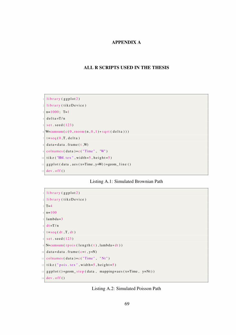
APPENDIX A

ALL R SCRIPTS USED IN THE THESIS

1 l i b r a r y ( g g p l o t 2 )

2 l i b r a r y ( t i k z D e v i c e )

3 n=1000 ; T=1

4 d e l t a =T / n

5 s e t . s eed ( 123 )

6 W=cumsum ( c ( 0 , rnorm ( n , 0 , 1 ) * s q r t ( d e l t a ) ) )

7 t = seq ( 0 ,T , d e l t a )

8 d a t a = d a t a . f rame ( t ,W)

9 co lnames ( d a t a ) =c ( " Time " , "W" )

10 t i k z ( "BM. t e x " , wid th =5 , h e i g h t =5 )

11 g g p l o t ( da t a , a e s ( x=Time , y=W) ) +geom_ l i n e ( )

12 dev . o f f ( )

Listing A.1: Simulated Brownian Path

1 l i b r a r y ( g g p l o t 2 )

2 l i b r a r y ( t i k z D e v i c e )

3 T=4

4 n=100

5 lambda=3

6 d t =T / n

7 t = seq ( dt , T , d t )

8 s e t . s eed ( 123 )

9 N=cumsum ( r p o i s ( l e n g t h ( t ) , lambda * d t ) )

10 d a t a = d a t a . f rame ( c= t , y=N)

11 co lnames ( d a t a ) =c ( " Time " , " Nt " )

12 t i k z ( " p o i s . t e x " , wid th =5 , h e i g h t =5 )

13 g g p l o t ( ) +geom_ s t e p ( da t a , mapping= a e s ( x=Time , y=Nt ) )

14 dev . o f f ( )

Listing A.2: Simulated Poisson Path

69

1 ### G e n e r a t e A n a l y t i c a l S o l u t i o n ###

2 s e t . s eed ( 127 ) # c r e a t e r e p r o d u c i b l e r e s u l t s

3 ## d e f i n e t h e i n i t i a l p a r a m e t e r v a l u e s f o r p r o c e s s ##

4 a l p h a =2 # i n s t a n t a n e o u s e x p e c t e d r e t u r n

5 s igma=1 . 5 # v o l a t i l i t y o f a s s e t

6 muj=0 . 1 # e x p e c t e d v a l u e f o r d i s t r i b u t i o n o f jump s i z e

7 s i g m a j =0 . 3 # s t a n d a r d d e v i a t i o n f o r d i s t r i b u t i o n o f jump s i z e

8 lambda=40 # jump i n t e n s i t y

9 k=exp ( muj+0 . 5* s i g m a j ^2 )−1 #mean of r e l a t i v e jump s i z e

10 M=100 # number o f p a t h s

11 Xs=1 # s t a r t i n g v a l u e f o r p r o c e s s o f X

12 N=1000 # number o f o b s e r v a t i o n s

13 T=1 # l e n g t h o f t h e i n t e r v a l and t ime i s i n [ 0 , T ]

14 d t =T /N # t ime i n c r e m e n t

15 t = seq ( dt , 1 , d t ) # t ime i n c r e a s e by d t .

16 dw= m a t r i x ( 0 ,N,M) # c r e a t e empty m a t r i x f o r dw

17 w= m a t r i x ( 0 ,N,M) # c r e a t e empty m a t r i x f o r w

18

19 ## s t o c h a s t i c i n c r e m e n t o f Brownian p r o c e s s ##

20 f o r ( i i n 1 :M)

21 dw [ , i ]= s q r t ( d t ) * rnorm (N)

22 ## c u m u l a t i v e s t o c h a s t i c i n c r e m e n t o f Brownian p r o c e s s ##

23 f o r ( i i n 1 :M)

24 w[ , i ]= cumsum ( dw [ , i ] )

25 ## c r e a t e jump p a r t ##

26 Jump= m a t r i x ( 0 ,N,M) # c r e a t e empty m a t r i x f o r jump s i z e

27 Cumjump= m a t r i x ( 0 ,N,M) # c r e a t e empty m a t r i x f o r c u m u l a t i v e jump s i z e

28 X= m a t r i x ( 0 ,N,M) # c r e a t e empty m a t r i x f o r p r o c e s s o f X

29 dN= m a t r i x ( 0 ,N,M) # c r e a t e empty m a t r i x f o r P o i s s o n i n c r e m e n t

30 # c o n s t r u c t i n g P o i s s o n p r o c e s s #

31 f o r ( j i n 1 :M)

32 f o r ( i i n 1 :N)

33 dN [ i , j ]= r p o i s ( 1 , lambda * d t ) # d e f i n e N numbers from P o i s s o n ( lambda * d t )

34 # a c c o r d i n g t o e x i s t i n g o f jump , d e s c r i b e jump s i z e s

35 f o r ( j i n 1 :M)

36 f o r ( i i n 1 :N)

37 i f ( dN [ i , j ]== 1 ) Jump [ i , j ]= rnorm ( 1 , muj , s i g m a j ) # d e f i n e t h e jump s i z e s

38 e l s e

39 Jump [ i , j ]= 0 # t h e r e e x i s t no jump t h e n jump s i z e i s 0

40 f o r ( i i n 1 :M)

70

41 Cumjump [ , i ]= cumsum ( Jump [ , i ] ) # d e f i n e c u m u l a t i v e v a l u e s f o r jump s i z e s .

42

43 ## c o n s t r u c t i n g a n a l y t i c a l s o l u t i o n ##

44 f o r ( i i n 1 :N)

45 f o r ( j i n 1 :M)

46 X[ i , j ]= Xs* exp ( ( a lpha−0 . 5* sigma ^2−lambda *k ) * t [ i ]+ sigma *w[ i , j ]+ Cumjump [ i , j ] )

47 # ##################################

48 ## produce t h e graph of Merton s i m u l a t i o n s ##

49 l i b r a r y ( g g p l o t 2 )

50 l i b r a r y ( t i k z D e v i c e )

51 t = seq ( dt , T , d t )

52 d a t a = d a t a . f rame ( t ,X)

53 t i k z ( " Merton _ S i m u l a t i o n s . t e x " , wid th =5 , h e i g h t =5 )

54 f 1=geom_ l i n e ( a e s ( x= t , y=X[ , 10 ] , c o l o r = " b l a c k " ) )

55 f 2=geom_ l i n e ( a e s ( x= t , y=X[ , 20 ] , c o l o r = " r e d " ) )

56 f 3=geom_ l i n e ( a e s ( x= t , y=X[ , 30 ] , c o l o r = " b l u e " ) )

57 f 4=geom_ l i n e ( a e s ( x= t , y=X[ , 40 ] , c o l o r = " maroon " ) )

58 f 5=geom_ l i n e ( a e s ( x= t , y=X[ , 50 ] , c o l o r = " g r e e n " ) )

59 f 6=geom_ l i n e ( a e s ( x= t , y=X[ , 60 ] , c o l o r = " brown " ) )

60 f 7=geom_ l i n e ( a e s ( x= t , y=X[ , 70 ] , c o l o r = " p ink " ) )

61 f 8=geom_ l i n e ( a e s ( x= t , y=X[ , 80 ] , c o l o r = " magenta " ) )

62 f 9=geom_ l i n e ( a e s ( x= t , y=X[ , 90 ] , c o l o r = " cyan " ) )

63 f 10=geom_ l i n e ( a e s ( x= t , y=X[ , 100 ] , c o l o r = " pe ru " ) )

64 g g p l o t ( d a t a ) + f 1+ f 2+ f 3+ f 4+ f 5+ f 6+ f 7+ f 8+ f 9+ f 10+ x l a b ( " Time " ) + y l a b ( " 10 S e l e c t e d

P a t h s Out o f 100 " ) + theme ( l e g e n d . p o s i t i o n = " none " )

65 dev . o f f ( )

66 # #################################

67 ## Numer ica l Approx ima t ion by Using Eule r−Maruyama Method ##

68 X_ app= m a t r i x ( 0 ,N,M) # c r e a t e empty m a t r i x f o r a p p r o x i m a t i o n v a l u e s f o r

p r o c e s s o f X

69 Xs=1

70 f o r ( j i n 1 :M)

71 f o r ( i i n 1 :N)

72 xapptemp=Xs+ d t * ( a lpha−lambda *k ) *Xs+sigma *Xs*dw [ i , j ]

73 X_ app [ i , j ]= xapptemp +( xapptemp *( exp ( Jump [ i , j ] )−1 ) ) *dN [ i , j ]

74 Xs=X_ app [ i , j ]

75 Xs=1

76

77 #show t h e c o n v e r g e n c e o f a n a l y t i c a l s o l u t i o n and Eule r−Maruyama

71

a p p r o x i m a t i o n s #

78 i n s t a l l . p a c k a g e s ( " g g p l o t 2 " )

79 i n s t a l l . p a c k a g e s ( " t i k z D e v i c e " )

80 l i b r a r y ( g g p l o t 2 )

81 l i b r a r y ( t i k z D e v i c e )

82 d a t a 1= d a t a . f rame ( t ,X[ , 25 ] )

83 co lnames ( d a t a 1 ) =c ( " t ime " , " v a l u e " )

84 d a t a 2= d a t a . f rame ( t ,X_ app [ , 25 ] )

85 co lnames ( d a t a 2 ) =c ( " t ime " , " v a l u e " )

86 p= g g p l o t ( ) +geom_ l i n e ( d a t a = d a t a 1 , a e s ( x= t ime , y=X[ , 25 ] , c o l o r =" A n a l y t i c a l

S o l u t i o n " ) ) +geom_ l i n e ( d a t a = d a t a 2 , a e s ( x= t ime , y=X_ app [ , 25 ] , c o l o r =" Eu le r−

Maruyama Approx ima t ion " ) ) + x l a b ( " Time " ) + y l a b ( " " ) + theme ( l e g e n d . p o s i t i o n

=" bot tom " ) + s c a l e _ c o l o r _ manual ( v a l u e s =c ( " b l a c k " , " r e d " ) ) + theme ( l e g e n d .

t i t l e = e l e m e n t _ b l a n k ( ) )

87 p1=p + theme ( l e g e n d . t e x t = e l e m e n t _ t e x t ( margin = margin ( r =15 , l = 5 , u n i t =

" p t " ) , h j u s t = 0 ) )

88 d a t a 3= d a t a . f rame ( t ,X[ , 75 ] )

89 co lnames ( d a t a 3 ) =c ( " t ime " , " v a l u e " )

90 d a t a 4= d a t a . f rame ( t ,X_ app [ , 75 ] )

91 co lnames ( d a t a 4 ) =c ( " t ime " , " v a l u e " )

92 p= g g p l o t ( ) +geom_ l i n e ( d a t a = d a t a 3 , a e s ( x= t ime , y=X[ , 75 ] , c o l o r =" A n a l y t i c a l

S o l u t i o n " ) ) +geom_ l i n e ( d a t a = d a t a 4 , a e s ( x= t ime , y=X_ app [ , 75 ] , c o l o r =" Eu le r−

Maruyama Approx ima t ion " ) ) + x l a b ( " Time " ) + y l a b ( " " ) + theme ( l e g e n d . p o s i t i o n

=" bot tom " ) + s c a l e _ c o l o r _ manual ( v a l u e s =c ( " b l a c k " , " r e d " ) ) + theme ( l e g e n d .

t i t l e = e l e m e n t _ b l a n k ( ) )

93 p2=p + theme ( l e g e n d . t e x t = e l e m e n t _ t e x t ( margin = margin ( r = 15 , l =5 , u n i t =

" p t " ) , h j u s t = 0 ) )

94 # t o combine two g r a p h s i n one pane l , use f o l l o w i n g p a c k a g e s

95 i n s t a l l . p a c k a g e s ( " g r i d E x t r a " )

96 l i b r a r y ( g r i d E x t r a )

97 t i k z ( " c o n v e r g e n c e . t e x " , wid th =5 , h e i g h t =5 )

98 g r i d . a r r a n g e ( p1 , p2 , nrow=2 )

99 dev . o f f ( )

100 # ################################

101 ## E u l e r c o n v e r g e n c e check ##

102 Xs=1 # i n i t i a l v a l u e

103 d e l t a =5 # number o f d i f f e r e n t t ime i n t e r v a l ( d t ) s i z e s

104 Xerr = m a t r i x ( 0 ,M, d e l t a ) # c r e a t e empty m a t r i x f o r e r r o r

105 # A n a l y t i c a l s o l u t i o n

106 f o r ( j i n 1 :M)

72

107 Xs=1

108 Xtrue =Xs* exp ( ( a lpha−0 . 5* sigma ^2−lambda *k ) * t [N]+ sigma *w[N, j ]+ Cumjump [N, j ] )

109 R=c ( 1 , 2 , 5 , 10 , 20 ) # m u l t i p l i e r o f d t

110 f o r ( p i n 1 : 5 )

111 Dt=R[ p ]* d t # t ime i n t e r v a l f o r e u l e r a p p r o x i m a t i o n

112 L=N/ R[ p ] # number o f o b s e r v a t i o n s f o r e u l e r a p p r o x i m a t i o n

113 Xs=1

114 f o r ( i i n 1 : L )

115 Winc=sum ( dw [ ( R[ p ] * ( i−1 ) +1 ) : ( R[ p ]* i ) , j ] ) # Brownian i n c r e m e n t f o r e u l e r

a p p r o x i m a t i o n

116 Ninc=sum ( Jump [ ( R[ p ] * ( i−1 ) +1 ) : ( R[ p ]* i ) , j ] ) # P o i s s o n i n c r e m e n t f o r e u l e r

a p p r o x i m a t i o n

117 x t e m p e r r =Xs+Dt * ( a lpha−lambda *k ) *Xs+sigma *Xs*Winc

118 X_em= x t e m p e r r +( x t e m p e r r * ( exp ( Ninc )−1 ) ) # E u l e r a p p r o x i m a t i o n

119 Xs=X_em

120 Xerr [ j , p ]= abs (X_em−Xtrue ) # a s s i g n each d i f f e r e n c e between a n a l y t i c a l and

a p p r o x i m a t i o n r e s u l t t o t h i s m a t r i x

121 # P r e s e n t t h e r e s u l t o f mean of e r r o r t h r o u g h t h e M p a t h s

122 colSums ( Xerr ) / 100

123 # ##############################

124 ### MLE of SDE wi th Jump ###

125 dx= m a t r i x ( 0 ,N,M) # c r e a t e empty m a t r i x f o r d i f f e r e n c e o f X s t a t e s

126 f o r ( j i n 1 :M)

127 dx [ , j ]= c ( l o g (X[ 1 , j ] )−l o g ( 1 ) , d i f f ( l o g (X[ , j ] ) ) ) # f i n d d i f f e r e n c e o f X s t a t e s

128 f = m a t r i x ( 0 ,N, 10 ) # c r e a t e empty m a t r i x f o r t r a n s i t i o n d e n s i t y

129 e s t i m a t e = m a t r i x ( 0 ,M, 5 )

130 f o r ( v i n 1 :M)

131 d i f =dx [ , v ]

132 l i k e l i h o o d = f u n c t i o n ( t h e t a , d i f , d t ) # c r e a t e a f u n c t i o n f o r l i k e l i h o o d

133 Q1= t h e t a [ 1 ] # s y m b o l i z e a l p h a p a r a m e t e r

134 Q2= t h e t a [ 2 ] # s y m b o l i z e sigma p a r a m e t e r

135 Q3= t h e t a [ 3 ] # s y m b o l i z e muj p a r a m e t e r

136 Q4= t h e t a [ 4 ] # s y m b o l i z e s i g m a j p a r a m e t e r

137 Q5= t h e t a [ 5 ] # s y m b o l i z e lambda p a r a m e t e r

138 # a s s i g n e l e m e n t o f t r a n s i t i o n d e n s i t y m a t r i x f o r N e l e m e n t s and k jump

p o s s i b i l i t i e s .

139 f o r ( i i n 1 :N)

140 f o r ( j i n 1 : 10 )

141 f [ i , j ] = ( exp(−Q5* d t ) * (Q5* d t ) ^ ( j−1 ) / f a c t o r i a l ( j−1 ) ) * ( 1 / s q r t ( 2* p i * (Q2^2* d t +( j

73

−1 ) *Q4^2 ) ) ) * exp (−( d i f [ i ] − ( (Q1−Q5*k−Q2^2 / 2 ) * d t +( j−1 ) *Q3 ) ) ^2 / ( 2 * (Q2^2* d t

+( j−1 ) *Q4^2 ) ) )

142 R=rowSums ( f )

143 LL=−sum ( l o g (R) ) # f i n d − l o g l i k e l i h o o d

144 r e t u r n ( LL )

145 ## Minimize − l o g l i k e l i h o o d f u n c t i o n ##

146 e s t i m a t i o n = opt im ( c ( 1 , 1 , 1 , 1 , 1 ) , l i k e l i h o o d , g r =NULL, d i f , d t , method="L−BFGS−B" ,

147 l ower =c(− I n f , 0 ,− I n f , 0 ,− I n f ) , uppe r = c ( I n f , I n f , I n f , I n f , I n f ) , h e s s i a n =T )

148 o p t i o n s ( s c i p e n =999 )

149 e s t i m a t e [ v , ] = e s t i m a t i o n $ p a r # a s s i g n each p a r a m e t e r e s t i m a t i o n s e t t o

e s t i m a t e m a t r i x .

150

151 p a r a m e t e r _ e s t i m a t i o n s =colSums ( e s t i m a t e ) /M

152 # #############################

Listing A.3: Merton Parameter Estimation in R

74

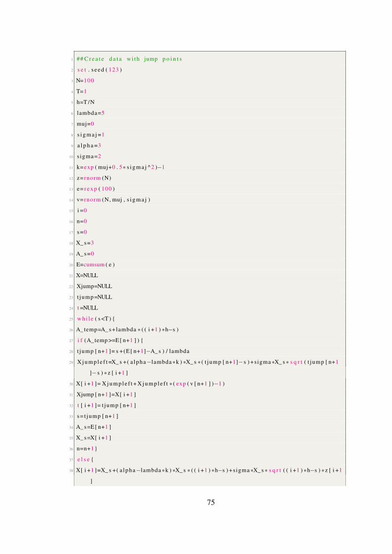
1 ## C r e a t e d a t a wi th jump p o i n t s

2 s e t . s eed ( 123 )

3 N=100

4 T=1

5 h=T /N

6 lambda=5

7 muj=0

8 s i g m a j =1

9 a l p h a =3

10 s igma=2

11 k=exp ( muj+0 . 5* s i g m a j ^2 )−1

12 z=rnorm (N)

13 e= rexp ( 100 )

14 v=rnorm (N, muj , s i g m a j )

15 i =0

16 n=0

17 s=0

18 X_ s=3

19 A_ s=0

20 E=cumsum ( e )

21 X=NULL

22 Xjump=NULL

23 t jump =NULL

24 t =NULL

25 w h i l e ( s <T )

26 A_ temp=A_ s+lambda * ( ( i +1 ) *h−s )

27 i f (A_temp >=E [ n+1 ] )

28 t jump [ n+1 ]= s +(E [ n+1]−A_ s ) / lambda

29 X j u m p l e f t =X_ s +( a lpha−lambda *k ) *X_ s *( t jump [ n+1]− s ) +sigma *X_ s * s q r t ( t jump [ n+1

]− s ) * z [ i +1 ]

30 X[ i +1 ]= X j u m p l e f t + X j u m p l e f t * ( exp ( v [ n+1 ] )−1 )

31 Xjump [ n+1 ]=X[ i +1 ]

32 t [ i +1 ]= t jump [ n+1 ]

33 s= t jump [ n+1 ]

34 A_ s=E [ n+1 ]

35 X_ s=X[ i +1 ]

36 n=n+1

37 e l s e

38 X[ i +1 ]=X_ s +( a lpha−lambda *k ) *X_ s * ( ( i +1 ) *h−s ) +sigma *X_ s * s q r t ( ( i +1 ) *h−s ) * z [ i +1

]

75

39 s =( i +1 ) *h

40 t [ i +1 ] = ( i +1 ) *h

41 A_ s=A_ temp

42 X_ s=X[ i +1 ]

43 i = i +1

44 d a t a = d a t a . f rame ( t ,X)

45 co lnames ( d a t a ) =c ( " t ime " , " v a l u e " )

46

47 l i b r a r y ( g g p l o t 2 )

48 l i b r a r y ( t i k z D e v i c e )

49

50 ## P l o t t h e d a t a ##

51 l i b r a r y ( g g p l o t 2 )

52 t i k z ( " Jump_ d e t e c t i o n . t e x " , wid th =5 , h e i g h t =5 )

53 g g p l o t ( da t a , a e s ( x= t ime , y= v a l u e ) ) +geom_ l i n e ( )

54 dev . o f f ( )

Listing A.4: Jump Detection R Script

1 d a t a = r e a d . t a b l e ( " d10 . t x t " , h e a d e r =TRUE)

2 Y= d a t a [ , 2 ]

3 X= d a t a [ , 1 ]

4 Sys . s e t l o c a l e ( "LC_TIME" , " E n g l i s h " )

5 # ######################################################

6 ## produce t h e graph of d a t a ##

7 i n s t a l l . p a c k a g e s ( " g g p l o t 2 " )

8 i n s t a l l . p a c k a g e s ( " t i k z D e v i c e " )

9 l i b r a r y ( g g p l o t 2 )

10 l i b r a r y ( t i k z D e v i c e )

11 t i k z ( " Exchangepa th . t e x " , wid th =5 , h e i g h t =3 )

12 g g p l o t ( d a t a = da ta , a e s ( x = as . Date (X, f o r m a t = ’%d.%m.%Y’ ) , y = Y) ) +geom_ l i n e

( c o l o r = " maroon " ) + s c a l e _x_ d a t e ( d a t e _ l a b e l s = "%b %Y" , b r e a k s = ’ 1 month

’ ) + x l a b ( " Time " ) + y l a b ( " " ) + theme ( l e g e n d . p o s i t i o n = " none " )

13 dev . o f f ( )

Listing A.5: Dollar to Turkish Lira Exchange Rate

76

1 d a t a = r e a d . t a b l e ( " d10 . t x t " , h e a d e r =TRUE)

2 X= d a t a [ , 2 ]

3 dx= d i f f ( l o g (X) )

4 N= l e n g t h (X)

5 T=1

6 d t =T /N

7 # ######################################################

8 ### MLE of SDE wi th Jump ###

9 dx= d i f f ( l o g (X) ) # f i n d d i f f e r e n c e o f X s t a t e s

10 f = m a t r i x ( 0 ,N−1 , 10 ) # c r e a t e empty m a t r i x f o r t r a n s i t i o n d e n s i t y

11 l i k e l i h o o d = f u n c t i o n ( t h e t a , dx , d t ) # c r e a t e a f u n c t i o n f o r l i k e l i h o o d

12

13 Q1= t h e t a [ 1 ] # s y m b o l i z e a l p h a p a r a m e t e r

14 Q2= t h e t a [ 2 ] # s y m b o l i z e sigma p a r a m e t e r

15 Q3= t h e t a [ 3 ] # s y m b o l i z e muj p a r a m e t e r

16 Q4= t h e t a [ 4 ] # s y m b o l i z e s i g m a j p a r a m e t e r

17 Q5= t h e t a [ 5 ] # s y m b o l i z e lambda p a r a m e t e r

18 k=exp ( (Q3 ) +0 . 5 * (Q4 ) ^2 )−1

19 # a s s i g n e l e m e n t o f t r a n s i t i o n d e n s i t y m a t r i x f o r N e l e m e n t s and k jump

p o s s i b i l i t i e s .

20 f o r ( i i n 1 :N−1 )

21 f o r ( j i n 1 : 10 )

22 f [ i , j ] = ( exp(−Q5* d t ) * (Q5* d t ) ^ ( j−1 ) / f a c t o r i a l ( j−1 ) ) * ( 1 / s q r t ( 2* p i * (Q2^2* d t +( j

−1 ) *Q4^2 ) ) ) * exp (−( dx [ i ] − ( (Q1−Q5*k−Q2^2 / 2 ) * d t +( j−1 ) *Q3 ) ) ^2 / ( 2 * (Q2^2* d t +(

j−1 ) *Q4^2 ) ) )

23 R=rowSums ( f )

24 LL=−sum ( l o g (R) ) # f i n d − l o g l i k e l i h o o d

25 r e t u r n ( LL )

26 l i k e l i h o o d ( c ( 1 , 1 , 1 , 1 , 1 ) , dx , d t )

27 ## Minimize − l o g l i k e l i h o o d f u n c t i o n ##

28 e s t i m a t i o n = opt im ( c ( 1 , 1 , 1 , 1 , 1 ) , l i k e l i h o o d , g r =NULL, dx , dt , method=" Nelder−Mead"

, h e s s i a n =T )

29 o p t i o n s ( s c i p e n =999 )

30 e s t i m a t i o n $ p a r

31 AIC=−2* l i k e l i h o o d ( c ( 1 , 1 , 1 , 1 , 1 ) , dx , d t ) +2*5

Listing A.6: Merton Jump Diffusion Model Parameter Estimations For Exchange

Rate

77

1 d a t a = r e a d . t a b l e ( " d10 . t x t " , h e a d e r =TRUE)

2 X= d a t a [ , 2 ]

3 N= l e n g t h (X)

4 T=1

5 d t =T /N

6 dx= d i f f ( l o g (X) ) # f i n d d i f f e r e n c e o f X s t a t e s

7 f = m a t r i x ( 0 ,N−1 , 1 ) # c r e a t e empty m a t r i x f o r t r a n s i t i o n d e n s i t y

8 l i k e l i h o o d _ bs<− f u n c t i o n ( t h e t a , dx , d t )

9

10 Q1<− t h e t a [ 1 ]

11 Q2<− t h e t a [ 2 ]

12 f o r ( i i n 1 :N−1 )

13

14 f [ i ] = ( 1 / ( s q r t ( 2* p i *Q2^2* d t ) ) ) * exp (−( dx [ i ]−Q1* d t ) ^2 / ( 2 * (Q2^2 ) * d t ) )

15

16 LL=−sum ( l o g ( f ) ) # f i n d − l o g l i k e l i h o o d

17 r e t u r n ( LL )

18

19 l i k e l i h o o d _ bs ( c ( 1 , 1 ) , dx , d t )

20 ## Minimize − l o g l i k e l i h o o d f u n c t i o n ##

21 e s t i m a t i o n = opt im ( c ( 1 , 1 ) , l i k e l i h o o d _ bs , g r =NULL, dx , dt , method=" Nelder−Mead" ,

h e s s i a n =T )

22 o p t i o n s ( s c i p e n =999 )

23 e s t i m a t i o n $ p a r

24 AIC=−2* l i k e l i h o o d _ bs ( c ( 1 , 1 ) , dx , d t ) +2*2

Listing A.7: Black-Scholes Model Parameter Estimations For Exchange Rate

78

1 a l p h a =0 . 238 # i n s t a n t a n e o u s e x p e c t e d r e t u r n

2 s igma=0 . 063 # v o l a t i l i t y o f a s s e t

3 muj=−0 . 015 # e x p e c t e d v a l u e f o r d i s t r i b u t i o n o f jump s i z e

4 s i g m a j =0 . 058 # s t a n d a r d d e v i a t i o n f o r d i s t r i b u t i o n o f jump s i z e

5 lambda=4 . 44 # jump i n t e n s i t y

6 k=exp ( muj+0 . 5* s i g m a j ^2 )−1 #mean of r e l a t i v e jump s i z e

7 M=1 # number o f p a t h s

8 Xs=5 . 82 # s t a r t i n g v a l u e f o r p r o c e s s o f X

9 N=9 # number o f o b s e r v a t i o n s

10 d t =1 / 121

11 dw= m a t r i x ( 0 ,N,M) # c r e a t e empty m a t r i x f o r dw

12 w= m a t r i x ( 0 ,N,M) # c r e a t e empty m a t r i x f o r w

13 t = seq ( dt , 1 , d t )

14 s e t . s eed ( 718 )

15 ## s t o c h a s t i c i n c r e m e n t o f Brownian p r o c e s s ##

16 f o r ( i i n 1 :M)

17 dw [ , i ]= s q r t ( d t ) * rnorm (N)

18 ## c u m u l a t i v e s t o c h a s t i c i n c r e m e n t o f Brownian p r o c e s s ##

19 f o r ( i i n 1 :M)

20 w[ , i ]= cumsum ( dw [ , i ] )

21 ## c r e a t e jump p a r t ##

22 Jump= m a t r i x ( 0 ,N,M) # c r e a t e empty m a t r i x f o r jump s i z e

23 Cumjump= m a t r i x ( 0 ,N,M) # c r e a t e empty m a t r i x f o r c u m u l a t i v e jump s i z e

24 X= m a t r i x ( 0 ,N,M) # c r e a t e empty m a t r i x f o r p r o c e s s o f X

25 dN= m a t r i x ( 0 ,N,M) # c r e a t e empty m a t r i x f o r P o i s s o n i n c r e m e n t

26 # c o n s t r u c t i n g P o i s s o n p r o c e s s #

27 f o r ( j i n 1 :M)

28 f o r ( i i n 1 :N)

29 dN [ i , j ]= r p o i s ( 1 , lambda * d t ) # d e f i n e N numbers from P o i s s o n ( lambda * d t )

30

31 # a c c o r d i n g t o e x i s t i n g o f jump , d e s c r i b e jump s i z e s

32 f o r ( j i n 1 :M)

33 f o r ( i i n 1 :N)

34 i f ( dN [ i , j ]== 1 ) Jump [ i , j ]= rnorm ( 1 , muj , s i g m a j ) # d e f i n e t h e jump s i z e s

35 e l s e

36 Jump [ i , j ]= 0 # t h e r e e x i s t no jump t h e n jump s i z e i s 0

37

38 f o r ( i i n 1 :M)

39 Cumjump [ , i ]= cumsum ( Jump [ , i ] ) # d e f i n e c u m u l a t i v e v a l u e s f o r jump s i z e s .

40 ## c o n s t r u c t i n g a n a l y t i c a l s o l u t i o n ##

79

41 f o r ( i i n 1 :N)

42 f o r ( j i n 1 :M)

43 X[ i , j ]= Xs* exp ( ( a lpha−0 . 5* sigma ^2−lambda *k ) * t [ i ]+ sigma *w[ i , j ]+ Cumjump [ i , j ] )

44 Y= m a t r i x ( c ( 5 . 76 , 5 . 81 , 5 . 80 , 5 . 78 , 5 . 77 , 5 . 79 , 5 . 74 , 5 . 65 , 5 . 65 ) ,N,M) # a c t u a l

v a l u e s

45 sum ( abs (X−Y) /Y) /N*100 # Give MAPE v a l u e

Listing A.8: Dollar to Turkish Lira Exchange Rate Merton Prediction

1 mu=0 . 112# i n s t a n t a n e o u s e x p e c t e d r e t u r n

2 s igma=0 . 114 # v o l a t i l i t y o f a s s e t

3 M=1 # number o f p a t h s

4 Xs=5 . 8214 # s t a r t i n g v a l u e f o r p r o c e s s o f X

5 N=9 # number o f o b s e r v a t i o n s

6 d t =1 / 121

7 dw= m a t r i x ( 0 ,N,M) # c r e a t e empty m a t r i x f o r dw

8 w= m a t r i x ( 0 ,N,M) # c r e a t e empty m a t r i x f o r w

9 t = seq ( dt , 59* dt , d t )

10 s e t . s eed ( 603 )

11 ## s t o c h a s t i c i n c r e m e n t o f Brownian p r o c e s s ##

12 f o r ( i i n 1 :M)

13 dw [ , i ]= s q r t ( d t ) * rnorm (N)

14 ## c u m u l a t i v e s t o c h a s t i c i n c r e m e n t o f Brownian p r o c e s s ##

15 f o r ( i i n 1 :M)

16 w[ , i ]= cumsum ( dw [ , i ] )

17 X= m a t r i x ( 0 ,N,M)

18 ## c o n s t r u c t i n g a n a l y t i c a l s o l u t i o n ##

19 f o r ( i i n 1 :N)

20

21 f o r ( j i n 1 :M)

22

23 X[ i , j ]= Xs* exp ( ( mu−0 . 5* sigma ^2 ) * t [ i ]+ sigma *w[ i , j ] )

24 Y= m a t r i x ( c ( 5 . 76 , 5 . 81 , 5 . 80 , 5 . 78 , 5 . 77 , 5 . 79 , 5 . 74 , 5 . 65 , 5 . 65 ) ,N,M) # A c t u a l

v a l u e s

25 sum ( abs (X−Y) /Y) /N*100 #MAPE v a l u e

Listing A.9: Dollar to Turkish Lira Exchange Rate Black-Scholes Prediction

80

1 d a t a = r e a d . t a b l e ( " d10 . t x t " , h e a d e r =TRUE)

2 q1= d a t a [ , 2 ][− l e n g t h ( d a t a [ , 2 ] ) ]

3 q2= d a t a [ , 2 ][−1 ]

4 b= l o g ( q2 / q1 )

5 d t =1 / l e n g t h ( l e n g t h ( d a t a [ , 2 ] ) )

6

7 # ######### Jump D e t e c t i o n ##########

8 e p s i l o n =0 . 0125

9 c=which ( abs ( b ) > e p s i l o n )

10 i n d e x = m a t r i x ( 0 , l e n g t h ( b ) , 1 )

11 f o r ( i i n 1 : l e n g t h ( c ) )

12 i n d e x [ c [ i ] ] = 1

13 k=b−i n d e x *( b )

14 a =( k−mean ( k ) ) / sd ( k )

15 ***********************************************************

16 i n s t a l l . p a c k a g e s ( " g g p l o t 2 " )

17 l i b r a r y ( g g p l o t 2 )

18 t = seq ( 2* dt , 1 , d t )

19 d a t a 2= d a t a . f rame ( t , b )

20 co lnames ( d a t a 2 ) =c ( " Time " , " LogReturns " )

21 g g p l o t ( d a t a 2 , a e s ( x=Time , y= LogReturns ) ) +geom_ l i n e ( )

22 ************************************************************

23 # ######### Model Assumpt ions ##########

24 l i b r a r y ( t s e r i e s )

25 # ###### S t a t i o n a r i t y #######

26 kpss . t e s t ( b )

27 a d f . t e s t ( z )

28 # ###### N o r m a l i t y #######

29 s h a p i r o . t e s t ( a )

30 j a r q u e . b e r a . t e s t ( z )

31 # ###### Independency #######

32 Box . t e s t ( b , l a g = 1 )

Listing A.10: Jump Detection and Model Assumption Check

81

82

APPENDIX B

DOLLAR/TL EXCHANGE RATE DATA

Date Exchange Rate Date Exchange Rate

1.02.2019 5.2084 8.03.2019 5.4303

3.02.2019 5.2167 10.03.2019 5.4338

4.02.2019 5.2182 11.03.2019 5.4455

5.02.2019 5.1985 12.03.2019 5.4572

6.02.2019 5.2168 13.03.2019 5.4564

7.02.2019 5.2668 14.03.2019 5.4671

8.02.2019 5.2474 15.03.2019 5.4467

10.02.2019 5.2517 17.03.2019 5.449

11.02.2019 5.2779 18.03.2019 5.4683

12.02.2019 5.2516 19.03.2019 5.4764

13.02.2019 5.285 20.03.2019 5.4208

14.02.2019 5.2729 21.03.2019 5.4652

15.02.2019 5.2714 22.03.2019 5.7627

17.02.2019 5.2854 24.03.2019 5.693

18.02.2019 5.3083 25.03.2019 5.5503

19.02.2019 5.2828 26.03.2019 5.3279

20.02.2019 5.3244 27.03.2019 5.3278

21.02.2019 5.3214 28.03.2019 5.561

22.02.2019 5.3186 29.03.2019 5.5555

24.02.2019 5.3203 31.03.2019 5.5919

25.02.2019 5.3026 1.04.2019 5.4863

26.02.2019 5.3066 2.04.2019 5.605

27.02.2019 5.3136 3.04.2019 5.626

28.02.2019 5.3371 4.04.2019 5.5925

1.03.2019 5.3742 5.04.2019 5.6262

3.03.2019 5.3725 7.04.2019 5.639

4.03.2019 5.3769 8.04.2019 5.6903

5.03.2019 5.387 9.04.2019 5.6943

6.03.2019 5.4288 10.04.2019 5.6818

7.03.2019 5.4712 11.04.2019 5.7388

83

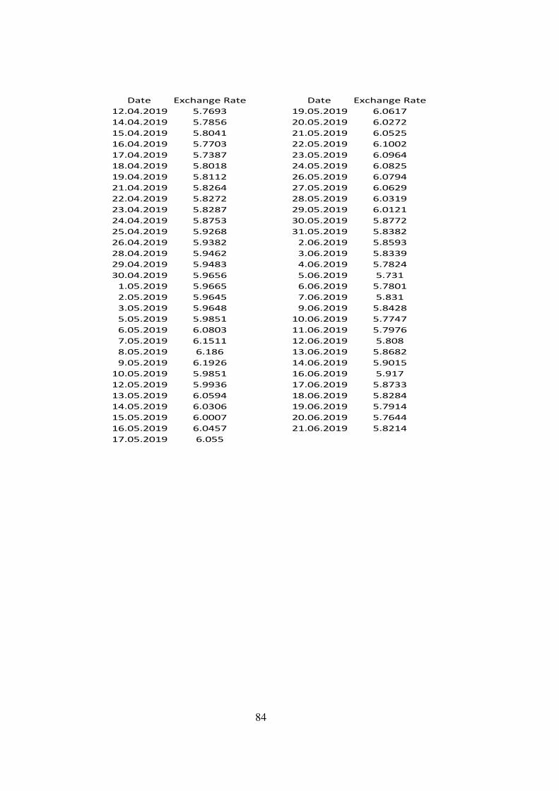
Date Exchange Rate Date Exchange Rate

12.04.2019 5.7693 19.05.2019 6.0617

14.04.2019 5.7856 20.05.2019 6.0272

15.04.2019 5.8041 21.05.2019 6.0525

16.04.2019 5.7703 22.05.2019 6.1002

17.04.2019 5.7387 23.05.2019 6.0964

18.04.2019 5.8018 24.05.2019 6.0825

19.04.2019 5.8112 26.05.2019 6.0794

21.04.2019 5.8264 27.05.2019 6.0629

22.04.2019 5.8272 28.05.2019 6.0319

23.04.2019 5.8287 29.05.2019 6.0121

24.04.2019 5.8753 30.05.2019 5.8772

25.04.2019 5.9268 31.05.2019 5.8382

26.04.2019 5.9382 2.06.2019 5.8593

28.04.2019 5.9462 3.06.2019 5.8339

29.04.2019 5.9483 4.06.2019 5.7824

30.04.2019 5.9656 5.06.2019 5.731

1.05.2019 5.9665 6.06.2019 5.7801

2.05.2019 5.9645 7.06.2019 5.831

3.05.2019 5.9648 9.06.2019 5.8428

5.05.2019 5.9851 10.06.2019 5.7747

6.05.2019 6.0803 11.06.2019 5.7976

7.05.2019 6.1511 12.06.2019 5.808

8.05.2019 6.186 13.06.2019 5.8682

9.05.2019 6.1926 14.06.2019 5.9015

10.05.2019 5.9851 16.06.2019 5.917

12.05.2019 5.9936 17.06.2019 5.8733

13.05.2019 6.0594 18.06.2019 5.8284

14.05.2019 6.0306 19.06.2019 5.7914

15.05.2019 6.0007 20.06.2019 5.7644

16.05.2019 6.0457 21.06.2019 5.8214

17.05.2019 6.055

84