parameter estimation for coupled multivariable error models

INTERNATIONAL JOURNAL OF ADAPTIVE CONTROL AND SIGNAL PROCESSING

Int. J. Adapt. Control Signal Process. 13, 145—159 (1999)

PARAMETER ESTIMATION FOR COUPLEDMULTIVARIABLE ERROR MODELS

GANG TAO* AND YI LING

Department of Electrical Engineering, University of Virginia, Charlottesville, VA 22903, U.S.A.

SUMMARY

An adaptive algorithm is developed for estimating the parameters of a linear multivariable error model withcoupled dynamics, using estimation errors for coupling inputs. Coupled dynamics in an error equation leadto a new type of error models which have different regressors but the same parameter error. A total costfunction is used to derive a desired adaptive law for updating the parameter estimates. As an application, thisalgorithm is employed for control and identification of multivariable systems with actuator uncertainties.Copyright ( 1999 John Wiley & Sons, Ltd.

1. PROBLEM STATEMENT

In the literature of parameter estimation for multivariable systems,1~5 a commonly seen errormodel is

e (t)"#3 T(t)f(t) (1)

where e(t)3Rm and f(t)3Rq are measured vector signals, and #3 (t)"# (t)!#*3Rq]m, with#(t) being the estimate of the unknown parameter matrix #*. This error model is decoupled inthe sense that the ith component of e (t), denoted as e

i(t), and the ith column of #3 (t), denoted as

hIi(t)3Rq, satisfy the condition

ei(t)"hI T

i(t)f (t) (2)

for i"1, 2,2 , m, where hIi(t)"h

i(t)!h*

ifor h

i(t) and h*

ibeing the ith columns of #(t) and #*,

respectively. It is clear that the problem of designing an adaptive law for updating the parameterestimate #(t) for the error model (1) is equivalent to that for the error model (2).

¹his paper was recommended for publication by editor C. Cowan

*Correspondence to: Gang Tao, Department of Electrical Engineering, University of Virginia, Charlottesville, VA 22903,U.S.A. Email: [email protected]

Contract/grant sponsor: National Science FoundationContract/grant number: ECS-9619363

Received 9 December 1997CCC 0890—6327/99/030145—15$17)50 Revised 26 September 1998Copyright ( 1999 John Wiley & Sons, Ltd. Accepted 11 December 1998

In some multivariable parameter estimation problems, the error model is not as simple as thatin (1). For example, e

i(t) may also depend on hI

j(t) for some jOi. To show this difference, we first

consider the single-variable error equation

e4(t)"w(D) [hI Tu](t) (3)

where e4(t)3R is a measured error signal such as a tracking error in model reference adaptive

control,6,7 u (t)3Rq is a measured vector signal, w(D) is a stable and strictly proper transferfunction, and hI (t)"h(t)!h*3Rq with h (t) being the estimate of the unknown parameter vectorh*. We note that the symbol D, as the case may be, denotes the Laplace transform variable s or thetime differentiation operator D[x](t)"xR (t) in continuous time, or denotes the z-transformvariable z or the time advance operator D[x](t)"x(t#1) in discrete time. Using this unifiednotation, we present both the continuous- and discrete-time results. As a notation, w (D) [hI Tu](t)is used to express the output of the system operator w (D) with the input hI T(t)u(t).

To develop an adaptive update law for h (t), as in References 6 and 7 an estimation error isintroduced:

e4(t)"e

4(t)#m

4(t) (4)

where the auxiliary signal m4(t) is

m4(t)"hT(t)f(t)!w(D) [hTu](t) (5)

with f (t)"w (D) [u](t)3Rq. Substituting (4) and (5) in (3), we obtain

e4(t)"hI T(t)f (t) (6)

which is exactly the single-variable version of (1). An important property of the signal m4(t) is that

m4(t)"0 if h(t)"h is a constant vector. This property is desirable for the adaptive system whose

objective is to drive the error e4(t) to zero asymptotically, because under certain signal boundness

condition the standard gradient adaptive law

hQ (t)"!

!e4(t)f(t)

1#fT(t)f (t), !"!T'0 (7)

for the error model (6) in continuous time, can asymptotically drive e4(t) to zero and h (t) to almost

a constant vector: limt?=

e4(t)"0 and lim

t?=hQ (t)"0.

To see the difference between a single-variable case and a multivariable case, we present themultivariable version of the error equation (3) as

e (t)"¼(D) [#3 Tu](t) (8)

where e(t)3Rm is a measured vector error signal such as a tracking error in multivariable modelreference adaptive control,8 u(t)3Rq is a measured vector signal, ¼ (D) is a stable and strictlyproper m]m transfer matrix, and #3 (t)"# (t)!h*3Rq]m with # (t) being the estimate of theunknown parameter matrix #*, as similar to that in (1). It is clear from (8) that the ith componentof e (t), denoted as e

i(t), depends not only on the ith column of #3 (t), denoted as hI

i(t)"h

i(t)!h*

ifor h

i(t) and h*

ibeing the ith columns of #(t) and #*, respectively, but also on other components

146 GANG TAO AND YI LING

Int. J. Adapt. Control Signal Process. 13, 145—159 (1999)Copyright ( 1999 John Wiley & Sons, Ltd.

of #3 (t). Hence, due to the interactions between different input signals, the parameter estimationproblem for multivariable systems with dynamic coupling is different from that for the single-variable case (3) for which the estimation error e

4(t) in (4) with the simple auxiliary signal m

4(t) in

(5) leads to the suitable adaptive law (7).The goals of this paper are to develop a desired adaptive law to update the estimate # (t) in the

error model (8) and to apply the developed adaptive law to control and identification ofmultivariable systems with actuator uncertainties such as dead zones, backlash or hysteresis.

In Section 2, we introduce a new auxiliary signal m (t) for a coupled estimation error. Our newauxiliary signal m(t) has the desired property that m(t)"0 if # (t)"# is a constant matrix. Weshow that a proper error model for (8) is a coupled one in the sense that a component of theestimation error may depend on many (or even all) columns of the parameter matrix #(t). InSection 3, we propose a solution to the problem of estimating the parameters of a coupledmultivariable error model. One solution employs a proper measure of the error components andretains the error model’s linearity. Based on a total cost function for the coupled error model, wedevelop an adaptive update law with desired properties for the error model’s parameters. InSection 4, we apply our new parameter estimation algorithm to control of multivariable systemswith actuator non-linear uncertainties such as dead zones, backlash or hysteresis. Our controlscheme employs an adaptive inverse to cancel the actuator uncertainties and also provides analgorithm for identifying the parameters of the actuator non-linearity. With simulation results, weshow that the improved system performance is achieved by the adaptive inverse controller.

2. COUPLED ERROR MODEL

Let us now consider the multivariable error equation (8):

e(t)"¼(D) [#3 Tu](t) (9)

Let wij(D), i, j"1, 2,2 , m, be the ijth component of the stable and strictly proper m]m transfer

matrix ¼ (D). Then, the ith component of e(t) is

ei(t)"w

i1(D) [hI T

1u](t)#2#w

im(D) [hI T

mu] (t), i"1, 2,2 , m (10)

where hIj(t)"h

j(t)!h*

j, j"1, 2,2 , m, are the jth column of #3 (t)"# (t)!#*.

For i, j"1, 2,2, m, introducing the auxiliary signals

mij(t)"hT

j(t)f

ij(t)!w

ij(D) [hT

ju] (t) (11)

fij(t)"w

ij(D) [u](t) (12)

we define the estimation errors

ei(t)"e

i(t)#m

i1(t)#2#m

im(t). (13)

Substituting (10)— (12) in (13), we obtain

ei(t)"hI T

1(t)f

i1(t)#2#hI T

m(t)f

im(t) (14)

Clearly, for i, j"1, 2,2 , m, the signals mij(t) have the desired property that m

ij(t)"0 for

hj(t)"h

jbeing constant. However, it follows from (14) that the estimation error e

i(t), measured

COUPLED MULTILINEAR VARIABLES 147


from (13), depends on hj(t) for j"1, 2,2 , m. In a compact notation, defining

hI (t)"h(t)!h* (15)

h(t)"(hT1(t) ,2 , hT

m(t))T3Rmq (16)

h*"(h*T1

,2 , h*Tm

)T3Rmq (17)

fi(t)"(fT

i1(t) ,2, fT

im(t))T3Rmq (18)

we express (14) as

ei(t)"hI T (t)f

i(t), i"1, 2,2, m. (19)

We see that the dynamic coupling in the multivariable error equation (9) leads to a set ofm estimation errors which all contain the overall system parameter vectors h (t) and h*.

The objective of parameter estimation is to update the parameter estimate h (t) so that,in addition to the boundedness of h (t), the parameter derivative hQ (t) in continuous time orthe parameter variation h (t#1)!h(t) in discrete time, and the normalized estimationerrors e

i(t)/n (t) , i"1, 2,2, m, all have finite energy, where n(t) is a normalization signal to be

defined.

3. ADAPTIVE PARAMETER UPDATE LAWS

In this section, we first develop an adaptive law for updating the parameter estimate h (t) for theerror model (19). We then present two special cases of the developed adaptive law.

3.1. Adaptive Design

To develop an adaptive law for the error model (19), we first define the cost function

J (h)"12EeE2

p"1

2( D e

1Dp#2#D e

mDp)2@p , p*1 (20)

where, E ) Ep

is the p-norm in Rm, and

e"(e1,2, e

m)T (21)

ei"(h!h*)Tf

i"hI Tf

i, i"1, 2,2, m (22)

We should note that the cost function J (h) in (20) is a measure of the total estimation error e in(21) rather than the individual error e

iwhich has the expression (19). Such a total cost function

takes into account the dynamic coupling of the error equation (9).To design an adaptive update law using a steepest descent approach,6 we evaluate

LJ

Lh"G

EeE2~pp

(+mi/1

ep~1i

fi)

EeE2~pp

(+mi/1

sign(ei) ep~1

ifi)

if p is even

if p is odd(23)



Here we define LJ/Lh"0 for e"0. We then choose the adaptive update law for h (t):

hQ (t)"!

! (LJ/Lh)(t)

n2(t)"G

!

!n2 (t)

Ee (t)E2~pp A

m+i/1

ep~1i

(t)fi(t)B if p is even

!

!n2 (t)

Ee (t)E2~pp A

m+i/1

sign(ei(t)) ep~1

i(t) f

i(t)B if p is odd

(24)

where !"!T'0 is the adaptation gain matrix, and n (t) is the normalization signal defined as

n(t)"S1#Am+i/1

Efi(t)EpB

2@p(25)

with E ) E being any vector norm in Rq for fi3Rq, for example, the p-norm E ) E

p. When e(t)"0, we

simply set hQ (t)"0.The discrete-time version of (24) is

h (t#1)"h(t)!! (LJ/Lh)(t)

n2 (t)"G

h (t)!!

n2 (t)Ee (t)E2~p

p Am+i/1

ep~1i

(t)fi(t)B if p is even

h (t)!!

n2 (t)Ee (t)E2~p

p Am+i/1

sign(ei(t))ep~1

i(t)f

i(t)B if p is odd

(26)

where 0(!"!T)c0I, with 0(c

0(2, is the step size matrix, and n (t) is the same as in (25).

Similarly, when e(t)"0, we set h (t#1)"h (t).The update laws (24) and (26) have the following properties.

¸emma 3.1

The adaptive law (24) guarantees that

(i) h (t)3¸=;(ii) EhQ (t)E

p3¸2W¸=; and

(iii)Ee(t)E

pn (t)

3¸2W¸=.

Proof. Introducing the positive-definite function

»(hI )"12hI T!~1hI (27)

where hI (t)"h(t)!h*, using (19) and (24), we have

»Q "!

hI T(t) LJLh (t)

n2(t)"!

Ee(t)E2p

n2(t))0 (28)

which implies that h (t)3¸= and Ee(t)Ep/n (t)3¸2. Using the fact that D e

iDp)EhI EpEf

iEp, we have

Ee(t)Ep

n(t))A

D e1Dp#2#D e

mDp

Ef1Ep#2#Ef

mEpB

1@p)A

EhI EpEf1Ep#2#EhI EpEf

mEp

Ef1Ep#2#Ef

mEp B

1@p"EhI (t)E (29)



With the boundedness of h (t), (29) implies that Ee(t)Ep/n(t)3¸=. It follows from (24) that

EhQ (t)Ep)E!E

p

Ee (t)Ep

n(t)

+mi/1

Eep~1i

(t)fi(t)E

pEe(t)Ep~1

pn (t)

(30)

For e(t)O0, we have

Eep~1i

(t)fi(t)E

pEe (t)Ep~1

pn (t)

)

D ei(t) Dp~1Ef

i(t)E

pEe(t)Ep~1

pn(t)

)

Efi(t)E

pn (t)

(31)

which implies that

+mi/1

Eep~1i

(t)fi(t)E

pEe(t)Ep~1

pn (t)

is bounded. From this result and the fact that Ee (t)Ep/n (t)3¸2W¸=, using (30), we conclude that

EhQ (t)Ep3¸2W¸=. K

¸emma 3.2

The adaptive law (6) guarantees that

(i) h (t)3l=;(ii) Eh(t#1)!h (t)E

p3 l2; and

(iii)Ee(t)E

pn (t)

3l2Wl=.

Proof. Using »(hI ) defined in (27), from (26), we have

»(hI (t#1))!»(hI (t))"!

Ee(t)E2p

n2 (t) A2!(+m

i/1ep~1i

(t)fTi(t))!(+m

i/1ep~1i

(t)fi(t))

Ee (t)E2p~2p

n2 (t) B)!

Ee(t)E2p

n2 (t) A2!c0

(+mi/1

D ei(t) Dp~1Ef

i(t)E)2

Ee(t)E2p~2p

n2 (t) B)!

Ee(t)E2p

n2 (t) A2!c0

(+mi/1

D ei(t) Dp)2(p~1)@p (+m

i/1Ef

i(t)Ep)2@p

Ee(t)E2p~2p

n2 (t) B)!

Ee(t)E2p

n2 (t)(2!c

0))0, 0(c

0(2 (32)

In the second inequality above, we have used the Holder’s inequality. From (32), we have thath(t)3 l= and Ee (t)E

p/n(t)3 l2. Using (28), we have Ee (t)E

p/n (t)3l=, and using (30) with hQ (t)

replaced by h (t#1)!h (t), we have that Eh (t#1)!h (t))Ep3l2. K

So far, we have presented an adaptive law for the coupled error model (19) based on the errorequation (9). This adaptive law has the same desired properties as those of the adaptive laws for



the error models of the form (1) in the literature. With a different choice of p, one can havea different version of the adaptive law in a convenient way for a practical usage.

3.2. Two special cases

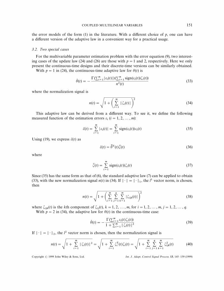
For the multivariable parameter estimation problem with the error equation (9), two interest-ing cases of the update law (24) and (26) are those with p"1 and 2, respectively. Here we onlypresent the continuous-time designs and their discrete-time versions can be similarly obtained.

With p"1 in (24), the continuous-time adaptive law for h (t) is

hQ (t)"!

! (+mi/1

D ei(t) D) (+m

i/1sign(e

i(t))f

i(t))

n2 (t)(33)

where the normalization signal is

n (t)"S1#Am+i/1

Efi(t)EB

2(34)

This adaptive law can be derived from a different way. To see it, we define the followingmeasured function of the estimation errors e

i(i"1, 2,2 , m):

eN (t)"m+i/1

D ei(t) D"

m+i/1

sign(ei(t))e

i(t) (35)

Using (19), we express eN (t) as

eN (t)"hI T (t)fM (t) (36)

where

fM (t)"m+i/1

sign(ei(t))f

i(t) (37)

Since (35) has the same form as that of (6), the standard adaptive law (7) can be applied to obtain(33), with the new normalization signal n(t) in (34). If E ) E"E ) E

1, the l1 vector norm, is chosen,

then

n (t)"S1#Am+i/1

q+j/1

m+k/1

D fijk

(t) DB2

(38)

where fijk

(t) is the kth component of fij(t), k"1, 2,2, m, for i"1, 2,2, m, j"1, 2,2 , q.

With p"2 in (34), the adaptive law for h (t) in the continuous-time case:

hQ (t)"!

!(+mi/1

ei(t)f

i(t))

1#+mi/1

Efi(t)E2

(39)

If E ) E"E ) E2, the l2 vector norm is chosen, then the normalization signal is

n (t)"S1#m+i/1

Efi(t)E2"S1#

m+i/1

fTi(t)f

i(t)"S1#

m+i/1

q+j/1

m+k/1

f2ijk

(t) (40)



4. ADAPTIVE COMPENSATION OF ACTUATOR UNCERTAINTIES

As an application of the above multivariable parameter estimation technique, we now presenta solution to adaptive compensation for actuator uncertainties in multivariable systems.

4.1. Adaptive System

Consider the multivariable plant with actuator uncertainties:

y(t)"¼(D) [u](t), u (t)"N (v(t)) (41)

where v (t), u(t), y (t)3Rm, m'1, ¼ (D) is a known m]m strictly proper rational transfer matrix,and N( ) ) represents the actuator uncertainty. Our objective is to design an adaptive compensatorto cancel the effects of N( ) ) so that the plant output y (t) tracks the desired output

yd(t)"¼(D) [u

d](t) (42)

for a given input ud(t)"(u

d1(t) ,2 , u

dm(t))T, despite the presence of the uncertainty N ( ) ). For

a simple presentation of the multivariable adaptive design for compensation of the unknownactuator non-linearities in N( ) ), we assume that the linear part ¼(D) is stable and with a goodstability margin. In our control problem, the plant output y (t) is measured, the available controlinput is v(t), while the signal u (t) is not accessible for either measurement or control.

The actuator uncertainty in each input channel is

ui(t)"N

i(v

i(t)), i"1, 2,2 , m (43)

for N( ) )"diagMN1( ) ) ,2 , N

m( ) )N, u(t)"(u

1(t) ,2 , u

m(t))T, and v(t)"(v

i(t) ,2 , v

m(t))T, and

each Ni( ) ) is parametrized by a parameter vector h*

Ni3Rn: N

i( ) )"N

i(h*

Ni; ) ).

To cancel the effects of the unknown N( ) ), we employ the adaptive inverse approach9 toconstruct an adaptive inverse NIY ( ) ) for generating the control signal v(t):

vi(t)"NI

iY (u

di(t)), i"1, 2,2, m (44)

for NIY ( ) )"diagMNI1Y (t) ,2 , NI

mY (t)N, and each inverse element NI

iY ( ) ) is parametrized by an

estimate hNi

of the unknown parameter vector h*Ni

: NIiY ( ) )"NI

iY (h

Ni; ) ), for i"1, 2,2, m.

As shown in Reference 9, an inverse NIiY ( ) ) exists for N

i( ) ) being a dead-zone, blacklash or

hysteresis. If implemented with the exact parameter vector h*Ni

, NIiY ( ) ) becomes the exact inverse:

NIi( ) )"NI

iY ( ) ) DhNi/h*

Ni(45)

which has the desired property:

ui(t)"N

i(NI

i(u

di(t)))"u

di(t), t*t

0(46)

with an initialization for backlash or hysteresis: ui(t0)"N

i(NI

i(u

di(t0)))"u

di(t0), i"1, 2,2, m,

so that the desired system performance can be achieved: y (t)"yd(t).

When implemented with a parameter estimate h*Ni

, the inverse NIiY ( ) ) leads to a control error

ui(t)!u

di(t) at each input channel:

ui(t)!u

di(t)"hI T

Ni(t)u

i(t)#d

i(t) (47)



where hINi

(t)"hNi

(t)!h*Ni

, ui(t) is a measured vector signal, and d

i(t) is a bounded error term

such that di(t)"0, t*t

0if d

i(t0)"0 and h

Ni(t)"h*

Ni, t*t

0for i"1, 2,2, m.

Define the overall parameter estimation error as

#3 T"AhI TN1

(t) 0 2 0

0 hI TN2

(t) 2 0

0 2 2 0

0 2 0 hI TNm

(t) B 3Rm]nm (48)

and the regressor vector

u"(uT1(t) ,2, uT

m(t))T3Rnm (49)

Then, the multi-channel control error is

u (t)!ud(t)"#3 T(t)u (t)#d(t) (50)

where d(t)"(d1(t) ,2 , d

m(t))T.

In view of (42) and (50), defining the tracking error

e (t)"y(t)!yd(t) (51)

we can re-express the plant (41) as

e(t)"¼ (D) [#3 Tu](t)#dM (t) (52)

where dM (t)"¼(D)d (t), and, as in (42), yd(t)"¼ (D) [u

d](t) with u

dbeing a desired input. Since

the error equation (52) is the same as that in (9) except for the bounded term dM (t), we can apply themultivariable parameter estimation technique developed in Section 3 to design an adaptive law to

update the parameter estimate # (t) to implement an adaptive inverse NIY ( ) ) for the adaptivecompensation of the actuator uncertainty N ( ) ).

To develop an adaptive law suitable for such a parameter estimation and control problem,there are two issues to be solved: one is the robustness of the adaptive laws of Section 3 withrespect to the additional term dM (t) in (52), and the other is the satisfaction of some boundarycondition on the components of the parameter estimate h

Ni, i"1, 2,2, m, needed for implemen-

ting the adaptive inverse NIY ( ) ) . A parameter projection modification9 to the adaptive law (24) or(26) is capable of solving these two issues.

It is interesting to note the special feature of the parametrization (4.10):

#3 T(t)u (t)"AhI TN1

(t)u1(t)

hI TN2

(t)u2(t)

F

hI TNm

(t)um(t) B 3Rm (53)



In view of this feature, for i, j"1, 2,2, m, we can introduce the auxiliary signals

mij(t)"hT

Nj(t)f

ij(t)!w

ij(D)[hT

Nju

j](t) (54)

fij(t)"w

ij(D) [u

j](t) (55)

and define the estimation errors

ei(t)"e

i(t)#m

i1(t)#2#m

im(t) (56)

where wij(D) is the ijth component of the stable transfer matrix ¼ (D). To use the adaptive designs

in Section 3, we also define the parameter vectors

h(t)"(hTN1

(t) ,2 , hTNm

(t))T3Rnm (57)

h*"(h*TN1

,2 , h*TNm

)T3Rnm (58)

Then, the estimation errors ei(t) can be expressed as

ei(t)"hI T(t)f

i(t)#dM

i(t), i"1, 2,2, m (59)

where dMi(t) is the ith component of dM (t), which is bounded.

The adaptive laws with parameter projection have following stability properties: h (t),Ee (t)E

p/n (t) and EhQ (t)E

pare all bounded (and so are all other signals in the adaptive system), and

that Ee(t)E2p/n2 (t), EhQ (t)E2

pand Eh(t#1)!h (t)E2

pare all bounded by EdM (t)E2

p/n2(t) in a mean

sense. The system tracking performance will be illustrated by the following simulation results forN( ) ) being a 2-channel dead zone.

4.2. Simulation Results

As an illustrative example, we consider the discrete-time two-input and two-output lineartime-invariant plant with a dead zone at each input:

y (t)"¼(D) [u](t), u (t)"DZ(v(t)) (60)

where

¼(D)"AD

(D#0)5) (D!0)8)

1

(D!0)5) (D!0)8)

D#0)6

(D#0)5)2

1

(D!0)8)2 B (61)

u (t)"DZ(v(t))"Au1(t)

u2(t)B"A

DZ1(v

1(t))

DZ2(v

2(t))B (62)

Each dead-zone element with input vi(t) and output u

i(t) is described as

ui"DZ

i(v

i)"G

mri(v

i!b

ri) for v

i*b

ri0 for b

li(v

i(b

rim

li(v

i!b

li) for v

i)b

li

(63)

where mri'0, b

ri*0, m

li'0, and b

li)0, i"1, 2, are unknown parameters.



Figure 1. Tracking errors for ud(t)"(1)5,!2)T

The structure of the dead-zone inverse DIY ( ) ) is

v(t)"Av1(t)

v2(t)B"DIY (u

d(t))"A

DIY1(u

d1(t))

DIY2(u

d2(t))B (64)

Let mliY , m

riY , m

libliY , and m

ribriY , i"1, 2 be the estimates of m

li, m

ri, m

libli

and mribri, i"1, 2,

respectively. Then each dead-zone inverse element is described by

vi(t)"DIY

i(u

di(t))"G

udi(t)#m

ribriY

mriY

for udi(t)'0

0 for udi(t)"0

udi(t)#m

libliY

mliY

for udi(t)(0

(65)

For this dead-zone problem, the control error (47) holds, with i"1, 2, for

h*Ni"h*

di"(m

ri, m

ribri, m

li, m

libli)T (66)

hNi

(t)"hdi(t)"(m

riY (t), m

ribriY (t), m

liY (t), m

libliY (t))T (67)

ui(t)"(!s

riY (t)v

i(t), s

riY (t),!s

liY (t)v

i(t), s

liY (t))T (68)



Figure 2. System responses for ud(t)"(1)5 sin(0)01t),!2)0)T



Figure 3. System responses for ud(t)"(1)5 sin(0)01t),!2 cos(0)02t))T



with the indicators functions defined as

sriY (t)"G

1

0

for vi(t)*b

riY

otherwise(69)

sliY (t)"G

1

0

for vi(t))b

liY

otherwise(70)

and di(t) is a bounded error term such that d

i(t)"0 whenever v

i(t)*b

rior v

i(t))b

li(that is, when

ui(t) and v

i(t) are outside the dead zone DZ

i( ) ); this is true if b

riY *b

riand b

liY )b

li, that is, d

i(t)

disappears if the break-points bri

and bli

are overestimated).To implement the dead-zone inverse in (46), we update

h (t)"(mr1Y (t), m

r1br1Y (t), m

l1Y (t), ml1bl1Y (t), m

r2Y (t), mr2

br2Y (t), m

l2Y (t), ml2bl2Y (t))T (71)

using the parameter estimation algorithm (19), combined with a parameter projection.9 Forsimulations, !"1.8I

8in (26), the unknown dead-zone parameter vector is

h*"(0)5, 0)5, 1)0,!0)5, 0)8, 0)536, 2)0, !0)66)T (72)

for mr1"0)5, m

l1"1, b

r1"1, b

l1"!0)5 in DZ

1( ) ), and m

r2"0)8, m

l2"2, b

r2"0)67,

bl2"!0)33 in DZ

2( ) ). The initial estimate of h* is

h (0)"(0)3, 0)3, 1)1,!0)3, 0)9, 0)36, 1)9,!0)5)T (73)

Simulations were performed for three different control schemes:

(i) the control scheme in Section 4.1 with an adaptive dead-zone inverse,(ii) the fixed dead-zone inverse control scheme with v (t)"NIY (u

d(t) implemented with the

fixed estimate h (t)"h (0) of h*, and(iii) the control scheme without dead-zone inverse: v(t)"u

d(t).

Simulation results for the first two control schemes are shown in Figures 1—3, forud(t)"(1)5,!2)T, u

d(t)"(1)5 sin(0)01t),!2)0)T, and u

d(t)"(1)5 sin(0)01t),!2 cos(0)02t))T, re-

spectively, which indicate that, with the help of an adaptive dead-zone inverse, the systemtracking errors converge to small values after a transient, while the tracking errors stay large forlarge t if no adaptation is used for a dead-zone inverse, that is, with a fixed dead-zone inverse. Theconvergence information about the estimation error e (t) and the parameter error h (t)!h* isshown in Figure 2(c) and 2(d) and in Figure 3(c) and 3(d), for the last two u

d(t).

Simulation of the third control scheme indicated that the lack of dead-zone compensation canlead to even larger tracking errors than those with a fixed dead-zone inverse controller.

5. CONCLUDING REMARKS

We presented a parameter estimation scheme for multivariable error equations with dynamiccouplings: e (t)"¼(D) [#3 Tu] (t)3Rm. We introduced auxiliary signals for the coupling terms togenerate estimation errors which lead to linearly parameterized error models: e

i(t)"hI T (t)f

i(t),

i"1, 2,2 , m, suitable for parameter adaptation but different from those commonly seen in the



literature. For the new error models with coupling parameters, we developed an adaptive law forparameter estimation which has the same desired properties as those for the single-variable case.As an application of the developed parameter estimation scheme, we designed an adaptiveactuator compensator for multivariable plants with input dead-zones, which significantly im-proves the system performance. The open issue of parameter convergence for this new parameterestimation scheme for coupled multivariable error models is currently under investigation.

REFERENCES

1. De Mathelin, M. and M. Bodson, ‘Frequency domain conditions for parameter convergence in multivariable recursiveidentification’, Automatica, 26(4), 757—767 (1990).

2. Elliott, H., W. A. Wolovich and M. Das, ‘Arbitrary adaptive pole placement for linear multi-variable systems’, IEEE¹rans. Automat. Control, 29(3), 221—229 (1984).

3. Goodwin, G. C. and K. S. Sin, Adaptive Filtering Prediction and Control, Prentice-Hall, Englewood Cliffs, NJ, 1984.4. Sastry, S. and M. Bodson, Adaptive Control: Stability, Convergence, and Robustness, Prentice-Hall, Englewood Cliffs,

NJ, 1989.5. Weller, S. R. and G. C. Goodwin, ‘Hysteresis switching adaptive control of linear multivariable systems’, Proc. 31st

IEEE CDC, Tucson, AZ, 1992, pp. 1731—1736.6. Ioannou, P. A. and J. Sun, Stable and Robust Adaptive Control, Prentice-Hall, Englewood Cliffs, NJ, 1995.7. Narendra, K. S. and A. M. Annaswamy, Stable Adaptive Systems, Prentice-Hall, Englewood Cliffs, NJ, 1989.8. Tao, G. and P. A. Ioannou, ‘Stability and robustness of model reference adaptive control schemes’, in Leondes, C. T.

(ed.), Advances in Robust Control Systems ¹echniques and Applications, Vol. 53, Academic Press, New York, 1992.9. Tao, G. and P. V. Kokotovic, Adaptive Control of Systems with Actuator and Sensor Nonlinearities, Wiley, New York,

1996.



parameter estimation for coupled multivariable error models

Documents