parallel systems in financial information processing

CONCURRENCY: PRACTICE AND EXPERIENCE, VOL. 8( lo), 741-755 (DECEMBER 1996)

Experiences in parallelising FLITE3D on the Cray T3D ROBERT M. BAXTER,' KILLIAN D. MURPHY~ AND SHARI M. TREWIN'

I EPCC, James Clerk Manveil Building, The King's Buildings, University of Edinburgh, Muyjeld Rod , Edinburgh EH9 3JZ, UK

2/ONA Technologies. Dublin, Ireland

SUMMARY FLITE3D is an unstructured multigrid Euler-CFD code, originally written by Imperial College, London, and Swansea University, and now developed by British Aerospace. In this paper we present our experiences at EPCC in porting FLITE3D to the Cray T3D MPP system. We discuss the operational requirements of a parallel production CFD code, and introduce the PUL-SM static mesh runtime library. We present performance results for the parallel FLITE3D Euler flow solver running on the UK National Supercomputing Service T3D, and echo our belief that massively parallel systems are a natural tool for commercial CFD modelling today.

1. INTRODUCTION

The ability to build accurate computational models of airflow past complex aerodynamic geometries is an increasingly important aspect of the design of modern aircraft. Commercial and competitive pressures mean that more is being demanded of CFD models: larger models, more accurate results, faster turnaround time. A natural response to these pressures is CFD modelling on massively parallel computers.

FLITE3D is a suite of CFD programs written originally by Imperial College, London, and Swansea University and now subject to continuing development within British Aerospace. It is designed to provide a complete environment for calculating steady-state Euler solutions of airflow past complex geometries. The central plank of FLITE3D is the finite-element Euler flow solver FLITE3DJ;S. This paper reviews our experiences in porting FLITE3DJ;S onto the Cray T3D MPP system. This work was a collaborative venture with British Aerospace, funded partly by them and partly by the UK Government DTI and EPSRC under the Parallel Applications Program.

In Section 2 we give an overview of the FLITE3D flow solver. In Section 3 we describe the PUL-SM runtime Static Mesh library developed at EPCC, and in Section 4 we discuss the melding of FLITE3DJ;S and PUL-SM, together with the MPI message-passing system, to give parallel FLITE3DJS. We discuss the operational requirements that drove the design choices and the reasons behind them. Section 5 presents our initial performance results for the parallel code on the Cray T3D, and Section 6 our conclusions.

2. AN OVERVIEW OF FLITE3D

As mentioned above, FLITE3D is a suite of stand-alone programs that covers a range of calculational tasks, from surface triangulation and tetrahedral mesh generation through to data post-processing.

CCC 1040-3 108/96/10074 1-1 5 01996 by John Wiley & Sons, Ltd.

Received 18 December 1995

742 R . M. BAXTER, K. D. MURPHY AND S. M. TREWIN

Our work on FLITE3D involved just two of the modules, the preprocessor, FLITE3DPP and the Euler flow solver, FLITE3DJS. The preprocessor module reads data files describing a three-dimensional unstructured tetrahedral mesh and a set of surface patches and calculates surface normals and, in the serial code, Galerkin finite element weight functions. The flow solver takes the output from the preprocessor and performs the actual flow calculation, iterating the Euler equations to a steady-state solution.

2.1. The Euler flow solver

The flow solver FLITE3D-FS provides steady-state solutions to the set of equations

au aFi a t axi - + - = o

where summation is implied over the index i, and we define the vector of unknowns

and the inviscid flux vector

We use the notation u = (u, v, w) for the three components of fluid velocity, p is the fluid density, p the pressure and E the specific total energy.

Equation (1) combines the compressible Euler equations, the continuity equation and the fluid energy equation. The equivalent finite-element equations are derived from the Galerkin weighted residual approximation over a domain R with boundary r:

NidR = F, -dS2 - FJ. Nidr J ,JZ s, (4)

where N

u*(x, t ) = 1 u~(x, t)Ni(x) (5 )

the Ni(x) are the finite element shape functions at node i and FJ. is the value of the flux normal to the domain boundary r. The analysis here follows closely that of [ 11.

If we replace the integrals over R and r by sums over the constituent elements and boundary faces, equation (4) becomes

i= 1

where e E i means ‘all elements connected to node i’, and b E i means ‘all boundary faces connected to i’. From this, we approximate the left-hand side using the lumped mass matrix

PARALLELISING FLITE3D ON THE CRAY T3D 743

M," is the diagonal approximation to the (almost) diagonal full mass matrix

For the edge-based data structures used in FLITE3D, the first term on the right-hand side of equation (6) is written

where the sum s runs over all sides emanating from node i, and the finite element weight functions for the sides, Cj, are defined as

for all elements e with volumes fle sharing side s.

that The time-integration is performed explicitly with a multistage Runge-Kutta scheme such

(10)

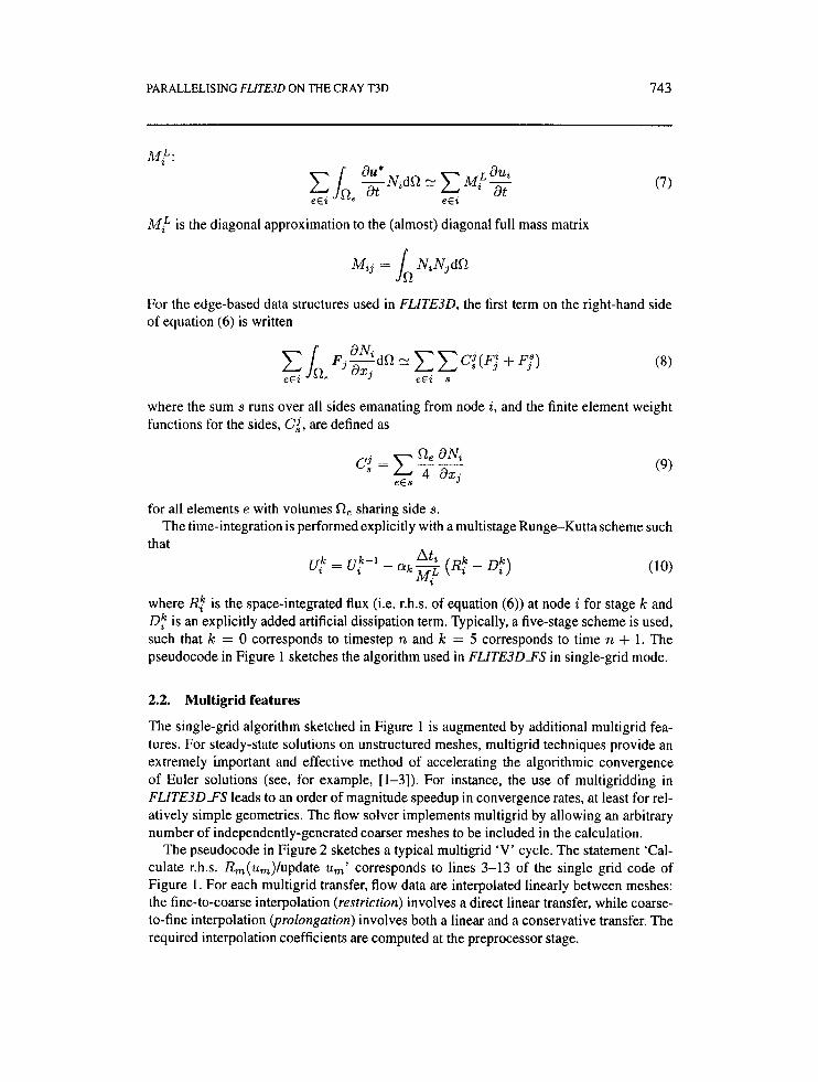
where Rf is the space-integrated flux (i.e. r.h.s. of equation (6)) at node i for stage k and 0: is an explicitly added artificial dissipation term. Typically, a five-stage scheme is used, such that k = 0 corresponds to timestep n and k = 5 corresponds to time n + 1. The pseudocode in Figure 1 sketches the algorithm used in FLITE3DYS in single-grid mode.

At, uz'" = q-' - Q k - ("; - @) M;

2.2. Multigrid features

The single-grid algorithm sketched in Figure 1 is augmented by additional multigrid features. For steady-state solutions on unstructured meshes, multigrid techniques provide an extremely important and effective method of accelerating the algorithmic convergence of Euler solutions (see, for example, [l-31). For instance, the use of multigridding in FLITE3DJS leads to an order of magnitude speedup in convergence rates, at least for rel- atively simple geometries. The flow solver implements multigrid by allowing an arbitrary number of independently-generated coarser meshes to be included in the calculation.

The pseudocode in Figure 2 sketches a typical multigrid 'V' cycle. The statement 'Cal- culate r.h.s. R,(u,)lupdate urn' corresponds to lines 3-13 of the single grid code of Figure 1 . For each multigrid transfer, flow data are interpolated linearly between meshes: the fine-to-coarse interpolation (restriction) involves a direct linear transfer, while coarse- to-fine interpolation (prolongation) involves both a linear and a conservative transfer. The required interpolation coefficients are computed at the preprocessor stage.

744 R. M. BAXTER, K. D. MURPHY AND S. M. TREWIN

Pseudo: Single-grid FLITE3DJ.Y 1. Get initial solution u

3. calculate Xt

5 . Calculate pressure. p 6. I. If (dissipation required) Then 8. 9.

10. EndIf 1 1 . Apply boundary conditions 12. Assign u = u - (Ik $Rk 13. EndFor 14. EndFor 1 5 , Write out final solution u EndPseudo

2. For n = 1, Nite tions

4. For k = 1 9 NRK-stages

Calculate integrated fluxes Rk(u, p )

Calculate dissipation Dk (u, p) Assign Rk = Rk - Dk

Figure I . FLITE3DTS single-grid algorithm

3. THE PUL-SM RUNTIME LIBRARY

The PUL-SM library [4] is a part of EPCC’s suite of Parallel Utilities Libraries, a set of runtime utilities designed to provide support for archetypal parallel programming paradigms. PUL-SM provides support to application programs which use distributed, static, irregular meshes such as are common in calculations based on finite element methods. PUL-SM is general-purpose and flexible, supporting both two- and three-dimensional meshes com- posed of arbitrary convex elements.

PUL-SM is implemented on top of the MPI message-passing interface [S] and provides facilities for the creation, initialisation, configuration and use of any number of independent

Pseudo: Multigrid FLlTE3D-F.Y 1. Get initial solution U I on finest mesh m = 1

3. While m < mcoarsest 4. Calculate r.h.s. &(um)lupdate urn 5 . m = m + l 6. Restrict u,,,-l -+ urn

8. EndWhile 9.

10. While m > 1 11. m = m - 1 12. Prolong u,+1 + urn 13. 14. EndWhile 15. EndFor 16. Write out final solution u1 Endpseudo

2. For n = 1, Nitemtions

I. Restrict Rm-1 -+ Rm

Calculate r.h.s. R,,, (um)lupdate Um

Calculate r.h.s. R,,, (u,)/update urn

Figure 2. Pseudocode outline for a multigrid ‘V’ cycle in FLITE3DIS

PARALLELKING FLITE3D ON THE CRAY T3D 745

-~

distributed meshes. Each mesh is represented by a unique instance of PUL-SM which exists within its own communication context. For each such instance, PUL-SM supports a range of mesh operations, the most pertinant of which are initial configuration, data update at local mesh boundaries and queries about the local and global mesh. The utility also provides functions to read, distribute and initialise any general mesh from a single data file, although these facilities are not used in parallel FLITE3D.

The following features illustrate some aspects of the flexibility of PUL-SM, together with the restrictions it enforces:

I .

2.

3.

4.

5.

6 .

3.1.

The size of the global mesh, and the sizes of local meshes, are not constrained by PUL-SM but only by the memory available on the underlying architecture. Mesh constituents may have any number of data items associated with them; these items may be of any user-defined type. Data may be associated with any constituent of the mesh: points, edges, faces or three-dimensional elements such as tetrahedra. Only one global mesh may be associated with any one instance of the PUL-SM utility. However, multiple instances of the utility can be used if overlaid meshes are required (for instance, in multigrid applications). A processor may participate in more than one instance of the PUL-SM utility at a given time. The processor may also participate in other PUL utilities and perform its own explicit communications without causing interference with PUL-SM. The maximum number of processors that may participate in an instance of PUL-SM is limited only by the underlying architecture. The number of mesh processors is fixed throughout the lifetime of a given istance of the utility.

Features of distributed meshes in PUL-SM

In PUL-SM, neighbouring processors may share points, edges and, in three dimensions, faces with adjoining local meshes. We use the term element to refer to the highest- dimensional constituent of a given mesh; for instance, in the case of FLITE3D, the mesh elements are tetrahedra. PUL-SM ensures that mesh elements are owned by a unique processor, and are not replicated on any other processor. Elements owned by a processor are termed local elements; all others are remote. Points shared between more than one processor are referred to as shadow points. Edges and faces made up of shadow points are also shared between processors, and are referred to as shadow edges and shadow faces, respectively. Figure 3 illustrates these features for a trivial two-dimensional mesh.

This concept of shadow constituents is used instead of data halos. For the unstructured mesh model, the implementation of data halos becomes a much more difficult proposition than for regular domain models, including the requirement for an additional (and poten- tially fairly large) fraction of storage space. The shadow constituent model requires some more interprocessor communication, but benefits from lower memory costs and conceptual simplicity.

Data on shadow constituents are updated by an operation termed a boundary swap, a joint communication/data combination operation. PUL-SM permits any data combination functions to be registered for a particular data item; the application program supplies the appropriate callback function. Typically this operation will be summation, though it need not be. Partial computations are done locally for the shadow constituents, and then the


Figure 3. Example 2-d mesh split into 2 local meshes

partial results are combined through the swap operation. Accumulating partial computations in this way exposes the danger of overcounting the

shadow constituents. For example, to calculate the number of sides emanating from each point of the mesh, we would loop over all the sides, examine the points at either end of each side and increment a counter for them both. Consider point N in Figure 3. The processor holding the left-hand side of the mesh counts four sides, as does the right-hand processor. Totalling the partial sums gives 8, while the correct result is 6; the two shadow sides have each been counted twice.

PUL-SM avoids the overcounting problem by implementing the concept of priniary and secondary mesh constituents. A constituent only ever has one processor as its primary owner, even if it is a shadow. By ordering the internal lists of mesh constituents to store all primary-owned first, overcounting can be avoided at the application level by, in the above example, looping only over primary sides. A constituent internal to the local mesh is automatically primary-owned by that processor; shadow constituents may or may not be according to an appropriately-chosen application ‘primary ownership’ function.

4.

The main reasons for parallelising FLITE3DJS for the Cray T3D were threefold: firstly, to allow larger problem meshes to be tackled, tbereby increasing calculational accuracy; secondly, to speed up large calculations by applying large numbers of processors, thus reducing turnaround time; and finally to increase throughput for problems requiring a modest number of processors. These three factors are of vital importance in the design of modern airframes in a commercial environment.

OPERATIONAL REQUIREMENTS AND PARALLEL STRATEGY


A typical operational use of FLITE3D would be to generate a mesh for a specific geometry and then run the flow solver for 15-25 different sets of flow parameters over the same geometry. The flow solver is thus the most often repeated of the FLITE3D programs, and is also, in fact, the longest to run. Consideration of these issues led us to the following design requirements:

1. Keep additional memory use to a minimum, to allow large problems to be run on

2. Ensure facilities are available to handle arbitrary numbers of independent meshes for

3. Keep the time spent in mesh initialisation and distribution to a minimum. 4. Keep code changes to a necessary minimum to facilitate ease of maintainance. 5. Facilitate future development work by using a portable message-passing environment

6. Incorporate T3D-specific optimisations wherever appropriate, activated by acompile-

With these issues in mind, the parallel FLITE3D code was designed as a generic MPI code, using PUL-SM to handle the local mesh boundary updates and general housekeeping. PUL-SM’s lack of data halos meant we could keep additional memory costs down, and its ability to handle multiple independent meshes greatly facilitated the parallelisation of the multigrid features.

One thing PUL-SM did not provide was any facility for transferring data between meshes. The multigrid interpolation operations were therefore written with explicit MPI message- passing. In addition, the mesh distribution code was tailored specifically to FLITE3D, with much of the work of distributing the mesh done in the serial preprocessor stage. A ‘ready- distributed’ mesh file, written by FLITE3DPP, could then be read quickly and easily by the flow solver.

For the preprocessor, this meant significant code changes to enable it to read in a mesh decomposition file and use the information to calculate processor ownership for all the mesh constituents. In turn, the flow solver required new code to read and distribute the new mesh file over a set of N ~ E ~ processors. The mesh distribution was designed to scale with increasing numbers of processors by implementing multiple ‘file reader’ processors - for every subgroup of 16 processors (say), one processor in the subgroup is designated the server, reads the appropriate sections of the file and distributes them within the subgroup. This scalable approach proved to be very efficient (see Section 5.2).

The largest impact on FLITE3D-FS was thus in the initialisation stage. The use of the PUL-SM swap function meant that source-code impact in the solver computation routines was small, as illustrated in Figure 4.

modest numbers of processors, to increase throughput.

multigrid operation.

rather than a T3D-specific shared memory approach.

time switch.

5.

Below we present some initial performance results for the parallel FLITE3DJS code running on the UK National Supercomputing Service Cray T3D sited at EPCC. This service comprises 384 DEC Alpha processing elements hosted by a Y/MP front-end with pre- and postprocessing facilities provided by a 10-CPU Cray J90.

Each of the superscalar Alpha processing elements (PEs) has a clock speed of 150 MHz, 64 Mbytes core memory and 8 Kbyte direct-mapped instruction and data caches. The PEs

PERFORMANCE OF PARALLEL FLITE3D ON THE CRAY T3D


Pseudo: Serial loop 1 . For S = 1, Nedges 2. 3. EndFor 4. For f = 1, Nfaces 5. 6. EndFor

Compute r.h.s. R from u and edge weights C,

Add r.h.s. contributions from boundary face f

EndPseudo

Pseudo: Parallel loop I . For s = 1 , N::gsq 2. 3. EndFor 4. For f = 1, NfmS 5. 6. EndFor 7. Do boundary swap on R

Compute r.h.s. R from u and edge weights C,

Add r.h.s. contributions from boundary face f

EndPseudo

Figure 4. Parallel changes to a typical serial loop in FLITE3DFS

are connected in a 3-dimensional torus by independent bidirectional data channels in each of the x, y and z directions. The data channels have a quoted transfer rate of 300 Mbytels.

The Alpha PEs are capable of initiating one floating-point operation per clock cycle; thus each has a notional peak performance rate of 150 MFLOPS. However, the restrictive 8K direct-mapped data cache means that, in practice, real-code performance of around 20 MFLOPS can be considered a very good benchmark figurel61'.

The datasets used for these tests were supplied by British Aerospace. They comprise three versions of the standard ONERA M6 wing, one of 200,000 tetrahedra, one of 26,000 and one of 2,000. We measured performance for both single-grid runs using the 200,000 tetrahedron mesh and multigrid runs with the 200,000 tetrahedron mesh as the finest in a three-level 'V' cycle.

The meshes were initially decomposed using the Chaco partitioning utility [7], using the multilevel recursive spectral bisection algorithm. The dualgraph used as input to Chaco was created from the FLITE3D mesh geometry files using a tool based on EPCC's PUL-MD mesh decomposition library [8].

5.1. Multigrid performance

Figure 5 shows a graphical profile of the parallel FLZTE3DJ;S code for a multigrid run of 100 iterations over eight PEs, starting with free-field flow conditions and finishing with flow residuals of order

We have broken the profile down into readingldistributing the initial mesh file, other initialisation, actual flow solution, with multigrid interpolation overheads factored out, and writing the final solution file. For this multigrid run, the initial mesh file is some 16 Mbytes in size. A key feature here is the very short time taken to read and distribute all three multigrid meshes, plus associated interpolation data. The additional initialisation costs

'An average over all user codes on the Edinburgh T3D, weighted by percentage of cycles used, gives a mean rate of 20 MFXOPS per PE

PARALLELISING FUTE3D ON THE CRAY T3D 749

Figure 5. Profile for FLITE3DJS running M6 over eight PEs

involve the calculation of the mesh edges and finite element weights, plus cell volumes and other constant arrays.

For this run of 100 multigrid cycles, the code sustained an overall workrate of 88.0 MFLOPS, or 11 .O MFLOPSPE. Table 1 shows the variation of workrates for the same 3-mesh dataset on 8, 16 and 32 PEs. In this Table we show both the overall rate for the whole FLZTE3DYS program, plus the rates for the flow solver part alone (combining the flow solution and multigrid interpolation parts of Figure 5 ) .

Table 1 . MFLOPS rates for multigrid runs of FLITE3DES, showing overall rates for the whole program and rates for the actual finite-element flow solver

FLITE3DES Solver NpEs Total Per PE Total Per PE

8 88.0 11.0 97.6 12.2 16 166.4 10.4 182.4 11.4 32 262.4 8.2 291.2 9.1

Note that the efficiency falls here as the number of processors is increased. This is due primarily to the decreasing compute workload for the (comparatively) fixed communication overhead (see Section 5.2 and Figure 8 for a deeper analysis of scaling with number of PEs) .

The communication overheads in the actual flow solver derive largely from the PUL-SM swap operation, but also include time spent in MPI reduction operations used to calculate


8000.0 - v u)

6000.0 - m 5 I-

4000.0

10000.0

-

-

-

M T3D - - _ _ Alpha 3000-400

0.0 ' L

0 8 16 24 32 40 Number of PEs

Figure 6. Comparison of total times for a 500 iteration multigrid run on both the Cray T3D and an Alpha 3000-400 workstation

the r.m.s. residuals and maximum Mach numbers every cycle. In Figure 6 we plot the total times for 500 multigrid cycles for these meshes on 8, I6 and

32 T3D PEs, compared to the time on an Alpha 3000-400. The Alpha 3000-400 uses the same chip (AXP 21064) as the T3D nodes, clocked slightly slower (133 MHz) but with a 5 12 Kbyte L2 cache against no L2 cache on the T3D.

5.2. Single-grid performance

To examine the scaling of the FLITE3DIS code with number of processors we analysed a range of single-grid runs using the finest 200,000 tetrahedron M6 dataset.

One of the most important design considerations was keeping the mesh initialisation time to a minimum, and ensuring scalability in the mesh reading and distribution. Figure 7 shows the total initialisation time and the mesh reading/distribution time against number of PEs. For the single-grid cases, the mesh file that is read is around 1 1 Mbytes in size.

At low numbers of PEs it is clear that the dominant factor is the time spent in the calculation of mesh edges and f.e. weights rather than the reading/distribution of the mesh file. As NPE~ increases, the time spent in compute overhead falls and the distribution time rises slightly. However, the gradient is shallow and even on 128 PEs the program only takes 14.4 s to complete its initialisation.

In Figure 8 we present the equiavalent graph for the Euler solver routine. In this Figure the y-axis is time per cycle of the solver, in seconds. The important feature of this graph is that the communication overhead remains fairly uniform over the range 4-128 PEs, while the time spent computing actual work falls steadily with the decreasing size of the dataset

PARALLELISING FLITE3D ON THE CRAY T3D 75 1

Figure 7. Initialisation times for single-grid M 6 runs, divided into computational overhead and mesh distribution times

(from 50,000 tetrahedra per processor on four PEs to 1560 per processor on 128). This goes a long way to explain the scaling of the MFLOPS rates in Table 1. It is clear that for 64 and I28 PEs the dataset is simply not large enough.

Table 2 presents the equivalent figures for the Euler solver routines for the single grid case. Included for comparison is the rate for the serial code on 1 PE. This rather poor serial rate gives a good indication of how hard it can be to achieve good single-node performance on the T3D; the profiler report indicates that the code spent over 64% of its time loading the instruction and data caches.

It is worth noting that a crucial factor in the flat communication times of Figure 8 is the quality of the underlying mesh decomposition. The key metric for determining the communication overhead is the number of neighbours each local mesh domain has. In Table 3 we list the lowest, highest and average numbers of neighbours per domain in the decompositions produced by Chaco running multilevel RSB.

Finally, in Figure 9 we present the total timings for 1000 iterations of the single-grid solution, along with the time on a Cray Y/MP 4E for comparison.

As can be seen, eight T3D PEs and above win out over the YMP, though the returns

152 R. M. BAXTER, K. D. MURPHY AND S . M. TREWIN

Figure 8. Times per cycle for the Eulerflow solver, divided into compute and communication times

diminish above 32 PEs because of the falling local dataset size. By comparison, the equivalent time for a single-PE run of the serial code would be 41,700 s, or 1 1 h. This figure is based on a scaling up from a 10 iteration run, using the expression

If we calculate speedup figures from these results using the formula

Ti Speedup for N processors, SN 3 - T N

then we obtain Figure 10.

5.3. Discussion

We feel that the super-linear speedup between 4 and 64 processors can be largely explained as a caching issue. The T3D Alpha nodes suffer from the small 8 Kbyte, direct-mapped L1 cache and no L2 cache. As noted above, the serial program spends over 64% of its


0.0 ' I

Figure 9. Comparison of total times for a 1000 iteration single-grid run on both the Cray T3D and Cray Y/MP 4E

time loading either instruction or data cache. The massive gains in the parallel code derive largely from the reduction in the size of the per-PE dataset. Of course, there is a turnaround point when the local dataset becomes too small to justify the necessary communication overhead. This can be seen to happen somewhere between 64 and 128 PEs. There is a clear lesson here that performance on the T3D depends on single-node code optimisations, particularly cache use.

An unfortunate feature of unstructured mesh codes is the poor locality-in-memory of the data. Calculations involve indirect array addressing of long, unstructured lists - not the most 'cache-friendly' programming model. The above comments about the T3D cache apply equally to any scalar RISC-based processor; thus a prime aim for further code optimisations would be improving the memory-locality of the local mesh data. We would expect this to yield good performance gains on such processors, and the T3D in particular.

Further analysis is needed to establish the optimum operational configuration for a given dataset, but judging by the data of Table 2 a per-PE dataset size of around 25,000 tetrahedra is a reasonable rule-of-thumb for efficient code performance. Given that the communication costs remain fairly constant as N ~ E ~ is increased, it is not unreasonable to project that a 3.2 million tetrahedra dataset could sustain N 1.5 GFLOPS on 128 PEs.

6. CONCLUSIONS

In porting FLZTE3D to the Cray T3D, our key conclusion has been that the main effort of parallelisation falls not in the flow solver code but in the preprocessing and the mesh distribution. Use of library routines such as PUL-SM can prove extremely convenient in parallelising an existing serial code; the difficult part lies in partitioning and distributing the unstructured mesh over the processor group.


Table 2. MFLOPS rates for the finite-element Euler solver on single-grid runs of FLfTE3DSS

Solver N p h Total Per PE

1 7.2 7.2 4 49.2 12.3 8 106.4 13.3

16 188.8 11.8 32 352.0 11.0 64 524.8 8.2

128 691.2 5.4

The performance results for the parallel FLITE3DJS code are extremely encouraging, indicating at the very least that it is viable as a production code. Perhaps the best feature of the parallel results is that the communication overhead in the Euler solver scales almost as a constant against increasing N P E ~ . This benign scaling of communications assists us in obtaining the ‘superlinear’ speedup observed all the way up to 64 PEs; again, we stress the importance of good-quality mesh decompositions in achieving this behaviour.

The T3D code compares well against the alternative serial platforms, with eight PEs beating the Y/MP time by around 20%. The major advantage the T3D has is one of memory scalability; memory models of the FLJTE3D3;S code suggest that a 256-PE T3D with 64 Mbytes per PE should be able to handle40 million tetrahedra in combined multigrid meshes. Our work indicates that MPP platforms have a definite place in today’s world of commercial aerodynamic design.

100.0

CL 1 D

01

6 50.0

0.0

Number of PEs

Figure 10. Speedup curve for single-grid M6 runs on the T3D. The dashed line indicates linear speedup

PARALLELISING FLlTE3D ON THE CRAY T3D 755

Table 3. Numbers of neighbouring domains in the Chaco decompositions used in this analysis

Nos. of neighbouring domains N P E ~ Lowest Highest Mean

4 3 3 3.0 8 6 7 6.5

16 2 13 8.4 32 3 20 9.0 6 4 3 26 11.1

128 5 29 12.6

ACKNOWLEDGEMENTS

The authors would like to acknowledge the support of British Aerospace and the UK DTI and EPSRC in funding this work. In addition, we wish to thank the many support staff on the EPCC T3D for maintaining an excellent level of service. Finally, thanks to Simon Chapple and Julian Parker of EPCC for their advice and valuable contributions to this project.

REFERENCES I . J. Peir6 J. Peraire and K. Morgan, ‘Finite element multigrid solutions of Euler flows past installed

aero-engines’, Comput. Mech., 11,433451 (1993). 2. J. Peir6 J. Peraire and K. Morgan, ‘A 3D finite-element multigrid solver for the Euler equations’,

Technical Report 92-0449, AIAA, January 1992. 3. D. J. Mavriplis, ‘Three dimensional unstructured multigrid for the Euler equations’, AIAA J . , 30,

4. S. M. Trewin, ‘PUL-SM prototype user guide’, TechnicalReport EPCC-KTP-PUL-SM-PROT-UG 0.2, Edinburgh Parallel Computing Centre, February 1995.

5. Message Passing Interface Forum, MPI: A Message-Passing Interfnce Standard, May 1994. 6. S. P. Booth, T3D In-Depth Support Manager, Private communication. 7. B. Hendrickson and R. Leland, ‘The Chaco user’s guide’, Technical Report SAND93-2339, Sandia

National Laboratories, November 1993. 8. S. M. Trewin, ‘PUL-MD prototype user guide’, Technical Report EPCC-KTP-PUL-MD-PROT-

UG 0.3, Edinburgh Parallel Computing Centre, June 1995.

(7), 1753-1761 (1992).

parallel systems in financial information processing

Documents