Parallel relative radiometric normalisation for remote sensingimage mosaics

Chong Chen, Zhenjie Chen n, Manchun Li, Yongxue Liu, Liang Cheng, Yibin RenJiangsu Provincial Key Laboratory of Geographic Information Science and Technology, Nanjing University, No. 163, Xianlin Avenue, Nanjing 210023, China

a r t i c l e i n f o

Article history:Received 19 December 2013Received in revised form22 July 2014Accepted 18 August 2014Available online 23 August 2014

Keywords:MosaicRelative radiometric normalisationIR-MADParallel computingRemote sensing

a b s t r a c t

Relative radiometric normalisation (RRN) is a vital step to achieve radiometric consistency amongremote sensing images. Geo-analysis over large areas often involves mosaicking massive remote sensingimages. Hence RRN becomes a data-intensive and computing-intensive task. This study implements aparallel RNN method based on the iteratively re-weighted multivariate alteration detection (IR-MAD)transformation and orthogonal regression. To parallelise the method of IR-MAD and orthogonalregression, there are two key problems: the normalisation path determination and the task dependenceon normalisation coefficients calculation. In this paper, the reference image and normalisation paths aredetermined based on the shortest distance algorithm to reduce normalisation error. Formulas oforthogonal regression are acquired considering the effect of the normalisation path to reduce the taskdependence on the calculation of coefficients. A master-slave parallel mode is proposed to implementthe parallel method, and a task queue and a process queue are used for task scheduling. Experimentsshow that the parallel RRN method provides good normalisation results and favourable parallel speed-up, efficiency and scalability, which indicate that the parallel method can handle large volumes ofremote sensing images efficiently.

& 2014 Elsevier Ltd. All rights reserved.

1. Introduction

In remote sensing applications, there is an increasing need toanalyse remote sensing data over large areas, which involvesmosaicking massive remote sensing images. Geo-analysis withremote sensing images is often conducted under the conditionthat the images are radiometrically consistent. As remote sensingimages are acquired on different dates and different environmen-tal or sensor conditions, relative radiometric normalisation (RRN)is routinely implemented to minimise radiometric differencesamong images. The RRN method applies one image as a referenceand adjusts the radiometric properties of the subject images tomatch the reference image (Hall et al., 1991). Mosaicking a largearea requires the processing of a number of adjacent images; thusthe RRN process is a computing-intensive and time consumingtask. In recent years, emerging parallel hardware architecture,such as computer clusters and multi-core processes, offers oppor-tunity to enhance the performance of the processing of rasterimages (Valencia et al., 2007; Lee et al., 2011; Guan et al., 2012;Maulik and Sarkar, 2012; Van Den Bergh et al., 2012). To meet the

demands of rapid radiometric normalisation of remote sensingimages for mosaicking, it is necessary to implement RRN methodsin parallel framework.

A few studies have been performed on the parallelisation ofmosaicking (An et al., 2002; Wang et al., 2010; Chen et al., 2011;Wu et al., 2013). Most of them use histogram matching forradiometric normalisation because the process of histogrammatching for each subject image is independent and can be easilyparallelised. Although histogram matching is useful to match dataof the same scene acquired on different dates with slightlydifferent sun angles or atmospheric effects (Yang and Lo, 2000),it is not useful for assembling several images into a mosaic becausethey do not have common constant reflectance targets(Shimabukuro et al., 2002). Typically, the RRN methods used formosaicking utilise a linear comparison of statistical characteristicsof overlaps between adjacent images to derive gains and offsetsfrom pseudo-invariant features (PIFs) (Hall et al., 1991; Du et al.,2002; Olthof et al., 2005; Paolini et al., 2006; Canty and Nielsen,2008). Canty et al. (2004) demonstrated a successful example ofmosaicking by automatically selecting invariant pixels betweenimages using the multivariate alteration detection (MAD) techni-que (Nielsen et al., 1998). This mosaicking technique selectsinvariant pixels automatically except a decision threshold, andprovides a favourable result with other manual methods (Schmidt

Contents lists available at ScienceDirect

journal homepage: www.elsevier.com/locate/cageo

Computers & Geosciences

http://dx.doi.org/10.1016/j.cageo.2014.08.0070098-3004/& 2014 Elsevier Ltd. All rights reserved.

n Corresponding author. Tel./fax: þ86 25 89681185.E-mail address: chenzj@nju.edu.cn (Z. Chen).

Computers & Geosciences 73 (2014) 28–36

et al., 2005; Schroeder et al., 2006). The method also usesorthogonal linear regression to perform the actual normalisation,which is preferred over the ordinary least squares regression.Canty and Nielsen (2008) introduced an iteratively re-weightedmodification of MAD transformation (IR-MAD), which is superiorto the ordinary MAD transformation in identifying significantchange, particularly for data sets in which the fraction of invariantpixels is relatively small. To parallelise the method of IR-MAD andorthogonal linear regression, there is a “two-body problem”,which leads to the subject images to be normalised in order, tobe solved. Based on the RRN method of IR-MAD and orthogonallinear regression, the “two-body problem” is analysed and corre-sponding solutions are suggested. The solutions include threeprocedures: determining the reference image, generating a treecomposed of paths from subject images to the reference image andestablishing formulas to calculate coefficients for each subjectimage with the least dependence. According to these solutions, theparallel scheme of RRN is proposed and the parallel method isimplemented on specific parallel architecture with paralleltechniques.

The rest of this paper is organised as follows. Section 2introduces the RRN method of IR-MAD and orthogonal regression.Section 3 analyses the “two-body problem” in parallelising themethod; and gives corresponding solutions and the parallelscheme. The performance experiments and analysis of the parallelmethod is discussed in Section 4. The last section gives theconclusion and the further study direction.

2. RRN using IR-MAD and orthogonal regression

The RRN method addresses two overlapping images: a refer-ence image and a subject image. First, IR-MAD is performed toselect invariant pixels from overlapping area. Then, orthogonalregression with the selected invariant pixels is employed tocalculate normalisation coefficients for each band of the subjectimage. With normalisation coefficients, linear regression equationsare set up, and finally normalised pixel intensities of the subjectimage are calculated using the equations.

2.1. IR-MAD for RRN

The IR-MAD method was first demonstrated by Canty andNielsen (2008) for automatically selecting invariant pixels fromthe overlapping area of two adjacent images.

For two K band overlapping multispectral images, the pixelintensities in the overlapping area of the images are representedas F and G, respectively. Fi represents the intensities of the ith bandof F, and Gi represents the intensities of the ith band of G. Considerthe random variables U and V generated by any linear combina-tions of the spectral bands intensities as

U ¼ aTF ¼ a1F1þa2F2þ⋯þaiFiþ⋯þaKFKV ¼ bTG¼ b1G1þb2G2þ⋯þbiGiþ⋯þbKGK

ði¼ 1…KÞ ð1Þ

The random variable created by the difference U–V combineschange information into a single image. With suitable vectors aand b, the difference U–V can reveal the most changes, and theMAD variates are defined as

MADi ¼UðK� iþ1Þ �V ðK� iþ1Þ ði¼ 1…KÞ ð2Þ

The vectors a and b can be calculated by standard canonicalcorrelation analysis (CCA), to the F and G (Nielsen et al., 1998).

Let the random variable Z represent the sum of the squares ofthe standardised MAD variates:

Z ¼ ∑K

i ¼ 1

MADi

σMADi

� �2

ð3Þ

where σMADi is the variance of the no-change distribution.

σ2MADi¼ VarðUK� iþ1�VK� iþ1Þ ði¼ 1…KÞ ð4Þ

The no-change probabilities of observations can be defined as

Prðno changeÞ ¼ 1�Pχ2 ;K ðzÞ ð5ÞThe method described above is the process of MAD. In the IR-

MAD method, the process of MAD iterates. The weights of allobservation in the first iteration are one, and in the next iteration,the weights of observations are defined by the no-change prob-abilities. The entire process is iterated until some stoppingcriterion is met. The stopping criterion may be that there is littlechange in the canonical correlations or an iteration number is set.A threshold t is set and pixels that satisfy Pr(no change)4 t areselected as the invariant pixels for regression.

2.2. Orthogonal regression

As mentioned above, the RRN method is developed under theassumption that the relationship between the intensities ofinvariant pixels in overlapping areas can be approximated bylinear functions. Considering two overlapping multispectralimages, each has K bands and N invariant pixels. One is selectedas the reference, and the other is the subject image to be normal-ised. The formulation of orthogonal regression for RRN is

prefij �εij ¼ αiþβiðpsubij �δijÞ ðj¼ 1…NÞ ði¼ 1…KÞ ð6Þ

where prefij is the intensity of the jth invariant pixel in the ith isband of the reference image, and psubij is the intensity of the jthinvariant pixel in the ith band of the subject image. αi and βi arenormalisation coefficients for the ith band in the subject image. εijand δij represent measurement errors of the intensities of the jthinvariant pixel in the ith band of the reference image and thesubject image. The estimator of αi and βi:

β̂i ¼ððsrefi Þ2�ðssubi Þ2Þþ

ffiffiffiffiffiffiffiffiffiffiffiffiffiffiffiffiffiffiffiffiffiffiffiffiffiffiffiffiffiffiffiffiffiffiffiffiffiffiffiffiffiffiffiffiffiffiffiððsrefi Þ2�ðssubi Þ2Þ2þ4s2i

q2si

α̂i ¼ prefi � β̂ipsubi ð7Þ

with

ðssubi Þ2 ¼ 1N

∑N

j ¼ 1ðpsubij �psubi Þ2

ðsrefi Þ2 ¼ 1N

∑N

j ¼ 1ðprefij �prefi Þ2

si ¼1N

∑N

j ¼ 1ðpsubij �psubi Þðprefij �prefi Þ ð8Þ

where prefi and psubi are the means of the pixel intensities in the ithband of the reference image and the subject image.

3. Parallel implementation of RRN for mosaicking

3.1. The “two-body” problem

The “two-body” problem refers to the condition that RRN canonly address a single pair of images at a time and that thenormalisation coefficients of an image may be affected by thoseof other images. In a typical process of RRN for mosaicking, an

C. Chen et al. / Computers & Geosciences 73 (2014) 28–36 29

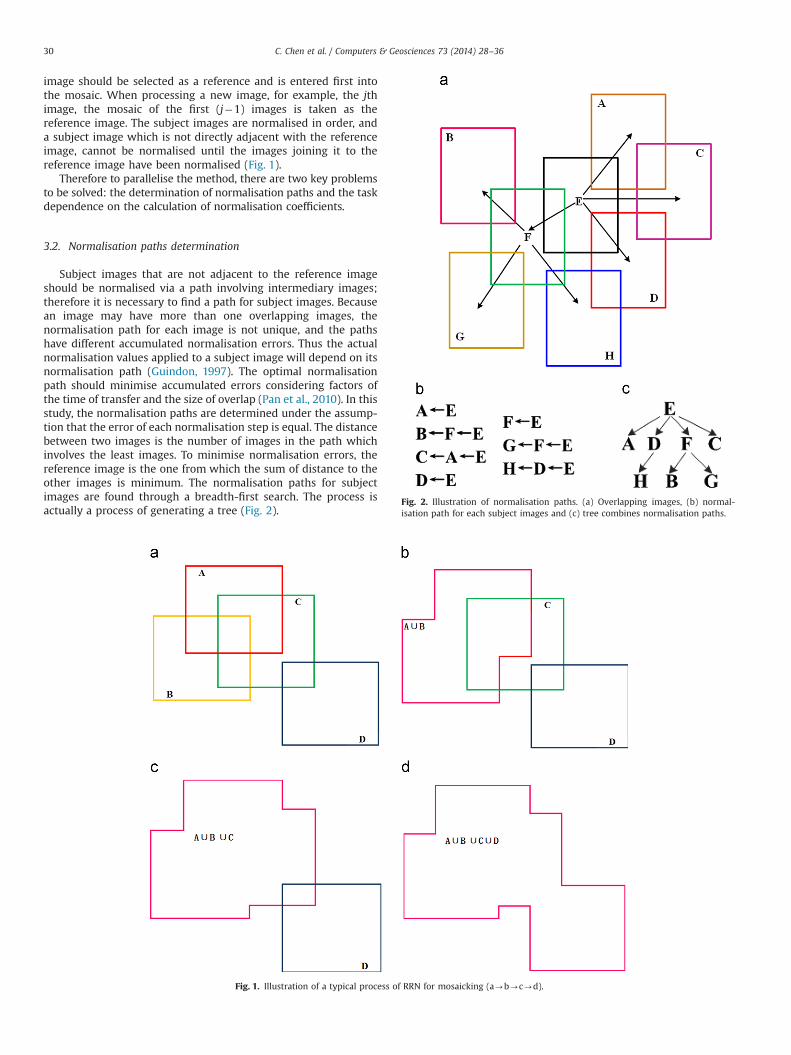
image should be selected as a reference and is entered first intothe mosaic. When processing a new image, for example, the jthimage, the mosaic of the first (j�1) images is taken as thereference image. The subject images are normalised in order, anda subject image which is not directly adjacent with the referenceimage, cannot be normalised until the images joining it to thereference image have been normalised (Fig. 1).

Therefore to parallelise the method, there are two key problemsto be solved: the determination of normalisation paths and the taskdependence on the calculation of normalisation coefficients.

3.2. Normalisation paths determination

Subject images that are not adjacent to the reference imageshould be normalised via a path involving intermediary images;therefore it is necessary to find a path for subject images. Becausean image may have more than one overlapping images, thenormalisation path for each image is not unique, and the pathshave different accumulated normalisation errors. Thus the actualnormalisation values applied to a subject image will depend on itsnormalisation path (Guindon, 1997). The optimal normalisationpath should minimise accumulated errors considering factors ofthe time of transfer and the size of overlap (Pan et al., 2010). In thisstudy, the normalisation paths are determined under the assump-tion that the error of each normalisation step is equal. The distancebetween two images is the number of images in the path whichinvolves the least images. To minimise normalisation errors, thereference image is the one from which the sum of distance to theother images is minimum. The normalisation paths for subjectimages are found through a breadth-first search. The process isactually a process of generating a tree (Fig. 2).

Fig. 1. Illustration of a typical process of RRN for mosaicking (a-b-c-d).

Fig. 2. Illustration of normalisation paths. (a) Overlapping images, (b) normal-isation path for each subject images and (c) tree combines normalisation paths.

C. Chen et al. / Computers & Geosciences 73 (2014) 28–3630

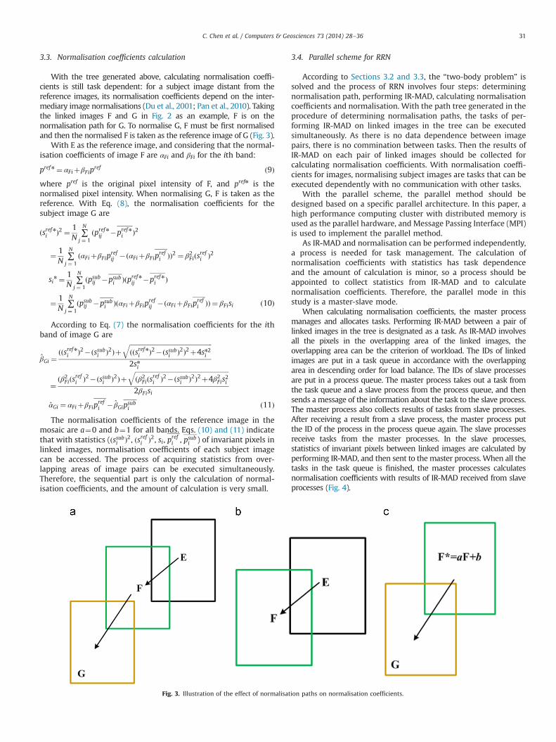
3.3. Normalisation coefficients calculation

With the tree generated above, calculating normalisation coeffi-cients is still task dependent: for a subject image distant from thereference images, its normalisation coefficients depend on the inter-mediary image normalisations (Du et al., 2001; Pan et al., 2010). Takingthe linked images F and G in Fig. 2 as an example, F is on thenormalisation path for G. To normalise G, F must be first normalisedand then the normalised F is taken as the reference image of G (Fig. 3).

With E as the reference image, and considering that the normal-isation coefficients of image F are αFi and βFi for the ith band:

prefn ¼ αFiþβFipref ð9Þ

where pref is the original pixel intensity of F, and prefn is thenormalised pixel intensity. When normalising G, F is taken as thereference. With Eq. (8), the normalisation coefficients for thesubject image G are

ðsrefni Þ2 ¼ 1N

∑N

j ¼ 1ðprefnij �prefni Þ2

¼ 1N

∑N

j ¼ 1ðαFiþβFip

refij �ðαFiþβFip

refi ÞÞ2 ¼ β2Fiðsrefi Þ2

sin ¼1N

∑N

j ¼ 1ðpsubij �psubi Þðprefnij �prefni Þ

¼ 1N

∑N

j ¼ 1ðpsubij �psubi ÞðαFiþβFip

refij �ðαFiþβFip

refi ÞÞ ¼ βFisi ð10Þ

According to Eq. (7) the normalisation coefficients for the ithband of image G are

β̂Gi ¼ððsrefni Þ2�ðssubi Þ2Þþ

ffiffiffiffiffiffiffiffiffiffiffiffiffiffiffiffiffiffiffiffiffiffiffiffiffiffiffiffiffiffiffiffiffiffiffiffiffiffiffiffiffiffiffiffiffiffiffiffiffiffiffiððsrefni Þ2�ðssubi Þ2Þ2þ4sn2i

q2sni

¼ðβ2Fiðsrefi Þ2�ðssubi Þ2Þþ

ffiffiffiffiffiffiffiffiffiffiffiffiffiffiffiffiffiffiffiffiffiffiffiffiffiffiffiffiffiffiffiffiffiffiffiffiffiffiffiffiffiffiffiffiffiffiffiffiffiffiffiffiffiffiffiffiffiffiðβ2Fiðsrefi Þ2�ðssubi Þ2Þ2þ4β2Fis

2i

q2βFisi

α̂Gi ¼ αFiþβFiprefi � β̂Gipsubi ð11Þ

The normalisation coefficients of the reference image in themosaic are a¼0 and b¼1 for all bands. Eqs. (10) and (11) indicatethat with statistics (ðssubi Þ2, ðsrefi Þ2, si, prefi , psubi ) of invariant pixels inlinked images, normalisation coefficients of each subject imagecan be accessed. The process of acquiring statistics from over-lapping areas of image pairs can be executed simultaneously.Therefore, the sequential part is only the calculation of normal-isation coefficients, and the amount of calculation is very small.

3.4. Parallel scheme for RRN

According to Sections 3.2 and 3.3, the “two-body problem” issolved and the process of RRN involves four steps: determiningnormalisation path, performing IR-MAD, calculating normalisationcoefficients and normalisation. With the path tree generated in theprocedure of determining normalisation paths, the tasks of per-forming IR-MAD on linked images in the tree can be executedsimultaneously. As there is no data dependence between imagepairs, there is no commination between tasks. Then the results ofIR-MAD on each pair of linked images should be collected forcalculating normalisation coefficients. With normalisation coeffi-cients for images, normalising subject images are tasks that can beexecuted dependently with no communication with other tasks.

With the parallel scheme, the parallel method should bedesigned based on a specific parallel architecture. In this paper, ahigh performance computing cluster with distributed memory isused as the parallel hardware, and Message Passing Interface (MPI)is used to implement the parallel method.

As IR-MAD and normalisation can be performed independently,a process is needed for task management. The calculation ofnormalisation coefficients with statistics has task dependenceand the amount of calculation is minor, so a process should beappointed to collect statistics from IR-MAD and to calculatenormalisation coefficients. Therefore, the parallel mode in thisstudy is a master-slave mode.

When calculating normalisation coefficients, the master processmanages and allocates tasks. Performing IR-MAD between a pair oflinked images in the tree is designated as a task. As IR-MAD involvesall the pixels in the overlapping area of the linked images, theoverlapping area can be the criterion of workload. The IDs of linkedimages are put in a task queue in accordance with the overlappingarea in descending order for load balance. The IDs of slave processesare put in a process queue. The master process takes out a task fromthe task queue and a slave process from the process queue, and thensends a message of the information about the task to the slave process.The master process also collects results of tasks from slave processes.After receiving a result from a slave process, the master process putthe ID of the process in the process queue again. The slave processesreceive tasks from the master processes. In the slave processes,statistics of invariant pixels between linked images are calculated byperforming IR-MAD, and then sent to the master process. When all thetasks in the task queue is finished, the master processes calculatesnormalisation coefficients with results of IR-MAD received from slaveprocesses (Fig. 4).

Fig. 3. Illustration of the effect of normalisation paths on normalisation coefficients.

C. Chen et al. / Computers & Geosciences 73 (2014) 28–36 31

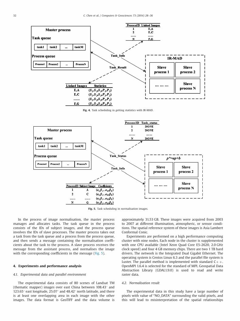
In the process of image normalisation, the master processmanages and allocates tasks. The task queue in the processconsists of the IDs of subject images, and the process queueinvolves the IDs of slave processes. The master process takes outa task from the task queue and a process from the process queue,and then sends a message containing the normalisation coeffi-cients about the task to the process. A slave process receives themessage from the assistant process, and normalises the imagewith the corresponding coefficients in the message (Fig. 5).

4. Experiments and performance analysis

4.1. Experimental data and parallel environment

The experimental data consists of 80 scenes of Landsat TM(thematic mapper) images over east China between 108.431 and123.651 east longitude, 25.071 and 48.421 north latitude, and thereis at least one overlapping area in each image with the otherimages. The data format is GeoTIFF and the data volume is

approximately 31.53 GB. These images were acquired from 2003to 2007 at different illumination, atmospheric, or sensor condi-tions. The spatial reference system of these images is Asia LambertConformal Conic.

Experiments are performed on a high performance computingcluster with nine nodes. Each node in the cluster is supplementedwith one CPU available (Intel Xeon Quad Core E5-2620, 2.0 GHzclock speed) and four 4 GB memory chips. There are two 1 TB harddrivers. The network is the Integrated Dual Gigabit Ethernet. Theoperating system is Centos Linux 6.3 and the parallel file system isLuster. The parallel method is implemented with standard Cþþ .OpenMPI 1.6.4 is selected for the standard of MPI. Geospatial DataAbstraction Library (GDAL1.9.0) is used to read and writeraster data.

4.2. Normalisation result

The experimental data in this study have a large number ofpixels with value of “NO_DATA” surrounding the valid pixels, andthis will lead to misinterpretation of the spatial relationships

Fig. 4. Task scheduling in getting statistics with IR-MAD.

Fig. 5. Task scheduling in normalisation images.

C. Chen et al. / Computers & Geosciences 73 (2014) 28–3632

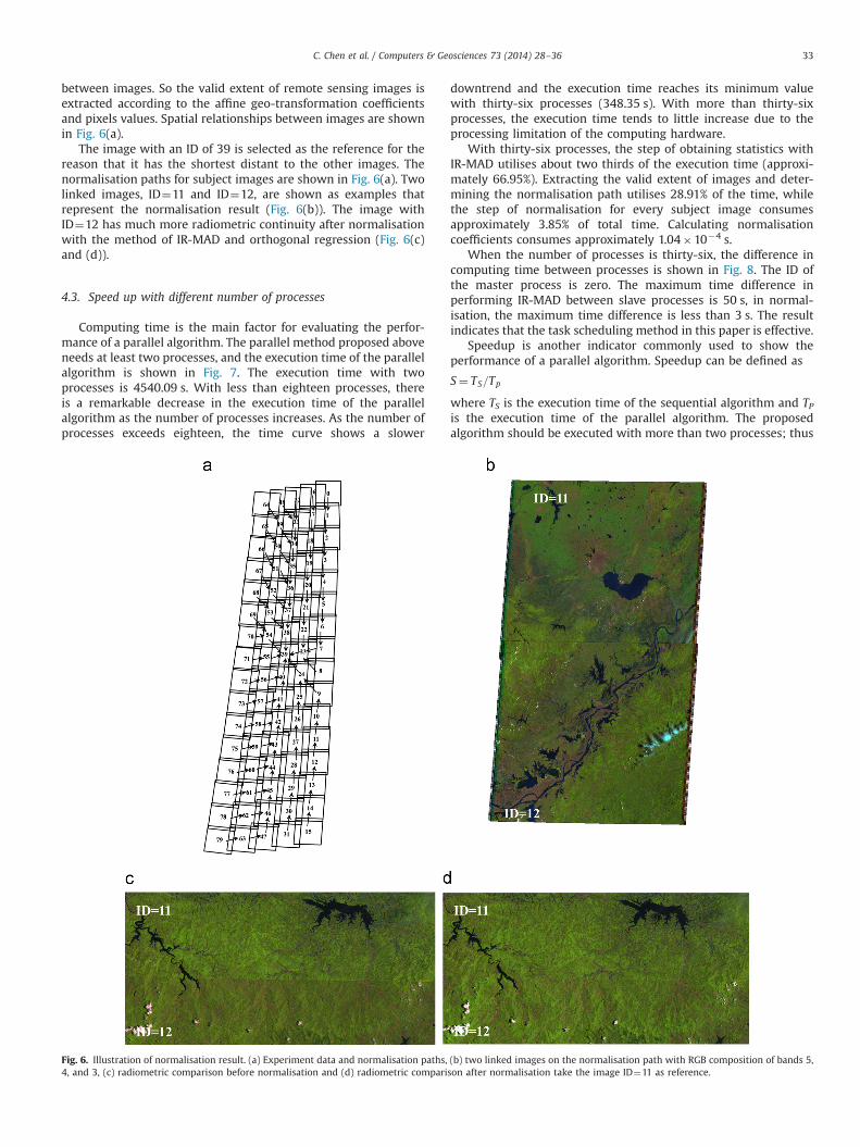
between images. So the valid extent of remote sensing images isextracted according to the affine geo-transformation coefficientsand pixels values. Spatial relationships between images are shownin Fig. 6(a).

The image with an ID of 39 is selected as the reference for thereason that it has the shortest distant to the other images. Thenormalisation paths for subject images are shown in Fig. 6(a). Twolinked images, ID¼11 and ID¼12, are shown as examples thatrepresent the normalisation result (Fig. 6(b)). The image withID¼12 has much more radiometric continuity after normalisationwith the method of IR-MAD and orthogonal regression (Fig. 6(c)and (d)).

4.3. Speed up with different number of processes

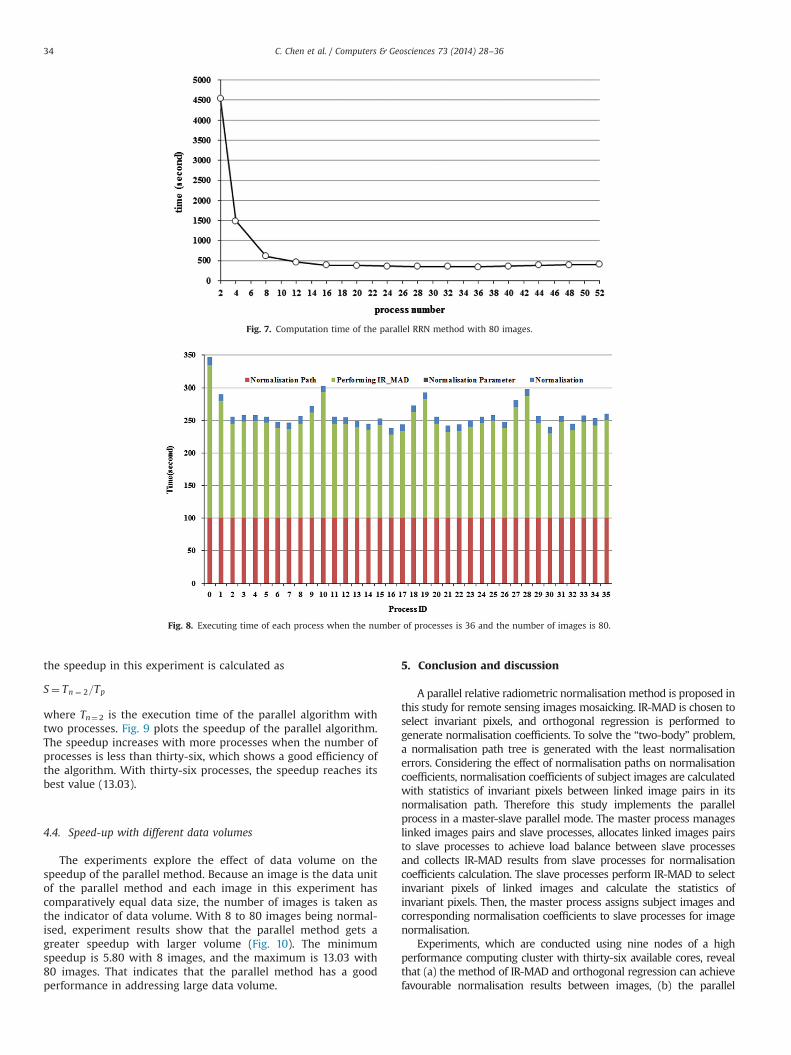
Computing time is the main factor for evaluating the perfor-mance of a parallel algorithm. The parallel method proposed aboveneeds at least two processes, and the execution time of the parallelalgorithm is shown in Fig. 7. The execution time with twoprocesses is 4540.09 s. With less than eighteen processes, thereis a remarkable decrease in the execution time of the parallelalgorithm as the number of processes increases. As the number ofprocesses exceeds eighteen, the time curve shows a slower

downtrend and the execution time reaches its minimum valuewith thirty-six processes (348.35 s). With more than thirty-sixprocesses, the execution time tends to little increase due to theprocessing limitation of the computing hardware.

With thirty-six processes, the step of obtaining statistics withIR-MAD utilises about two thirds of the execution time (approxi-mately 66.95%). Extracting the valid extent of images and deter-mining the normalisation path utilises 28.91% of the time, whilethe step of normalisation for every subject image consumesapproximately 3.85% of total time. Calculating normalisationcoefficients consumes approximately 1.04�10�4 s.

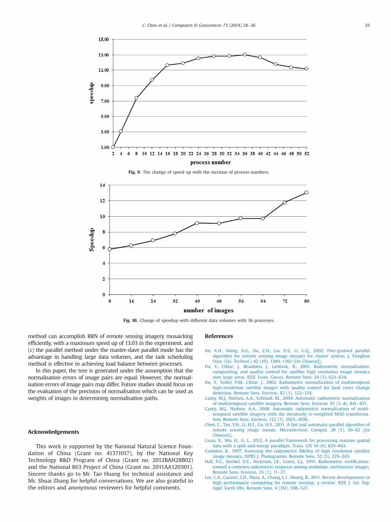
When the number of processes is thirty-six, the difference incomputing time between processes is shown in Fig. 8. The ID ofthe master process is zero. The maximum time difference inperforming IR-MAD between slave processes is 50 s, in normal-isation, the maximum time difference is less than 3 s. The resultindicates that the task scheduling method in this paper is effective.

Speedup is another indicator commonly used to show theperformance of a parallel algorithm. Speedup can be defined as

S¼ TS=Tp

where TS is the execution time of the sequential algorithm and TPis the execution time of the parallel algorithm. The proposedalgorithm should be executed with more than two processes; thus

Fig. 6. Illustration of normalisation result. (a) Experiment data and normalisation paths, (b) two linked images on the normalisation path with RGB composition of bands 5,4, and 3, (c) radiometric comparison before normalisation and (d) radiometric comparison after normalisation take the image ID¼11 as reference.

C. Chen et al. / Computers & Geosciences 73 (2014) 28–36 33

the speedup in this experiment is calculated as

S¼ Tn ¼ 2=Tp

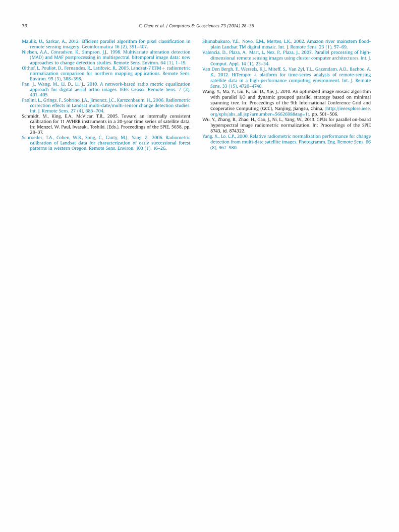
where Tn¼2 is the execution time of the parallel algorithm withtwo processes. Fig. 9 plots the speedup of the parallel algorithm.The speedup increases with more processes when the number ofprocesses is less than thirty-six, which shows a good efficiency ofthe algorithm. With thirty-six processes, the speedup reaches itsbest value (13.03).

4.4. Speed-up with different data volumes

The experiments explore the effect of data volume on thespeedup of the parallel method. Because an image is the data unitof the parallel method and each image in this experiment hascomparatively equal data size, the number of images is taken asthe indicator of data volume. With 8 to 80 images being normal-ised, experiment results show that the parallel method gets agreater speedup with larger volume (Fig. 10). The minimumspeedup is 5.80 with 8 images, and the maximum is 13.03 with80 images. That indicates that the parallel method has a goodperformance in addressing large data volume.

5. Conclusion and discussion

A parallel relative radiometric normalisation method is proposed inthis study for remote sensing images mosaicking. IR-MAD is chosen toselect invariant pixels, and orthogonal regression is performed togenerate normalisation coefficients. To solve the “two-body” problem,a normalisation path tree is generated with the least normalisationerrors. Considering the effect of normalisation paths on normalisationcoefficients, normalisation coefficients of subject images are calculatedwith statistics of invariant pixels between linked image pairs in itsnormalisation path. Therefore this study implements the parallelprocess in a master-slave parallel mode. The master process manageslinked images pairs and slave processes, allocates linked images pairsto slave processes to achieve load balance between slave processesand collects IR-MAD results from slave processes for normalisationcoefficients calculation. The slave processes perform IR-MAD to selectinvariant pixels of linked images and calculate the statistics ofinvariant pixels. Then, the master process assigns subject images andcorresponding normalisation coefficients to slave processes for imagenormalisation.

Experiments, which are conducted using nine nodes of a highperformance computing cluster with thirty-six available cores, revealthat (a) the method of IR-MAD and orthogonal regression can achievefavourable normalisation results between images, (b) the parallel

Fig. 7. Computation time of the parallel RRN method with 80 images.

Fig. 8. Executing time of each process when the number of processes is 36 and the number of images is 80.

C. Chen et al. / Computers & Geosciences 73 (2014) 28–3634

method can accomplish RRN of remote sensing imagery mosaickingefficiently, with a maximum speed up of 13.03 in the experiment, and(c) the parallel method under the master-slave parallel mode has theadvantage in handling large data volumes, and the task schedulingmethod is effective in achieving load balance between processes.

In this paper, the tree is generated under the assumption that thenormalisation errors of image pairs are equal. However, the normal-isation errors of image pairs may differ. Future studies should focus onthe evaluation of the precision of normalisation which can be used asweights of images in determining normalisation paths.

Acknowledgements

This work is supported by the National Natural Science Foun-dation of China (Grant no. 41371017), by the National KeyTechnology R&D Program of China (Grant no. 2012BAH28B02)and the National 863 Project of China (Grant no. 2011AA120301).Sincere thanks go to Mr. Tao Huang for technical assistance andMr. Shuai Zhang for helpful conversations. We are also grateful tothe editors and anonymous reviewers for helpful comments.

References

An, X.H., Wang, X.G., Du, Z.H., Liu, D.S., Li, G.Q., 2002. Fine-grained parallelalgorithm for remote sensing image mosaics for cluster system. J. TsinghuaUniv. (Sci. Technol.) 42 (10), 1389–1392 ([in Chinese]).

Du, Y., Cihlar, J., Beaubien, J., Latifovic, R., 2001. Radiometric normalization,compositing, and quality control for satellite high resolution image mosaicsover large areas. IEEE Trans. Geosci. Remote Sens. 39 (3), 623–634.

Du, Y., Teillet, P.M., Cihlar, J., 2002. Radiometric normalization of multitemporalhigh-resolution satellite images with quality control for land cover changedetection. Remote Sens. Environ. 82 (1), 123–134.

Canty, M.J., Nielsen, A.A., Schmidt, M., 2004. Automatic radiometric normalizationof multitemporal satellite imagery. Remote Sens. Environ. 91 (3–4), 441–451.

Canty, M.J., Nielsen, A.A., 2008. Automatic radiometric normalization of multi-temporal satellite imagery with the iteratively re-weighted MAD transforma-tion. Remote Sens. Environ. 112 (3), 1025–1036.

Chen, C., Tan, Y.H., Li, H.T., Gu, H.Y., 2011. A fast and automatic parallel algorithm ofremote sensing image mosaic. Microelectron. Comput. 28 (3), 59–62 ([inChinese]).

Guan, X., Wu, H., Li, L., 2012. A parallel framework for processing massive spatialdata with a split-and-merge paradigm. Trans. GIS 16 (6), 829–843.

Guindon, B., 1997. Assessing the radiometric fidelity of high resolution satelliteimage mosaics. ISPRS J. Photogramm. Remote Sens. 52 (5), 229–243.

Hall, F.G., Strebel, D.E., Nickeson, J.E., Goetz, S.J., 1991. Radiometric rectification:toward a common radiometric response among multidate, multisensor images.Remote Sens. Environ. 35 (1), 11–27.

Lee, C.A., Gasster, S.D., Plaza, A., Chang, C.I., Huang, B., 2011. Recent developments inhigh performance computing for remote sensing: a review. IEEE J. Sel. Top.Appl. Earth Obs. Remote Sens. 4 (3SI), 508–527.

Fig. 9. The change of speed up with the increase of process numbers.

Fig. 10. Change of speedup with different data volumes with 36 processes.

C. Chen et al. / Computers & Geosciences 73 (2014) 28–36 35

Maulik, U., Sarkar, A., 2012. Efficient parallel algorithm for pixel classification inremote sensing imagery. Geoinformatica 16 (2), 391–407.

Nielsen, A.A., Conradsen, K., Simpson, J.J., 1998. Multivariate alteration detection(MAD) and MAF postprocessing in multispectral, bitemporal image data: newapproaches to change detection studies. Remote Sens. Environ. 64 (1), 1–19.

Olthof, I., Pouliot, D., Fernandes, R., Latifovic, R., 2005. Landsat-7 ETMþ radiometricnormalization comparison for northern mapping applications. Remote Sens.Environ. 95 (3), 388–398.

Pan, J., Wang, M., Li, D., Li, J., 2010. A network-based radio metric equalizationapproach for digital aerial ortho images. IEEE Geosci. Remote Sens. 7 (2),401–405.

Paolini, L., Grings, F., Sobrino, J.A., Jimenez, J.C., Karszenbaum, H., 2006. Radiometriccorrection effects in Landsat multi-date/multi-sensor change detection studies.Int. J. Remote Sens. 27 (4), 685–704.

Schmidt, M., King, E.A., McVicar, T.R., 2005. Toward an internally consistentcalibration for 11 AVHRR instruments in a 20-year time series of satellite data.In: Menzel, W. Paul, Iwasaki, Toshiki. (Eds.), Proceedings of the SPIE, 5658, pp.28–37.

Schroeder, T.A., Cohen, W.B., Song, C., Canty, M.J., Yang, Z., 2006. Radiometriccalibration of Landsat data for characterization of early successional forestpatterns in western Oregon. Remote Sens. Environ. 103 (1), 16–26.

Shimabukuro, Y.E., Novo, E.M., Mertes, L.K., 2002. Amazon river mainstem flood-plain Landsat TM digital mosaic. Int. J. Remote Sens. 23 (1), 57–69.

Valencia, D., Plaza, A., Mart, I., Nez, P., Plaza, J., 2007. Parallel processing of high-dimensional remote sensing images using cluster computer architectures. Int. J.Comput. Appl. 14 (1), 23–34.

Van Den Bergh, F., Wessels, K.J., Miteff, S., Van Zyl, T.L., Gazendam, A.D., Bachoo, A.K., 2012. HiTempo: a platform for time-series analysis of remote-sensingsatellite data in a high-performance computing environment. Int. J. RemoteSens. 33 (15), 4720–4740.

Wang, Y., Ma, Y., Liu, P., Liu, D., Xie, J., 2010. An optimized image mosaic algorithmwith parallel I/O and dynamic grouped parallel strategy based on minimalspanning tree. In: Proceedings of the 9th International Conference Grid andCooperative Computing (GCC), Nanjing, Jiangsu, China, ⟨http://ieeexplore.ieee.org/xpls/abs_all.jsp?arnumber=5662698&tag=1⟩. pp. 501–506.

Wu, Y., Zhang, B., Zhao, H., Gao, J., Ni, L., Yang, W., 2013. GPUs for parallel on-boardhyperspectral image radiometric normalization. In: Proceedings of the SPIE8743, id. 874322.

Yang, X., Lo, C.P., 2000. Relative radiometric normalization performance for changedetection from multi-date satellite images. Photogramm. Eng. Remote Sens. 66(8), 967–980.

C. Chen et al. / Computers & Geosciences 73 (2014) 28–3636