parallel quicksort algorithms with isoefﬁciency analysis€¦ · parallel quicksort...

Parallel quicksort algorithmswith isoefficiency analysis

Parallel quicksort algorithmswith isoefficiency analysis – p. 1

Overview

Sequential quicksort algorithm

Three parallel quicksort algorithms

Isoefficiency analysis

Chapter 14 and Chapter 7.6 in Michael J. Quinn, Parallel Programmingin C with MPI and OpenMP


Quicksort

Given a list of numbers, we want to sort the numbers in an increasingorder

The same as finding a suitable permutation

Sequential quicksort algorithm: a recursive procedureSelect one of the numbers as pivotDivide the list into two sublists: a “low list” containing numberssmaller than the pivot, and a “high list” containing numbers largerthan the pivotThe low list and high list recursively repeat the procedure to sortthemselvesThe final sorted result is the concatenation of the sorted low list,the pivot, and the sorted high list


Example of quicksort

Given a list of numbers: {79, 17, 14, 65, 89, 4, 95, 22, 63, 11}

The first number, 79, is chosen as pivotLow list contains {17, 14, 65, 4, 22, 63, 11}

High list contains {89, 95}

For sublist {17, 14, 65, 4, 22, 63, 11}, choose 17 as pivot

Low list contains {14, 4, 11}

High list contains {64, 22, 63}

. . .

{4, 11, 14, 17, 22, 63, 65} is the sorted result of sublist{17, 14, 65, 4, 22, 63, 11}

For sublist {89, 95} choose 89 as pivotLow list is empty (no need for further recursions)High list contains {95} (no need for further recursions)

{89, 95} is the sorted result of sublist {89, 95}

Final sorted result: {4, 11, 14, 17, 22, 63, 65, 79, 89, 95}Parallel quicksort algorithmswith isoefficiency analysis – p. 4

Illustration of quicksort

Figure 14.1 from Parallel Programming in C with MPI and OpenMP


Two observartions

Quicksort is generally recognized, in the average case, as the fastestsorting algorithm

Quicksort has some natural concurrencyThe low list and high list can sort themselves concurrently


Parallelizing quicksort

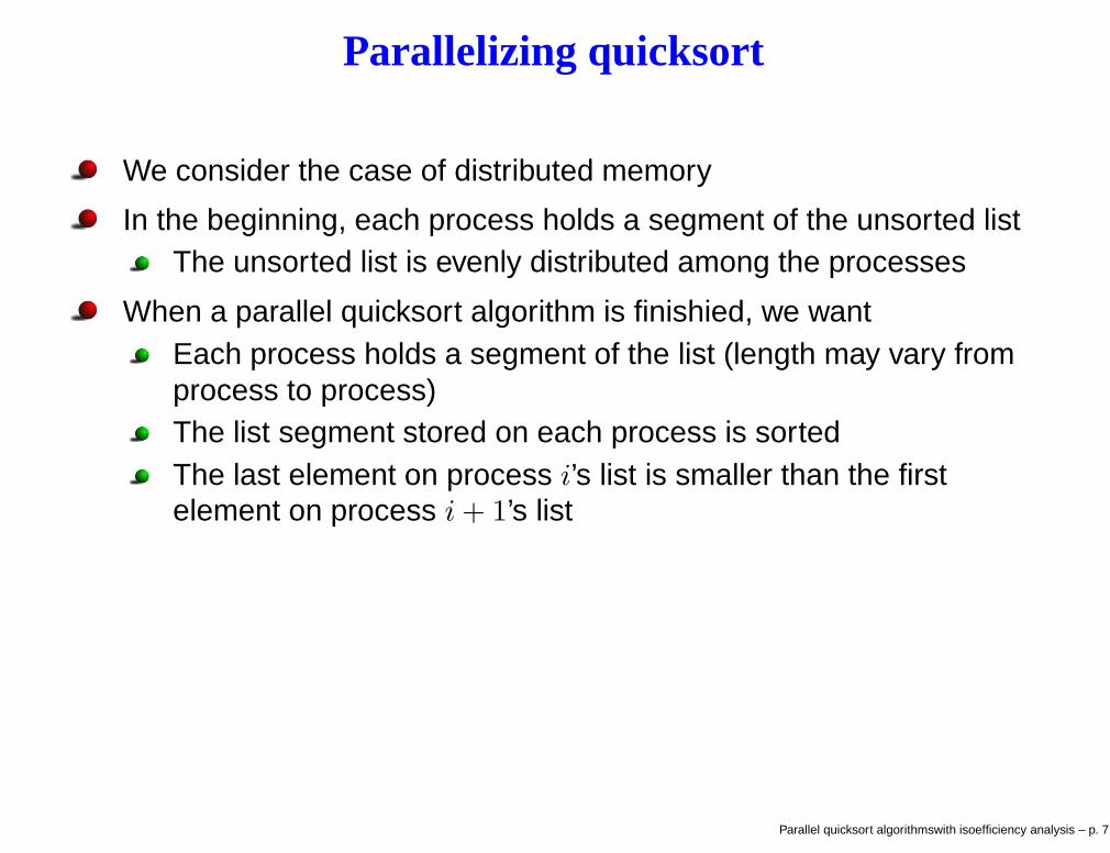
We consider the case of distributed memory

In the beginning, each process holds a segment of the unsorted listThe unsorted list is evenly distributed among the processes

When a parallel quicksort algorithm is finishied, we wantEach process holds a segment of the list (length may vary fromprocess to process)The list segment stored on each process is sortedThe last element on process i’s list is smaller than the firstelement on process i+ 1’s list


Parallel quicksort algorithm 1

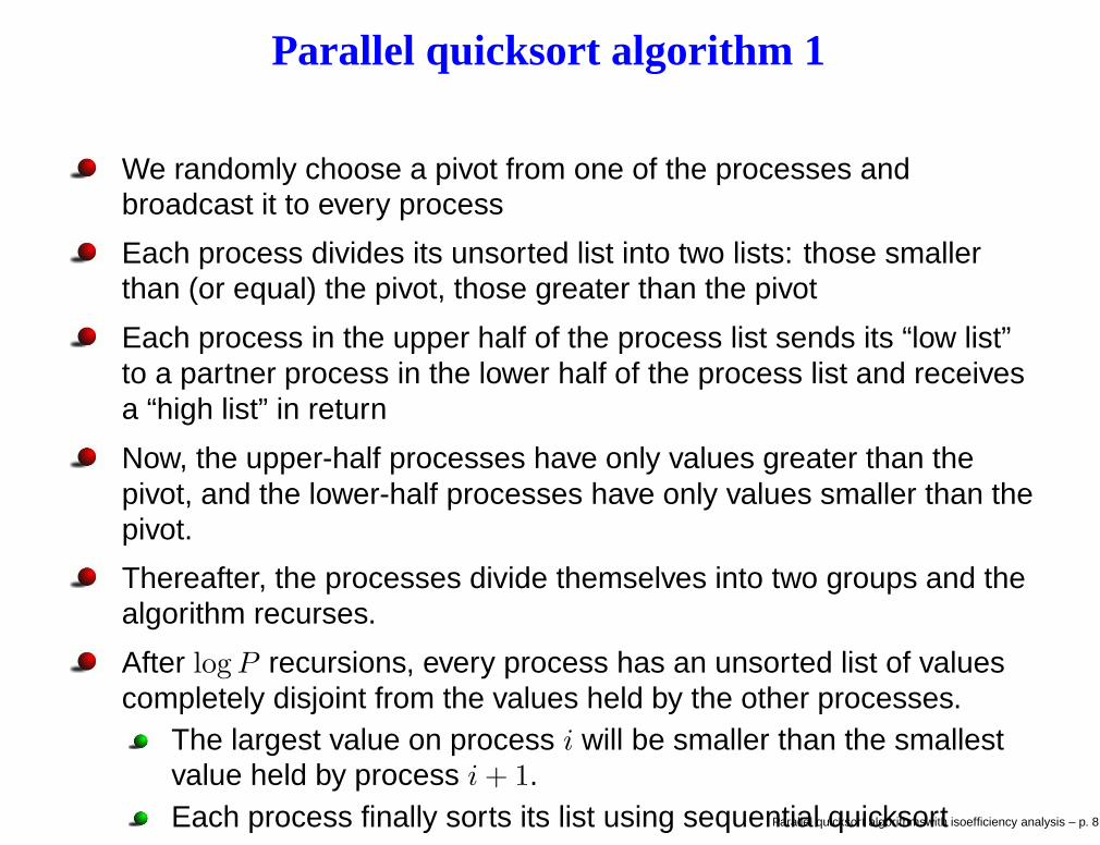
We randomly choose a pivot from one of the processes andbroadcast it to every process

Each process divides its unsorted list into two lists: those smallerthan (or equal) the pivot, those greater than the pivot

Each process in the upper half of the process list sends its “low list”to a partner process in the lower half of the process list and receivesa “high list” in return

Now, the upper-half processes have only values greater than thepivot, and the lower-half processes have only values smaller than thepivot.

Thereafter, the processes divide themselves into two groups and thealgorithm recurses.

After logP recursions, every process has an unsorted list of valuescompletely disjoint from the values held by the other processes.

The largest value on process i will be smaller than the smallestvalue held by process i+ 1.Each process finally sorts its list using sequential quicksortParallel quicksort algorithmswith isoefficiency analysis – p. 8

Illustration of parallel quicksort 1



Analysis of parallel quicksort 1

This parallel quicksort algorithm is likely to do a poor job of loadbalancing

If the pivot value is not the median value, we will not divide the listinto two equal sublistsFinding the median value is prohibitively expensive on a parallelcomputer

The remedy is to choose the pivot value close to the true median!


Hyperquicksort – parallel quicksort 2

Each process starts with a sequential quicksort on its local list

Now we have a better chance to choose a pivot that is close to thetrue median

The process that is responsible for choosing the pivot can pickthe median of its local list

The following three next steps of hyperquicksort are the same as inparallel quicksort 1

broadcastdivision of “low list” and high list”swap between partner processes

The 4th step is different from parallel quicksort 1One each process, the remaining half of local list and thereceived half-list are merged into a sorted local list

Recursion within upper-half processes and lower-half processes . . .


Example of using hyperquicksort



Some observations about hyperquicksort

logP steps are needed in the recursionThe average number of times a value is passed from one processto another is log P

2 , therefore quite some communicationoverhead!

The median value chosen from a local segment may still be quitedifferent from the true median of the entire list

Load imbalance may still arise, although better than parallelquicksort algorithm 1How good exactly is hyperquicksort?We can make use of the so-called isoefficiency relation


Isoefficiency relation

Purpose: To find the scalability of a parallel program

Definition of scalability: The ability to maintain efficiency when thenumber of processes is increased

Recall that due to the inherently sequential work and communicationoverhead, parallel efficiency of a fixed-sized problem will decreasewhen more processes (p) are used

To maintain the same level of efficiency, the problem size mustincrease together with p

Chapter 7.6 of the textbook


Isoefficiency relation (2)

Recall the definition of speedup

ψ(n, p) ≤σ(n) + ϕ(n)

σ(n) + ϕ(n)/p+ κ(n, p)

=p (σ(n) + ϕ(n))

pσ(n) + ϕ(n) + pκ(n, p)

=p (σ(n) + ϕ(n))

σ(n) + ϕ(n) + (p− 1)σ(n) + pκ(n, p)



We denote To(n, p) to be the total time spent by all processes doingwork that is above σ(n) + ϕ(n)

That is

To(n, p) = p T (n, p) − (σ(n) + ϕ(n)) = (p− 1)σ(n) + pκ(n, p)

Therefore

ψ(n, p) ≤p (σ(n) + ϕ(n))

σ(n) + ϕ(n) + To(n, p)



Recall efficiency ε(n, p) is ψ(n, p) divided by p

Therefore

ε(n, p) ≤σ(n) + ϕ(n)

σ(n) + ϕ(n) + To(n, p)

=1

1 + To(n,p)σ(n)+ϕ(n)



Recall the sequential execution time: T (n, 1) = σ(n) + ϕ(n)

That is,

ε(n, p) ≤1

1 + To(n,p)T (n,1)

Therefore, we can derive

To(n, p)

T (n, 1)≤

1 − ε(n, p)

ε(n, p)

Consequently,

T (n, 1) ≥ε(n, p)

1 − ε(n, p)To(n, p)

In other words, if we want ε(n, p) to remain constant (when both p and

n increase), we must have T (n, 1) ≥ C To(n, p), where C = ε(n,p)1−ε(n,p)


What has isoefficiency relation told us?

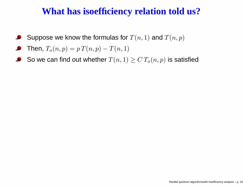
Suppose we know the formulas for T (n, 1) and T (n, p)

Then, To(n, p) = p T (n, p) − T (n, 1)

So we can find out whether T (n, 1) ≥ C To(n, p) is satisfied


Consideration of memory usage

Memory usage M(n) (as function of n) can be a limiting factor

Suppose the isoefficiency relation says n ≥ f(p)

This in fact says thatn ≥M(f(p))

Hence M(f(p))/p indicates how the memory usage per processormust increase as a function of p, in order to maintain the same levelof efficiency

We call M(f(p))/p the scalability function

For example, M(f(p))/p = O(1) means perfect scalability

However, if M(f(p))/p = O(p), the parallel efficiency can not bemaintained forever


Applying isoefficiency analysis to hyperquicksort

Assume there are n values to be sorted, using p processes, and thatn≫ p.

In the beginning, each process has ⌈n/p⌉ values

Cost of initial sequential quicksort per process: O((n/p) log(n/p))

In every split-and-merge step, each process keeps on average n/2pvalues and transmits n/2p values

Cost of communication per process: O(n/p)

There are log p iterations, so total communication cost per process:κ(n, p) = O(n log p/p) (cost of broadcast is neglected because n≫ p)

In addition, we have σ(n) = 0 (no inherently sequential work)

Therefore,

To(n, p) = (p− 1)σ(n) + pκ(n, p) = O(n log p)


More analysis of hyperquicksort

Isoefficiency relation requires T (n, 1) ≥ CTo(n, p)

We have now T (n, 1) = O(n logn) and To(n, p) = O(n log p)

Therefore, the following condition must satisfy:

n logn ≥ Cn log p ⇒ logn ≥ C log p ⇒ n ≥ pC

Memory requirement is simple: M(n) = n

Therefore the scalability function M(pC)/p = pC

p= pC−1

If C > 2, scalability is low


Algorithm 3 – parallel sorting by regular sampling

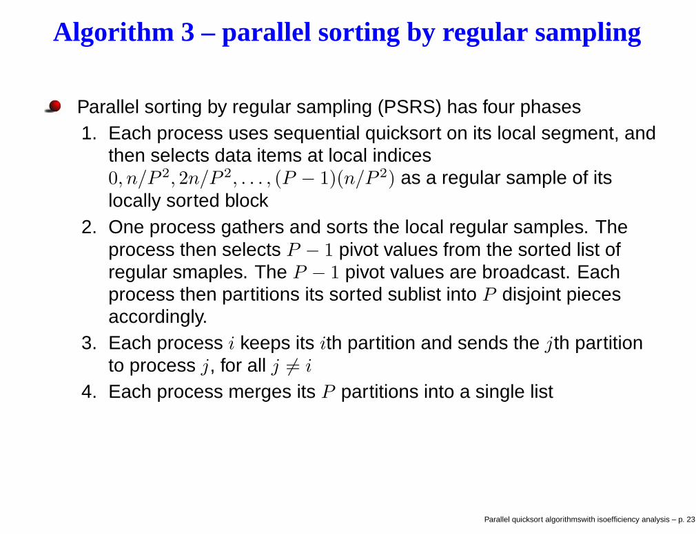
Parallel sorting by regular sampling (PSRS) has four phases1. Each process uses sequential quicksort on its local segment, and

then selects data items at local indices0, n/P 2, 2n/P 2, . . . , (P − 1)(n/P 2) as a regular sample of itslocally sorted block

2. One process gathers and sorts the local regular samples. Theprocess then selects P − 1 pivot values from the sorted list ofregular smaples. The P − 1 pivot values are broadcast. Eachprocess then partitions its sorted sublist into P disjoint piecesaccordingly.

3. Each process i keeps its ith partition and sends the jth partitionto process j, for all j 6= i

4. Each process merges its P partitions into a single list


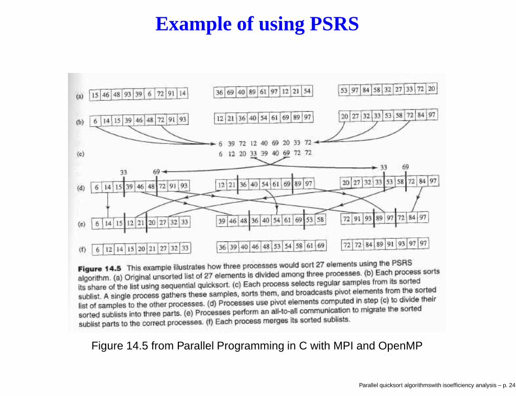
Example of using PSRS



Three advantages of PSRS

1. Better load balance (although perfect load balance can not beguaranteed)

2. Repeated communications of a same value are avoided

3. The number of processes does not have to be power of 2, which isrequired by parallel quicksort algorithm 1 and hyperquicksort

Additional comment: The isoefficiency analysis of PSRS is similar tohyperquicksort


parallel quicksort algorithms with isoefﬁciency analysis€¦ · parallel quicksort...

Documents