parallel intrusion detection systems for high speed

PARALLEL INTRUSION DETECTION SYSTEMS FOR HIGHSPEED NETWORKS USING THE DIVIDED DATA PARALLEL

METHOD

By

Christopher Vincent Kopek

A Thesis Submitted to the Graduate Faculty of

WAKE FOREST UNIVERSITY

in Partial Fulfillment of the Requirements

for the Degree of

MASTER OF SCIENCE

in the Department of Computer Science

May, 2007

Winston-Salem, North Carolina

Approved By:

Errin W. Fulp, Ph.D., Advisor

Examining Committee:

Stan Thomas, Ph.D., Chairperson

William Turkett, Ph.D.

Acknowledgements

My time at Wake Forest University has been limited, but in that time I was ableto form many lasting relationships. I first want to thank all my friends for supportingme and helping me enjoy my time at Wake. Without the crazy lab adventures, mymemories would not be the same. I personally want to thank Michael Horvath forkeeping me company in the networking lab and destroying me in lab basketball andbaseball. I want to thank my family for supporting me throughout my graduateschool career. They encouraged me to always do my best and strive to be better.

This thesis would not be the same if it were not for my committee helping mealong the way. Their constant help and notes of advice, not only helped me with mythesis, but helped me learn how to become a better technical writer. In particular Iwant to thank Dr. Fulp, my advisor. Our near daily meetings helped me mold myideas into a solid thesis, become a better computer scientist, and keep my mind saneat the same time.

I want to thank GreatWall Systems, Inc. for providing me the equipment to workon, and the employment opportunities. By working on the equipment, I was able toproduce quality results, and by interning, I was able to work on my creative researchabilities. Finally, I want to thank anyone else who I did not explicitly mention for allyour support.

ii

Table of Contents

Acknowledgements . . . . . . . . . . . . . . . . . . . . . . . . . . . . . . . . . . . . . . . . . . . . . . . . . . ii

Illustrations . . . . . . . . . . . . . . . . . . . . . . . . . . . . . . . . . . . . . . . . . . . . . . . . . . . . . . . . . vi

Abbreviations . . . . . . . . . . . . . . . . . . . . . . . . . . . . . . . . . . . . . . . . . . . . . . . . . . . . . . . viii

Abstract . . . . . . . . . . . . . . . . . . . . . . . . . . . . . . . . . . . . . . . . . . . . . . . . . . . . . . . . . . . . ix

Chapter 1 Introduction . . . . . . . . . . . . . . . . . . . . . . . . . . . . . . . . . . . . . . . . . . . . 1

1.1 Intrusion Detection System Overview . . . . . . . . . . . . . . . . . . 1

1.2 Snort an Open-Source IDS . . . . . . . . . . . . . . . . . . . . . . . . 3

1.3 High Speed IDS . . . . . . . . . . . . . . . . . . . . . . . . . . . . . . 5

1.4 Outline . . . . . . . . . . . . . . . . . . . . . . . . . . . . . . . . . . . 5

Chapter 2 Analysis of Snort Content Matching . . . . . . . . . . . . . . . . . . . . 6

2.1 Dissection of Content Matching Rules . . . . . . . . . . . . . . . . . . 6

2.1.1 Rule Header . . . . . . . . . . . . . . . . . . . . . . . . . . . . 7

2.1.2 Rule Options . . . . . . . . . . . . . . . . . . . . . . . . . . . 9

2.2 Snort Content Matching Process . . . . . . . . . . . . . . . . . . . . . 11

Chapter 3 Snort Content Matching Algorithms . . . . . . . . . . . . . . . . . . . . 12

3.1 Boyer-Moore Algorithm . . . . . . . . . . . . . . . . . . . . . . . . . 12

3.2 Wu-Manber Algorithm . . . . . . . . . . . . . . . . . . . . . . . . . . 15

3.2.1 Preprocessing Stage . . . . . . . . . . . . . . . . . . . . . . . . 15

3.2.2 Searching Stage . . . . . . . . . . . . . . . . . . . . . . . . . . 17

3.2.3 Modified Wu-Manber . . . . . . . . . . . . . . . . . . . . . . . 19

3.3 Aho-Corasick Algorithm . . . . . . . . . . . . . . . . . . . . . . . . . 20

3.3.1 Goto Function . . . . . . . . . . . . . . . . . . . . . . . . . . . 20

3.3.2 Failure Function . . . . . . . . . . . . . . . . . . . . . . . . . 22

3.3.3 Output Function . . . . . . . . . . . . . . . . . . . . . . . . . 23

3.4 Alternative Content Matching Algorithms . . . . . . . . . . . . . . . 24

3.4.1 Dual-Algorithm . . . . . . . . . . . . . . . . . . . . . . . . . . 24

3.4.2 Piranha . . . . . . . . . . . . . . . . . . . . . . . . . . . . . . 25

3.4.3 E2xb . . . . . . . . . . . . . . . . . . . . . . . . . . . . . . . . 26

iii

iv

Chapter 4 Parallel Content Matching . . . . . . . . . . . . . . . . . . . . . . . . . . . . . . 27

4.1 Content Matching Parallelism . . . . . . . . . . . . . . . . . . . . . . 28

4.2 Function Parallel . . . . . . . . . . . . . . . . . . . . . . . . . . . . . 28

4.3 Data Parallel . . . . . . . . . . . . . . . . . . . . . . . . . . . . . . . 30

4.3.1 Traditional Data Parallel using Wu-Manber . . . . . . . . . . 30

4.3.2 Data Parallel Dual-Algorithm using Wu-Manber . . . . . . . . 30

4.3.3 Data Parallel using Packet Division . . . . . . . . . . . . . . . 31

Chapter 5 Divided Data Parallel Method . . . . . . . . . . . . . . . . . . . . . . . . . . 35

5.1 False Negative Avoidance . . . . . . . . . . . . . . . . . . . . . . . . 35

5.2 Synchronization Array . . . . . . . . . . . . . . . . . . . . . . . . . . 37

5.3 Design of the DDP Method . . . . . . . . . . . . . . . . . . . . . . . 39

5.4 Aho-Corasick and Wu-Manber Content Matching Algorithms . . . . . 41

Chapter 6 Experimental Evaluation of Parallel Techniques . . . . . . . . . 43

6.1 System Design . . . . . . . . . . . . . . . . . . . . . . . . . . . . . . . 43

6.1.1 Linux System . . . . . . . . . . . . . . . . . . . . . . . . . . . 44

6.1.2 Default and Expert Rule Set . . . . . . . . . . . . . . . . . . . 44

6.1.3 Experiment Construction . . . . . . . . . . . . . . . . . . . . . 45

6.2 Current Parallel Approaches . . . . . . . . . . . . . . . . . . . . . . . 47

6.2.1 Data Parallel Extended with Aho-Corasick . . . . . . . . . . . 47

6.2.2 Data Parallel using Snort Wu-Manber . . . . . . . . . . . . . 49

6.2.3 Data Parallel using Dual-Algorithm . . . . . . . . . . . . . . . 50

6.2.4 Function Parallel using Wu-Manber . . . . . . . . . . . . . . . 52

6.3 Divided Data Parallel Method . . . . . . . . . . . . . . . . . . . . . . 54

6.3.1 Effect of Overlap . . . . . . . . . . . . . . . . . . . . . . . . . 55

6.3.2 Effect of Synchronization . . . . . . . . . . . . . . . . . . . . . 56

6.3.3 DDP Results . . . . . . . . . . . . . . . . . . . . . . . . . . . 56

6.4 Wu-Manber with Excludes . . . . . . . . . . . . . . . . . . . . . . . . 60

6.5 Outstanding Issues . . . . . . . . . . . . . . . . . . . . . . . . . . . . 61

Chapter 7 Conclusions and Future Work . . . . . . . . . . . . . . . . . . . . . . . . . . . 66

References . . . . . . . . . . . . . . . . . . . . . . . . . . . . . . . . . . . . . . . . . . . . . . . . . . . . . . . . . . 69

Appendix A Expert Rule Set Timings . . . . . . . . . . . . . . . . . . . . . . . . . . . . . . 72

Appendix B Snort Rule Set Timings . . . . . . . . . . . . . . . . . . . . . . . . . . . . . . . 74

Appendix C DDP Rule Set Variations. . . . . . . . . . . . . . . . . . . . . . . . . . . . . . 76

v

Appendix D Other Timings . . . . . . . . . . . . . . . . . . . . . . . . . . . . . . . . . . . . . . . . 78

D.1 Function Parallel . . . . . . . . . . . . . . . . . . . . . . . . . . . . . 78

D.2 Wu-Manber Excludes . . . . . . . . . . . . . . . . . . . . . . . . . . . 78

Vita . . . . . . . . . . . . . . . . . . . . . . . . . . . . . . . . . . . . . . . . . . . . . . . . . . . . . . . . . . . . . . . . . 80

Illustrations

List of Tables

A.1 Trace 1 times in milliseconds . . . . . . . . . . . . . . . . . . . . . . . 72






B.1 Trace 1 times in milliseconds . . . . . . . . . . . . . . . . . . . . . . . 74






C.1 Trace 1 times in milliseconds . . . . . . . . . . . . . . . . . . . . . . . 76






D.1 Time for traces in milliseconds . . . . . . . . . . . . . . . . . . . . . . 78

D.2 Trace 1 times in milliseconds . . . . . . . . . . . . . . . . . . . . . . . 78






List of Figures

1.1 Intrusion Detection System Type State Diagrams . . . . . . . . . . . 3

vi

vii

2.1 The two main sections of a Snort rule . . . . . . . . . . . . . . . . . . 6

2.2 Snort rule header . . . . . . . . . . . . . . . . . . . . . . . . . . . . . 7

2.3 Snort rule with content option . . . . . . . . . . . . . . . . . . . . . . 9

2.4 Snort rule with content and options . . . . . . . . . . . . . . . . . . . 9

3.1 Aho-Corasick Functions . . . . . . . . . . . . . . . . . . . . . . . . . 22

4.1 Data parallel system using packet division . . . . . . . . . . . . . . . 32

4.2 Packet overlap . . . . . . . . . . . . . . . . . . . . . . . . . . . . . . . 32

4.3 Data parallel system without synchronization . . . . . . . . . . . . . 33

5.1 Packet split into four fragments, showing overlap . . . . . . . . . . . . 36

5.2 Example showing overlap in a 2 processor system . . . . . . . . . . . 37

5.3 Synchronization with buffer . . . . . . . . . . . . . . . . . . . . . . . 39

5.4 The DDP system . . . . . . . . . . . . . . . . . . . . . . . . . . . . . 41

6.1 Histogram of snort rule set . . . . . . . . . . . . . . . . . . . . . . . . 45

6.2 Histogram of expert rule set . . . . . . . . . . . . . . . . . . . . . . . 45

6.3 speedup curve with expert rule set . . . . . . . . . . . . . . . . . . . 47

6.4 speedup curve with Snort web rule set . . . . . . . . . . . . . . . . . 48

6.5 Wu-Manber speedup curve for the expert rule set . . . . . . . . . . . 49

6.6 Graph that compares the speedup of Aho-Corasick verses Wu-Manber 50

6.7 speedup Curve of the Dual Algorithm . . . . . . . . . . . . . . . . . . 51

6.8 speedup of Aho, Dual, and Wu . . . . . . . . . . . . . . . . . . . . . 52

6.9 speedup curve of the function parallel algorithm . . . . . . . . . . . . 53

6.10 Graph showing time as overlap is used . . . . . . . . . . . . . . . . . 55

6.11 Graph showing time as synchronization is used . . . . . . . . . . . . . 56

6.12 speedup of all variations of DDP . . . . . . . . . . . . . . . . . . . . . 57

6.13 speedup curve of all algorithms . . . . . . . . . . . . . . . . . . . . . 58

6.14 Graph showing the time for all algorithms . . . . . . . . . . . . . . . 59

6.15 Wu-Manber performance with excludes . . . . . . . . . . . . . . . . . 61

6.16 Graph showing difference between rule sets . . . . . . . . . . . . . . . 62

6.17 Aho-Corasick with bad distribution . . . . . . . . . . . . . . . . . . . 63

6.18 Figures showing results of changing packet size . . . . . . . . . . . . . 65

Abbreviations

C - Programming Language

CERT - Carnegie Mellon Emergency Response Team

CIDR - Classless Inter Domain Routing

DDP - Divided Data Parallel

DP - Data Parallel

DIDS - Distributed Intrusion Detection System

FP - Function Parallel

Gbps - Gigabits per second

HIDS - Host Intrusion Detection System

ICMP - Internet Control Message Protocol

IDS - Intrusion Detection System

IP - Internet Protocol

IPsec - Internet Protocol security

IPv6 - Internet Protocol version 6

IXP - Internet Exchange Point

Mbps - Megabits per second

NIC - Network Interface Card

NIDS - Network Intrusion Detection System

TCP - Transmission Control Protocol

UDP - User Datagram Protocol

viii

Abstract

Christopher V. Kopek

Parallel Intrusion Detection Systems for High Speed NetworksUsing the Divided Data Parallel Method

Thesis under the direction of Errin W. Fulp, Ph.D., Assistant Professor ofComputer Science

As the number of network attacks rise, the need for security measures such asintrusion detection systems(IDS) is apparent. The most popular type of IDS is a mis-use detection system in which a packet’s payload is compared against rules in a rulesfile. These packet inspections typically require considerable delay often consumingmore than 70% of the IDS processing time. Unfortunately this delay becomes moresignificant as security policies and network speeds continue to increase.

This work introduces a new parallel IDS content matching technique, called theDivided Data Parallel (DDP) method, that can provide packet inspections with lessdelay. The technique distributes portions of a packet payload across an array of nprocessors, each responsible for scanning a only smaller amount of original payload.Given this design, each processor has less data to inspect which reduces the overalldelay. This work will describe how distribution can be done such that the security ismaintained, which is not possible with similar parallel techniques. Furthermore theproposed parallel technique results will be shown using Snort (an open source IDS),actual IDS policies, and traffic traces.

ix

Chapter 1: Introduction

As network speeds increase, so does the ability to quickly attack the world’s com-

puter infrastructures. These infrastructures, which are notoriously known for being

insecure, are being addressed by administrators. CERT has posted reports that show

there were only 12,946 vulnerabilities between 1995 and 2003 while there were 17,834

vulnerabilities between 2004 and 2006 [21]. This alarming rate of increase shows the

need for network security that will protect the infrastructures before malicious data

can expose critical systems. One network security measure is to implement an intru-

sion detection system (IDS), which is an application that can analyze the events in a

networked system to identify malicious behavior[23]. While the number of attacks is

increasing, implementing security measures such as intrusion detection systems can

result in more secure systems that can defend against harmful attacks.

1.1 Intrusion Detection System Overview

The purpose of an IDS is to detect malicious behavior on a computer system or

network. There are three basic domains for intrusion detection systems which are

network (NIDS), host intrusion detection systems (HIDS), and distributed intrusion

detection systems (DIDS)[13]. NIDS monitor traffic coming from the network whereas

HIDS monitor data that is local to the computer. A DIDS consists of multiple IDS in

a network, which communicate with each other or with a central server. This paper

focuses on NIDS, and if the acronym IDS is used it refers to NIDS, HIDS, and DIDS.

In general an IDS analyzes data and if it is found to be malicious, an alert is

triggered. Once the alert is triggered the IDS has several options: it can ignore the

1

2

alert, it can save the alert to a log, it can deny the data from reaching the system, or

it can run a script to seek a user defined action. The analysis of the data is different

depending on which style of intrusion detection the system is configured for. The two

basic categories that most intrusion detection systems fall under are anomaly and

misuse detection.

Anomaly detection, as shown in Figure 1.1(a), is a method that uses a threshold

to determine if a behavior or data is an expected normal use, or an unexpected

malicious use. Typically, the threshold for anomaly detection is determined either

by a manual or automatic profile[13]. In both the manual and automatic cases the

profile is changed as logs show a trend of behavior change, or as new methods of

attack are discovered[3]. For an anomaly based IDS, a normal behavior profile is

based on statistical analysis. The automatic profile can be created with the aid of

Neural Networks, other artificial intelligence techniques, or a system model[10, 24, 29].

The statistical model is created from data collected when the system itself is isolated

and under normal use. Once the IDS is activated, a major downfall is that an alert

can be triggered for a legitimate use which was not seen during profiling. A false

positive is when an alert is triggered when it should not be. Anomaly based IDSs are

typically not seen in industry; however, ManHunt, purchased by Symantec, is a rare

example of one that is geared to both large and small networks[9].

Misuse detection, as shown in Figure 1.1(b), is the most popular method for

intrusion detection systems because it relies on known signatures for detection, is

simple to implement, and has few false positives. The detection process is similar to

virus scanners in the sense that there are known attacks; these attacks are searched for

and, if found, an action is performed. For misuse detection the rule set is the strength

and the weakness of the system. A strong, frequently updated rule set will keep known

attacks out; however, the system relies only on those rules for detection. If attacks

3

Incoming

Data

Deny Log

Networked

System

Profile

Allow Data

Deny Data

Update/Modify Profile

(a) Anomaly Detection

Incoming

Data

Deny Log

Networked

System

Set of Rules

Allow Data

Deny Data

Update/Modify Rules

(b) Misuse Detection

Figure 1.1: Intrusion Detection System Type State Diagrams

are occurring and there exist no rules to prevent them, the system is compromised.

Many research centers, such as Bleeding Edge Threats[22], provide updated rule sets

as new attacks are discovered. Most computer systems will implement both types of

NIDS; the focus of this thesis is on misuse detection because it is a proven working

method that applies directly to NIDS.

1.2 Snort an Open-Source IDS

Snort[16], one of the most popular intrusion detection systems, is an open-source

project developed and maintained by Sourcefire[17]. It is commonly used by both

research projects and commercial products because of its ease of use and versatil-

ity. Snort can perform real-time traffic analysis, content matching, and detection of

multiple types of attacks. Even though Snort has many different uses and detection

capabilities, it is primarily used as a misuse detection system.

Packet processing involves several steps once a packet arrives to the network. The

4

first step in Snort is to receive packets via libpcap from either the network or a user

defined trace file. Once the packets are captured they are sent through an immediate

decoding process, which fills a C struct based on the packet’s protocol. Once the

packets are decoded they are sent through a preprocessing stage, which does content

normalization. An example of content normalization occurs when the data is rep-

resented in plain text and the rules are in binary. The normalization process will

convert all the data to binary so that they will match the rule set. The preproces-

sor normalizes or examines traffic for complex attacks that rules cannot detect[13].

Some examples of preprocessing include packet reassembly, state maintenance, and

protocol inspection. The preprocessing stage provides a first level of filtering before

the data enters the detection engine. An example of preprocessing is if a TCP packet

is captured but has a malformed header; the preprocessor can drop the packet from

the system[18].

Once the preprocessing stage is complete the data moves to the core of the Snort

system, the detection engine. In the detection engine an optimized string searching

algorithm is used to compare each packet’s payload with signatures from a file. Up

to 70% of Snort processing is done in the detection engine[5]. With all the time

spent in one section, the detection engine is the bottleneck of the system. The most

popular string searching algorithms are Boyer-Moore, Wu-Manber, and Aho-Corasick;

however other user defined algorithms can be used[18]. The signature file contains a

list of known malicious signatures, and upon scanning, if a signature is matched the

alert engine is notified. The alert engine typically logs the alert and drops the packet

from the network. The several stages of Snort are efficient in detecting malicious

packets and work well on average speed networks.

5

1.3 High Speed IDS

As network line speeds increase, so does the demand for faster security. Most large

corporations, universities, and government networks are moving toward speeds of up

to 5Gbps. A typical machine running Snort can only handle 100Mbps of network

traffic without packet loss[16]. At these relatively slow processing speeds a viable

IDS is not possible, unless other measures are taken. Algorithm and minor hard-

ware changes on one machine are enough to support increased rates, but not enough

to support the demand for modern high speed networks. One method to support

high speed networks is parallelization. Parallelization will allow the system to be

distributed into multiple components. This distribution enables the multiple parts

to operate simultaneously allowing the IDS to process data quicker. This thesis will

show that parallelization is a feasible option for high speed networks so that critical

systems can operate without being exposed to unnecessary attacks.

1.4 Outline

The remainder of this thesis will continue as follows. Chapter 2 covers the Snort

content matching rules. Chapter 3 discusses the structure of content matching algo-

rithms and how Snort uses them. Chapter 4 covers previous parallel techniques that

have been used in intrusion detection systems. In Chapter 5, the new divided data

parallel algorithm is introduced and explained. This discussion includes the structure

of the algorithm and how the algorithm improves on past parallel implementations.

Chapter 6 describes experiments to evaluate the parallel algorithms and discusses the

results of those experiments. Finally, Chapter 7 covers the conclusion and possible

future work.

Chapter 2: Analysis of Snort Content Matching

During the content-matching phase Snort compares a packet’s payload against the

content sections in the rule set. Snort has specific syntax rules for packet header and

payload detection. An in-depth description of the Snort signature syntax follows in

the sections below.

2.1 Dissection of Content Matching Rules

The Snort signature format supports both packet header and payload rules. This

format allows precise inspection of a packet and helps avoid false positives. Snort

is tuned so that it will provide more false positives than false negatives because it

is better to have false alerts than to allow a critical attack[13]. By providing more

precise rules, fewer false positives will occur. For example, a TCP rule that denies

all traffic destined for port 200 will have a higher probability of triggering more false

positives than a TCP rule that denies all traffic destined for one IP address on port

200.

action-field protocol-field src-IP src-port direction dest-IP dest-port(a) Rule Header

content: “content-options”; msg: “msg options”;(b) Rule Options

Figure 2.1: The two main sections of a Snort rule

One strength of Snort’s signature format is its ability to specify and search nearly

every field of a packet. Many intrusion detection systems limit the search to payload

only and some even deny the user access to edit the signatures. Each Snort signature

is broken into two general parts, the rule header as shown in Figure 2.1(a) and the

6

7

rule options as shown in Figure 2.1(b). The following sections will describe each part

in detail.

2.1.1 Rule Header

alert tcp any any − > 192.168.1.2 80

Figure 2.2: Snort rule header

The rule header consists of the following fields: action field, protocol field, IP

address fields, port fields, and the direction indicator. The action field’s purpose is to

specify what action to take when a signature is found. Alert, log, and pass are three

possible flags that are used for the Snort action field. The alert flag is used to create

an entry in a file and log the packet for further use. An alert file is the file the alert

flag saves its entries to, and it contains a list of header information from the packets

that caused an alert. The next flag is log, which keeps a record in a log file, but does

not notify the alert file. The last flag is pass ; this is used to drop the packet from the

detection engine, and allow it to pass through the network. The pass rule is useful

when allowing user specified networks through the IDS while catching and logging all

other networks transfers. In addition to the Snort specified actions, users can create

their own actions which can log packets and run alternative scripts. In Figure 2.2

alert is the action field.

The next section in the rule header is the protocol field. The purpose of this

field is to describe the protocol that the rule is to detect. The list of protocols that

Snort currently supports are: IP, ICMP, TCP (as in Figure 2.2), and UDP, however

additional protocols can be added. A problem with Snort’s protocol field is its inability

to support IPv6 and IPsec. Being IPsec unaware means that Snort does not have the

ability to decrypt the fields of an IPsec packet. Currently, an encrypted malicious

packet can pass through Snort and compromise the system. Even though IPv6 and

8

IPsec are not currently supported, Snort provides support for the major protocols

that are used throughout the Internet and allows 3rd party plug-ins to support other

protocols.

The source and destination IP address fields identify where the traffic is coming

from and where the traffic is heading. Both the source and destination fields can be

altered to represent a host, subnets, or a combination of both. The fields need to be

of Classless Inter Domain Routing (CIDR) notation, so that Snort can easily parse

through them. The source and destination fields have three special flags which are:

any, !, and $HOME NET. The flag any is used to specify that the address can come

from all possible locations, while the ! flag is used to negate an address, and the

$HOME NET flag is a variable that represents a CIDR IP Address and is defined at

a different point in the program or at runtime. These three flags provide advanced

user customization so that more precise rules can be formed to block harmful packets.

Many combinations of these special characters can exist, and the example below shows

a few.

alert tcp $HOME NET any

alert tcp !192.168.2.4 $HOME NET

The next fields located in the rule header are the source and destination ports.

Port numbers are used to specify deeper precision in detecting malicious data and can

be listed in several formats. The port field can be listed as a series, as the range of all

ports using the any flag, as a negation with the ! flag, or as a static port value. For

protocols that do not rely on ports like ICMP, a port still needs to be specified, and

typically in this case the any flag is used. The static flag is used the most frequently

in Snort because most attacks target specific ports and not a range of ports.

The final field in the rule header is the direction indicator. The direction indicator

has two different values, one that indicates direction and a second that indicates

9

direction is irrelevant. A right pointing arrow is used to indicate the traffic is flowing

from source to destination (− >). The (< −) arrow is not used in Snort so that

rule consistency can be maintained. The (<>) flag indicates that direction does not

matter and a flow from either direction is permitted[14]. Figure 2.2 shows a complete

Snort rule with a rule header only.

2.1.2 Rule Options

alert tcp any any − > 192.168.1.2 80 (content: “‖ 00 01 02 03‖ ”;msg: “Sample Rule Alert Message”;)

Figure 2.3: Snort rule with content option

While the rule header is enough to form a proper rule, the rule options are used

to match on the data’s payload. With only a rule header the IDS is essentially a

firewall that only inspects the header attributes, and not the content. If the rule

options are included, they follow directly after the rule header, and are encapsulated

by parenthesis. There are over ten options that a rule can contain, however many are

rarely used and only the msg and content options will be covered.

The msg option is used to send a message when that rule has been matched, and

it is important because in a log or alert file the packet header is shown but the rule

that it matched on is not. If a msg is attached to a rule then that message will be

stored in the log file with the packet header information. The msg option is useful

because it provides a customized method of matching rules with malicious packets.

alert tcp any any − > 192.168.1.2 80 (content: “‖ 00 01 02 03‖ ”;offset:2; depth:12; msg: “Sample Rule Alert Message”;)

Figure 2.4: Snort rule with content and options

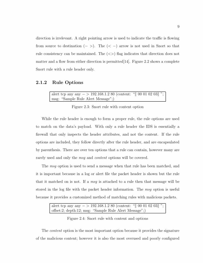
The content option is the most important option because it provides the signature

of the malicious content; however it is also the most overused and poorly configured

10

part of the rule[13]. Matching on the content is the most computationally expensive

portion of Snort and poorly designed content sections can substantially slow down

Snort. This being said, the content has several flags within it to provide better

customization to lessen the time required to search.

A signature is not always found at the beginning of a packet. Sometimes it is found

in the middle. The offset flag is used to specify where in the packet the malicious

content will begin. By using this flag, a large amount of time can be saved by skipping

data that otherwise would have been scanned. An offset of 10 would tell Snort to skip

the first 10 bytes of the payload before scanning. For more precision Snort provides

a way to specify the depth of the content using the depth and distance flags. The

depth and distance flags indicate the number of bytes to scan for a pattern match.

The main difference between the depth and distance flags is that depth is referenced

from the beginning of the packet, where distance is referenced from the last pattern

match. This is useful because in some attacks the signature can be found only within

10 bytes of the offset, and instead of Snort starting at the offset and scanning the

entire packet it can save time by only scanning the 10 bytes after the offset.

Sometimes malicious data is formed in a way that n bytes are between each

malicious signature. Snort has a flag within which specifies that the next signature

must appear within n bytes. Even with all these customizations, sometimes attacks

occur where the case (upper-case or lower-case) of the attack is irrelevant. Instead

of writing the same version of a rule with different cases the nocase flag is used. It

indicates that the case does not matter and if any match is found with that content

to send an alert. The content section has many optional flags in order to meet

the changing formats of attacks while maintaining the ability to search the payload

efficiently.

11

2.2 Snort Content Matching Process

The detection engine contains two content matching phases, the initial phase, and

the verification phase. Since Snort has complex rules with many options, a heavy

amount of overload is introduced. In order to reduce the overhead, Snort uses the

initial search phase to find possible rule matches. The initial phase ignores all content

flags and only searches for the largest content pattern within each rule. By ignoring

all flags, Snort significantly reduces overhead because it only needs to keep track

of the pattern matching algorithm. The initial phase algorithms are Boyer-Moore-

Horspool, Modified-Wu-Manber, and Aho-Corasick. Each rule match in the initial

phase is stored and once the initial phase is over they are sent to the verification

phase.

In the verification phase, Snort uses only the rules matched in the initial phase.

For each rule the verification phase uses all content options and flags to verify the

match. This phase introduces a large amount of overhead because several pointers

have to be maintained to keep track of positioning within the payload. Snort uses

Boyer-Moore-Horspool to verify the matches, because it is one of the fastest single

pattern matching algorithms. By splitting the search into two phases, Snort reduces

the overhead because the initial phase quickly prunes out all bad matches, while the

verification phase verifies a limited number of rules.

Chapter 3: Snort Content Matching Algorithms

As described in Chapter 1 and Chapter 2, Snort is primarily used as a misuse

detection system. During the content matching phase, the system compares the

packet payload with rules found in a signature file. To find matches, the default

algorithm in Snort is the Aho-Corasick string matching algorithm. However, different

variations of that algorithm and other pattern matching algorithms can be selected. In

the future, Snort plans on deprecating the use of the Wu-Manber search algorithm in

favor of faster algorithms that use less memory[16]. This chapter will cover alternative

algorithms and Snort’s version of Boyer-Moore, Wu-Manber, and Aho-Corasick.

3.1 Boyer-Moore Algorithm

The Boyer-Moore algorithm is fairly easy to understand. Its general idea is to skip as

many characters as possible without missing a possible instance of the string being

searching for. Snort uses a modified version of the algorithm called Boyer-Moore-

Horspool, because it uses less memory and suffers no significant speed loss[12]. Boyer-

Moore uses two tables (shift, bad character) and the text, whereas Boyer-Moore-

Horspool uses only one table (bad character shift).

In Snort the Boyer-Moore-Horspool algorithm[7] is rarely used in the initial con-

tent search unless there are fewer than five signatures, but it is used for the verification

search to find a match.

The Boyer-Moore-Horspool algorithm works as follows. Assume there is a pattern

pat with a length patlen. There is the original text text with a length textlen. The first

step is to precompute a shift table shift that tells the algorithm how many characters

12

13

it can shift given a particular value in pat. The shift table’s length shiftlen is the

size of the alphabet the algorithm is using, which can range from the entire ASCII

character set to a simple binary set.

The shift table is constructed as follows: pat[patlen − 1] is given a value of 1,

pat[patlen − 2] is given a value of 2, until finally pat[1] is given a value of patlen - 1.

patlen−1∑

i=1

pat[patlen − i] = i if pat[patlen-i] not in shift.

For each value in shift, if a value has already been computed then the shift table

will not be altered. For example in the pattern “its” the shift table would read shift[s]

= 3, shift[t] = 1, and shift[i] = 2. If the pattern was “iss” it would read shift[s] =

1, shift[s] = 1, and shift[i] = 2. Once all the characters present in pat have been

initialized a value, the rest of the characters in shift are given a value of patlen.

Once the shift table is computed the algorithm is ready to begin its search. Initially

pat is left aligned with text such that pat[1] is aligned with text[1]. The search always

begins at the right most character, so that the maximum number of characters can

be skipped in the event there is not a match. To begin the search the character

at text[patlen] is compared against the character at pat[patlen]. If the characters

do not match and that character does not exist in pat the algorithm shifts pat over

patlen such that the next compare will be text[2 ∗ patlen] against pat[patlen]. If a

match is found the algorithm begins comparing each character, and moves left by one

character each time a match is found. It will continue this process until a match is

either found or not found. On the event of a match not being found the algorithm

will make a call to shift and determine how many characters to move to the right.

For example, if pat[patlen] matches with text[patlen], the pointer will shift to the left

and compare pat[patlen − 1] with text[patlen − 1]. If this match fails the algorithm

will make a call to the shift table at pat[patlen − 1] and move that many positions

14

to the right. According to research done by Richard Cole, Boyer-Moore and Boyer-

Moore-Horspool have an average case complexity of O(n), where n is the length of the

text being searched[8]. Below is an example of the Boyer-Moore-Horspool algorithm,

being used to search for “mat” in the text “testtexttosearchon”.

pattern = mattext = testtexttomatchonshift = t = 0, a = 1, m = 2

m a tt e s t t e x t t o m a t c h o n

There is no match when comparing t with s, so a call to shift[s] is made and the

pattern moves to the right three characters and begins its next compare.


Again there is no match when comparing t with e so a call to shift[e] is made and

the pattern moves right three characters and begins its next compare.


Initially there is a match between pat[t] and text[t], because the characters are the

same. The algorithm moves to the left one character and compares the next characters

a and t. Since they are different a call to the shift table is made at shift[t] and the

pattern moves to the right by three.


After the pattern moved three positions to the right, a compare is made between

the characters a and t. Since there is no match, a call to the shift table is made at

shift[a] and the pattern moves to the right by one position.


15

Once the pattern moves one more position, it finds a match on the first group of

characters. The algorithm moves to the left one character at a time until it reaches

the final set of characters; the match is found and the algorithm is complete.

3.2 Wu-Manber Algorithm

The Wu-Manber algorithm [27] is based on the Boyer-Moore algorithm, except it

was created to support multiple pattern searches in one step. Since there are many

patterns searched for at once, it would appear that the algorithm should not take

large shifts because the probability of the last character of any pattern matching the

last character in the text is high. By using hash tables and other techniques, the Wu-

Manber algorithm is able to avoid this problem. The algorithm’s stages are described

in the sections below.

3.2.1 Preprocessing Stage

The first step in the Wu-Manber algorithm is to preprocess the set of patterns. This

step is truly beneficial if the same set of patterns is always used, because the prepro-

cessing can be done, saved to a file, and reread when needed. The preprocessing is a

fast process, and for most applications it can be completed during program runtime.

During the preprocessing stage three tables are built, a shift table, a hash table, and

a prefix table. The shift table is very similar to the shift table in Boyer-Moore, as

it is used to determine how many characters to shift when the text is scanned. The

hash and prefix tables are used to determine which pattern is a possible solution for

a match and to verify a match.

The first step in the preprocessing stage is to compute the minimum length of all

patterns patlen. All patterns are then forced to operate at the same length, which

can aid or hinder the efficiency of the algorithm. Having pattern lengths of similar

16

sizes will aid the algorithm because it will be able to shift the length of the smallest

pattern and most of the length of the largest pattern. Imagine a set of patterns that

have the lengths (5, 15, 7, 23, 10, 12). In this case patlen would be 5, which would

limit the maximum shift to be 5, thus reducing the speed of the algorithm. If the

set of patterns had lengths of (10, 12, 11, 9, 12, 13), the patlen would be 9, and the

algorithm can nearly shift the length of each pattern in the event of having no match.

Instead of sequentially looking at each character, the algorithm looks at blocks of

size B. In practice B typically is set to the value of two or three, however it is shown

that when M is the sum of all patterns, and c is the size of the alphabet, logc2M is

a good value[27]. The difference between the Boyer-Moore shift table and the Wu-

Manber shift table is that the Wu-Manber table determines the shift value based off of

the block size B, whereas Boyer-Moore determines the shift value by using the value

of 1. Other than the shift size variation, the shift table operates exactly the same as

the Boyer-Moore shift table. In order to compute the shift table the algorithm goes

through a two step process. The first case is if a character in the alphabet does not

appear in any pattern pat. If the character is not found then the shift value is patlen

- B + 1. If the character is found to be in the pattern then the algorithm assumes

that the value pos is the position of the last occurrence of that character value in all

patterns. The shift value will then equal patlen - pos + 1.

If the shift value equals 0 then a match is found, however the pattern which

matches is not initially known. The hash table is used to avoid searching every

pattern in sequence until the pattern that could be a possible match is found. For

the shift table, an index was computed, and this index is used for the hash table.

The ith entry in the hash table contains a pointer of a list of patterns whose last B

characters hash into i. Typically, the hash table is sparse because it holds only the

patterns, whereas the shift table holds all possible strings of size B.

17

To make more sense of everything, assume there is a shift table shift, a hash table

hash, and a hash value of the current suffix h. In the event of an initial character

match, shift[h] will equal 0; hash[h] contains a pointer to a list of possible patterns

that are used for the search.

The Wu-Manber algorithm introduces one more table called a prefix table. The

prefix table is used to speedup the processing when collisions are discovered. In the

same manner that the hash table is filled, the prefix table is filled except with the first

B characters of each pattern. When a collision is encountered the pointer in the text

is shifted patlen - B characters to the left. Those B characters are then compared with

the prefix table and this typically rules out a large number of patterns, because it is

rare that a pattern will have the same prefix and suffix. Once each table is computed

the preprocessing stage is complete. The preprocessing stage appears complex and

difficult to compute. However, it has been shown that with each table set to the size

of 215 and 10,000 patterns the preprocessing time is only .16 seconds[27]. This time is

truly insignificant considering a typical Snort implementation has 5,000 patterns, and

can be stored pre-execution. Once the preprocessing is complete, the actual search

stage begins.

3.2.2 Searching Stage

Once the preprocessing is completed the actual search algorithm is simple. The first

step is to compute a hash h based on the current position in the text text. If the shift

value is greater than zero, then the algorithm goes back to the first step. If the shift

value is zero the algorithm computes the prefix hash of the current section of text. If

the section of text is found to match a value in the prefix and hash table, then it is

searched directly. If a match is not found in both the prefix and hash table then the

algorithm goes back to the first step. The complexity of the Wu-Manber algorithm is

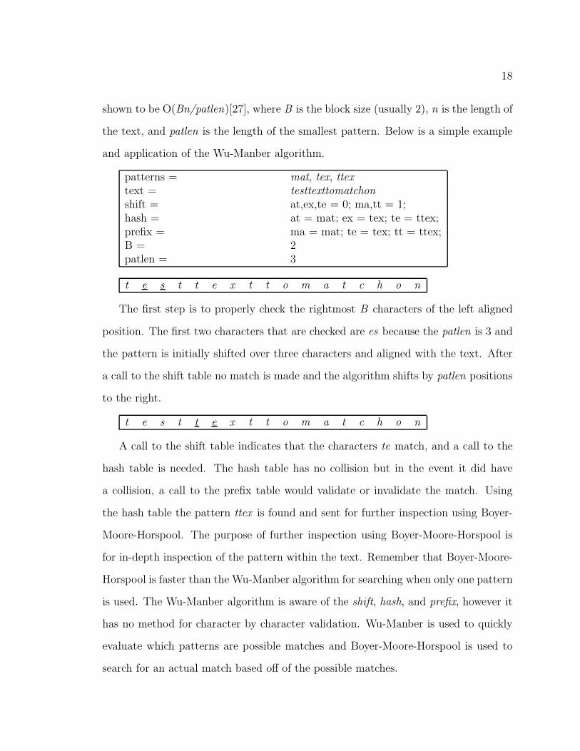
18

shown to be O(Bn/patlen)[27], where B is the block size (usually 2), n is the length of

the text, and patlen is the length of the smallest pattern. Below is a simple example

and application of the Wu-Manber algorithm.

patterns = mat, tex, ttextext = testtexttomatchonshift = at,ex,te = 0; ma,tt = 1;hash = at = mat; ex = tex; te = ttex;prefix = ma = mat; te = tex; tt = ttex;B = 2patlen = 3

t e s t t e x t t o m a t c h o n

The first step is to properly check the rightmost B characters of the left aligned

position. The first two characters that are checked are es because the patlen is 3 and

the pattern is initially shifted over three characters and aligned with the text. After

a call to the shift table no match is made and the algorithm shifts by patlen positions

to the right.


A call to the shift table indicates that the characters te match, and a call to the

hash table is needed. The hash table has no collision but in the event it did have

a collision, a call to the prefix table would validate or invalidate the match. Using

the hash table the pattern ttex is found and sent for further inspection using Boyer-

Moore-Horspool. The purpose of further inspection using Boyer-Moore-Horspool is

for in-depth inspection of the pattern within the text. Remember that Boyer-Moore-

Horspool is faster than the Wu-Manber algorithm for searching when only one pattern

is used. The Wu-Manber algorithm is aware of the shift, hash, and prefix, however it

has no method for character by character validation. Wu-Manber is used to quickly

evaluate which patterns are possible matches and Boyer-Moore-Horspool is used to

search for an actual match based off of the possible matches.

19

The one match with characters te is found but the algorithm continues, and moves

to the right by 1 position. Depending upon the application, the Wu-Manber algorithm

can be altered to quit searching once one match with one pattern is found. In an IDS,

the searching continues even after a match is found so that all matches will be alerted

and/or logged. This does not affect the IDS, because upon a true match the packet

will never pass through the system. If the packet is not going to pass through, it does

not matter it if is dropped in two seconds or ten seconds.


A call to the shift table indicates that the characters ex match, and a call to the

hash table is needed. The hash table indicates it has a match and the pattern tex is

sent for further inspection. The algorithm moves one position to the right, continues,

eventually finds mat, and ends once the entire text is searched.

3.2.3 Modified Wu-Manber

Snort actually uses a variation of Wu-Manber referred to as Modified Wu-Manber.

It occurs frequently that an intrusion detection system has a one byte pattern. The

typical Wu-Manber algorithm would compute a hash table and the block size B would

equal 1. This means that the maximum number of characters the algorithm could

shift is 1. If the typical block size of 2 is used, it would cause an out of bounds error

because some patterns are shorter than 2 bytes. In order to remove this problem

Snort creates either one or two hash tables depending on the pattern lengths. If

all 1 byte patterns are in the signature file, then one hash table is created for all

patterns which is known as one-byte hash. If the signature file contains both 1 byte

patterns, and patterns longer than 1 byte then Snort creates two hash tables. The

one-byte hash table contains all 1 byte patterns, and the second hash table known

as the multi-byte hash table contains all patterns greater than one. The Modified-

20

Wu-Manber algorithm removes the prefix table. This method speeds up the search

if there exist 1 byte patterns and multiple byte patterns. The 1 byte patterns are

searched for in a special Wu-Manber hash, while the multiple pattern’s shift size is

increased because the 1 byte patterns are removed.

3.3 Aho-Corasick Algorithm

The default algorithm for Snort is the Aho-Corasick algorithm. The basic idea is

to construct a finite state machine based off of patterns, and then to use that finite

state machine to process the text in one pass. Aho-Corasick operates by using three

basic functions which are the goto, failure, and output functions. The Aho-Corasick

algorithm operates linearly in the size of the input, which means that its complexity is

O(n), where n is the size of the text being search on[1]. Beyond these three functions

the algorithm can be simplified by converting it to a deterministic finite automaton

(DFA). The DFA can theoretically allow for a 50% reduction of transitions[1]. Each

reduction of a transition removes one extra compare and by reducing compares the

algorithm should process faster. A transition occurs when the function moves from

one state to the next. In practice the theoretical reduction is never achieved because

most of the time is spent in the start state.

3.3.1 Goto Function

The goto function’s purpose is to map a state and an input symbol to a state or to

fail. The first step in the goto function is to construct a goto graph. The graph starts

with only one vertex which represents the state 0 (the start state). Each character in

a pattern is added to the goto graph as a state, by adding a directed path starting

at the start state. New vertices and edges are added to the goto graph as needed

such that there is a path that can create the original pattern. The goal is to have

21

the minimal amount of states and transitions from the given set of patterns. If the

pattern is found in the text then the goto function returns the accept state and if

there is no arrow to move on to the next character the goto function returns fail. In

order to complete the construction of the goto function a final transition is added

from the start state back to the start state. This loop will ensure that the goto

function will continue to move back to itself when invalid input characters are used.

On completion of the loop, the goto function is complete and the failure function is

ready to be computed. In order to get a better understanding, a description of the

process of construction of the Goto graph in Figure 3.1(b) is provided below.

The first step is to take the patterns (mat, tex, ttex) and create a start state. The

state 0 represents the start state. The next step is to take the first pattern and create

a state and transition for each character. Transition “M” leads to state 1, transition

“A” leads to state 2, and transition “T” leads to state 3. The next step is to take

the second pattern, determine if it can be created from any current states, and if not

create new states and transitions. For the second pattern, no existing states could

be used so three new states and transitions were created. Starting at state 0 a new

transition “T” leads to state 4, transition “E” leads to state 5, and transition “X”

leads to state 6. The final step is to include the last pattern into the goto graph. The

last pattern optimally can be included by adding two transitions and one extra state.

A transition of “T” from state 0 to state 4 already exists for the pattern “ttex” to

use. There is however no transition of “T” from state 4 to any other state so one

must be added. A transition of “T” is added from state 4 to new state 7. Finally a

new transition of “E” can be used to take state 7 to state 5.

22

patterns = mat, tex, ttextext = testtexttomatchon

(a) data

0

6

32

5

7

4

1m a t

t

e x

t e

(b) Goto Graph

i 1 2 3 4 5 6 7f(i) 0 0 4 0 0 0 4

(c) Failure Function

i output(i)4 mat6 tex, ttex

(d) Output Function

Figure 3.1: Aho-Corasick Functions

3.3.2 Failure Function

The purpose of the failure function is to map a state into another state. The failure

function is called whenever the goto function fails. The construction of the failure

function begins once the goto function is complete, because it is built off of the goto

function. The failure function relies upon the depth of each state. The depth for a

state s can be computed as the length of the shortest path from the start state to s.

The failure function is computed for all states with depths starting at 1 because the

states are the inputs to fail not the depths. No failure function is defined for the start

state, because it should never fail. The output of the failure function is the state to

go to when no match is made. Assume there is a failure function f(),and a state s

23

with a depth d. For each state with a depth of 1, f(s) equals the start state. Once

the output for each state s at depth d is computed, d is incremented and that level

can be computed based off of the previous level’s non fail states of f(s). In particular,

each state of d (where d is greater than one) follows two basic rules. Assume we

have a state r, a goto function g, and a symbol a. For d - 1, if g(r,a) fails for all a

then do nothing. If it does not fail then for each new state q run f(q) until a value is

returned such that g(q,a) does not fail. Finally f(s) is set equal to g(q,a). In order to

understand the operation of the failure function, Figure 3.1(c) is described below.

The first step in computing the failure function is to take all states of depth 1 and

make their fail state 0. There are only two states, 1 and 4, with a depth of 1, so f(1)

= 0 and f(4) = 0. The next step is to use already created failure functions to form

the next depth. There are three states at depth level two, states 2, 5, and 7. For state

2, the algorithm determines if the failure state of f(1) can enter another state besides

itself using the symbol a, or if f(2) = g(0, a) ! = 0. No other state can be reached so

f(2) = 0. Following this logic the same happens for f(5) because f(5) = g(0, e) = 0.

For f(7), the algorithm determines if there is a transition of “T” from state 0. It turns

out that there is a transition of “T” to state 4 so f(7) = g(0, t) = 4. The last step is

to compute the state of depth 3, and they are computed as follows; f(3) = g(0, t) = 4

and f(6) = g(0, x) = 0.

3.3.3 Output Function

Associating a set of patterns with every state is the goal of the output function. The

first step of the output function is constructed at the same time as the goto function.

The pattern is added to the output function at the state that the pattern terminates.

The next step in the output function is computed during the failure function. When

it is found that f(s) equals some other state r, the initial outputs of states and r are

24

merged. As shown in Figure 3.1(d) all output values for this example are created at

initial construction.

3.4 Alternative Content Matching Algorithms

A significant amount of research has been put into finding alternative content match-

ing algorithms that are designed for specific applications such as IDS. Snort uses well

known algorithms for pattern matching, however it does not use algorithms geared

specifically to IDS needs. Several improvements have been made for all three major

Snort content matching algorithms. Even with these improvements the nature of the

algorithms limits the improvements to show only minimal speed gains. Three al-

ternative algorithms, Dual-Algorithm, Piranha, and E2xb have shown improvements

in speed gained, during the content matching phase, beyond at least one of Snort’s

default algorithms. These algorithms will be described in the sections below.

3.4.1 Dual-Algorithm

The Dual-Algorithm[26] comes from the observation that when the majority of pat-

terns in a rule group are multiple bytes, the addition of few one-byte patterns slow

the searching down. The Dual-Algorithm introduces the idea of a gapped ruleset. A

gapped ruleset is when there are rules of size n-1 and n+1 but none of size n. For

example, if a ruleset has rules of size one and three but none of size two, this is known

as a gapped ruleset. The Dual-Algorithm attempts to reduce the number of calls to

the Wu-Manber multi-byte hash table and it only works if there are both one-byte

and multi-byte patterns.

The algorithm starts by dividing the rule set into 2 subgroups, subgroup A and

subgroup B. Subgroup A contains all the one-byte patterns, and subgroup B contains

all multi-byte patterns. If the number of one-byte rules are, what is described as

25

suitably small (less than 5 rules), they are searched using the Snort implementation

of Boyer-Moore. If subgroup A is large, then a specialized one-byte pattern only

version of Wu-Manber is used. The variant has the same operation as Wu-Manber

multi-byte table, except that it operates only with one-byte patterns. For subgroup

B the Wu-Manber multi-byte hash table is used.

3.4.2 Piranha

Piranha[2] is an algorithm designed directly for IDS use and its main idea is that if

the rarest substring of a pattern does not match, then the entire substring will not

match with the text. In order to “know” which portion of the pattern is the rarest,

statistical analysis is taken over time on traffic. Each partial or whole match on a

rule is recorded to determine which part of each rule has been matched on the least.

The initial step is to break up a rule into 32 bit subparts. For example the rarest

sub pattern “abcde” would be broken up into 2 subparts, “abcd” and “bcde”. Each

subpart of the pattern is indexed and linked to which rule it originated from. The

packet payload is broken up in the same fashion as the rule. Each subpart of the

packet is checked against each subpart of each rule. If the subpart matches, that rule

is triggered and sent to the next stage of the algorithm. In order to reduce a large

portion of false positives, if a match is found, the last two characters of the rule are

matched against its corresponding characters in the text. If these characters match,

the payload is sent to Snort for a further in-depth search. The authors report a 10%

to 25% speed gain when compared to modified Wu-Manber, and a three to four times

speed gain versus Aho-Corasick Banded[2].

26

3.4.3 E2xb

E2xb[4] is a second generation algorithm designed from the original algorithm Exb[15].

E2xb is designed for applications with a small expected input size and a small match-

ing probability, like an IDS. The algorithm is based off of a simple assumption that if

the input text is missing at least one character of the pattern then the pattern is not

a substring of the original text. The algorithm uses a cell map that maps a group of

consecutive characters from the input text. Each group of consecutive characters is

referred to as an element. The larger the element the lower the probability of finding

a false-positive, but a higher probability of degrading performance. The algorithm

searches for these elements, and upon finding an element it sends the text for further

processing using other algorithms such as Boyer-Moore-Horspool. E2xb can have up

to 36% speed gains, and in some situations it can have a performance increase by up

to 300%[4]. The main problem with E2xb is that it is outperformed by Boyer-Moore

when a small number of patterns are used and it is outperformed by Aho-Corasick

when a large number of patterns are used. A typical IDS has a ruleset length so that

E2xb shows speed gains, however a few IDS have a large number of patterns and

E2xb should not be implemented. Overall E2xb shows signs of improvement, but it

only shows positive speed gains with a limited ruleset size when compared to other

content matching algorithms.

Chapter 4: Parallel Content Matching

Sequential content matching algorithms have traditionally been used for intrusion

detection systems because they typically support network speeds of up to 100Mbps

and with optimization they can work with speeds up to 200Mbps[18]. Networks that

have high line speeds cannot use a traditional IDS and require the purchase of expen-

sive hardware. One method to avoid the high costs of replacing hardware is to use a

parallel IDS. A parallel IDS is an intrusion detection system that processes data in

parallel, whereas a distributed IDS monitors different data at different locations[19].

This chapter focuses solely on types of parallelism, parallel IDS algorithm implemen-

tations, and their impact upon performance.

There are two basic styles of parallelism, data parallel and function parallel[26].

The purpose of data parallelism is to distribute computing across multiple nodes. A

node is an entity that can process packets using an IDS. A node can be a processor, a

multi-core system, or even a network; however the structure of the node is independent

from the parallelization method.

The main idea behind data parallel for an intrusion detection system is the same

idea behind a data parallel firewall[11]. Packets are distributed in such a fashion that

each packet is only scanned by one node. The benefit of the data parallel method is a

reduction of the arrival rate to each node, not a reduction of scanning time. Function

parallel is the idea that either the same or different data are being processed uniquely

per node. The benefit of function parallelism is that it reduces the processing time

for each node; however it does not reduce the arrival rate to each node.

27

28

4.1 Content Matching Parallelism

Since the bottleneck in Snort is during the content matching phase, it is important

to reduce the work during this phase. In content matching parallelism, the packets

will be forwarded to each node (function parallel), or certain nodes (data parallel).

In a data parallel IDS, the content matching phase can be distributed so that each

node receives approximately 1/n of the preprocessed packets, where n is the number

of preprocessed packets. In a function parallel IDS, the content matching phase work

is reduced because the rule groups are evenly distributed across all nodes. For the

content matching phase to function properly, it is important that each node process

the packets independently. Several methods of content matching parallelism have

previously been implemented including function and data parallel methods.

4.2 Function Parallel

As described earlier, function parallel is the method in which the data is distributed

to all nodes, but each node processes that data differently. Typically function par-

allel methods take less time processing, because processing is divided up among all

the nodes. Two function parallel techniques have been previously implemented, the

spread hash-group and function parallel Dual-Algorithm[26].

The purpose of the spread hash-group algorithm is to function parallelize the Wu-

Manber algorithm. This technique works with all Wu-Manber hash tables. The idea

behind this method is to spread non-empty hash table entries across nodes. The effect

is that each node has less to search for per packet. By reducing the number of hash

values, it decreases the number of distinct characters per node. By doing this, there

is a higher probability that each node will be able to skip a higher portion of the data

when no match is found. Also, decreasing the number of hashes at each node reduces

29

the number of hash table calls, and this should increase performance. In practice

this method proved to not show signs of much improvement. Using two nodes this

algorithm saw a 1.12 speedup, while using four nodes it saw a 1.20 speedup[26]. The

speedup of this approach is limited because as more rules are added the speed lost is

insignificant. This means that the time to search through hash tables with 20 rules

or hash tables with 100 rules will be relatively the same. The hash-groups are spread

across each node, but since the size of the hash is insignificant to the search time,

each node’s time is basically the same as if it had the original ruleset.

The other function parallel technique was based on the Dual-Algorithm. This

method differs from the previous approach in that different nodes have completely

different functions. One node processes only the one-byte patterns. Typically the

algorithm used is Boyer-Moore, but if a large number of one-byte patterns are in

the rule groups, then Wu-Manber is used. The other node uses all large patterns in

the rule file to process its packets. By separating the work, the one-byte patterns

should complete quickly, and the large group should also complete quickly because

it is able to shift more for each match failure. A limiting factor to this technique is

that only two nodes can be used. In an IDS with more nodes there are several ideas

for parallelization. If a large number of one-byte patterns are present, they could be

broken up so that each node has a small enough number on which to apply Boyer-

Moore. Further, the large patterns could be broken across nodes in the same fashion

the spread hash-groups algorithm did.

In the original idea, speedup for the two node implementation was 1.96 times[26].

This method has the greatest speedup for two nodes; however since it cannot be used

with more than two nodes, its scalability is greatly reduced. Using the modifications

mentioned will provide scalability to more nodes. As more nodes are added, the

speedup will resemble the leveling trend of the spread hash-group time.

30

4.3 Data Parallel

As previously mentioned, data parallel is the technique in which each piece of data is

scanned by only one node, and that all the data is distributed in a round robin fashion

via a splitter. Previous work has implemented data parallel methods using both the

Wu-Manber and Dual-Algorithm[26], also, two approaches to data parallel IDS have

been previously implemented. One method uses a traditional packet distribution,

while the other divides up each packet and sends each fragment to a node. This

section will review the previous implementations and their benefits and weaknesses.

4.3.1 Traditional Data Parallel using Wu-Manber

In previous work[25, 26], data parallel algorithms were tested using the Snort Wu-

Manber implementation. In [26] the Wu-Manber algorithm was run traditionally

using two and four nodes. The results shown were for the actual time to search and

not the preprocessing. Preprocessing includes the time to distribute packets to each

node. The actual implementation involved using trace files and dividing the packets

among all nodes. To avoid the problem of different nodes reading from the same

location, each node had its own preprocessed Wu-Manber structure and preprocessed

set of rules. For two nodes the Wu-Manber algorithm saw a speedup of 1.94, and

with four nodes it saw a speedup of 3.48. The search time for the parallel content

matching phase using the Wu-Manber algorithm nearly followed theoretical rates[26].

4.3.2 Data Parallel Dual-Algorithm using Wu-Manber

Not only was the Dual-Algorithm tested using sequential methods, it was tested after

it had been implemented in a data parallel IDS. In [26] it was implemented using the

same two and four nodes as the traditional data parallel method. The implementation

of the Dual-Algorithm followed the idea that each node had its own set of structures.

31

The rule set that was used only had two one-byte patterns (typical among IDS), so

for each node, Snort’s Boyer-Moore algorithm was used to find only those pattern

matches. Each node had its own Wu-Manber multi-byte hash table and shift table,

so no node would attempt to read from the same location. Each node used its copy of

the multi-byte hash table and shift table to search for patterns that were of length two

or greater. Each node was given unique packets, in a round robin fashion, to process.

Compared to the default Snort algorithm the two node Dual-Algorithm data parallel

had a 2.27 speedup, whereas the four node implementation had a 4.29 speedup[26].

4.3.3 Data Parallel using Packet Division

The work of Boss and Huang[6] introduced a new data parallel approach. The ap-

proach involves breaking each packet as it enters the network. Instead of sending an

entire packet to each node in a distributed fashion, a fragment of each packet is sent

to most nodes. This approach contains both a function and data parallel advantage.

Like a traditional data parallel approach, different data is sent to each node; however

the arrival rate is decreased because most nodes see a portion of each packet. Work

is reduced at each node, not by decreasing the number of rules, but by decreasing the

content that the rules need to match on. Figure 4.1 is an example of a data parallel

system that divides packets and distributes them to all nodes.

As packets are divided, a problem can occur in that a malicious pattern is also

divided. If the malicious packet is divided, then the current IDS will be unable to

detect it. In [6] a method referred to as “spilling” is introduced to avoid this problem.

As shown in Figure 4.2, an overlap of data is added to each fragment so that each

node will find all malicious patterns that existed in the original packet payload. The

size of overlap per split is the length of the maximum pattern minus one.

Unfortunately in this method additional data is required to be scanned at each

32

Traffic Splitter

Frag 1Frag 0 Frag 3Frag 2

PacketPacket

Frag 2Frag 1Frag 0

Node 3Node 2Node 1Node 0

Packet1

Packet0

Figure 4.1: Data parallel system using packet division

Original Packet Length

Overlap

(Maximum Pattern Length – 1)

Figure 4.2: Packet overlap

node which slows the IDS compared to a traditional data parallel approach. Figure

4.2 is an example of a packet and its overlap or “spilling” section.

In [6] data parallel with packet division is introduced, however it is never tested

for its performance. The work in [28] alters the “spilling” method introduced in

[6]. Instead of evenly distributing the overlap across the two fragments, the overlap is

distributed only on the right fragment. This method unevenly distributes the overlap,

because the last fragment will contain no overlap. Tests were run on an IXP board

with eight nodes and results showed that with eight nodes the algorithm can obtain

33

up to a 60% decrease in processing time.

Original Packet

(Time to Scan = 160ms)

Sequential Scan

(Time to Scan 30ms upon match)

Scanned

Portion

Scanned Portion

(no match 40ms)

Scanned

PortionScanned Portion

(no match 40ms)

Scanned Portion

(no match 40ms)

Packet Length 200 bytes

Figure 4.3: Data parallel system without synchronization

To understand how the system worked, their implementation of data parallelism is

shown as follows. Each packet is split into fragments via a traffic splitter; the split is

based on the size of the packet and the number of nodes in the system. Each fragment

is sent to a node determined by the splitter and the content matching phase starts.

The content matching phase then operates the same as the sequential scan. In certain

implementations, when a malicious pattern is found the search scans the rest of the

packet and the packet is not dropped till the end of the content matching phase. In

this implementation once a malicious pattern is found, the packet is dropped from

the network. The problem with this approach occurs when a match is found in any

fragment other than the last. In Figure 4.3, the sequential system finds a match in

the first part of the packet (30ms), stops scanning, and drops it from the network.

In the [28] system the first node finds a match and stops scanning(30ms). The rest

of the nodes continue scanning their portions of the packet(40ms). In this instance

the sequential system is doing less work than the data parallel system overall. The

sequential system is done scanning in only 30ms whereas the data parallel system is

done scanning in 40ms. The amount of data scanned in the sequential system was 38

out of 200 bytes whereas the data scanned in the data parallel system was 188 out of

200 bytes. Upon seeing this case, which is common in an IDS, it is apparent why the

system in [28] fails to reach the speed of a traditional data parallel system.

34

The benefit of the data parallel algorithm in [6, 28] is that work is distributed

among nodes so that each node has to do less work. The main problem with this

approach is that while data is divided, data overlap is introduced which slows down

the IDS. Neither work provided any other performance enhancement to overcome the

time lost by adding data to each fragment.

Chapter 5: Divided Data Parallel Method

Previous work [6, 25, 26, 28] has shown improvements for data parallel methods in

an IDS. With increasing network speeds it is important to not only come up with an

approach that works, but an approach that outperforms all previous methods. The

work in [25, 26] has shown the largest speed gains; as the number of processors n

increases, the time to scan for a packet approximately decreases at a rate of n. A

decrease in scanning rate is achieved when the Dual-Algorithm is performed in a data

parallel fashion.

This chapter introduces a new method called Divided Data Parallel(DDP), which

is a divided-data data parallel approach based on the techniques mentioned in [6, 28].

The DDP method uses the overlap system with a synchronization array in order to

produce speed reductions greater than any other current parallel approach. Besides

speed, one large benefit of DDP is its independence of the content matching algorithm

used. Some parallel techniques require a certain content matching algorithm in order

to work[20, 26]. Because of its independence, as new improved sequential algorithms

are implemented, they can be quickly added to DDP. This chapter will first cover the

main techniques that make this method unique, and then it will talk about an overall

system design using DDP and the implementation of DDP.

5.1 False Negative Avoidance

As described in Chapter 4, data overlapping was introduced as a way to ensure all ma-

licious patterns are found. Without overlapping the intrusion detection system would

suffer from false negatives, in order to detect these, DDP also implements overlap-

35

36

ping. A false negative occurs when malicious data exists in the original packet, but

after splitting the packet and distribution the IDS is unable to detect that malicious

data. An overlap based algorithm works as follows. Upon determining a proper split,

the overlap is computed. After the split, both new fragments contain duplicated data

that equals the length of the maximum pattern maxpat minus one. The purpose for

subtracting one is so that both fragments will not read the same byte twice. For each

fragment in the system the first fragment will only contain maxpat/2 overlap bytes,

whereas the last packet will contain ceil(maxpat/2)−1 overlap bytes. Each fragment

between the first and the last will contain a total overlap of maxpat − 1. Figure 5.1

shows an example of the overlap for a system using four processors.

Original Packet

Frag 0

(Overlap = Maxpat/2)

Frag 3(Overlap = Maxpat/2 - 1)

Frag 2

(Overlap = Maxpat – 1)

Frag 1

(Overlap = Maxpat – 1)

Overlap

Figure 5.1: Packet split into four fragments, showing overlap

In order to get a better understanding of how packet fragmentation works, Figure

5.2 shows a real example that has a maxpat of 3 and a total of two processors.

The original packet has a length of 10 characters so the first fragment has the first 6

characters of the original packet whereas the second fragment has the last 6 characters.

The figure shows two different examples which indicate breaks when the pattern being

searched for is in a different location in the original packet. The final portion of the

figure shows what happens if the data was not overlapped. The pattern being searched

for in these examples is the phrase “pat”. For figure 5.2(a) notice that both fragment

37

one and two read characters “at”, which is the duplicate data maxpat - 1. In this

case the first fragment matches on the pattern. In Figure 5.2(b) the pattern “pat”

has been shifted over one character to the left. Now the duplicated data is “pa”,

and the second fragment finds the pattern. The last figure 5.2(c) shows an example

when no overlap is present. In this case the pattern being searched for is split across

both fragments. Since it is split, neither fragment one or two find the pattern, which

results in a false negative.

Original Packet: xxxpatxxxx

First Fragment: xxxpat

Second Fragment: atxxxx(a) First Example

Original Packet: xxxxpatxxx

First Fragment: xxxxpa

Second Fragment: patxxx(b) Second Example

Original Packet: xxxpatxxxx

First Fragment: xxxpa

Second Fragment: txxxx(c) Without Overlap

Figure 5.2: Example showing overlap in a 2 processor system

5.2 Synchronization Array

The work in [6, 28] introduced the overlap method, however it accepted the cost of

adding overlap without adding any method to reduce that extra cost. Since overlap

is used in the DDP method, extra data is forced to be scanned each time through the

system. This extra scanning results in increased search time that sets its speeds below

traditional data parallel speeds. In order to reduce the searching time throughout the

whole system, DDP uses a synchronization array to decrease the time needed to

search.

It is common that in a sequential content search, if a malicious pattern is found

the algorithm does not continue scanning the whole packet; rather it stops scanning

and drops the packet from the network. In a traditional data parallel approach the

38

whole packet is sent to a node. Since the whole packet is sent to the node a scan

operates the same as in the sequential system. At each node, if a malicious packet

is found, that packet is dropped from the network. The other data parallel approach

fragments each packet and distributes those packets to the nodes.

In order to prevent scanning the same data multiple times, a synchronization

component using shared memory is added to the DDP method. The synchronization’s

purpose is to keep as many nodes as possible from scanning a packet for which a match

has already been found. For each packet, a synchronization bit is initialized to “0” and

each fragment has a pointer to that bit. If one fragment finds a pattern match that

bit is flipped to a “1”. Before a scan, each node checks the fragment’s synchronization

bit, if it is “0” it scans, if it is a “1” it drops the fragment from the network.

At first glance this system would appear to work in only rare cases, because each

node should begin scanning at approximately the same time. If they begin at the

same time, then no node will have had time to find a pattern match in its fragment.

In an extremely underloaded system, this may be they case, because no node will

have a filled buffer and all nodes will process the same packet’s fragments at the

same time. In a loaded system each node will have its own buffer of fragments to

scan. Since it takes different times to scan different fragments it could occur that

one node is on the second packet’s fragment, whereas another node is on the fifth

packet’s fragment. In this situation, which is typical of an IDS, the synchronization

works. Different nodes scanning different packet fragments increases the probability

of a particular packet’s synchronization bit being flipped before another node starts

scanning another fragment from that packet. Figure 5.3 demonstrates the concept of

buffered synchronization.

In this figure there are multiple nodes, but only 2 are shown: node 0 (the first

node) and node n (the last node). Each node has a different buffer of fragments which

39

Node 0(retrieving frag 2.0

from buffer)

Node n

(scanning frag 2.n)

Frag 2.0

Frag 6.0

Frag 7.nFrag 5.0

Frag 6.n

Frag 5.n

Frag 3.n

Frag 4.0

Frag 3.0

Frag 8.n

Buffer 0

0

0

1

0

0

0

Figure 5.3: Synchronization with buffer

point to their synchronization bit. In this example, node n has just found a pattern

match in the fragment from packet 2 and has flipped its bit. Node 0 is getting ready

to scan its fragment from packet 2. Once it checks the bit, it will drop that fragment

from the network. This system can work well because, often, not every node has the

same buffer contents and the lack of similarity allows more fragments to be skipped.

5.3 Design of the DDP Method

The design for the DDP method starts the same as any parallel approach. The first

step in the system is to receive packets from either the network or a trace file, and

send them through Snort. For the purposes of testing and results, a trace file was

used instead of live network traffic because network traffic could not be generated

at high speeds. Once the packet enters Snort, the DDP method determines how to

fragment the packet. The maximum number of nodes maxnodes the system can use,

given a particular packet, is the packet length l, divided by the maximum pattern

length maxpat.

maxnodes = l

maxpat

If maxnodes is larger than the nodes in the system, then the nodes in the system

are used for the split, otherwise maxnodes is used. Once the number of nodes that

can be used is determined the packet is fragmented into equal portions. The next

40

step is to determine the overlap, and that method follows the same as the method

described in Section 5.1. At this point, each fragment is determined and has its

overlap computed. Once this stage is complete, a synchronization bit is created for

each packet, and each fragment links to its packet’s synchronization bit. The list of

bits is simply known as a synchronization array.

The next step in the approach assigns the fragments to the nodes. A random

distribution is used to distribute the fragments. A round robin splitter works well, but

it increases the probability that each node will work on the same packet’s fragments

at the same time. If each node is working on the same packet’s fragments at the same

time then more work will be done as fewer fragments can be skipped.

When using the synchronization array each node in the IDS could be described

as in a race condition. Normally race conditions are bad, but in this case we want

each node to skip as many packets as possible and race to the be first one to scan an

unmarked packet. Random distribution aids the race condition because it increases

the probability that each node will be scanning a different packet’s fragments. When

a round robin distribution is used, the DDP algorithm performs worse than when a

random distribution is used. Even though they both have approximately the same

number of packets per node, the packets in the random distribution contain a greater

disparity in order than the packets in the round robin system. The lack of order

ironically helps the synchronization array and allows the DDP method to complete

content matching even faster.

Once the distribution is complete, each node will scan for a content match. If that

match is found the synchronization bit will be flipped and the packet will be dropped

from the network. If a fragment has not been dropped there is a fragment reassembly

stage. Before the fragments are reassembled the synchronization bit is checked to see

if it was flipped. If the bit was flipped each remaining fragment is dropped and the

41

synchronization bit is freed. If the bit is not flipped all fragments are reassembled

and the synchronization bit is freed. Each node can have its own content matching

algorithm or they can all be the same; the content matching phase is independent of

the synchronization, overlap, and packet distribution. Figure 5.4 is an example of the

DDP system.

Traffic Splitter

Node 0

Frag 3Frag 1 Frag 0Frag 2Synchro

Bit

PacketPacket

Node 3Node 2Node 1

Figure 5.4: The DDP system

5.4 Aho-Corasick and Wu-Manber Content Matching Algo-

rithms

The DDP method is similar to data parallel in the fact that it is independent of the

content matching algorithm. Since DDP was implemented in Snort, the algorithms

it was tested on were Aho-Corasick and Wu-Manber.

For the Aho-Corasick algorithm, each rule group was duplicated across all nodes.

This means that each finite state machine that had been compiled with the rule set

was duplicated and distributed to each node. The important goal of node distribution

is to make certain nodes read from their own structure instead of each trying to read

from one structure. If they all read from the same structure it would serialize access,

which would essentially make the algorithm sequential. For Wu-Manber each hash

42

table was duplicated and distributed across all nodes in the same fashion the finite

state machine was. On average the Aho-Corasick algorithm outperformed the Wu-

Manber algorithm in the DDP system. The next chapter will show the experiments

and results for both algorithms.

Chapter 6: Experimental Evaluation of Parallel

Techniques

In order to compare the performance of DDP and other parallel methods, a shared

memory system is used. A shared memory system is not necessary but optimal con-

sidering the synchronization array used in DDP. In a cluster or multiple node system

a slower method of communication would need to be used in order to synchronize,

thus reducing the benefit of the array. The machine used for testing is a Linux ma-

chine running Gentoo TM, with four dual core processors. Two different rule sets are

used for testing to show that the results are consistent over different rule sets. This

chapter will outline the system used, the rule sets, speed results for all past parallel

approaches, and speed results for DDP including its variations.

6.1 System Design

The first rule set used is a default set of TCP rules from Snort 2.6.0 while the second

is a set of rules created by an IDS expert[26]. For each test, a group of trace files were

compiled from real network traffic that contained various TCP application data and

different packet sizes[26]. The trace files contain malicious and non-malicious data

that can match on the IDS rule sets. On both rule sets, the same trace files were used

so that the results are comparable. This section will explain the machine architecture

and each rule set in detail.

43

44

6.1.1 Linux System

The Linux system uses the Gentoo TM2.6.17 operating system. The system consists

of four dual-core AMD 64-bit processors. Using each core the system has eight 64-bit

processors that run at 1.8Ghz each. The system uses a shared memory architecture

and has 8 Gigabytes of memory. The kernel is configured so that no preemption is

used; this means the operating system will not halt or stop processes in favor of a

higher priority task. Preemption improves timing measurements because no other

process can interrupt and use timed clock cycles.

6.1.2 Default and Expert Rule Set

The default rule set was formed using the default rules Snort distributes with each

version. The rules were taken from the set of all rules from Snort 2.6.0 that apply

only to the TCP protocol. The final TCP rule set consists of 996 unique rules which

content sizes range from 1 to 80 bytes, which are shown in a histogram in Figure 6.1.

There are 34 patterns of size one, 94 patterns of size 2, and 47 patterns of size 3. The

majority of the patterns exist between the ranges of 1 to 24 bytes. There are a total

of 790 or 79 percent of the rules in this range.

The expert rule set is the same rule set that is used in [26]. This rule set was

created by experts at a national laboratory for web content only traffic. The rule set

consists of 344 rules whose patterns range from size 1 to size 80, which are shown in

a histogram in Figure 6.2. There are 2 one byte patterns, 3 two byte patterns and 15

three byte patterns. The majority of the patterns range from length 3 to length 16.

There are a total of 277 rules within that range. For most tests this rule set is used

because it was created by professionals and is not a default rule set that needs to be

pruned. As mentioned earlier, both rule sets are used, however the expert rule set

is used more often because it represents a rule set of a true implemented IDS. The

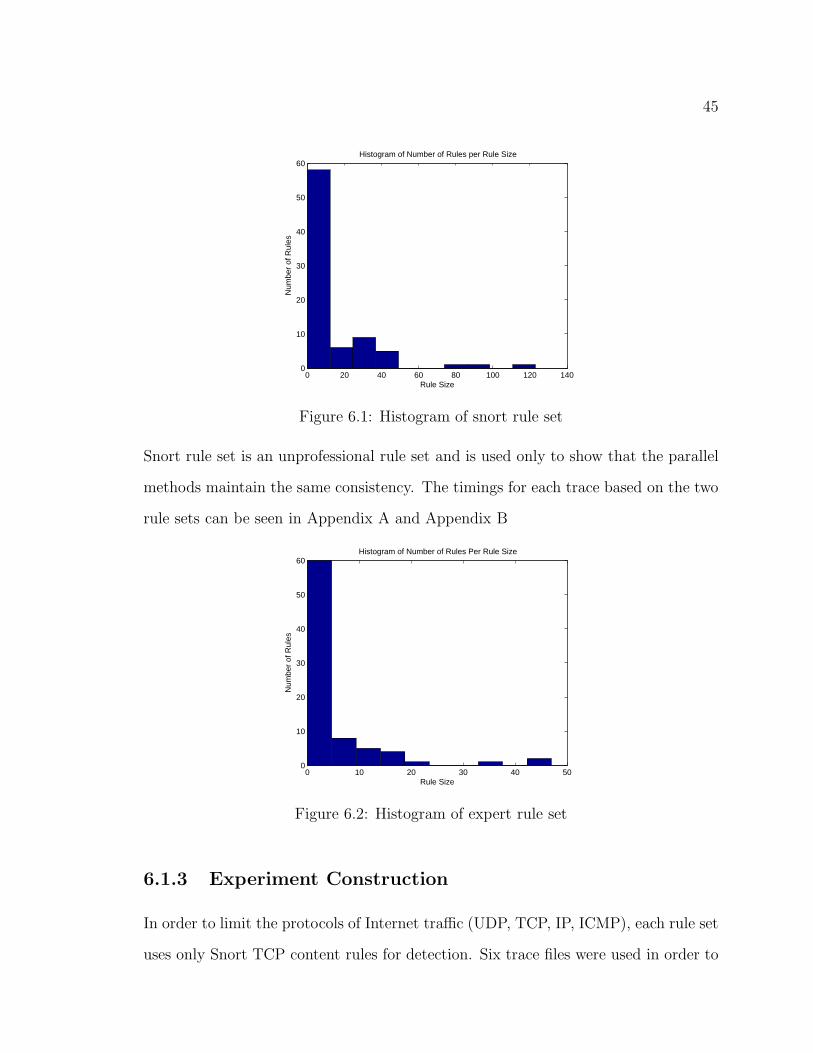
45

0 20 40 60 80 100 120 1400

10

20

30

40

50

60

Num

ber

of R

ules

Rule Size

Histogram of Number of Rules per Rule Size

Figure 6.1: Histogram of snort rule set

Snort rule set is an unprofessional rule set and is used only to show that the parallel

methods maintain the same consistency. The timings for each trace based on the two

rule sets can be seen in Appendix A and Appendix B

0 10 20 30 40 500

10

20

30

40

50

60

Rule Size

Num

ber

of R

ules

Histogram of Number of Rules Per Rule Size

Figure 6.2: Histogram of expert rule set

6.1.3 Experiment Construction

In order to limit the protocols of Internet traffic (UDP, TCP, IP, ICMP), each rule set

uses only Snort TCP content rules for detection. Six trace files were used in order to

46

show performance differences. Each trace file was generated using actual web traffic

from the University of California, Davis. During the capture phase the system only

accepts TCP packets and drops any other packet from the system. Since only TCP

packets are used, every packet will be compared against all rules in each rule set in

these experiments. This will provide consistency across trace files and rule sets.

In order to get results using these trace files, an accurate timing method is needed.

Snort preprocessing time is negligible compared to the time taken during the content

matching phase. For the purpose of these experiments the time will only be taken for

actual content matching and not for preprocessing and machine set up. In order to

achieve accurate timing, time is captured in nanoseconds. In order to do this, assembly

code is used. This method is multi thread and multiprocessor safe, meaning it will

get accurate timings even when multiple threads are used on multiple processors[26].

Each test completion actually consists of twenty runs and an average is taken for the

total time and σ (standard deviation) is computed. For the DDP method, several

more trace files were created to test certain aspects of the approach. These other

trace files are explained in the DDP method section in this chapter.

In order to verify that each parallel method is matching on the same number of

rules and the same rules, a method of counting is needed. For each match, a global

counter is incremented and the final counter value is stored. As each match is found,

the rule and text of the packet that the rule matches on is also stored. In order to

determine the parallel method’s integrity, the counter and matched rules need to be

the same as the values in the sequential search. In this system the integrity is verified

for each trace file and rule set.

47

6.2 Current Parallel Approaches

In order to test the efficiency of DDP, current parallel approaches first need to be

tested. Each test will be used to show the speed gain of the approaches using the

trace files and the Linux system. Each parallel algorithm mentioned in Chapter 3 will

be used as well as an extension to data parallel. The extension is that data parallel

using Wu-Manber is ported to use Aho-Corasick.

6.2.1 Data Parallel Extended with Aho-Corasick

The work in [25, 26] showed a data parallel approach using Wu-Manber. This method

had significant speed gains over other approaches. In order to test the effectiveness

of data parallel, the method was altered to handle the Aho-Corasick algorithm. The

function of the overall method works the same as other data parallel approaches.

1 2 4 6 81

2

3

4

5

6

7Speed Up Curve as the Number of Processors Increase

Number of Processors

Spe

ed U

p

Trace 1Trace 2Trace 3Trace 4Trace 5Trace 6

Figure 6.3: speedup curve with expert rule set

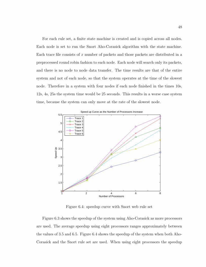
48

For each rule set, a finite state machine is created and is copied across all nodes.

Each node is set to run the Snort Aho-Corasick algorithm with the state machine.

Each trace file consists of x number of packets and those packets are distributed in a

preprocessed round robin fashion to each node. Each node will search only its packets,

and there is no node to node data transfer. The time results are that of the entire

system and not of each node, so that the system operates at the time of the slowest

node. Therefore in a system with four nodes if each node finished in the times 10s,

12s, 4s, 25s the system time would be 25 seconds. This results in a worse case system

time, because the system can only move at the rate of the slowest node.

1 2 4 6 81

1.5

2

2.5

3

3.5

4

4.5

5

5.5


Spe

ed U

p

Speed up Curve as the Number of Processors Increase


Figure 6.4: speedup curve with Snort web rule set

Figure 6.3 shows the speedup of the system using Aho-Corasick as more processors

are used. The average speedup using eight processors ranges approximately between

the values of 3.5 and 6.5. Figure 6.4 shows the speedup of the system when both Aho-

Corasick and the Snort rule set are used. When using eight processors the speedup

49

ranges approximately between 3.5 and 5.5. The expert rule set achieved a greater

maximum than the Snort rule set. The main reason for this is that the Snort rule set

contained 996 rules, and an increase in rules will minimally slow the content matching

process.

6.2.2 Data Parallel using Snort Wu-Manber

The layout of the data parallel approach using Wu-Manber is the same as the approach

using Aho-Corasick except the searching structures and algorithm is different. For the

trace file each packet is distributed among each processor in an untimed preprocessed

round robin fashion. Each node searches only its own packets, and the overall system

time is the same as the time of the slowest node. Below are two figures showing the

Wu-Manber data parallel method.

1 2 4 6 81

2

3

4

5

6

7


Spe

ed U

p

Speed Up Curve as the Number of Processors Increase


Figure 6.5: Wu-Manber speedup curve for the expert rule set

Figure 6.5 shows the speedup of data parallel using the Wu-Manber algorithm

when the expert rule set is used. With eight processors the speedup approximately

50

1 2 4 6 81

2

3

4

5

6

7


Spe

ed U

p

Speed Up Curve as Number of Processors Increase

Aho Trace 3Aho Trace 4Wu Trace 3Wu Trace 4

Figure 6.6: Graph that compares the speedup of Aho-Corasick verses Wu-Manber

ranges between 3.75 and 6.75. Figure 6.6 compares the Aho-Corasick algorithm with

the Wu-Manber algorithm, using the data parallel approach. Only two traces, 3 and

4, were chosen so that the graph could show the difference without confusion. In

the graph it is clear that the Wu-Manber algorithm outperforms the Aho-Corasick

algorithm. As more nodes are added, the Aho-Corasick algorithm loses performance

while the Wu-Manber algorithm’s percentage of increase stays relatively the same.

The reason for the performance results is because on average Wu-Manber outperforms

Aho-Corasick.

6.2.3 Data Parallel using Dual-Algorithm

The Dual-Algorithm system is distributed in the same manner as the previous two

data parallel systems. Each set of dual hashes are copied and distributed across all

nodes. The packets are distributed to the nodes in a round robin fashion. The Dual-

Algorithm is used to search each packet’s payload. The overall system time is the

51

time of the slowest node.

1 2 4 6 81

2

3

4

5

6

7


Spe

ed U

p



Figure 6.7: speedup Curve of the Dual Algorithm

Figure 6.7 shows the speedup curve of the data parallel Dual-Algorithm with the

expert rule set. The speedup with eight processors ranges between 4.25 and 6.25.

Figure 6.8 shows that the Dual and Wu-Manber algorithm have approximately the

same speed while Aho-Corasick has the worst. For trace 3 the Dual Algorithm out-

performed Wu-Manber but for trace 4 Wu-Manber outperformed the Dual algorithm.

As more processors are added the disparity between the algorithms is greater.

The Wu-Manber algorithm tends to perform the best overall because it has the

best average case performance of all three algorithms. The Dual algorithm is es-

sentially a modified version of the Wu-Manber that is intended for rule sets with

gaps. In the case of these rule sets there are no gaps so the Dual algorithm resem-

bles Wu-Manber. Aho-Corasick algorithm has the best worst case performance and

it outperforms the other two algorithms when worst case data is present. The worst

case data is when no matches are found on the given packet, so the entire set of rules

52

1 2 4 6 81

2

3

4

5

6

7


Spe

ed U

p


Aho Trace 3Aho Trace 4Dual Trace 3Dual Trace 4Wu Trace 3Wu Trace 4

Figure 6.8: speedup of Aho, Dual, and Wu

has to be searched against the entire packet. In these data sets this situation does

not frequently occur so Aho-Corasick shows worse performance.

In each one of these experiments the same data parallel method was used, but

the content matching algorithm was altered. The results show that some content

matching algorithms scale better with parallelism while others do not. According to

traditional data parallel methods, Wu-Manber scales the best, but with a few changes

in traffic patterns and rule sets other algorithms can perform better.

6.2.4 Function Parallel using Wu-Manber

The function parallel algorithm is the spread hash groups algorithm mentioned in

Chapter 3. Each hash table is evenly divided and spread across each node. The pro-

cess of division and distribution is part of preprocessing and therefore is not included

in the timing. At each node the packet’s payload is searched using the Wu-Manber

algorithm. At each node the Wu-Manber algorithm will only use the hash tables it

53

has locally. The packets are distributed in a duplicated fashion to all nodes during

preprocessing. The system time is the time of the slowest node. The times for the

function parallel runs can be seen in Appendix D.1.

1 2 4 6 81

1.01

1.02

1.03

1.04

1.05

1.06

1.07

1.08

1.09

1.1


Spe

ed U

pSpeed Up Curve as Number of Processors Increases

Average of Trace 1,3,4

Figure 6.9: speedup curve of the function parallel algorithm

Figure 6.9 is the average times of traces 1, 3, and 4 with the expert rule set. The

function parallel algorithm underperforms compared to the previous data parallel

methods. The reason it does not perform well is because of the scalability of the rule

sets. Snort has optimized the Wu-Manber algorithm so that as more rules are added

the time to search through those rules is sub linear. Therefore the cost of having 200

rules versus 50 rules is insignificant to the overall search speed. In this run the expert

rule set was used which has 277 rules. When two processors were used there are 138

rules on one machine and 139 on the other. Since there is a drop of over 100 rules per

machine there is a slight increase in speed. When four processors are used the four

machines get 69, 69, 69, and 70 rules. The drop is less compared than when using

two processors, therefore a lower amount of speed is gained. This process applies to

54

each increase in nodes, and results are shown in Figure 6.9. Since function parallel

performs so poorly it is ignored from future graphs, but it is still important to note.

6.3 Divided Data Parallel Method

For the DDP method several different modifications from previous algorithms are

used. During preprocessing DDP has several steps. The first part of the method is

to distribute the rule structures across all nodes. Since DDP can be used with both

Wu-Manber and Aho-Corasick, DDP will distribute the structure that is based on

the searching algorithm. The next step is to read in a trace file and determine where

each packet can be split. The method used for splitting and overlap is the same as

mentioned in Chapter 4. Once each fragment has been created, a synchronization

bit is stored and each fragment has a pointer to that bit. Finally, the fragments are

distributed to each node randomly and not in a round robin fashion.

Once preprocessing is complete the same method of timing as in the other parallel

algorithms is used. The timing is used only during the content-matching phase and

not for preprocessing or machine setup. Each node works on its own fragment and

the system time is the time of the slowest node. When synchronization is included,

however, each node tends to finish at approximately the same time because of the

skipping of packets.

The DDP method uses several different techniques for searching and is not as sim-

ple as the previous data and function parallel methods. Since DDP consists of several

elements, this section will discuss and show the results of including and excluding the

overlap and synchronization. Each part will include the effects while using both the

Wu-Manber and Aho-Corasick algorithms. The times for each method can be seen in

Appendix C.

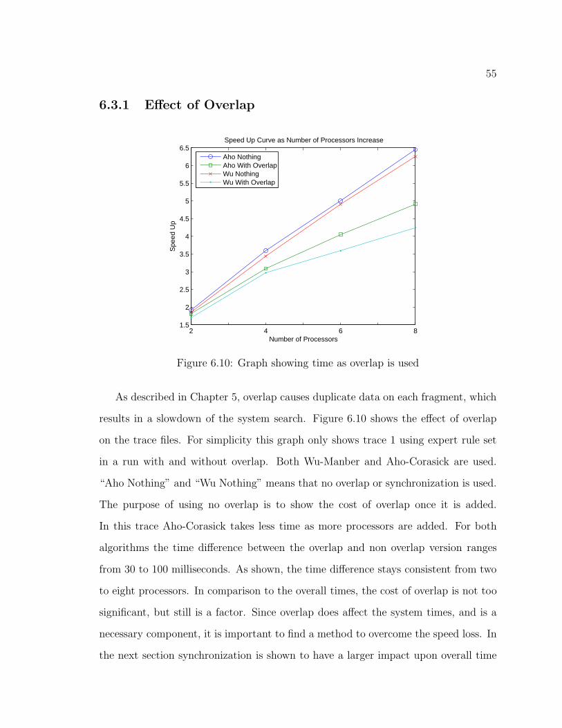
55

6.3.1 Effect of Overlap

2 4 6 81.5

2

2.5

3

3.5

4

4.5

5

5.5

6

6.5


Spe

ed U

p


Aho NothingAho With OverlapWu NothingWu With Overlap

Figure 6.10: Graph showing time as overlap is used

As described in Chapter 5, overlap causes duplicate data on each fragment, which

results in a slowdown of the system search. Figure 6.10 shows the effect of overlap

on the trace files. For simplicity this graph only shows trace 1 using expert rule set

in a run with and without overlap. Both Wu-Manber and Aho-Corasick are used.

“Aho Nothing” and “Wu Nothing” means that no overlap or synchronization is used.

The purpose of using no overlap is to show the cost of overlap once it is added.

In this trace Aho-Corasick takes less time as more processors are added. For both

algorithms the time difference between the overlap and non overlap version ranges

from 30 to 100 milliseconds. As shown, the time difference stays consistent from two

to eight processors. In comparison to the overall times, the cost of overlap is not too

significant, but still is a factor. Since overlap does affect the system times, and is a

necessary component, it is important to find a method to overcome the speed loss. In

the next section synchronization is shown to have a larger impact upon overall time

56

2 4 6 80

2

4

6

8

10

12

14


Spe

ed U

p


Aho NothingAho With SynchronizationWu NothingWu With Synchronization

Figure 6.11: Graph showing time as synchronization is used

reduction.

6.3.2 Effect of Synchronization

The same method of synchronization that is explained in Chapter 5 is used for DDP.

This section evaluates the cost of using synchronization. For simplicity only trace 1

using the expert rule set is used in Figure 6.11 with both the Wu-Manber and Aho-

Corasick algorithms. The figure shows that synchronization significantly reduces the

overall time as more processors are added. In this graph Aho-Corasick outperforms

Wu-Manber when synchronization is used and when synchronization is not used. The

speed gain in this graph ranges from 100 to 250 milliseconds.

6.3.3 DDP Results

For the previous two subsections, graphs were shown that outline the performance of

adding overlap and synchronization to the DDP method. According to the synchro-

57

nization results it is apparent that the synchronization component needs to be added

to the system. It is needed because synchronization will overcome the cost of adding

overlap. The overlap slows the system down, and if possible it would be removed.

The overlap however insures the integrity of the system, and is therefore a necessary

component.

2 4 6 80

2

4

6

8

10

12

14


Spe

ed U

p


Aho NothingAho With OverlapAho With SynchroWu NothingWu With OverlapWu With Synchro

Figure 6.12: speedup of all variations of DDP

In Figure 6.12 a speedup graph of all combinations using Aho-Corasick on trace

1 with the expert rule set of overlap and synchronization is shown. The combination

of synchronization without overlap performs the best in this system, because it has

the benefit of the speed gains from synchronization, but does not have the reduction

of speed using overlap. However this version should not be implemented because it

lacks system integrity. The next best option is the current DDP system using both

synchronization and overlap. Upon looking at the graph there is a clear separation

between the versions that use synchronization and those that do not. There is a small

separation when overlap is added in the negative direction. This trend continues

58

throughout all traces and indicates that synchronization has a larger effect on the

data than overlap.

1 2 4 6 81

2

3

4

5

6

7

8

9

10

11


Spe

ed U

p


DP AhoDDP AhoDDP WuDP WuDP Dual

Figure 6.13: speedup curve of all algorithms

Figure 6.13 shows that the DDP method has the best two times using Aho-

Corasick and Wu-Manber respectively. In data parallel the Dual and Wu-Manber

algorithms mirror each other while the Aho-Corasick algorithm begins to slow as

more processors are added. The important thing to note in this graph is the large

speedup and scalability of the DDP method as more processors are added. Figure

6.14 is a graph of each algorithm’s time as processors are added. This graph shows a

few different trends with the data parallel approaches. Again, clearly the two DDP

methods show the largest decrease in time as more processors are added. In this graph

the Dual-Algorithm clearly performs better the other two data parallel methods. The

difference between these two graphs is that the speedup graph shows the scalability

of the algorithms, and the time shows the best algorithm for the given number of

processors. In both graphs DDP using Aho-Corasick has been shown to have the best

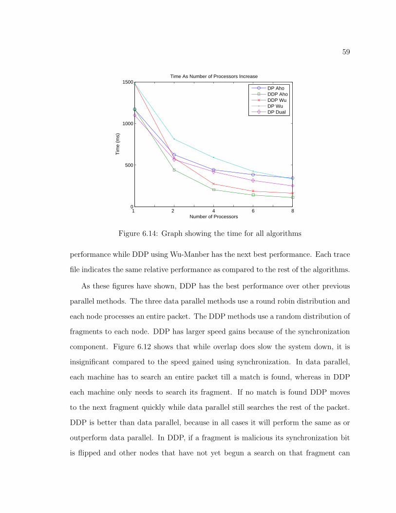
59

1 2 4 6 80

500

1000

1500


Tim

e (m

s)

Time As Number of Processors Increase

DP AhoDDP AhoDDP WuDP WuDP Dual

Figure 6.14: Graph showing the time for all algorithms

performance while DDP using Wu-Manber has the next best performance. Each trace

file indicates the same relative performance as compared to the rest of the algorithms.

As these figures have shown, DDP has the best performance over other previous

parallel methods. The three data parallel methods use a round robin distribution and

each node processes an entire packet. The DDP methods use a random distribution of

fragments to each node. DDP has larger speed gains because of the synchronization

component. Figure 6.12 shows that while overlap does slow the system down, it is

insignificant compared to the speed gained using synchronization. In data parallel,

each machine has to search an entire packet till a match is found, whereas in DDP

each machine only needs to search its fragment. If no match is found DDP moves

to the next fragment quickly while data parallel still searches the rest of the packet.

DDP is better than data parallel, because in all cases it will perform the same as or

outperform data parallel. In DDP, if a fragment is malicious its synchronization bit

is flipped and other nodes that have not yet begun a search on that fragment can

60

skip searching. These advancements over traditional data parallel approaches allow

the DDP method to have faster search times and a better overall speedup.

6.4 Wu-Manber with Excludes

Due to the nature of the Wu-Manber algorithm if the smallest rules can be omitted

a larger amount of data can be skipped if a match is not found. A rule of size one

severely limits the speed because only one byte can be skipped at a time. If there are

no rules below five then the Wu-Manber algorithm could skip five bytes at a time,

resulting in a theoretical speed gain of 5 times over rule sets with one byte rules.

The Aho-Corasick algorithm is affected by larger rules, but only when the rule set is

small in size. Since a typical IDS rule set is large, the finite state machine is rarely

affected by large rules unless they are incredibly substantial. Excluding small rules

from Aho-Corasick will not alter the speed of the algorithm.

This section will show the effect of excluding small rules from the rule set on the

DDP Wu-Manber algorithm. Exclusion simply means removal of those rules Figure

6.15 shows the normal Wu-Manber and Aho-Corasick algorithms, as well as the Wu-

Manber excluding rules of size (1, 2), (1, 2, 3), and (2, 3, 4).

Figure 6.15 uses trace 1 with the expert rule set and the DDP method for its

tests. The DDP Aho-Corasick and Wu-Manber results are the same as in the previous

sections. As shown, Aho-Corasick’s time is faster than Wu-Manber, however as certain

rules are excluded the Wu-Manber algorithm outperforms Aho-Corasick. When the

rules (1, 2) and (1, 2, 3) are excluded Wu-Manber performs better than Aho-Corasick.

The reason for this is when rules (1, 2) are excluded if no match is found the algorithm

can skip 3 bytes at a time. This reduces the sequential time from 1477 to 562, nearly a

3 times decrease in time. The same happens when rules (1, 2, 3) are excluded. When

rules (2, 3, 4) are excluded Wu-Manber only has minimal speed gains so that Aho-

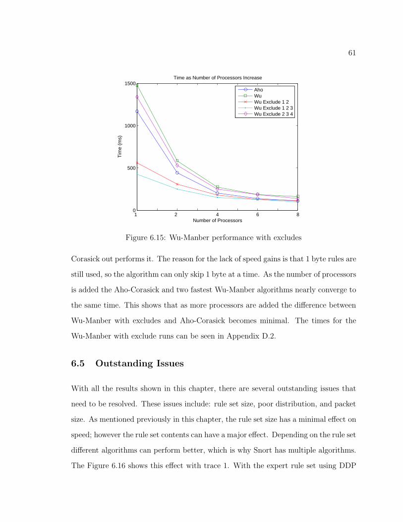
61

1 2 4 6 80

500

1000

1500


Tim

e (m

s)

Time as Number of Processors Increase

AhoWuWu Exclude 1 2Wu Exclude 1 2 3Wu Exclude 2 3 4

Figure 6.15: Wu-Manber performance with excludes

Corasick out performs it. The reason for the lack of speed gains is that 1 byte rules are

still used, so the algorithm can only skip 1 byte at a time. As the number of processors

is added the Aho-Corasick and two fastest Wu-Manber algorithms nearly converge to

the same time. This shows that as more processors are added the difference between

Wu-Manber with excludes and Aho-Corasick becomes minimal. The times for the

Wu-Manber with exclude runs can be seen in Appendix D.2.

6.5 Outstanding Issues

With all the results shown in this chapter, there are several outstanding issues that

need to be resolved. These issues include: rule set size, poor distribution, and packet

size. As mentioned previously in this chapter, the rule set size has a minimal effect on

speed; however the rule set contents can have a major effect. Depending on the rule set

different algorithms can perform better, which is why Snort has multiple algorithms.

The Figure 6.16 shows this effect with trace 1. With the expert rule set using DDP

62

and trace 1, Aho-Corasick outperformed Wu-Manber, but with the Snort rule set

this is not the case. Using the original rule set and DDP method the Wu-Manber

algorithm doubles the performance of Aho-Corasick. DDP using Aho-Corasick still

out performs data parallel using Wu-Manber with a rule set that is geared towards

the Wu-Manber algorithm. This example truly shows the power of the DDP method,

because even while using the wrong algorithm for the rule set, DDP outperforms data

parallel using the right algorithm for the rule set. Rule sets are important, but they

affect the searching algorithm and not the parallel techniques.

1 2 4 6 81

2

3

4

5

6

7

8

9

10

11


Spe

ed U

p


DP AhoDDP AhoDDP WuDP Wu

Figure 6.16: Graph showing difference between rule sets

Even with changing rule sets the DDP method continues to show that it is more

powerful than any other parallel method. One problem that could occur in a parallel

approach is poor distribution of packets. In data parallel the packets are distributed

in a round robin fashion and if uniform data is entering at the same distribution

rate, similar probability packets can be sent to the same node. If one node has the

same style of packets, then those packets will most likely have similar content. The

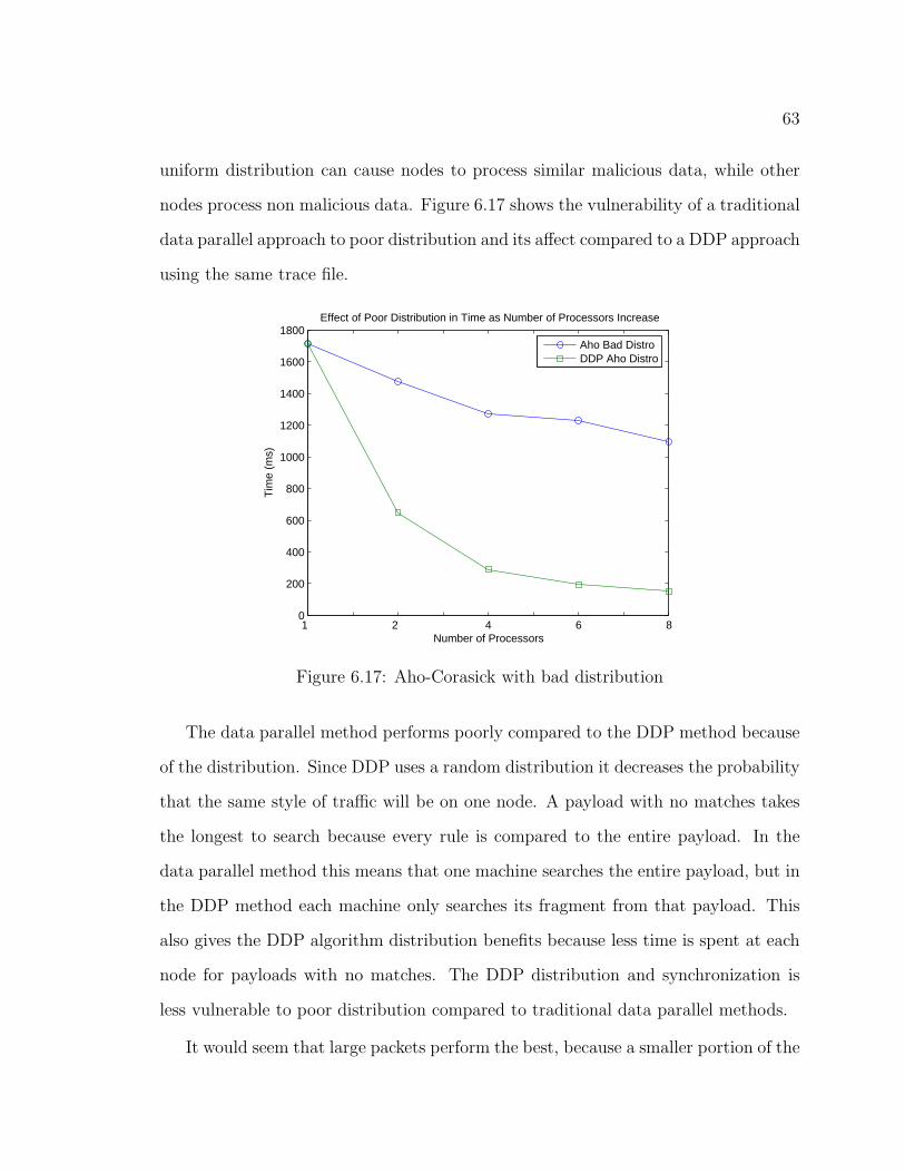
63

uniform distribution can cause nodes to process similar malicious data, while other

nodes process non malicious data. Figure 6.17 shows the vulnerability of a traditional

data parallel approach to poor distribution and its affect compared to a DDP approach

using the same trace file.

1 2 4 6 80

200

400

600

800

1000

1200

1400

1600

1800


Tim

e (m

s)

Effect of Poor Distribution in Time as Number of Processors Increase

Aho Bad DistroDDP Aho Distro

Figure 6.17: Aho-Corasick with bad distribution

The data parallel method performs poorly compared to the DDP method because

of the distribution. Since DDP uses a random distribution it decreases the probability

that the same style of traffic will be on one node. A payload with no matches takes

the longest to search because every rule is compared to the entire payload. In the

data parallel method this means that one machine searches the entire payload, but in

the DDP method each machine only searches its fragment from that payload. This

also gives the DDP algorithm distribution benefits because less time is spent at each

node for payloads with no matches. The DDP distribution and synchronization is

less vulnerable to poor distribution compared to traditional data parallel methods.

It would seem that large packets perform the best, because a smaller portion of the

64

packet is overlap, whereas small packets perform worst because they contain a larger

portion of overlap. The results however show otherwise, and one main reason is the

distribution algorithm. Very small packets cannot be split, so the random distribution

sends them quickly to different nodes. For this system the largest pattern length was

80, and packet sizes of 1360, 680, 340, 170, and 85 were tested. These sizes were

chosen so an even packet size value was used. Figure 6.18(a) below shows the total

amount of data that needs to be processed per group of processors. It is computed

as:

(psize+(n−1)∗(mpat−1))∗x = data

psize = size of each packetn = number of nodes used in the systemmpat = length of the maximum patternx = number of packets sent through system

For each doubling packet size the number of packets used is halved. The reason for

this is to maintain the same amount of data throughout the system, because doubling

the data will obviously lead to increased times. The trace files used were worse case

traces that used the same data with no malicious pattern matches. The packet size

85 performed the best, whereas the packet size 1360 performed the second best. The

packet size 85 performed the best because it required no overlap. The packet size of

1360 performed the second best because it had the lowest number of overlapped data,

which resulted in the second lowest number of bytes processed through the system.

The Figure 6.18(b) is a graph of the times as the packet size changes and Figure

6.18(a) the number of bytes sent through the system. Taking this into account, DDP

is able to handle all TCP packet sizes without major variations in speed.

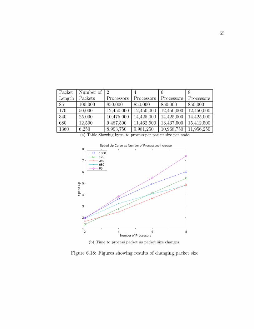
65

Packet Number of 2 4 6 8Length Packets Processors Processors Processors Processors85 100,000 850,000 850,000 850,000 850,000170 50,000 12,450,000 12,450,000 12,450,000 12,450,000340 25,000 10,475,000 14,425,000 14,425,000 14,425,000680 12,500 9,487,500 11,462,500 13,437,500 15,412,5001360 6,250 8,993,750 9,981,250 10,968,750 11,956,250

(a) Table Showing bytes to process per packet size per node

2 4 6 81

2

3

4

5

6

7

8


Spe

ed U

p


136017034068085

(b) Time to process packet as packet size changes

Figure 6.18: Figures showing results of changing packet size

Chapter 7: Conclusions and Future Work

As network line speeds increase, so does the need for faster security measures.

One method to protect networks is to implement an intrusion detection system. IDS,

like Snort, have been traditionally used on slower networks with security needs. Snort

only guarantees support on a 100Mbps network without dropping any packets. Sev-

eral attempts have been made to increase the speed of an IDS by updating algorithms,

hardware, and parallelization. Most approaches attempt to reduce the content match-

ing time because up to 70% of the time is spent here.

Several methods created in this paper have shown to increase the speed of an

IDS so that it can support high speed networks. Several improvements have been

created, including algorithms within Snort itself. Snort optimized its algorithms so

that they are tuned to an IDS. Several other algorithms were introduced such as

Pirahna, Ex2b, and Dual. Of these algorithms Dual showed the most promise for

support of increasing line speeds.

Several parallel methods were discussed including function and data parallel. The

function parallel approach of spreading Wu-Manber hash tables across nodes, showed

limited speed gains. The data parallel methods however, showed increased speed

gains to support high speed networks. The data parallel method distributed packets

using a round robin splitter to each node in the system. The data parallel method

can use any search algorithm, and was tested with Wu-Manber, Aho-Corasick, and

Dual-Algorithm. Of these three, Wu-Manber and Dual-Algorithm showed similar

performance, while the Aho-Corasick algorithm had limited performance. This paper

improved upon past parallel techniques and introduced a new method called Divided

66

67

Data Parallel.

The DDP method is a new method of dividing each packet into fragments and

distributing those packets to all nodes, while using synchronization. Past research has

used this method without clear results and without the synchronization component.

The DDP method uses packet overlap to avoid false negatives and uses synchroniza-

tion for increased speed gains. This paper has shown that DDP has speed gains

greater than any other parallel method. Like other data parallel methods, DDP can

support multiple algorithms. The Aho-Corasick and Wu-Manber algorithm were used

to test DDP, with Aho-Corasick performing better on expert rule sets.

Several issues were brought up including rule set size, poor duplication, and packet

size. When the rule set changes the content matching algorithms structures also

change. This paper showed that even when DDP uses the worst performance algo-

rithm; it outperforms previous parallel methods that are using the best performance

algorithm. The DDP algorithm is shown to be less susceptible to poor duplication,

because of the random distribution and the nature of fragmenting. Packet size is not

a major factor, because each fragment is broken and synchronization helps offset the

extra work caused by overlap.

Even with all the experiments in this paper, there are potential possibilities for

future work. The method of function parallel in this paper underperformed. There

are other methods mentioned that were not tested. Future work could include using

a function parallel system that breaks rules based on protocols. Further, a hybrid

system could be implemented that uses the function parallel distribution of protocols

to each machine that uses DDP on its nodes.

This paper introduced the DDP method and showed speed gains during the con-

tent matching phase. Future work could implement the entire system on a real net-

work, and analyze the cost of dividing packets on total system speed. The system

68

would need a method of random packet generation for high speed networks, and a

packet splitter.

Other future work could include different algorithmic approaches in use with DDP.

The Dual-Algorithm showed promise on a data parallel system so it could be imple-

mented in the DDP system. Other ways of choosing the content value to match on

could be researched. In the current system, the largest content word is picked for the

initial search to match on. Piranha[2] introduced a way to choose the rarest content

word to match on. Work could use the rarest content word and see how that alters

any other algorithm and the DDP system.

References

[1] Alfred V. Aho and Margaret J. Corasick. Efficient string matching: An aid tobibliographic search. Communications of the ACM, 18(6), June 1975.

[2] Antonatos Polychronakis Akritidis. Piranha: A fast lookup pattern matchingalgorithm for intrusion detection.

[3] Julia Allen, Alan Christie, William Fithen, John McHugh, Jed Pickel, andEd Stoner. State of the practice of intrusion detection technologies. Techni-cal report, Carnegie Mellon Software Engineering Institute, January 2000.

[4] K.G. Anagnostakis, S. Antonatos, E. P. Markatos, and M. Polchronakis. e2xb: Adomain-specific string matching algorithm for intrusion detection. In 18th IFIPInternational Information Security Conference, 2003.

[5] S. Antonatos K.G. Anagnostakis and E. P. Markatos. Generating realistic work-loads for network intrusion detection systems. In Proceedings ACM Workshopon Software and Performace., 2004.

[6] Herbert Boss and Kaiming Huang. A network intrusion detection sys-tem on ixp1200 network processors with support for large rule sets.http://citeseer.csail.mit.edu/703003.html.

[7] Robert S. Boyer and J. Strother Moore. A fast string searching algorithm. Com-munications of the ACM, 20(10):762–772, 1977.

[8] Richard Cole. Tight bounds on the complexity of the boyer-moore string match-ing algorithm. Symposium on Discrete Algorithms, pages 224–233, 1991.

[9] Symantec Corp. Symantec manhunt, 2004.

[10] Juan M. Estevez-Tapiador Pedro Garcia-Teodoro Jesus E. Diaz-Verdejo.Stochastic protocol modeling for anomaly based network intrusion detection.2003.

[11] Errin W. Fulp. Parallel firewall designs for high-speed networks. IEEE INFO-COM, High Speed Networking Workshop, 2006.

[12] R. Nigel Horspool. Practical fast searching in strings. Software-Practice andExperience, 10:501–506, 1980.

[13] Toby Kohlenberg. Snort IDS and IPS Toolkit. Syngress Publishing Inc., 2007.

69

70

[14] Stephen Northcutt and Judy Novak. Network Intrusion Detection. New RidersPublishing, 2003.

[15] E.P. Markatos S. Antonatos M. Polychronakis and K.G. Anagnostakis. Exb:Exclusion-based signature matching for intrusion detection. In IASTED Inter-national Conference on Communications and Computer Networks (CCN), page146152, November 2002.

[16] Snort. Snort - the de facto standard for intrusion detection/prevention.http://www.snort.org.

[17] Sourcefire. Sourcefire network security. http://www.sourcefire.com/.

[18] Sourcefire. Snort Users Manual, December 2006.

[19] Eugene Spafford and Diego Zamboni. Data collection mechanisms for intrusiondetection systems. CERIAS Technical Report 2000-08, CERIAS, Purdue Uni-versity, June 2000.

[20] S. Staniford-Chen, S. Cheung, R. Crawford, M. Dilger, J. Frank, J. Hoagland,K. Levitt, C. Wee, R. Yip, and D. Zerkle. GrIDS – A graph-based intrusiondetection system for large networks. In Proceedings of the 19th National Infor-mation Systems Security Conference, 1996.

[21] CERT. CERT/CC statistics 1988-2006. http://www.cert.org/stats.

[22] Bleeding Edge Threats. Bleeding edge threats.http://www.bleedingthreats.net.

[23] Giovanni Vigna, Fredrik Valeur, and Richard A. Kemmerer. Designing and im-plementing a family of intrusion detection systems. ACM SIGSOFT SoftwareEngineering Notes, 28(5):88–97, September 2003.

[24] Chi-Ho Tsang Sam Kwong Hanli Wang. Anomaly intrusion detection usingmulti-objective genetic fuzzy system and agent-based evolutionary computationframework. 2005.

[25] Patrick Wheeler and Errin W. Fulp. A taxonomy of parallel techniques forintrusion detection. ACMSE 2007, 2007.

[26] Patrick Stuart Wheeler. Techniques for improving the performance of signa-ture based intrusion detection systems. Master’s thesis, University of CaliforniaDavis, 2006.

[27] Sun Wu and Udi Manber. A fast algorithm for multi-pattern searching. Technicalreport, University of Arizona, May 1994.

71

[28] Jianming Yu and Jun Li. A parallel nids pattern matching engine and its imple-mentation on network processor. In 2005 International Conference on Securityand Management (SAM 2005), 2005.

[29] Mohammad Al-Subaie Mohammad Zulkernine. Efficacy of hidden markov mod-els over neural networks in anomaly intrusion detection. 2006.

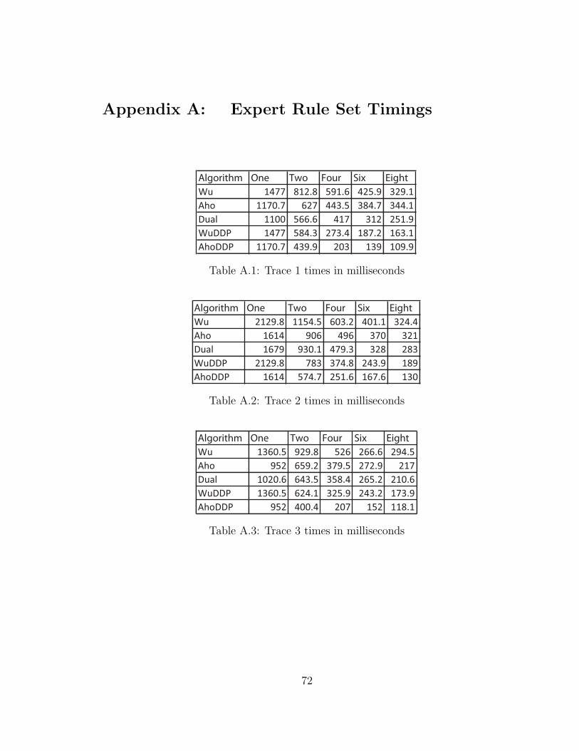
Appendix A: Expert Rule Set Timings

Algorithm One Two Four Six Eight

Wu 1477 812.8 591.6 425.9 329.1

Aho 1170.7 627 443.5 384.7 344.1

Dual 1100 566.6 417 312 251.9

WuDDP 1477 584.3 273.4 187.2 163.1

AhoDDP 1170.7 439.9 203 139 109.9

Table A.1: Trace 1 times in milliseconds


Wu 2129.8 1154.5 603.2 401.1 324.4

Aho 1614 906 496 370 321

Dual 1679 930.1 479.3 328 283

WuDDP 2129.8 783 374.8 243.9 189

AhoDDP 1614 574.7 251.6 167.6 130



Wu 1360.5 929.8 526 266.6 294.5

Aho 952 659.2 379.5 272.9 217

Dual 1020.6 643.5 358.4 265.2 210.6

WuDDP 1360.5 624.1 325.9 243.2 173.9

AhoDDP 952 400.4 207 152 118.1


72

73


Wu 601.2 310 163.6 115 89.7

Aho 482.1 250 154 112.2 97

Dual 449.1 233 125.9 90.3 78.1

WuDDP 601.2 230 115.1 77 60.1

AhoDDP 482.1 180.3 80.2 56.2 45



Wu 1066 593.6 289.7 201 160

Aho 823 436.1 223 154 128.5

Dual 653 345 181 123.6 103.6

WuDDP 1066 406.2 180 123.1 98

AhoDDP 823 300.3 135.1 92 74.1



Wu 1595.6 955.2 554.7 425.1 424.9

Aho 1131.3 721.6 381 337.7 288.6

Dual 1262.8 742.9 415 324.7 303.5

WuDDP 1595.6 691.7 353 226.1 193.2

AhoDDP 1131.6 449 208.3 142 111.6


Appendix B: Snort Rule Set Timings


Wu 2504 1369.8 914.4 677.2 610.8

Aho 2482.8 1409 1021 886.8 902.2

Dual 3282.6 1636.8 1193.6 946.8 447.8

WuDDP 2504 946.8 447.8 297.8 234.6

AhoDDP 2482.8 1349.8 785.2 575.4 499.8

Table B.1: Trace 1 times in milliseconds


Wu 4142 2423.2 1300.6 971.4 786.6

Aho 4245 2564.4 1345.6 1014.8 1041.4

Dual 5153 2857.8 1447.2 974.8 836.6

WuDDP 4142 1505.6 721.4 481.6 350

AhoDDP 4245 2297.4 1296.2 968.6 832.2



Wu 2527.8 1494 774 554 440.2

Aho 2056 1181.4 637.6 466.2 389.4

Dual 3260 1927.4 1037 736 604.8

WuDDP 2527.8 1156 556.4 405.6 305.6

AhoDDP 2056 1190 710.2 544 435.4


74

75


Wu 994.4 545 310 208 192

Aho 1021 541 347 274.2 286

Dual 1317 658 364 248 202

WuDDP 994.4 401.8 174 117.8 91.2

AhoDDP 1021 555.8 320.2 242.4 219.8



Wu 1559.4 874 450 339.8 240.2

Aho 1480 817.2 433.8 308.4 274

Dual 2197.6 1172.6 588.2 406.6 319

WuDDP 1559.4 572.4 266 178.2 135

AhoDDP 1480 804.8 464.2 355 299.4



Wu 3394 2067.2 1112 777 758.2

Aho 2957 1825.8 928.6 850.2 734.4

Dual 4089.89 2358.4 1284 958 898.6

WuDDP 3394 1419.8 746.8 479.2 369.8

AhoDDP 2957 1663.8 925.6 686 576


Appendix C: DDP Rule Set Variations

Algorithm Two Four Six Eight

DDP Wu Nothing 790.2 428.6 300.4 236

DDP Aho Nothing 607.2 324.8 234 181.4

DDP Wu with Overlap 865.2 497 410.4 347

DDP Aho with Overlap 645.2 378.2 289 238

DDP Wu with Synchro 551 238.4 156 117

DDP Aho with Synchro 410.8 174 116 87

Table C.1: Trace 1 times in milliseconds


DDP Wu Nothing 1142 594 461.2 326.4

DDP Aho Nothing 831 436 302 241

DDP Wu with Overlap 1181.2 749.6 524.2 441

DDP Aho with Overlap 893.2 515.6 385.2 325

DDP Wu with Synchro 752.8 311.6 210.8 146.2

DDP Aho with Synchro 539 217.8 137 101.8



DDP Wu Nothing 750 444.2 294 226

DDP Aho Nothing 513.8 283 204.6 160

DDP Wu with Overlap 866.6 519 454.2 364

DDP Aho with Overlap 561 357 290.4 229.6

DDP Wu with Synchro 550 270 175.2 134

DDP Aho with Synchro 367 170.2 117 91


76

77


DDP Wu Nothing 334 182 134 104


DDP Wu with Overlap 352 215 168 130.6

DDP Aho with Overlap 267 157.2 121 102

DDP Wu with Synchro 224 98 66 49

DDP Aho with Synchro 168.6 70 46 35.8



DDP Wu Nothing 574.4 307.2 213 185


DDP Wu with Overlap 594 369 282.8 226

DDP Aho with Overlap 450 264.4 204 171

DDP Wu with Synchro 379.6 159.2 102 82

DDP Aho with Synchro 281 118.6 76.8 58



DDP Wu Nothing 896.4 463 323 285

DDP Aho Nothing 598.6 312 223.2 172

DDP Wu with Overlap 929.2 534 437 352

DDP Aho with Overlap 646.4 366 279 231

DDP Wu with Synchro 665.2 291.2 190 161

DDP Aho with Synchro 416 181.6 118 89


Appendix D: Other Timings

D.1 Function Parallel

Trace Algorithm Two Four Six Eight

Trace1 FP 1419.8 1441.8 1383 1400.6

Trace3 FP 1372.4 1372.8 1335.6 1334.4

Trace4 FP 569 567 553 550.6

Table D.1: Time for traces in milliseconds

D.2 Wu-Manber Excludes

Algorithm Excludes One Two Four Six Eight

WuDDP 1 2 559.2 307.2 179 144 112.1

WuDDP 1 2 3 426.1 233.8 150.8 109 113

WuDDP 2 3 4 1320.6 543.6 249.5 187.8 138.7

Table D.2: Trace 1 times in milliseconds


WuDDP 1 2 853.1 381 207 152.4 129.2

WuDDP 1 2 3 600.8 286.5 156.3 121.2 109.6

WuDDP 2 3 4 1673 627.8 298.2 194.1 159.5



WuDDP 1 2 424.1 279 178.7 176 122

WuDDP 1 2 3 312.1 254 155 162.6 169

WuDDP 2 3 4 1169.1 541.8 271.1 198.3 154.1


78

79


WuDDP 1 2 235 119 66 51 55.6

WuDDP 1 2 3 176 92 54 43 45

WuDDP 2 3 4 534 217.9 103 76.1 61.1



WuDDP 1 2 306 177 114.4 88.2 87.6

WuDDP 1 2 3 221 135.4 93 81 70

WuDDP 2 3 4 1017 392.3 175.1 119 102



WuDDP 1 2 549.8 326.7 189.3 132 129.1

WuDDP 1 2 3 414 245.1 157.9 127 117

WuDDP 2 3 4 1256.9 572 264 199 144.1


Vita

Chris V. Kopek

• 5457 Hunt Club Drive, Virginia Beach VA, 23462email: [email protected]: (757)343-9178

Education

• Master of Science, Computer ScienceWake Forest University, Winston-Salem, NCMay, 2007Thesis: “Parallel Intrusion Detection Systems for High Speed Networks usingthe Divided Data Parallel Method”

• Bachelor of Science, Computer Science with Minor in TelecommunicationsJames Madison University, Harrisonburg, VAMay, 20053.5 GPA in Major3.4 GPA Overall

Publication

• “Managing Security Policies for High-Speed Function Parallel Firewalls.” ErrinW. Fulp. Micheal R. Horvath, and Chris Kopek. SPIE 3rd International Sym-posium on High Capacity Optical Networks and Enabling Technology, 2006.

• “Corporate wireless LAN security: threats and an effective security assessmentframework for wireless information assurance” Young B. Choi, Jeffrey Muller,Christopher V. Kopek, and Jennifer M. Makarsky. International Journal ofMobile Communications 2006 - Vol. 4, No.3 pp. 266 - 290.

• “Geographic Information System for Simulating Container Movement (GISSCM).”Helmut Kraenzle, Elizabeth Cahill, Matthew Chenault, Chris Kopek, MeganMcCarthy, and Amy Ozeki. Critical Infrastructure Protection Program Work-shop II Working Papers. Arlington, VA: George Mason University Press.

80

81

Experience

• Teachers AssistantWake Forest University, Winston-Salem, NCAugust 2005 – May 2007Assisted in teaching 2 different introductory Computer Science courses. Coursesrequired skills and knowledge with the following languages and pieces of soft-ware: Adobe Software Suite, Java, JavaScript, CSS, HTML, and Microsoft Ac-cess. Duties involved: teaching, answering questions, solving student problems(troubleshooting), and grading papers.

• ConsultantGreat Wall Systems, Winston-Salem, NCMay 2006 – August 2006Worked to form algorithms for parallelization of firewall rules. Played a keyrole in a team of 2 to form an algorithm to parallelize firewall rules for functionparallel firewalls. Research was funded from a Department of Energy (DOE)Grant

• ProgrammerJames Madison University, Harrisonburg, VAJanuary 2004 – September 2004Assisted in the development of two projects for the Spatial Information Clear-inghouse (SIC), at James Madison University. Extreme Programmer, for projectcalled Simulating Container Movement using Global Information Systems (SCMGIS),and main programmer for project called SIC. Duties for SCMGIS and SIC in-cluded programming, designing, and testing of software. For SCMGIS, thesoftware coded in VB .NET, simulated the movement of shipping containersaround the world, using real life routes, and data, obtained from port authority.For SIC the software was coded in HTML, JavaScript, and CSS, and was usedfor miners worldwide, for the location of land mines. For both projects I workedin a team of 6 to 8 people.

Honors

• Dean’s List Fall 2005.

• Event Organizer Upsilon Pi Epsilon 2007.

• NSTISSI No. 4011 Certification for Information Systems Security Professionals.

• 2nd place in NASA AMES competition for data mining/anomaly detection.

parallel intrusion detection systems for high speed

Documents