Purdue UniversityPurdue e-PubsDepartment of Computer Science TechnicalReports Department of Computer Science

1993

Parallel Electronic Prototyping of Physical ObjectsPoting Wu

Elias N. HoustisPurdue University, enh@cs.purdue.edu

Report Number:93-026

This document has been made available through Purdue e-Pubs, a service of the Purdue University Libraries. Please contact epubs@purdue.edu foradditional information.

Wu, Poting and Houstis, Elias N., "Parallel Electronic Prototyping of Physical Objects" (1993). Department of Computer ScienceTechnical Reports. Paper 1044.https://docs.lib.purdue.edu/cstech/1044

PARALLEL ELECTRONIC PROTOTYPINGOF PHYSICAL OBJECfS

Poting WuE. N. Roustis

CSD·TR·93·0Z6April 1993

Parallel Electronic Prototyping of Physical Objects

Poting Wu and Elias N. Houstis

Department of Computer SciencesPurdue University

West Lafayette, Indiana 47907, U.S.A.e-mail: wu@cs.purdue.edu

Technical Report CSD-TR-93-026CAPO Report CAPO-93-19

April, 1993

AbstractThe electronic prolotyping of a physical object starts with the user completelyspecifying the problem on an assumed initial geometry, followed by the simulationof the physics and the satisfiability of some a priori defined design objectives. Theprocess might be repeated several times until the optimal design is obtained. Thispaper addresses the various issues involved in the parallel implementation of theabove design process. The methodology adopted is applied on the continuous anddiscrete geometric data associated with the physical object and the simulation ofits physics respectively. In this paper we present the formulation of the parallelelectronic prototyping process for some class of structural engineering problemsand the parallel algorithms developed and implemented on the nCUBE II machinefor the realization of adaptive mesh generation, mesh splitting and shapeoptimization together with their measured performance.

This work was supported by NSF grants 9123502-CDA and 9202536·CCR, AFOSR F49620-92-]·0069 andPRF _'6902003.

- i -

CONTENTS

Chapter 1 Introduction

1.1 Geometry-based modeling subsystems1.2 Parallel mesh and mesh-splitting preprocessor1.3 Analysis and shape optimization

Chapter 2 Parallel Adaptive Mesh Generation and Decomposition

2.1 Methodology of the parallel mesh generation and mesh splitting2.2 Fonnulation and implementation of initial refinable background grid

2.2.1 Mesh generation scheme2.2.1.1 Decompose domain into quadtree data structure2.2.1.2 Element meshes generation2.2.1.3 Element meshes adjustment2.2.1.4 Adjacency lists

2.2.2 Special techniques in mesh generation2.2.2.1 Neighbor finding2.2.2.2 Polygon locating recognition

2.3 Initial domain splitting2.3.1 Group I: Neighborhood - Searching scheme

2.3.1.1 Algorithm I: Depth - First Search2.3.1.2 Algorithm 2: Breadth - First Search

2.3.2 Group II: Domain -Axis scheme2.3.2.1 Algorithm 3: Cartesian Axis Splitting2.3.2.2 Algorithm 4: Polar Axis Splitting2.3.2.3 Algorithm 5: Inertia Axis Splitting

2.3.3 Perfonnance in domain decomposition algorithm2.4 Subdomain boundary linking2.5 Final mesh generating2.6 Final domain splitting2.7 Fully automatic mesh adaptation2.8 Perfonnance in parallel mesh generation

2.8.1 Performance 1 - Engine rod head2.8.2 Perfonnance 2 - Torque arm

- II -

1

233

5

56779121415151718181819202025282930313233353536

Chapter 3 Parallel Shape Optimization

3.1 Fonnulation of parallel shape optimization process3.2 Model coordination method3.3 Goal coordination method3.4 Examples of parallel shape optimization

3.4.1 Example 1 - Parallel shape optimization with load case #13.4.2 Example 2 - Parallel shape optimization with load case #2

37

373840434344

Chapter 4 References

- iii -

45

1 Introduction

This report presents the fannulation and implementation of preprocessing and postprocessinggeometry based tools for achieving the para11elization of the overall design and analysis ofphysical objects. These tools are part of a generic software we are building for the electronicprototyping of geometry based physical objects [HOllS 92]. Figure 1.1 shows a conceptual view ofthe processes involved in the electronic prototyping system. The prototyping of a physical objectstans with the user completely specifying the problem on an assumed initial geometry. Next afully automatic parallel mesh and mesh-splitting preprocessor creates the parallel discrete datastructures on each processor for the generation of the local discrete analysis and optimizationequations. For the implementation of the shape optimization phase the mesh is fully flexible(parametrized) so that it can be adapted based on the processing results. The shape adaptation isimplemented. on the mesh-splitting already defined on the local (subdomain) and global(interface) data.

Analysis &( Prototype Preprocessing ..... ~ Postprocessing ILocal Optimization

Motkling

Giohol Optimization I

Figure 1.1: The analysis and design process of a physical object.

- [ -

1.1 Geometry-based modeling subsystemsThere are many types of geometry model representations: wireframe, surface, or solid modeling.In our system we have integrated two solid modeling systems: XXoX and PATRAN. Followingwe give a brief overview of the two geometry modeling systems.

XXoX:

PATRAN:

This is a solid modeling system which is based on the XoX geometry andgraphics libraries [XoXE 92J. [XoXR 92] with an X-window interactive userinterface supporting CSG type primitive operations [WU 93]. In the XXoXenvironment one can create 3-D primitives and 2-D outlines of cross-sections.manipulate the geometry by orienting, combining, cutting, and defonning theobjects. XXoX provides extremely powerful multiple user-interlaces, and theUNDO/REDO functions by using the higher level programming interface ofthe Motif widget in one integrated program. For example, the description of anengine pan in XXoX language is as follows:

cylinderl = cylinder(O,O.-O.52,I.56,I.04)cylinder2 = cylinder(O,O,-O.52,l.04.1.04)cylinder3 = cylinder(O,O,O,O.5,5.4)oo~l = bo~(-O.26,-O.52,l.04,O.52.1.04.6.6)

rod = rota1e(cylinderl-cylinder2,O,O,O,O,I,O,-90)rod = rod Ibod Itrnnsl:lle(scale(rod,1,O.5,O.5),O,O.8.16)rod = rod Itranslate(roLale(cylinder3,O,O,O,O,l,O,·90),2.6,O,8.16)

Figure 1.2: The description of an engine part in XXoX language.

This is an open-ended, general purpose, 3-D MCAE (Mechanical ComputerAided Engineering) software package that uses interactive graphics to linkengineering design, analysis and results evaluation functions. By its solidgeometry editor, we can create virtually any geomeuy or modify existinggeomeuy imported from other design system. This environment is described in[Pattafl 92].

·2·

1.2 Parallel mesh and mesh-splitting preprocessorThe mapping of computations to parallel machines can be realized at the various data structuresassociated with the computations. In the case of PDE (Partial Differential Equations) basedapplications we have selected to fannulate this problem at the discrete data structures of theunderlying computation [Chri 91]. In this paper we formulate and implement parallel mappingalgorithms on distributed memory machines including the nCUBE II and Intel iPSC/860. Theuniqueness of our parallel mapping scheme is the fact that it integrates the mesh splitting(decomposition) with the mesh generation. Thus the mesh generation and mesh-splittingpreprocessors are integrated into one that runs in parallel on the targeted machine. Severalalgorithmic alternatives are investigated for implementing the various parts of this preprocessorincluding suitable algorithms for mesh generation [Lohn 92] and mesh decomposition [Coo 91],[Lori 88]. Local and global mesh refinements are also supported with mesh smoothing and sideswapping. Optimal domain partitioning algorithms of the mesh data are considered [Sava 91].Figure 1.3 shows the methodology on which the parallel mesh and mesh decompositionpreprocessor is based. the example assumes a 2-D region and on a 4-processor machine.

1.3 Analysis and shape optimizationThe analysis and shape optimization is implemented using the domain decompositionmethodology which is based on the static parallel mesh and mesh-splitting described above. Thedomain decomposition solvers of the parallel ELLPACK system [Hous 92] are currently used forthe analysis. For the shape optimization problem we are developing two phase semi-optimalalgorithms based on the local and global mesh and decomposition data [Ding 86].

- 3 -

o 1. Arefinable backgroundgrid algorithm is selectedto fonn the initial grid.

2. A scheme to split the ini­tial grid into equal-sizedsubdomains is applied.

3. A linking routine toform the new subdomainboundaries is called.

4. The mesh algorithm instep 1 is applied to gener­ate a finer mesh in parallel.

5. An optimal mesh split­ting scheme to minimize thebisection width is applied ....

Figure 1.3: The methodology of the parallel mesh and mesh-decomposition preprocessor.

-4-

2 Parallel Adaptive Mesh Generation and DecompositionIn general, the requirement to generate finite element meshes has been an obstacle of using thefinite-element method. However, there are many methods available today to assist in thegeneration of finite-element meshes. This is not to say that the generation of the element meshes isno longer a major bottleneck, but the situation today is better than it was. The need to generateelement meshes fast is common to a number of computational fields especially in adaptive finiteelement processor. Therefore, the mapping of element meshes generation to parallel machinesbecomes urgent. In this paper we fannulate and implement parallel mapping algorithms ondistributed memory machines including the nCUBE II and Intel iPSe/860. The uniqueness of ourparallel mapping scheme is the fact that it integrates the mesh splitting (decomposition) with themesh generation. Thus the mesh generation and mesh-splitting preprocessors are integrated intoone that runs in parallel on the targeted machine. Several algorithmic alternatives are investigatedfor implementing the various pans of this preprocessor including suitable algorithms for meshgeneration [Lohn 92] and mesh decomposition [Coo 91], [Lori 88]. Local and global meshrefinements are also supported with mesh smoothing and side swapping. Optimal domainpartitioning algorithms of the mesh data are considered [Sava 91].

2.1 Methodology of the parallel mesh generation and mesh splittingThe parallel mapping scheme in this article contains five major steps:

1. Fonn an initial refinahle backgroond grid:Algorithm is selected to form the initial grid. Because a fairly fine initial background gridcan be assumed which allows division of the background grid into subdomains of nearlyequal size with maximum difference of one. In the further step, we can use the samealgorithm and same code to generate mesh on subdomains in a parallel manner. Theseinclude the mesh generator, mesh refiner, mesh smoother, and mesh side swapper.

2. Split the initial grid into equal-sized subdomains:Several decomposition schemes are supponed so that for different shapes of geometryobjects we have the opportunity to test which algorithm is most optimal. In addition, thereis a "local optimal" scheme has been developed. This scheme makes decision on local datato split domain into two subdomains with minimum inter-node communication duringeach step of the domain decomposition.

3. Link the subdomains to fonn new boundaries:Before parallel mesh generation, we need to form the new boundary of the subdomainswhich we got from the domain decomposition phase. Since multi-region and new holesmay be created, extra effort will need in mesh generation and polygon locating recognitionalgorithm.

4. Generate finer element mesh in parallel:Since the introduction of the quadtree node distribution data structure, we can get therefined node distribution before generating mesh in parallel. Therefore, it will reduce thecommunication between the processor nodes to minimum. Furthermore, the generatedmesh will contain more global smoothness than other approach.

- 5 -

5. Minimize the bisection width between each subdomain:In practical, different sized sets of mesh with large number of edges between thesesubdomains may happen even we generated perfectly initial domain partition. Since thegoal of the optimal partition is NP-complete, in this step our algorithm will try to fonn anapproximately optimal graph partition instead.

2.2 Formulation and implementation of initial refinable background grid

The methods for the element meshes generation of unstructured grids can be classified into twofamilies:

1. Advancing front algorithms.2. Quadtree I Octree algorithms.

Several automatic mesh adaptation techniques on the first family of methods are found inprevious literatures. The scheme described in [Khan 91] can make the adaptation by predefinedthe node distribution on boundary only. Adaptation in [Lo 91] introduced the boundary andinternal contours to decide the node distribution when generating element meshes. Article of[Bykat 76] made adaptation possible by subdivision of a general polygon into convex subregions.All methods based on the advancing front algorithms can make mesh adaptation only on specifiedor computed boundary. And generate other internal element meshes by non-adaptive scheme orinterpolating computation.

The second family of methods are based on modifying an existing grid. The adaptation techniquein [Cheng 89] is defined on the user specified level assignment and vertex assignment.

For the automation and generality purpose, it seems appropriate to pursue the use of the quadtreeloctree algorithms for the following reasons:

1. Automation: Unlike the advancing front algorithms which users need to specified the nodedistributing information on objects boundary, the quadtree can automatically divides thedomain into a tree structure that depends on the objects geometry. Its critical state is tomaintain all the subregions be simple - each contains only one polygon venex or onepolygon segment.

2. Smoothness: Because the quadtree maintains the adjacency density to be 1/2 ratio ­difference of tree level between neighbors [Samet 82, 85, 89] is always no larger than one,it manages the adaptive node distribution not only on the outer boundary of objects butalso the internal region of objects. Therefore, it provides a global smooth node distributionwhen generating element meshes.

3. Adaptation: It is normal to refine whole domain globally or subregion locally. That is, itsupports a totally controlled tree structure that decides the node distribution. Therefore,adaptive finite element processor is easy and user specified refine region is possible.

4. Parallelism: Because the refining property, it has the information of the global nodedistribution before generating element meshes in paraJlel. This character can reduce thecommunication between processor nodes to minimum even zero.

·6-

2.2.1 Mesh generation scheme

2.2.1.1 Decompose domain into quadtree data structureThe introduction of quadtree in [Samet 84] defines the node distribution on its related hierarchicaldata structure. The following steps will call when 1. Create the initial background quadtree. and 2.Maintain a local or global refinement.

Stepl: Automatically divide the domain into a tree structure that depends on the objectsgeometry. Example in figure 2.1 shows that each subregion of quadtree should containonly one polygon vertex or one polygon segment after constructing the quadtreestructure. To achieve this simple criterion, it needs two basic geometric techniques ofthe vertices finding and line segment locating.

•

Figure 2.1: Construct quadtree structure on polygon object.

During constructing the quadtree structure. it also needs the tree level control toprevent the infinite refinement which occurred on few abnonnal shape as shown infigure 2.2.

2 polygon segments are 100 close

Figure 2.2: Infinite refinement occurred in abnonnal polygon.

·7·

Step2: Maintain the adjacency density to be 1/2 ratio as shown in the first quadrant of figure2.3. The neighbor finding techniques include face adjacency elements finding andcorner adjacency elements finding which will be described in sec. 2.2.2.1.

•>••••••••••••••••••••••••••••••••• ~ •••••••

I !Figure 2.3: Maintain the adjacency density to be If2 ratio.

Step3: Merge the alias nodes which have the same position but belong to different nodes inthe quadtree structure. It happens when vertex exactly locating on the quadtreedivision boundary like the case happens in figure 2.4. The reasons to merge them are togroup the element meshes in next phase easily and let the mesh smoothing and sideswapping work correctly.

..... /. ...

Figure 2.4: Merge the alias nodes.

·8·

2.2.1.2 Element meshes generationIn this stage, triangular element meshes will be generated by connecting the precomputed nodesin previous phase. The generating steps are as follows:

Stepl: Neighbor node finding and connecting - It includes three types of neighborconnecting:

1. NI-Nz or E1-E2 connections: When the northern neighbor or the eastern neighborexist and is not the leaf node of quadtree.

~E, .

/ E,\

Figure 2.5: Generate mesh by NI-NZ or E1-EZ connections.

2. E-N connection: When northern neighbor of the eastern neighbor is equal to thenorthern neighbor, or eastern neighbor of the northern neighbor is equal to theeastern neighbor.

•

Figure 2.6: Generate mesh by E-N connection.

3. E-NE-N connection: Happened when both cases in 2 are failed.

•Figure 2.7: Generate mesh by E-NE-N connection.

-9-

Step2: Divide quadrangle into tWO triangles - In E-NE-N connection, it selects the diagonalby following three criteria:

1. Common edge: Choose the diagonal which does not share a common edge toprevent an invalid zero area triangle created.

-------------

Figure 2.8: Choose the diagonal not share a common edge.

2. Overlapped ttiangular elements: Avoid to select the diagonal which will cause twocreated ttiangular elements be overlapped. This can be done by checking thecrossing point of these two diagonal.

------------------

Figure 2.9: Avoid to create overlapped triangular elements.

3. Shorter diagonal and Nearer area: Select the shorter diagonal which creates twotriangular elementS with the nearer area. (apply 2 factors on these two criteria.[Sadek 80D

ASFactor = Cd·=+C"

CD

(l!.. ACD) / (.6. BDC)

(.6. COAl/(l!.. DAB)

D

=C .AB+ C . ACUBOd CD "CO/DO

a,\

\, ...""..'0\

."...."" ,A ..•••···•••····•····.. ···....·....···•· "\

"""------1 c

Figure 2.10: Select shorter diagonal with nearer area.

- 10-

Step3: Triangle dividing - It needs to divide a triangular element if:

1. Vertex inside the triangular area: It needs to divide the original triangular elementinto three new triangular elements as following:

,,,,

,,,........'ll" ......

.......... ... ... , ...,~............

Figure 2.11: Vertex inside the triangular area.

2. Vertex on the triangular edge: It needs to divide the original triangular element intotwo new triangular elements recursively as following:

,,,

/ 151

Figure 2.12: Vertex on the triangular edge.

Step4: Triangle validating - A valid triangular element should be:

1. All three vertices are not outside polygon.2. Triangular area is larger than O.3. Centre of mass is inside polygon.

Step5: Triangle adjusting - We can apply on-line mesh smoothing and side swapping in thisstep locally. And after all meshes generated, apply them off-line globally again. Thesetwo techniques will discuss in next section.

In step 3 and 4, the polygon locating recognitioll technique is needed. It recognizes a vertex whereit located. That is, a vertex is inside, outside, on the edge, or on the vertices of the object polygon.It also needs to identify holes in the polygon. The detail of this technique will be described in sec.2.2.2.2.

• 11 •

2.2.1.3 Element meshes adjustmentPractical implementations of element meshes generation indicate that in certain region of themesh abrupt in element size of shape may be present. The usual way to solve this problem is toadjust the element and node distribution. This adjustment includes mesh smoothing and sideswapping.

1. Mesh smoothing. Here we introduce two adjust schemes to improve the unifonnity ofthe meshes. Since we have to know the adjacency nodes of current node to peIfonn thesmoothing, maintain a Node-node adjacency list is necessary when generating mesh:

a. Centre of mass - In each node smoothing, the standard Laplacian smoother isemployed. Each edge of triangular element is assumed to represent a spring.Therefore, we have the active force on the current node by:

"F = K· L (Xi-X)

;= I

where K denotes the spring factor. At the smoothing adjustment, we set F = 0 to get thecentre of mass as follows:

"

N2~----~>/N3

Figure 2.13: Mesh smoothing by the centre of mass.

b. Equilateral triangle - Instead of using adjacency nodes, we compute the equilateraltriangles from these nodes. And apply the same Laplacian smoothing scheme on thecurrent node by using the computed triangle nodes.

"

Figure 2.14: Mesh smoothing by the equilateral triangle.

- 12·

2. Side swapping ~ In this adjustment, each quadrilateral area which contains two triangularelements has been checked. We divide the current quadrilateral area into two newtriangular elements if they do not disobey the following two restrictions we discussed instep2 of sec. 2.2.1.2:a. Diagonal does not share a common edge.b. Diagonal does not create two overlapped triangular elements.

and these two new triangular elements will form a better diagonal factor for shorterdiagonal and nearer area we discussed:

_.-.

~-----2:YN3

Figure 2.15: Diagonal factor for side swapping.

• 13 •

2.2.1.4 Adjacency listsIn this implementation, four types of adjacency list are introduced: [Delj 90]

1. Node-node adjacency: It is a list of all the nodes adjacent to current node. We need itwhen mesh smoothing.

2. Node-element adjacency: It is constructed when node-node adjacency list is created. Weuse it when applied the side swapping.

In practical, we can combine these two list in one data structure as follows:

NS

NIE,

EI N,E,

E,

N2 N)

Figure 2.16: Structure for node-node & node~element adjacency list

3. Element-node adjacency: It contains three pointers to the three nodes for each triangularelement. It is the basic information for a mesh element

4. Element-element adjacency: It is constructed when node-element and element-nodeadjacency list are created. It is useful when calling neighborhood searching indecomposition process.

We can also connect these two adjacency list in one data structure as follows:

N,

Et

E

N,Nt

E,

Figure 2.17: Structure for element-node & element-element adjacency list.

Since all adjacency lists are constructed in the process of mesh generation, no expensivesearching process is needed. We use the information of these lists during mesh splitting andlinking processes.

- 14-

2.2.2 Special techniques in mesh generation

2.2.2.1 Neighbor findingNeighbor finding [Samet 82, 85, 89] includes two types of schemes in 2-D domain: one is theFace adjacent neighbor which sharing an edge with the original node, another one is the Comeradjacency neighbor which sharing a vertex with the original node. Since the well defined quadtreedata structure in our implementation, we can easily find these two types of neighbors by thefollowing algorithms:

1. Face adjacency neighbor: A quadtree node has face neighbors in four possibledirections. They are W, S, E, N neighbors along a common edge. The algorithm to searchface neighbor of equal or greater size in the horizontal or vertical direction is:

Step!: Start at an original node corresponding to a specific leaf in the quadtree structure.The searching direction is d.

Step2: Ascends the quadtree until locating the first conunon ancestor of the original nodeand its neighbor. That is the first ascending process which is not reached from achild on the node's d side.

Step3: Traverse downward the quadtree to find the desired neighbor by referring in amirror image of the path from the original node to the ancestor, reflected about thecommon boundary.

2. Corner adjacency neighbor: A qlladtree node also has comer neighbors in four possibledirections. They are SW, S8, NE, NW neighbors along a common vertex. The algorithmto search comer neighbor of equal or greater size in the diagonal direction is:

Stepl: Start at an original node corresponding to a specific leaf in the quadtree structure.The searching direction is d.

Step2: Locate the original node's nearest ancestor who is also adjacency (horizontally orvertically) to an ancestor of the sought neighbor. That is the first ancestor which isnot reached from a child on the node's d comer.

Step3: Make use of "face adjacency neighbor" scheme to access the ancestor of thesought neighbor on the side which direction d and the child's position shared.

Step4: Retrace downward the quadtree in a mirror image of the path from the originalnode to the ancestor, reflected by opposite direction.

- 15 -

Example:

L22 L2! Ll8 Ll7

,. '5

Ll9 L2D Ll5 Ll6

'7

L7L6 JL5 Ll4 J.Ll3

LID······ ..···NI ........ ·· ··········N3 ..........

L3 IL4 Lll 1L12······.. ·········.·......N2 .......... ............ ............ ··········N4·······.................

LI L2 L8 L9

N7

Figure 2.18: Quadtree structure in example of neighbor finding.

West(L5): L5 ••> N! <•• L6South(L5): L5 .•> Nl <-. L4EasI(L5): L5 .•> Nl --> N2 --> N7 <- N4 <-- N3 <•• Ll4Notth(L5): L5 ••> Nl --> N2 ••> N7 <- N6 <-- L2DWest(Lll): Lll ••> N3 --> N4 --> N7 <- N2 <-- N! <•• L4Soulh(Lll): Lll ••> N3 --> N4 <-- L8Wesl(L22): L22 ..> N6 --> N7 <-- nil

SW(L5): L5 .•> Nl <-- L3SE(L5): L5 --> Nt -- N3 <-- LllNE(L5): L5 --> Nl --> N2 .•> N7 <-- N5 <-- Ll5NW(L5): L5 ••> Nl - L20 <-- uilSW(Lll): Lll ._> N3 --> N4 - N2 <•• L2SE(Lll): Lit ._> N3 -- L8 <-- nilSW(L22): L22 --> N6 -- nil

where ._> : upward, <-' : downward, == :face_adjacency.

- !6-

2.2.2.2 Polygon locating recognition

To determinate a vertex Q is either inside, outside. on the edge, or on the vertices of a polygon P =

[P I. P2•...• Pn) can be done by the following algorithm:

Locate_Poly(Q, Pi:

Stoia! = 0;For each vertex Pi of the polygon Do {

Vi=Pi-Q;Vi+1 = P i+l - Q;sinv = (Vi X Vi+1)· N;COSY = Vi' Vi+1;

If (sinv == 0) {If (cosv ~~ 0)

Return "Oil the vertices";Elseif (cosv < 0)

Return "On the edge";}8 totaI += atan2(sinv, COSY);

}

If ( I 0'otnll = 2,,)Return "Inside";

ElseReturn "Outside";

Figure 2.19: Algorithm to locate vertex of a simple polygon.

For those polygons with holes H = {HI. H2.... , Hn} in their region, we need to make morechecking on the determination. Following algorithm will implement this work:

p

Locate]oly_with_Holes(Q, p, H):

If (Locate]oly(Q. P) != "Inside")Return Locate_Poly(Q. P);

Else (For each hole Hi in the polygon Do [

If (Locate_Poly(Q. Hi) != "Outside") (If (Locare]oly(Q. Hil == "Inside")

Return "Outside";Else

Return Loca,e_Poly(Q. Hi);

))Rerum "Inside";

Figure 2.20: Algorithm to locate vertex of a polygon with holes.

- 17 -

2.3 Initial domain splittingIn this phase, we choose several algorithms that split the initial grid into equal-sized subdomainswith maximum size difference of one. Five algorithms of two scheme groups are discussed in thisstep:

2.3.1 Group I: Neighborhood· Searching schemeTwo algorithms to split the initial grid are based on the neighborhood traversal scheme. Thestarting mesh may be detennined by the problem or may be chosen arbitrarily. The decomposedsets of the sulxlomains are grouped on the basis of searching order.

2.3.1.1 Algorithm 1: Depth - First SearchDepth - first search, which can be simply described by a recursive algorithm, is a generalization ofpreorder traversal of trees. When a mesh is first visited and becomes pan of the depth - first tree, itrecursively search its children if exist. Then the traversal scheme backs up to it and branch out ina different direction several more times.

Deplh_First_Search(E):

8... 7

Visit and mark E with partition number;While there is an unmarked element A adjacent to E Do {

Depth]irst_Search(A);}

Figure 2.21: Domain splitting by depth-first search.

- 18 -

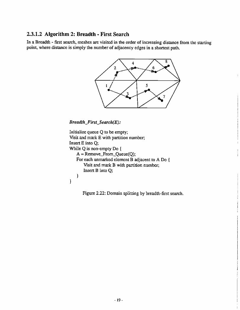
2.3.1.2 Algorithm 2: Breadth - First Search

In a Breadth - first search, meshes are visited in the order of increasing distance from the startingpoint. where distance is simply the number of adjacency edges in a shortest path.

Breadth_FirsCSearch(E):

Initialize queue Q to be empty;Visit and mark E with paroticn number;Insert E into Q;While Q is non-empty Do (

A = Remove_From_Queue(Q);For each unmarked element B adjacent to A Do {

Visit and mark B with partition number;Insert B into Q;

}

Figure 2.22: Domain splitting by breadth-first search.

- 19-

2.3.2 Group II: Domain -Axis scheme

Three algorithms to decompose the initial grid are based on the domain splitting along thedifferent defined axis. That is, define the domain axis by the basis geometry Cartesian Axis orPolar Axis. or pre-compute the Main Symmetry Axis according to the mesh elements in thedomain region. Then split the mesh elements along the axis into subdamain.

2.3.2.1 Algorithm 3: Cartesian Axis Splitting

Splitting the domain along the cartesian axis by sorting the X, Y, Z coordinates of centre of massof mesh elements. Several minor schemes are presented for selecting the suitable subdomains ondifferent problems. They are:

a. Row· Column Cartesian Axis Splitting: Suppose we need to split the domain into nr rowsby fie columns subdomains, where nr '" fie = np no. of processors. This scheme first splitsthe domain into nr subdomains by soning their Y coordinates. Then for each subdomain,the scheme splits it into nc subdomains again by sorting their X coordinates.

.........L·;··············,··············r··········

·········T.:··········,····~··········f···~············

riiT

-------- : ill splitting

: nc splitting

Sort their Y coordinates;Split the domain into nr subdomains along the Yaxis;For each splitted subdomain Do [

Sort their X coordinates;Split the domain into nc subdomains along the X axis;

Figure 2.23: Domain splitting by row-column canesian axis splitting.

·20·

b. Column - Row Cartesian Axis Splitting: The scheme is similar to a but it splits thedomain into nc subdomains by sorting their X coordinates first. Then for each subdomain,the scheme splits it into nr subdomains again by sorting their Y coordinates.

···•,· ..................: : : : nc splitting: ········i ~ .· .· .· .r····································· .· .· .: : -- : nr splitting.........................! : ""

· .· ....... . :'---. . .1-. : •!........................... ;:----

···

Column_Row_Cartesian():

Sort their X coordinates;Split the domain into nc subdomains along the X axis;For each splitted subdomain Do {

Sort their Y coordinates;Split the domain into nr subdomains along the Y axis;

Figure 2.24: Domain splitting by column-row cartesian axis splitting.

- 21 -

c. RCRC Cartesian Axis Splitting: This scheme is similar to a but it splits each domain into2 subdomains each time. That is, it splits the domain into 2 subdomains by sorting their Ycoordinates. Then for each subdomain, the scheme splits it into 2 subdomains again bysorting their X coordinates. Repeat these 2 steps until number of subdomains is reached.

i fi i

-~r---iJJI

RCRC_CartesianO:

------ .. : nr splitting

: nc splitting

While nr or nc is larger than 1 Do (If(nr> 1) {

For each splitted subdomains Do (Son their Y coordinates;Split the domain into 2 subdomains along the Y axis;

)nr /= 2;

)If(ne> 1) {

For each splitted subdomain Do {Son their X coordinates;Split the domain into 2 subdomains along the X axis;

)ne /= 2;

))

Figure 2.25: Domain splitting by RCRC cartesian axis splitting.

·22·

d. CRCR Cartesian Axis Splitting: This scheme is similar to c but it first splits domain into 2subdomains by sorting their X coordinates. Then for each subdomain, the scheme splits itinto 2 subdomains again by soning their Y coordinates. Repeat these 2 steps until numberof subdomains is reached.

. ...................: :. .'~---';---,-- : !- .· :· .: .

;, : .· ...................~ :----: :

.. ..

.. ..

.. .., ,

CRCR_Cartesian():

: nc splitting

............... : nr splitting

While nr or nc is larger than 1 Do {If(ne> 1) [

For each splitted subdomain Do {Son their X coordinates;Split the domain into 2 subdomains along the X axis;

}ne 1= 2;

}If(nr> 1) {

For each splitted subdomains Do {Son their Y coordinates;Split the domain into 2 subdomains along the Y axis;

}nr 1= 2;

)

Figure 2.26: Domain splitting by CRCR canesian axis splitting.

·23 .

e. Optimal Cartesian Axis Splitting: This scheme is similar to c and d. Each time it splits thedomain into 2 subdomains by selecting either the X axis or the Y axis which causes lesscommunication between these new generated subdomains. Repeat this step until numberof subdomains is reached.

Jednd i'-------, 2 .

td__ 3 __ # : split level number

.----,---'--1 s,,-',-_-'--,-__---,

td

OptimaCCariesian():

While np larger than I Do {For each splittect subdomain Do {

Son their X coordinates;Split the domain into 2 subdomains along the X axis;Compute the communication bisection width BWx;Son their Y coordinates;Split the domain into 2 subdomains along the Y axis;Compute the communication bisection width BWy;Select the one which has smaller bisection width;

)np/= 2;

)

Figure 2.27: Domain splitting by optimal cartesian axis splitting.

- 24 -

2.3.2.2 Algorithm 4: Polar Axis Splitting

Similar to the cartesian axis splitting, it splits the domain along the polar axis by sorting the R, 0,Z coordinates of cenrre of mass of mesh elements. In addition to the minor adjustment in cartesianaxis splitting, the various definitions of the original point are possible. Its calling process is asfollowing:

Define the original point as either:1. Centre of Inertia of meshes.2. Centre of Mass of meshes.3. User specified.

Map coordinates from Cartesian to Polar:(X, Y, Z) --> (R, e, Z)

Call relative Cartesian Axis Splitting routine:X --> R, Y --> e, Z --> Z

Map coordinates from Polar to Cartesian:(R, e, Z) --> ex, Y, Z)

Figure 2.28: Strategy for polar axis splitting.

a. Row • Column Polar Axis Splitting: This scheme first splits the domain into nrsubdomains by sarong their e coordinates. Then for each subdomain, the scheme splits itinto fie subdomains again by sorting their R coordinates.

................ : nr splitting

: nc splitting

Figure 2.29: Domain splitting by row-column polar axis splitting.

.. 25-

d. CRCR Polar Axis Splitting: This scheme is similar to c but it first splits domain into 2subdomains by sorting their R coordinates. Then for each subdomain, the scheme splits itinto 2 subdomains again by sorting their e coordinates. Repeat these 2 steps until numberof subdomains is reached.

: nc splitting

._- : nr splitting

\\

\!

/~,----_'~""_- ..",..., ,

/Y"'-;:::;:­

\/ / \

f l: 'i

f :i ' J

.~~ ./ /~fI/ :

,/ /./'......"...... ~ ~ ..- ....."" ........." .." .....-...._-_ ....-.~._.,.,.-,.-

//

/

Ii

Figure 2.32: Domain splitting by CRCR polar axis splitting.

e. Optimal Polar Axis Splitting: This scheme is similar to c and d. Each time it splits thedomain into 2 subdomains by selecting either the R axis or the e axis which causes lesscommunication between these new generated subdomains. Repeat this step until numberof subdomains is reached.

'ro3,2nd.....~ ....._ .•.,

~.,_... -"""--

# : split level number

Figure 2.33: Domain splitting by optimal polar axis splitting.

- 27 •

b. Column· Row Polar Axis Splitting: The scheme is similar to a but it splits the domaininto nc subdomains by sorting their R coordinates first. Then for each subdomain, thescheme splits it into nr subdomains again by sorting their e coordinates.

-_._.__..-._~r"'-' ,.'''..., ......

/I,i

\,

,/!

....-,_._._.,."./~ '-"'-...

--"_._"/

t

,,\\

\~iii!/,

: nc splitting

................ : nr splitting

Figure 2.30: Domain splitting by column-row polar axis splitting.

c. ReRC Polar Axis Splitting: This scheme is similar to a but it splits each domain into 2subdomains each time. That is, it splits the domain into 2 subdomains by sorting their ecoordinates. Then for each subdomain, the scheme splits it into 2 subdomains again bysorting their R coordinates. Repeat these 2 steps until number of subdomains is reached.

-- : nr splitting

: nc splitting

Figure 2.31: Domain splitting by RCRC polar axis splitting.

- 26-

2.3.2.3 Algorithm 5: Inertia Axis SplittingIn this scheme, it first pre-computes the main symmetry axis according to the centre of mass ofmesh elements. Then splits domain into several subdomains along the axis. Repeat this step untilthe number of subdomains is reached.

# : split level number

InertiaJlxis(J:

While np is larger than 1 Do (For each splitted subdomain Do {

Compute the main symmetry axis (1;Split the domain into os subdomains along axis a.;

)np 1= os;

Figure 2.34: Domain splitting by inertia axis splitting.

Computation ofthe main symmetry axis:Let A be the (2 x N) matrix of the mesh coordinates which belong to the current domainwith the original point as either:

1. Centre of Inertia of current meshes.2. Centre of Mass of current meshes.3. User specified.

The main ¥:mmetry axis is given by the Eigen vector corresponding to the largest Eigenvalue of A A.

- 28-

ill

2.3.3 Performance in domain decomposition algorithmIn the following table, we list the Maximum communication bisection bandwidth between processors. Where total means the maximumtotal edges one specified processor node joining with others, and I-by-l means the maximum edges between any two processor nodes.The first three examples are based on the engine rod head with different mesh density and processor number, while the fourth one isbased on the torque ann.

Max. communication bandwidth (total/1-by-l)Equal-sized with maximum difference of one remark

117m,4p 2191m,4p 2191m, 16p 3734m,16p

Neighborhood - Search Depth - First Search 26/13 176/111 97/49 160/70

Breadth ~ First Search 21/13 121/75 151/76 200/110

Domain - Axis Split Canesian Row - Column 9/5 36/20 42/18 63/26

Column - Row 8/4 34/18 48/20 73/31

R-C-R-C 9/5 36/20 43/18 63/27

CoR-CoR 8/4 34/18 47/20 87/29 Loriot 1988

Optimal 8/4 36/20 43/18 52/20

Polar Row- Column 18/10 64/36 61/30 68/23

Column - Row 16/10 65/43 57/27 152/74

R-C-R-C 18/10 64/36 61/28 81/38

CoR-CoR 16/10 65/43 57/27 80/53 Loriot1988

Optimal 8/5 35/21 35/18 64/21

Inertia Axis Split 20/12 99/56 79/34 161/96 Loriot1988

Table 1: Performance of domain decomposition algorithm

2.4 Subdomain boundary linking

After mesh decomposition, we need a linking routine to connect the new boundary for eachsubdomain before progressing mesh generation in parallel. Since the domain splitting will createmore than one subregion for one processor in some problems, the mesh generation scheme shouldbe capable of handling such case. New holes may be created also. Therefore. the linking routineneeds to separate the outer boundary polygon and the hole polygon. And identify a hole polygonbelongs to which outer boundary polygon. The linking algorithm is as follows:

Step!: Find the polygon list including outer boundary polygon and hole polygon:

While there is an unmarked mesh S which is on the boundary Do {Mark S and insert it into boundary list L~E1= S;Do (

Search an unmarked mesh Ez which is on the boundary and adjacent to E1;Mark Ez and insert it into boundary list L;El~q;

) While (E1 != 5);)

It needs the element-element adjacency list to search the boundary meshes, and node­element adjacency list to locate the next boundary mesh.

Step2: Separate the oUler boundary polygon and the hole polygon by the polygon locatingrecognition algorithm we described in sec. 2.3.2.

For each polygon PI Do (For each polygon Pzexcept Pi Do {

If (Locale]oIY(PI> P2l == "[nside") (Link PI to the hole list of P2;Break:;

)

- 30-

2.5 Final mesh generatingReviewed those previous literatures about the parallel mesh generation: In [Loho 92], it eithergenerates mesh of each subdomain separately in parallel, then generates mesh of the inter­subdomain region sequentially. Or generates mesh of the inter-subdomain region sequentially,then generates mesh of each subdomain separately in parallel. In both cases, they need tocommunicate between processor nodes for generating mesh in the inter-subdomain region. orgenerating them sequentially. Furthermore, when generating mesh in each subdomain. it does nothave a global smooth node distribution.

In our approach. since we introduce the quadtree dala structure to supervise the node distribution,it is easy and efficient to refine it globally before generating mesh in parallel. Therefore, duringthe progress of parallel mesh generation, it does not need the communication between processornodes. And because of the global smoothness of the node distribution, it will generate better meshelements.

In addition, we can use the same algorithm and same code in sequential mesh generator togenerate the unstructured mesh on each subdomain in parallel. And the same code for parallellocal mesh smoothing and side swapping, sequential global mesh smoothing and side swapping.These will reduce the development effort and cost.

I. Ponn the initial grid.2. Decompose domain.3. Link subdomain boundary.

//4-2. Parallel mesh generation.4-3. Local mesh smoothing.4-4. Local side swapping.

14-1. Refine quadtree node distribution. ~1/

Node

K ...

/ 4-2. Parallel mesh generation.

4-5. Global mesh smoothing. ~_._. 4-3. Local mesh smoothing.

4-6. Global side swapping...~._._..~._._ ..~ 4-4. Local side swapping.

Node

15. Optimal mesh partition. I

Host

Figure 2.35: Strategy of final mesh generating in paral1el.

·31 .

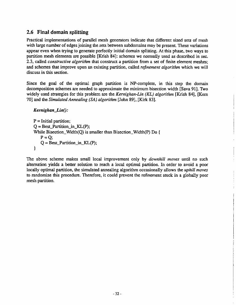
2.6 Final domain splitting

Practical implementations of parallel mesh generators indicate that different sized sets of meshwith large number of edges joining the sets between subdomains may be present. These variationsappear even when trying to generate perfectly initial domain splitting. At this phase. two ways topanition mesh elements are possible [Krish 84]: schemes we normally used as described in sec.2.3, called constructive algorithm that construct a partition from a set of finite element meshes;and schemes that improve upon an existing partition, called refinement algorithm which we willdiscuss in this section.

Since the goal of the optimal graph partition is NP-complete. in this step the domaindecomposition schemes are needed to approximate the minimum bisection width [Sava 91]. Twowidely used strategies for this problem are the Kernighan-Lin (KL) algorithm [Krish 84], [Kern70J and the Simulated Annealillg (SA) algorithm [John 89], [Kirk 83].

Kernighan_Lin():

P = Initial partition;Q = Bes,-Partition_in_KL(P);While Bisection_Width(Q) is smaller than Bisection_Width(P) Do (

P=Q;Q = Best_Partition_in_KL(P);

)

The above scheme makes small local improvement only by downhill moves until no suchalternation yields a better solution to reach a local optimal partition. In order to avoid a poorlocally optimal partition, the simulated annealing algorithm occasionally allows the uphill movesto randomize this procedure. Therefore, it could prevent the refinement stuck in a globally poormesh partition.

- 32-

2.7 Fully automatic mesh adaptationAfter generating an initial mesh and performing a finite element analysis, our automatic finiteelement modeling program is able to measure the local error, determine the areas of the meshwhere the solution is not sufficiently accurate, and refine mesh in the specified area. That is. it canautomatically perform as many iterations of analysis, error estimation, and mesh improvement asrequired to reach the desired degree of accuracy.

Since only displacements are guaranteed to be continuous in displacement based finite elementanalysis. and stresses are not assured to be continuous. The stresses on those nodes sharing bydifferent elements will not match. Therefore. the feature of the posteriori error estimators we arecurrently used in P/FEA is based on the difference between the averag.~d and the unaveragedelement stresses. [Zienk 87]

Eo=cr'-cr

where cr is the unaveraged element stresses which are always directly computed by the Gausspoints and extrapolated to the node points to obtain the node stresses. And cr' is the averagedelement stresses which are obtained to produce a continuous stress field. In general, the errorestimator Eo will be nonzero unless the finite element analysis result is exact. Based on the energynonn to compute the element stress error for the ith element as,

IIEo l1 2 = f {EolT[K]-1 {EoldQj

Q;

where [K] is the material stiffness matrix. And the refinement strategy is dependent on thespecified accuracy requirement of a certain minimum percentage error in the energy nonn.

Figure 2.36 shows an example of the fully automatic mesh adaptation in one adaptive step byusing P/FEA. In our approach, mesh refinement is done by reduction of the mesh size (h­refinement) which is normal to most engineering problems.

- 33 -

15 refine pointsIn

one adaptive step..79 nodes, 117 elements

,

-', k; '~, .-,.- - j -I _~

~ "..':'-:': .t.ffi~ ',,--":~. , " '-- .. ,- '.

Defonned shape

136 nodes. 222 elements

Deformed shape

...!ill

SIresS: <-7789.59. 6769.68> Stress: <-16446.6. 8286.24>

:I·~I.•..,. ;;~..•~~"d.......-.-..-..­-,:..w

Error. O.164/2.l0E-5 Error: 1.427/8.68E-S

Figure 2.36: Fully automatic mesh adaptation in one adaptive step by using P/FEA.

- 34-

2.8 Performance in parallel mesh generationFor the two examples, engine rod head and torque ann, we have discussed the performanceevaluation including Speedup and Utilization which shows the three states - busy. overhead, andidle - as a function of time for each processor. We categorize each processor as idle if it hassuspended execution awaiting a message that has not yet arrived or it has ceased execution at theend of the run, overhead if it is executing the communication stuff in program, and busy if it isexecuting the portion of program other than the communication stuff. [Geist 92] [Geist 90] [Heath93]

2.8.1 Performance 1 - Engine rod head

.­'sp....dupl.d"t"· _

"o•••••

..4•••.

ill HI"Humber or prOC~5&Or5

Utilization Count

states of idle, overhead, andbusy as function of time.

Utilization Summary

overall cumulative percentageof time in idle, overhead, andbusy states.

'.

- --"" o

Figure 2.37: Performance of parallel mesh generation - Engine rod head.

• 35 •

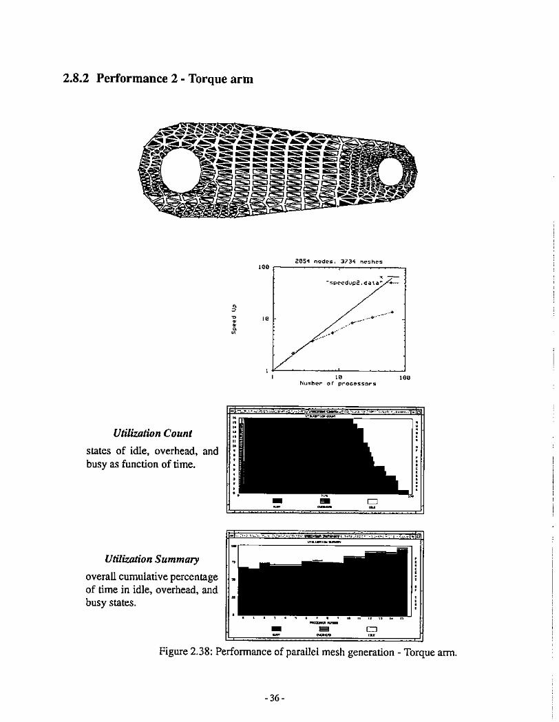
2.8.2 Performance 2 - Torque arm

,--s".."dup2.dal""

Utilization Count

states of idle. overhead, andbusy as function of time.

•o"••o•

"

-

•

.•.-'

l~ 100Nu~b"r or processors

D,~

- ,~

Utilization Summary

overall cumulative percentageof time in idle. overhead, andbusy states.

, .- . ...--

., ~ ....'. -. ", ,_ w

" "D

Figure 2.38: Perfonnance of parallel mesh generation - Torque arm.

- 36-

3 Parallel Shape OptimizationShape Optimization of a large complex system with a great deal of variables and constraints isusually time consuming task. It might be more efficient to divide the system into several smallersubsystems. In general. an optimization problem involving many variables and constraints cannotbe decomposed into independent subproblems which can be independently optimized.Nevertheless. the methods in this article do pennit the decomposition of shape optimization intosubproblem which solved independently in a parallel manner yields the whole system optimum.The analysis and shape optimization is implemented using the domain decompositionmethodology which is based on the static parallel mesh and mesh-splitting described in ParallelAdaptive Mesh Generation. The domain decomposition solvers of the parallel ELLPACK system[Holls 92] are currently used for the analysis. For the shape optimization problem we aredeveloping two level semi-optimal algorithms based on the local and global mesh anddecomposition data [Ding 86].

3.1 Formulation of parallel shape optimization processThe two level semi-optimal algorithm is a hierarchical strategy in which there are two levels ofoptimization schemes. The lower-level which solves the optimization subproblem on the localmesh of each subsystem independently in a parallel manner. And the higher-level, controls theglobal mesh, coordinates the action of the lower-level units so that the optimum of the originalproblem is obtained.

Consider the general optimization problem of choosing the variables {X} such that

Z = F({X}) => min.

(h«X})) = [0)(g«X})} $ {OJ

[XL} $ {X} $ [XU}

where F({X}) is the objective function. (h«X})} and (g({X})} are set of equality and inequalityconstraints. And (XL) and {XU} are the lower and upper bound vector of [X}.

Decomposition of the optimization problem is carried out by first converting the problem into atwo level form with separate and distinct tasks assigned to each level. That is, we split apart of thevariables and constraints for each subdomain which do not interact with others in othersubdomain to form the 10wer~level units. Then choose the dependent variables, calledcoordinating variables, to the higher-level unit which correspond to an overall system optimum.In general, the lower-level and the higher-level problems are solved iteratively.

There are two different ways to convert a given problem into two-level schemes which are themodel coordination method and the goal coordination method [Kirsch 75].

·37·

3.2 Model coordination method

We partition the vector {Xl into two subvectors, {S} and {Tl

(X)T ~([S}T. (T)T)

in which {S) is called the suhvector of coordinating variables between the subdomains and {TI isthe subdomain variables which we decompose it into subdornains as follows:

(TIl

(T) = {T;}

[Tn)

where (Td represents the subdomain variables associated with the ith subdomain and n is thenumber of subdomains. Decomposition is effected so that the objective function and the equalityand inequality constraints can be rewritten in the following fonn:

n

Z = F({X}) = I Fi({S). {T,))i = I

(ht([S). (TIl))

(h) = [hillS). (T;}))

[hn«(S}. (Tn))}

(gl«(S). [TIl))

(g) = [g;«(S). (Ti)))

(gn([S). (Tn)))

That is, the coordinating variables {S} may appear in all expressions. while the subdomainvariables {T;} appear only in the term Fi of the ohjectivefunction and the equality selS (hi) = (0)and the inequality set [gi) ~ (0). Based on this. the original problem can be reslated as:

n

Z = I F i ((S). (T,}) => millj = 1

(hi([S). [Ti))) = (OJ(gi((S). (Ti))) ~ (0)

[SL) ~ (S) ~ (SU)

{Th ~ (Ti) ~ (TiU)

i = 1, "', ni = 1, "', n

i = 1, ... , n

again. (SL). (SU). (Th. and [TiU) are the lower and upper bound vectors for the decomposedsubproblems.

- 38-

The two level problem can be solved iteratively as following steps:1. Choose an initial value for the coordinating variables {SO}.2. For a given {SO} solve the n independent lower-level subproblems in a parallel manner.3. Modify the value of {SO} so that higher-level is optimum.4. Repeat steps (2) and (3) until the global optimum is achieved.

The fonnulation of these two levels is as follows:

Lower-level problem:For a given fixed value of coordinating variables {SO}. the problem in this level can bedecomposed into n independent subproblems. Each of them stated as: find {Til such that,

Zi = Fi({S°j, (Til) ~ min.

{hi({S°j, (Ti))} = {OJ{gi({S°j, {Ti))}"; {OJ

(Th ,,; {Ti} ,,; {TiU}

Higher-level problem:The task in this level is to find a (SO) such that,

n

Z = I F i ({ s"J, {T,} ) => mini = 1

while all ITi } are fixed.

Host

Find {S } such that:

"z= L.Fi({S°},{Tj})~mjn;: I

{SO,

Find {Til such that:

Zl = FI({S°J, lTd>~ min.(h,(IS°), {T, Il} = {O}Ig,({S°}, {T, Il} < 10J

{TIL}:$; {Ttl:s: IT.UI

lTdISO}

Find {Tn} such that:

Zn =Fn(ISol.ITnJ) ~ min.Ih,({SO}. IT,ll} = (01{g,({SO}.{T,Il} < {O}

fTnLJ:$;ITnl:$;{TnUI

~M ~M

Figure 3.1: Model coordination method for parallel shape optimization.

- 39 -

3.3 Goal coordination methodIn this scheme, the overall system is decoupled. That is, all links between its subsystems aredisconnected. And the variables {S} called the illterconnectioll variables are now permitted todiffer on either side of each subsystem interface. Assign {Si} as the vector of the above variablesassociated with the ith subsystem, then the vector of variables in the ith subsystem becomes

[X;}T = ( [Si)T, (T;}T)

That is, while {Td and [Ti+d represent different variables, {Sil and {Si+d may represent thesame variables with different values. [Sil and {Td are chosen so that the variables {XiJ appearonly in the tenn Fj of the objective function and the equality sets {hi} = {O} and the inequality set{gil $ (OJ.

Z = F({X}) = IF;({X;})i = 1

[hi({Si}, (Ti ))) = {OJ[gi({Si}, (T;}») $ {OJ

(SL) $ [S;} $ [SUi

{Th $ {Til $ (TiU)

i = I, "', ni=I, ... ,n

i = 1, ...• n

i = I, .... n

Therefore, the optimum of the overall system is achieved when the interaction-balance conditionsto he satisfied:

i= 1, ...,n-l

Subsystem i: Subsystem i+ I:

Variables:{Sd =ISi.i_tI{Si,i+tl

{Til

Yariables:(Si+1 J =ISi+l, i}{Si+l,i+21

Figure 3.2: The interaction-balance conditions for the overall system.

To obtain the optimum of the overall system, we need to define a new vector of coordinatingvariables,

And introduce an extra term of penalty function, vanishing at the optimum when the interaction­balance condition is satisfied, in the new objective function which is defined by.

n n - 1

Z = F({X}, {A}) = IF;({X;}) + I {Ai.i+j)T({Si.'+!} - {S;+!.,»;=1 ;=1

- 40-

n

Expanding the tenn of penalty function into the following fonn:n-I

I {A';,;+I}T({S;,;+I} - {S;+I,;l) = I (A)T{S;li=l i::l

And the objective function of the dual optimization problem becomes.

n

2 = F( {X}, (A}) = I (F;( (X;}) + (A)T (Si})i:: I

In general, for a given initial value of (A.oJ, it can be shown that,

(2 (A) =F ({X), {A})) ;" (D (AD) =;tl (F i ({X;}) + g?} T {S;l) )

That is, D(A~ is a lower bound of the objective function. If F( [X}, [AI) has a saddle point, wewill obtain

max. D(A) = min. F({X}, (AI)

Therefore. the two level problem can be solved iteratively as following steps:1. Choose an initial value for the coordinating variables {AoJ.2. For a given {Ao} solve the n independent lower-level subproblems in a parallel manner.3. Modify the value of {AO} in the higher level so that the objective function increase.4. Repeat steps (2) and (3) until the maximum objective function is achieved.

The formulation of these two levels is as follows:

Lower-level problem:For a given fixed value of coordinating variables rA.o}, the problem in this level can bedecomposed into n independent subproblems. Each of them stated as:

find [XiIT = ([Si}T, [T;)T) such that,

Zi = Fi([Xil) + p"i0}T [S;) =) min.

{hi«Xi))) = {Ol{gi«Xi))) ,,; (0)

{Xh ,,; [X;) ,,; (XiU)

- 41 -

Higher-level problem:The task in this level is to find a {".o} so that the interaction-balance condition is satisfied.That is, to make {Si. i+I} and {Si+1, i} be equal. this is achieved by,

n

Z = F({Xj, (A.}) = I (F,({X,}) + (A.,)T{S,)l =>maxi:::: 1

while all {T;) are fixed.

Host

Find IA: I such that:

"Z = L (F,({X,}) + lA,lT{S,}) ~m~

;=1

IX,}

Find {Xd such that:

Z, =F,({X,}l + IA,'IT IS,} => min.

Ih,IIX,})J =101Ig,({X,)J I ~ 10J{X,L}:s; IXiI::S; {XlUI

Node

i=l. .... n-l

IX,J

Find (XnI such that:

'Zn = Fn({XnJ) + IAn°IT ISnl ~ min.Ih,({X,1l1 = 10JIg,({X,lll ~ {OJ{XnLI:S; (Xn}:S; IXnUj

Node

Figure 3.3: Goal coordination method for parallel shape optimization.

-42 -

3.4 Examples of parallel shape optimizationFigure 3.4 and 3.5 show two examples of the parallel shape optimization with the concept of themodel coordination method and the goal coordination method.

3.4.1 Example 1 - Parallel shape optimization with load case #1

136 nodes, 222 elements

Shape Optimization

Z = An:a = min.

oS 16000-0'::>21000

O.5SSi Sl.O i=I, ...,50.1 STj•j S 1.0 i = I. 3

j = I, 205 ST;.j S l.Oi =2. 4

j = I, 2

.. 127 nodes, 189 elements

-.,..- -

Deformed shape

-.~ -."

-I~.-.

~I';l-..--.-::J:jSlress: <-20258.8. 15530.5>

L

L

"'"- "

~.--"-"-"-"~.....ill

-_.•_.-.:: :~;

Defonned shape

Stress: <-16446.6, 8286.24>

Figure 3.4: parallel shape optimization with load case #1.

- 43 -

3.4.2 Example 2 • Parallel shape optimization with load case #2

s,Shape Optimization

TI .] T}.]

156 nodes, 264 elements 156 nodes, 244 elements

0' 518000-0" s; 22000

0.55S;51.0 i=I •... ,3O.IST,.jS 1.0i = 1.3

j = 1, 20.5 s: Ti.j.s; 1.0 i = 2, <I

j = 1,2

0.5 STi.):S 1.0i = 1.3

Z=A~a~min.

s,s,

Deformed shape

---.-

-Deformed shape

Stress: <-21490.4.17731.9>

-I_.-.::;:;_.-~I-~.--"-"-,'"- ..l:.llJ

Stress: <-17643.3. 13895.8>

Figure 3.5: parallel shape optimization with load case #2.

·44-

4 References

[Hous 92] E. N. Houstis and J. R. Rice, "Parallel ELLPACK: A development and problemsolving environment for high performance computing machines", ProgrammingEnvironments for High-Level Scientific Problem Solving (P.W. Gaffney and E.N.Houstis, Eds), North-Holland, (1992) 229-241.

[Chri 91] N. P. Chrisochoides, E. N. Houstis and C. E. Houstis, "Geometry based mappingstrategies for PDE computations", Proceedings of the International Conference onSupercomputing, Cologne-Germany, (June 1991) 128-135.

[Wu 93] Poting Wu and E. N. Houstis, "XXoX: An interactive X-window based user interfacefor the XoX solid modeling library", CAPO Technical Report, Purdue University,Department ofComputer Sciences, TR-93-08, (January 1993) 1-47.

[XoXE 92] SHAPES Geometric Computing System - Geometry Library Reference Manual (CEdition), XOX Corporation, (1992).

[XoXR 92] SHAPES Geometric Computing System - Graphics Library Reference Manual (CEdition), XOX Corporation, (1992).

[Patran 92] PATRAN, A Division of PDA Engineering - PATRAN Plus User Manual, Vol. 1 & 2,PDA Engineering, PATRAN Division.

[Lohn 92] Rainald Lohner, Jose Camberos and Marshal Merriam, "Parallel unstructured gridgeneration", Computer Methods in Applied Mechanics and Engineering 95, (1992)343-357.

[Khan 91] A. J. Khan and B. H. V. Topping, "Parallel adaptive mesh generation", ComputingSystems in Engineering 2·1, (1991) 75-101.

[Cheng 89] Fuhua Cheng, Jerzy W. Jaromczyk, Junnin-Ren Lin, Shyue-Shian Chang and Jei­Yeou Lu, "A parallel mesh generation algorithm based on the vertex label assignmentscheme", International Journal for Numerical Methods in Engineering 28, (1989)1429-1448.

[Lo 91] S. H. La, "Automatic mesh generation and adaptation by using contours",International Journalfor Numerical Methods in Engineering.

[Bykat 76] A. Bykal, "Automatic generation of rriangular grid: I-Subdivision of a generalpolygon into convex subregions. II-Triangulation of convex polygons", InternationalJournalfor Numerical Methods in Engineering 10, (1976) 1329-1342.

- 45 -

[Sadek 80] Edward A. Sadek, "A scheme for the automatic generation of triangolar finiteelements", International Journal for Numerical Methods in Engineering 15. (1980)1813-1822.

[De1j 90] K. Deljouie-Rakhshandeh, "An approach to the generation of triango1ar gridspossessing few obtuse triangles". International Journal for Numerical Methods inEngineering 29, (1990) 1299-1321.

[Samet 84] Hanan Samet, "The quadtree and related hierarchical data structures", ComputingSurveys 16 - 2, (1984) 187-260.

[Samet 82] Hanan Samet. "Neighbor finding techniques for images represented by quadtrees",Computer Grophics and Image Processing 18, (1982) 37-57.

[Samet 85] Hanan Samet and Clifford A. Shaffer, "A model for the analysis of neighbor findingin pointer-based quadrrees", IEEE Transactions on Pattern Analysis and MachineIntelligence PAMI-7 - 6, (1985) 717-720.

[Samet 89] Hanan Samet, "Neighbor finding in images represented by octrees", Computer Vision,Graphics, and Image Processing 46, (1989) 367-386.

[Zienk 87] O. C. Zienkiewicz and J. Z. Zhu, "A simple error estimator and adaptive procedurefor practical engineering analysis", International Journal for Numerical Methods inEngineering 24, (1987) 337-357.

[Lori 88] M. Loriot and L. FezQui, Mesh-splitting preprocessor. unpublished manuscripts,(1988).

[Sava 91] John E. Savage and Markus G. W1oka, "Parallelism in graph-partitioning", lournai ofParallel and Distributed Computing 13, (1991) 257-272.

[Kern 70] B. W. Kernighan and S. Lin, "An efficient heuristic procedure for partitioninggraphs", The Bell System Technical lournai 49, (February 1970) 291-307.

[Krish 84] Balakrishnan Krishnamurthy, "An improved min-cut algorithm for partitioning VLSInetworks". IEEE Transactions on Computers C-33-5, (May 1984) 438-446.

[John 89] David S. Johnson, Cecilia R. Aragon, Lyle A. McGeoch, and Catherine Schevon,"Optimization by simulated annealing: An experimental evaluation; Pan I, Graphpartitioning", Opera/ions Research 37-6, (November-December 1989) 865-892.

[Kirk 83] S. Kirkpatrick, C. D. Gelat!, Jr., and M. P. Vecchi, "Optimization by simulatedannealing", Science 220-4598, (13 May 1983) 671-680.

·46 -

[Farhat 93] Charbel Farhat and Michel Lesoinne, "Automatic partitioning of unstructured meshesfor the parallel solution of problems in computational mechanics", InternationalJournal!or Numerical Methods in Engineering 36, (1993) 745-764.

[Ding 86] Yunliang Ding, "Shape optimization of structures: A literarure survey", Computers &Structures 24 • 6, (1986) 985-1004.

[Haftka 86] Raphael T. Haftka and Ramana V. Grandhi, "Structural shape optimization - Asurvey", Computer Methods in Applied Mechanics and Engineering 57, (1986) 91­106.

[Hint 91-1] E. Hinton, N. V. R. Rao, and M. Ozakca, "An integrated approach to structural shapeoptimization of linearly elastic structures. Part I: General methodology", ComputingSystems in Engineering 2-1, (1991) 27-39.

[Hint 91-2J E. Hinton, M. Ozakca, and N. V. R. Rao, "An integrated approach to structural shapeoptimization of linearly elastic structures. Part II: Shape definition and adaptivity",Computing Systems in Engineering 2·1, (1991) 41-56.

[Brai 84] V. Braibant and C. Fleury, "Shape optimal design using B-splines", ComputerMethods in Applied Mechanics and Engineering 44, (1984) 247-267.

[Kirsch 75] Uri Kirsch, "Multilevel approach to optimum structural design", Journal of theStructural Division, ASCE 101· ST4, April 1975, 957-974.

[Char 91] Mladen K. Chargin, lngo Raasch, Rudolf Bruns, and Dawson Deuenneyer, "Generalshape optimization capability", Finite Elements in Analysis and Design 7, (1991)343-354.

[EI91] M. E. M. El-Sayed and C. K. Hsiung, "Design optimization with parallel sensitivityanalysis on the CRAY X_MP", Structural Optimization 3, (1991) 247-251.

[SOOo 88] Efthimios S. Sikiotis and Victor E. Saouma, "Parallel structural optimization on anetwork of computer workstations", Compurers & Structures 29-1, (1988) 141-150.

[Vander 89]G. N. Vanderplaats, "Effective use of numerical optimization in structural design",Finite Elemenrs in Analysis and Design 6, (1989) 97-112.

[Botkin 86] M. E. Botkin, R. 1. Yang, and 1. A. Bennett, "Shape optimization of three-dimensionalstamped and solid automotive components", The Optimum Shape: AutomatedStructural Design, Plenum Press, New York, (1986) 235-262.

[Bennet 85]1. A. Bennett and M. E. Botkin, "Structural shape optimization with geometricdescription and adaptive mesh refinement", AlAA Journal 23-3, (1985) 458-464.

- 47 -

[Vander 86] Garret N. Vanderplaats and Hiroyuki Sugimoto, "A general-purpose optimizationprogram for engineering design", Computers & Structures 24·1, (1986) 13-21.

[Rogers 86]James L. Rogers and Jean-Francois M. Barthelemy, "An expen system for choosingthe best combination of options in a general purpose program for automated designsynthesis", Engineering with Computers 1, (1986) 217-227.

[Vander 85] Garret N. Vanderplaats, Hirokazu Miura, and Mladen Chargin, "Large scale structuralsynthesis", Finite Elements in Analysis and Design 1, (1985) 117-130.

[Geist 92] G. A. Geist, M. T. Heath, B. W. Peyton, and P. H. Worley, "A users' guide to PICL, aportable instrumented communication library", Technical Report ORNLfIM-1l616,Oak Ridge National Laboratory, Oak Ridge, TN, February 1992.

[Geist 90] G. A. Geist, M. T. Heath, B. W. Peylon, and P. H. Worley, "PICL: a portableinstrumented communication library, C reference manual", Technical Report ORNUTM-1l130, Oak Ridge National Laboratory, Oak Ridge, TN, July 1990.

[Heath 93] Michael T. Heath and Jennifer Etheridge Finger, "ParaGraph: A tool for visualizingperformance of parallel programs", Oak Ridge National Laboratory, Oak Ridge, TN,Apri11993.

- 4B-