parallel computing with load balancing on heterogeneous distributed systems

Parallel computing with load balancing on heterogeneous

distributed systems

Primoz Rus, Boris Stok*, Nikolaj Mole

Faculty of Mechanical Engineering, University of Ljubljana, Askerceva 6, Ljubljana SI-1000, Slovenia

Received 13 September 2002; revised 9 December 2002; accepted 9 December 2002

Abstract

In the present work, the parallelization of the solution of a system of linear equations, in the framework of finite element computational

analyses, is dealt with. As the substructuring method is used, the basic idea refers to a way of decomposing the considered spatial domain,

discretized by the finite elements, into a finite set of non-overlapping subdomains, each assigned to an individual processor and

computationally analysed in parallel. Considering the fact that Personal Computers and Work Stations are still the most frequently used

computers, a parallel computational platform can be built by connecting the available computers into a computer network. The

incorporated computers being usually of different computational power and memory size, the efficiency of parallel computations on such a

heterogeneous distributed system depends mainly on proper load balance. To cope the balance problem, an algorithm for the efficient load

balance for structured and free 2D quadrilateral finite element meshes based on the rearrangement of elements among respective sub-

domains, has been developed.

q 2003 Elsevier Science Ltd. All rights reserved.

Keywords: Parallel computing; Heterogeneous computer system; Load balancing

1. Introduction

With the development of both, the computers technology

on one hand and computational methods on the other hand,

technical problems, which can be computationally simu-

lated by corresponding numerical models, become more and

more comprehensive. In consequence, along with facilitated

investigations and increased physical understanding

achieved, the efficiency of problems solutions, especially

in R&D stage, is considerably improved. Unfortunately,

numerical treatment of complex physical problems by

discrete methods of analysis can lead to very large systems

of linear equations. Computer systems development in the

sense of parallel computers and connecting of single

computers into a group via a network, offer a possibility

for the solution of such large-size problems even when the

capability of a single computer is exceeded. Irrespective of

the parallelization strategies used, the issue of proper load

balancing, enabling highest computational efficiency,

becomes very important when the distributed computer

system is heterogeneous [1]. This is especially true for non-

linear and non-stationary problems, which are solved

incrementally, usually with much iteration needed within

an incremental step.

Domain decomposition has become a widely adopted

technique to develop parallel applications based on discrete

approximation methods [2], and in particular by the finite

element method [3–6] and the boundary element method

[7]. The FE computational scheme used in our parallel

approach relies on the substructuring method, according to

which the general problem equation, resulting from the

consideration of the whole problem domain, can be split into

a series of equations, pertaining to the individual sub-

domains, as obtained by the corresponding domain

decomposition. These equations can be solved only after

the solution of the associated interface problem, which

involves the complete determination of the physical

variables on the interfaces between adjacent subdomains.

For the solution of the interface problem direct [4] or

iterative solvers [2,6,8] may be applied. Here, use of the

direct solution approach will be made.

The efficiency of using the domain decomposition on the

heterogeneous system depends on a way the computational

0965-9978/03/$ - see front matter q 2003 Elsevier Science Ltd. All rights reserved.

doi:10.1016/S0965-9978(02)00141-2

Advances in Engineering Software 34 (2003) 185–201

www.elsevier.com/locate/advengsoft

* Corresponding author.

E-mail addresses: [email protected] (P. Rus), [email protected]

lj.si (B. Stok), [email protected] (N. Mole).

http://www.elsevier.com/locate/advengsoft

domain is divided into subdomains, and how the latter are

assigned to the processors. Clearly, the subdomains should

be assigned in such a way that all processors would be

engaged in the computation evenly, thus the execution of

the allocated task taking approximately the same time. Due

to heterogeneity of the considered computing system it is

obvious, that allocation of the same amount of work to each

processor would result in inefficient parallel computation,

with several processors being possibly idle even for a long

time. Though considering the established standard computer

performance characteristics, it is almost impossible to define

a priori such a balance ratio between the computers in the

heterogeneous distributed system that would yield efficient

parallel computation. This is mostly due to the fact that

actual computational performance of a processor, perform-

ing the allocated work, depends exclusively on the number

of degrees of freedom and the number of interface variables,

pertaining to the assigned subdomain.

Load balancing for heterogeneous parallel systems is a

relatively new subject of investigation with a less-explored

landscape. Due to reasons discussed above, static load

balancing based solely on the prior knowledge of com-

ponents performance, is rarely a successful option. In

consequence, some sort of dynamic load balancing must be

applied. One way of doing it is by decomposing the problem

into small and independent tasks, sending a task to each

component of the computing system, and sending a new task

to a component when it completes the previous task [9,10].

In this approach, the issue of load imbalance is actually

ignored. Another possibility, which seems to be reasonable

only when the range of processing power is broad, is given

by asymmetric load balancing [11]. A real dynamic load

balancing technique should use observed computational and

communication performance to predict the time a task

would complete on a given component and the time needed

to query the component. This approach, which can be

addressed in many different ways as standard clock

approach [12], a dynamic distributed load balancing based

on aspect ratio [13,14], a diffusion algorithm for hetero-

geneous computers [15], is also the path we are following.

In order to achieve efficient computation a strategy is

developed, which in course of ongoing of incremental

computation automatically rearranges the subdomains in

sense of the load balancing. Considering a solution of the

problem, equations presents the predominant source of CPU

time consumption the load balancing is conceived upon

computing times, realized on a processor while establishing

all the respective subdomain data needed for the setting and

solution of the interface problem. As the freely accessible

METIS program [16], which was used for mesh partitioning,

proved some deficiencies associated with the automatic load

balancing. We have developed an algorithm for the

rearrangement of elements among subdomains. The com-

putations being most efficient with smaller number of

interface nodes, the algorithm is developed by considering

minimization of the interface nodes.

All communications and data transfers among com-

puters in the distributed system were managed through

the ‘Parallel Virtual Machine (PVM)’ communication

library [17].

2. Substructuring method

Let us consider a physical problem defined on a domain

V. In the context of the FEM, the continuous problem is

discretized to yield a finite set of nodal primary and

secondary variables, u and f, respectively. The relationship

between them is given by the matrix equation Ku ¼ f: The

problem is fully determined by specifying the correspond-

ing boundary conditions u ¼ ur on Gu and f ¼ fm on Gf :

The basic idea of the substructuring method [3–5] is in

decomposing the considered spatial domain V into a finite

set of non-overlapping subdomains Vs (Fig. 1). As a result

of the domain decomposition any two adjacent subdomains

share the common interface boundary GI ; with conditions of

physical continuity and consistency to be respected on it.

Following the performed decomposition of the domain

V into Ns subdomains Vs; the general problem equation

Ku ¼ f must be accordingly restructured, with equations

associated to internal nodes of each subdomain numbered

first, and equations associated to interface nodes numbered

last. In general, the resulting system of equations has the

following matrix form:

K11 0 · · · 0 K1I

0 K22 · · · 0 K2I

..

. ... . .

. ... ..

.

0 0 · · · KNsNsKNsI

KI1 KI2 · · · KINsKII

266666666664

377777777775

u1

u2

..

.

uNs

uI

8>>>>>>>><>>>>>>>>:

9>>>>>>>>=>>>>>>>>;¼

f1

f2

..

.

fNs

fI

8>>>>>>>><>>>>>>>>:

9>>>>>>>>=>>>>>>>>;

ð1Þ

Fig. 1. Decomposition of the considered domain into two subdomains.

P. Rus et al. / Advances in Engineering Software 34 (2003) 185–201186

The system matrix K, usually also called the stiffness

matrix, has a block-arrowhead form. Each diagonal

submatrix Kss represents the local stiffness of the subdomain

Vs; while the submatrix KII is the stiffness associated with

the nodal variables at the interface GI : An off-diagonal

submatrix KsI denotes the coupling stiffness between the

subdomain Vs and the interface GI : Accordingly, the vector

of primary variables u is partitioned into the subvectors us,

which correspond to the DOF pertaining to the interior of

the subdomains Vs; and the subvectors uI, associated with

DOF on GI : Similarly, fs denotes the part of the loading

vector f associated with the interior of Vs, while fI is a

subvector corresponding to the interface variables on GI.

If the matrix Eq. (1), is further restructured with respect

to given boundary conditions for the primary and secondary

variables, u ¼ ur on Gu and f ¼ fm on Gf ; respectively, the

following solution path can be traced

† Step 1. Given

KpIIu

pI ¼ fpI ð2Þ

solve for the unknown primary variables umI at interface

nodes. The respective matrix and vectors in Eq. (2) are

defined as

KpII ¼ Kmm

II 2XNs

s¼1

Kps

upI ¼ um

I ð3Þ

fpI ¼ fmI 2 Kmr

II urI 2

XNs

s¼1

fps

where

Kps ¼ ðKmm

sI ÞTðKmmss Þ21Kmm

sI

fps ¼ KmrIs ur

s 2 ðKmmsI ÞTðKmm

ss Þ21ðfms 2 Kmr

ss urs 2 Kmr

sI urI Þ

ð4Þ

† Step 2. With umi being determined in Step 1 solve for the

primary variables ums at internal nodes of each subdomain

Vs; ðs ¼ 1; 2;…;NsÞ

ums ¼ ðKmm

ss Þ21ðfms 2 Kmr

ss urs 2 Kmr

sI urI 2 Kmm

sI umI Þ ð5Þ

† Step 3. Finally, the unknown secondary variables at

internal nodes of each subdomainVs ðs ¼ 1; 2;…;NsÞ and

at interface nodes, frs and fr

I ; respectively, can be

determined

frs ¼ Krr

ssurs þ Krr

sI urI þ Krm

ss ums þ Krm

sI umI fr

I

¼ KrrII ur

I þ KrmII um

I þXNs

s¼1

½KrrIs ur

s þ KrmIs um

s � ð6Þ

The fact, that the local stiffness submatrices, associated with

the internal primary variables, Kmmss ;Kmm

sI ;Kmrss ;K

mrsI and Kmr

Is ;

are uncoupled is advantageous. It can be exploited for

concurrent computation of the matrices Kps and vectors fps for

each subdomain Vs; provided each subdomain computations

are allocated to a different processor.

The parallel implementation of the problem solution, as

determined by the algorithms 2–6 of the substructuring

method, is schematically presented in Fig. 2. From the

scheme, the sequence of computing steps with respective

objects of computations defined, as well as the master/slave

allocation of a particular computation can be seen.

3. Performance characterization of heterogeneous

computers

In order to take advantage of the mathematical structure of

the domain decomposed problem which enables concurrent

computing, it is of major importance for such a computation

to be efficient on heterogeneous distributed systems, that the

allocated processor work is well load balanced. Allocation of

the same amount of work to two individual computers of

different speed would mean that the faster computer would be

idle and waiting for the slower one to complete its

computation. To avoid such a situation the speed ratios of

computers in the heterogeneous distributed system should be

known, thus allowing for a corresponding proper load

balancing. There exist several standard benchmarks, such

as Whetstone [18], LINPACK [19] and HINT [20], that

Fig. 2. Parallel implementation of the substructuring method algorithm.

P. Rus et al. / Advances in Engineering Software 34 (2003) 185–201 187

identify by different procedures computational efficiency of a

computer. The Whetstone benchmark defines the number

KIPS, which represents the number of operations per time

unit for different combinations of real mathematical

operations. The LINPACK benchmark presents the number

of real operations per time unit for solving of linear system of

N equations. Finally, HINT is a benchmark designed to

measure a computer processor and memory performance

without fixing neither the time nor the problem size. So,

HINT measures ‘QUIPS’ (QUality Improvement Per

Second) as a function of time, while ‘NetQUIPS’ is a single

number, that summarizes the QUIPS over time.

Our heterogeneous distributed computer system, used as

a testing system for the development of a proper parallel

computation strategy, is composed of a master computer

and six slave computers, interconnected by a HUB. Table 1

presents their characteristics.

All the cited standard benchmarks were performed in

double precision. The performed benchmark results are

presented in Table 2 in terms of respective performance

parameters. The second part of the table shows for each

benchmark the performance ratios of individual computers

normalized with respect to the first one (S1), which seems,

according to the performed benchmarks, to perform

computationally most efficiently.

It is evident from Table 2 that the analyzed compu-

tational performance, expressed by the corresponding

performance ratios, depends heavily on the benchmark.

This validation, though qualitatively fair, does not give clear

answer, what should be the computers performance when

running a real computational problem. Because of that, and

considering that finite element calculations are themselves

specific, in particular when substructuring method of

analysis is applied, we decided to perform special tests,

taking real nature of the considered problems into account.

The main objective of these tests was to find out, how the

tested computers perform with respect to different density of

finite element meshes, as well as with respect to different

number of interface nodes. Tests were performed on a

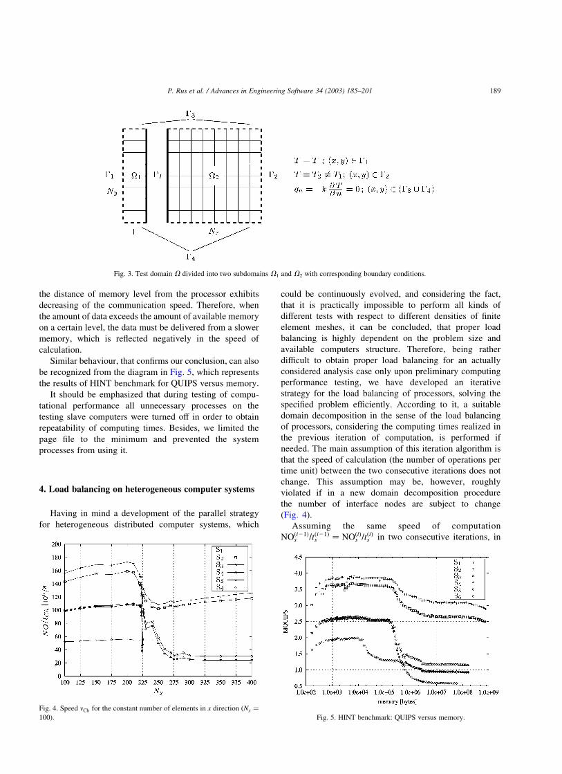
steady state heat transfer case, considering division of a

square domain into two subdomains (Fig. 3), with the

subdomain V2 being allocated to a computer whose

computational performance is to be identified.

Since a great amount of computational time in the slave

program is used for Cholesky decomposition of the matrix

Kmmss ¼ VT

s Vs; which is a symmetric banded matrix, saved in

a ‘sky-line’ form, we decided to define the speed of each

computer from the analysis of that time. The number of

floating-point operations for Cholesky decomposition can

be estimated by the equation

NOCh ¼Neð �NBW þ 1Þ2

2ð7Þ

where Ne is the number of equations corresponding to the

number of DOF of the problem, and �NBW means the half-

bandwidth of the matrix Kmmss : For a constant number of

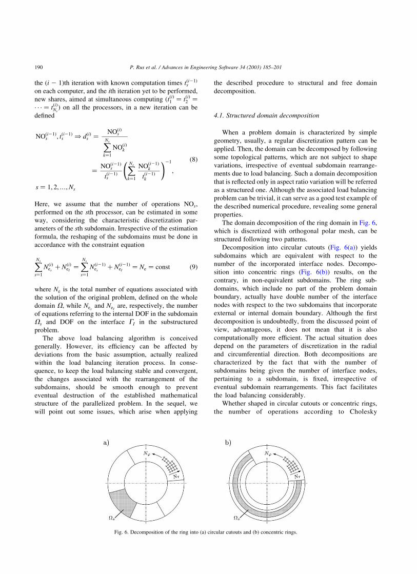
elements in the x direction ðNx ¼ 100Þ the speed of

calculation vCh; which is defined as the ratio NOCh=tCh; is

presented as a function of the problem size in Fig. 4.

Variation of the number of elements in the y direction ðNyÞ;

while Nx being fixed, has dual effect on the computation.

First, it affects the number of matrix coefficients, and

second, it affects the number of interface nodes as well.

Especially the latter, being directly associated with the

matrix bandwidth, has a tremendous role on the efficiency of

computation.

As evident from diagrams in Fig. 4 the speed of

computers S1, S2, S3, S4 and S5 decreases drastically after

a certain number of interface nodes is reached. When

inspecting for a reason of such behaviour, we found out by

analysing the program for Cholesky decomposition that

decreasing of computational speed is a direct consequence

of computer hardware structure. Actually, of the speed

of communication regarding whether processor, cache

memory or RAM is addressed. As a rule, increasing of

Table 1

Characteristics of computers in the heterogeneous distributed system

Label Type Processor RAM (MB) OS Type of program

M WS, HP B2000 PA-8000 400 MHz 1024 HP-UX 10.0 Master

S1 PC P IV 1.7 GHz 1024 WIN 2000 SP2 Slave

S2 PC P IV 1.7 GHz 1024 WIN 2000 SP2 Slave

S3 PC P III 800 MHz 256 WIN 2000 SP2 Slave




Computers are connected via Intel InBusiness 8-Port 10/100 Fast Hub.

Table 2

Benchmark of Whetstone, LINPACK and HINT and their performance

ratios

Label KIPS mflops MNetQUIPS rKIPS rmflops rMNetQUIPS

S1 0.84 169.50 55.13 1.00 1.00 1.00

S2 0.82 177.10 50.11 1.03 0.96 1.10

S3 0.68 61.54 28.76 1.24 2.75 1.92

S4 0.68 45.95 27.35 1.24 3.69 2.02

S5 0.68 45.64 27.23 1.24 3.71 2.02

S6 0.51 27.41 18.22 1.66 6.18 3.03


the distance of memory level from the processor exhibits

decreasing of the communication speed. Therefore, when

the amount of data exceeds the amount of available memory

on a certain level, the data must be delivered from a slower

memory, which is reflected negatively in the speed of

calculation.

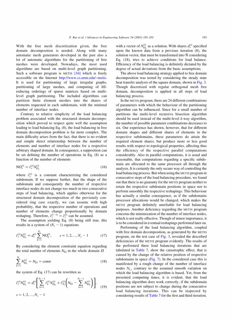
Similar behaviour, that confirms our conclusion, can also

be recognized from the diagram in Fig. 5, which represents

the results of HINT benchmark for QUIPS versus memory.

It should be emphasized that during testing of compu-

tational performance all unnecessary processes on the

testing slave computers were turned off in order to obtain

repeatability of computing times. Besides, we limited the

page file to the minimum and prevented the system

processes from using it.

4. Load balancing on heterogeneous computer systems

Having in mind a development of the parallel strategy

for heterogeneous distributed computer systems, which

could be continuously evolved, and considering the fact,

that it is practically impossible to perform all kinds of

different tests with respect to different densities of finite

element meshes, it can be concluded, that proper load

balancing is highly dependent on the problem size and

available computers structure. Therefore, being rather

difficult to obtain proper load balancing for an actually

considered analysis case only upon preliminary computing

performance testing, we have developed an iterative

strategy for the load balancing of processors, solving the

specified problem efficiently. According to it, a suitable

domain decomposition in the sense of the load balancing

of processors, considering the computing times realized in

the previous iteration of computation, is performed if

needed. The main assumption of this iteration algorithm is

that the speed of calculation (the number of operations per

time unit) between the two consecutive iterations does not

change. This assumption may be, however, roughly

violated if in a new domain decomposition procedure

the number of interface nodes are subject to change

(Fig. 4).

Assuming the same speed of computation

NOði21Þs =tði21Þ

s ¼ NOðiÞs =tðiÞs in two consecutive iterations, in

Fig. 3. Test domain V divided into two subdomains V1 and V2 with corresponding boundary conditions.

Fig. 4. Speed vCh for the constant number of elements in x direction ðNx ¼

100Þ: Fig. 5. HINT benchmark: QUIPS versus memory.


the (i 2 1)th iteration with known computation times tði21Þs

on each computer, and the ith iteration yet to be performed,

new shares, aimed at simultaneous computing ðtðiÞ1 ¼ tðiÞ2 ¼

· · · ¼ tðiÞNsÞ on all the processors, in a new iteration can be

defined

NOði21Þs ; tði21Þ

s ) dðiÞs ¼

NOðiÞsXNs

k¼1

NOðiÞk

¼NOði21Þ

s

tði21Þs

XNs

k¼1

NOði21Þk

tði21Þk

!21

;

s ¼ 1; 2;…;Ns

ð8Þ

Here, we assume that the number of operations NOs;

performed on the sth processor, can be estimated in some

way, considering the characteristic discretization par-

ameters of the sth subdomain. Irrespective of the estimation

formula, the reshaping of the subdomains must be done in

accordance with the constraint equation

XNs

s¼1

NðiÞes

þ NðiÞeI

¼XNs

s¼1

Nði21Þes

þ Nði21ÞeI

¼ Ne ¼ const ð9Þ

where Ne is the total number of equations associated with

the solution of the original problem, defined on the whole

domain V, while Nesand NeI

are, respectively, the number

of equations referring to the internal DOF in the subdomain

Vs and DOF on the interface GI in the substructured

problem.

The above load balancing algorithm is conceived

generally. However, its efficiency can be affected by

deviations from the basic assumption, actually realized

within the load balancing iteration process. In conse-

quence, to keep the load balancing stable and convergent,

the changes associated with the rearrangement of the

subdomains, should be smooth enough to prevent

eventual destruction of the established mathematical

structure of the parallelized problem. In the sequel, we

will point out some issues, which arise when applying

the described procedure to structural and free domain

decomposition.

4.1. Structured domain decomposition

When a problem domain is characterized by simple

geometry, usually, a regular discretization pattern can be

applied. Then, the domain can be decomposed by following

some topological patterns, which are not subject to shape

variations, irrespective of eventual subdomain rearrange-

ments due to load balancing. Such a domain decomposition

that is reflected only in aspect ratio variation will be referred

as a structured one. Although the associated load balancing

problem can be trivial, it can serve as a good test example of

the described numerical procedure, revealing some general

properties.

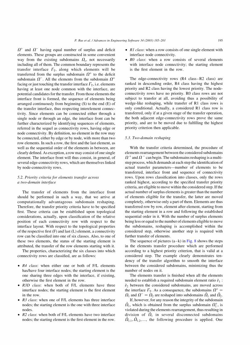
The domain decomposition of the ring domain in Fig. 6,

which is discretized with orthogonal polar mesh, can be

structured following two patterns.

Decomposition into circular cutouts (Fig. 6(a)) yields

subdomains which are equivalent with respect to the

number of the incorporated interface nodes. Decompo-

sition into concentric rings (Fig. 6(b)) results, on the

contrary, in non-equivalent subdomains. The ring sub-

domains, which include no part of the problem domain

boundary, actually have double number of the interface

nodes with respect to the two subdomains that incorporate

external or internal domain boundary. Although the first

decomposition is undoubtedly, from the discussed point of

view, advantageous, it does not mean that it is also

computationally more efficient. The actual situation does

depend on the parameters of discretization in the radial

and circumferential direction. Both decompositions are

characterized by the fact that with the number of

subdomains being given the number of interface nodes,

pertaining to a subdomain, is fixed, irrespective of

eventual subdomain rearrangements. This fact facilitates

the load balancing considerably.

Whether shaped in circular cutouts or concentric rings,

the number of operations according to Cholesky

Fig. 6. Decomposition of the ring into (a) circular cutouts and (b) concentric rings.


decomposition, Eq. (7), when applied to the subdomain

Vs; can be expressed by linear relationship

NOðiÞs ¼ cðiÞs NðiÞ

es;

cðiÞs ¼ð �NðiÞ

BWsþ 1Þ2

2¼ cði21Þ

s ¼ const

ð10Þ

Considering the above relationship in Eq. (8) and

respecting the constraint Eq. (9), a system of ðNs 2 1Þ

equations can be obtained

cðiÞs NðiÞes

¼ dðiÞs

XNs21

k¼1

cðiÞk NðiÞekþ cðiÞNs

Ne 2XNs21

k¼1

NðiÞek

!" #;

s ¼ 1; 2;…;Ns 2 1

ð11Þ

The solution of the above system is a vector of NðiÞes;

which ensures within some tolerance the required

subdomain shares dðiÞs :

For the considered ring domain, with the discretization

being defined by the corresponding number of elements in

the rðNrÞ and wðNwÞ direction, the task of load balancing is

really trivial. The number of subdomain equations NcðiÞes

¼

NðiÞes

for a circular cutout subdomain VcðiÞs can be directly

expressed in terms of the respective discretization in the w

direction. With essential boundary conditions assumed, the

following relationship is true

NcðiÞes

¼ ðNr þ 1ÞðNðiÞws2 1Þ2 2ðNðiÞ

ws2 1Þ ð12Þ

which after its resolution yields the respective number of

elements in the w direction for the considered subdomain

NcðiÞws

¼NðiÞ

es

Nr 2 1þ 1 ð13Þ

Similarly, the number of subdomain equations NrðiÞes

¼ NðiÞes

for a concentric ring subdomain VrðiÞs can be expressed in

terms of the respective discretization in the r direction as

NrðiÞes

¼ ðNðiÞrs

2 1ÞNw ð14Þ

yielding the respective number of elements in the r direction

for the considered subdomain

NrðiÞrs

¼NðiÞ

es

Nw

þ 1 ð15Þ

Because values of the vectors NcðiÞws

and NrðiÞrs

are in general in

R, they must be transformed into h considering the

constraint equations Nw ¼PNs

s¼1 NcðiÞws

and Nr ¼PNs

s¼1 NrðiÞrs

:

Due to simplicity of the considered problem, some

characteristic properties regarding load balancing can be

easily revealed by running a real physical problem. In the

sequel, results from the steady state heat transfer analysis of

the ring in Fig. 6, performed in parallel on six processors, will

be considered. The corresponding computations were per-

formed on the heterogeneous distributed system, that is

described in Table 1, and qualitatively characterized in

Table 2 and Fig. 4. On three distinct meshes ðNr £ NwÞ

considered (100 £ 1000), (1000 £ 100) and (250 £ 250),

respectively, effects of the structured domain decomposition

into circular cutouts and concentric rings on the compu-

tational efficiency were investigated. Load balancing was

performed on the slave level according to the respective load

balancing formulas (8), (11) and (13) or (15). The parameters,

that are listed in Tables 3–6, characterize dominantly a

particular computational case. Referring to a subdomain Vs

they are in turn:

Vs ! Sc allocation of the subdomain Vs to the processor Sc

Nrs;Nws

respective discretization parameters in the r and w

direction

Nesnumber of equations

NPFsprofile of the stiffness matrix

NIsnumber of interface nodes

�NBWsaverage half-bandwidth of the stiffness matrix.

Table 3

Structured domain decomposition of the ring (100 £ 1000) into circular

cutouts

Iter Vs ! Sc NwsNes

NPFsNIs

�NBWstSls

½s�

0 V1, S1 167 16,434 3,281,121 202 199 1.66

V2, S2 167 16,434 3,281,121 202 199 1.92

V3, S3 167 16,434 3,281,121 202 199 2.65

V4, S4 167 16,434 3,281,121 202 199 2.78

V5, S5 166 16,335 3,263,832 202 199 2.78

V6, S6 166 16,335 3,263,832 202 199 4.78

devðtSlÞ (%) 96.75

1 V1, S1 248 24,453 4,889,129 202 199 2.45

V2, S2 214 21,087 4,215,963 202 199 2.45

V3, S3 156 15,345 3,065,182 202 199 2.49

V4, S4 148 14,553 2,906,226 202 199 2.46

V5, S5 147 14,454 2,882,661 202 199 2.46

V6, S6 87 8,514 1,686,579 202 198 2.52

devðtSlÞ (%) 2.81

Table 4

Structured domain decomposition of the ring (1000 £ 100) into concentric

rings

Iter Vs ! Sc NrsNes

NPFsNIs

�NBWstSls

½s�

0 V1, S1 167 16,600 1,699,302 100 102 0.52

V2, S2 167 16,600 3,339,302 200 201 1.94

V3, S3 167 16,600 3,339,302 200 201 2.79

V4, S4 167 16,600 3,339,302 200 201 2.80

V5, S5 166 16,500 3,319,005 200 201 2.81

V6, S6 166 16,500 1,689,005 100 102 1.59


1 V1, S1 473 47,200 4,850,184 100 102 1.46

V2, S2 123 12,200 2,446,234 200 200 1.44

V3, S3 85 8,400 1,674,948 200 199 1.43

V4, S4 85 8,400 1,674,948 200 199 1.44

V5, S5 84 8,300 1,654,651 200 199 1.45

V6, S6 150 14,900 1,524,253 100 102 1.44

devðtSlÞ (%) 2.07


Iteration counter Iter stands for the number of iterations

needed to achieve load balance within a required tolerance.

The load balancing is performed upon realized times tSlsin the

(i 2 1)th iteration by computing the subdomain shares dðiÞs

according to Eq. (8). Time tSlsis the time of assembling the

local stiffness matrices and local loading vector, plus the time

of computing the matrix Kps and vector fps in the slave program

(Fig. 2). With devðtSlÞ; percentage of deviation from the ideal

balance is measured taking the difference between maximal

and minimal value of the time tSlsover their mean value.

As can be seen from Tables 3–6 the initial partition

was performed into six equally sized subdomains, which

resulted because of the heterogeneity of the computer system

in non-balanced computation times tSls: With the implemen-

tation of the load balancing algorithm and respective

reshaping of the subdomains from the previous iteration, the

load balanced subdomains were achieved in one further

iteration for the first two cases (Tables 3 and 4), while for the

cases presented in Tables 5 and 6 two and three iterations,

respectively, were needed. With limit of the deviation devðtSlÞ

set to5% the load balance for the first three cases was achieved

within this limit, while in the fourth case, the load balancing

procedure was stopped because of the repetition of the

respective discretization parameters in the r direction,

obviously due to not enough refined discretization.

As the (100 £ 1000) and (1000 £ 100) discretization cases

are totally equivalent with respect to the number of elements,

while considering the nature of the prescribed boundary

conditions they differ only slightly regarding the respective

numberofunknownprimaryvariables, actually99,000versus

99,900, the considered two cases are convenient for a

comparative analysis. Especially, for considering the effect

of the subdomain pattern used in the domain decomposition.

The advantage of using decomposition in concentric rings is

obvious, the reason for that, according to Eq. (7), being the

strongly reduced number of interface nodes for the two

boundary subdomains V1 and V6; respectively. The same

conclusions can be made when considering the (250 £ 250)

discretization case. Though the number of unknown primary

variables is smaller than in the former two cases, actually

62,250 versus 99,000 (or 99,900), the respective parallel

computations are considerably longer. The role of the number

of interface nodes is even more exposed. What is certainly

worth of our attention is the fact, that the processor S6, though

the worst with respect to the performed characterization

(Table 2, Fig. 4), is able to contribute significantly in the

overall computational efficiency, if only the correct sub-

domain, characterized by proper favourable discretization

properties, is allocated to it. Otherwise, the computational

performance can be spoiled tremendously.

4.2. Free domain decomposition

In most real life cases structured finite element meshes

cannot be applied, which means, that in consequence also

structured domain decomposition cannot be performed.

Table 6

Structured domain decomposition of the ring (250 £ 250) into concentric

rings

Iter Vs ! Sc NrsNes

NPFsNIs

�NBWstSls

½s�

0 V1, S1 42 10,250 2,530,627 250 246 3.14

V2, S2 42 10,250 4,968,127 500 484 11.12

V3, S3 42 10,250 4,968,127 500 484 33.23

V4, S4 42 10,250 4,968,127 500 484 34.05

V5, S5 41 10,000 4,842,380 500 484 33.33

V6, S6 41 10,000 2,467,380 250 246 4.69


1 V1, S1 111 27,500 6,894,670 250 250 8.29

V2, S2 32 7,750 3,710,657 500 478 8.57

V3, S3 11 2,500 1,069,970 500 427 9.51

V4, S4 11 2,500 1,069,970 500 427 9.75

V5, S5 11 2,500 1,069,970 500 427 9.77

V6, S6 74 18,250 4,554,531 250 249 8.39


2 V1, S1 114 28,250 7,084,411 250 250 8.51

V2, S2 32 7,750 3,710,657 500 478 8.56

V3, S3 10 2,250 9,44,223 500 419 8.77

V4, S4 10 2,250 9,44,223 500 419 8.97

V5, S5 10 2,250 9,44,223 500 419 9.01

V6, S6 74 18,250 4,554,531 250 249 7.96


3 V1, S1 112 27,750 6,957,917 250 250 8.36

V2, S2 31 7,500 3,584,910 500 477 8.31

V3, S3 10 2,250 944,223 500 419 8.77

V4, S4 9 2,000 818,476 500 409 8.18

V5, S5 9 2,000 818,476 500 409 8.19

V6, S6 79 19,500 4,870,766 250 249 8.46

devðtSlÞ (%) 6.97

Table 5

Structured domain decomposition of the ring (250 £ 250) into circular

cutouts

Iter Vs ! Sc NwsNes

NPFsNIs

�NBWstSls

½s�

0 V1, S1 42 10,209 4,946,193 502 484 10.29

V2, S2 42 10,209 4,946,193 502 484 11.05

V3, S3 42 10,209 4,946,193 502 484 33.22

V4, S4 42 10,209 4,946,193 502 484 33.98

V5, S5 41 9,960 4,761,353 502 478 32.83

V6, S6 41 9,960 4,761,353 502 478 41.54


1 V1, S1 80 19,671 9,701,988 502 493 19.24

V2, S2 75 18,426 9,018,459 502 489 19.25

V3, S3 25 5,976 2,757,809 502 461 19.83

V4, S4 25 5,976 2,757,809 502 461 20.20

V5, S5 25 5,976 2,757,809 502 461 20.35

V6, S6 20 4,731 2,191,848 502 463 20.95

devðtSlÞ (%) 8.52

2 V1, S1 82 20,169 9,952,233 502 493 19.66

V2, S2 76 18,675 9,201,480 502 492 19.69

V3, S3 25 5,976 2,757,809 502 461 19.83

V4, S4 24 5,727 2,692,692 502 470 19.86

V5, S5 24 5,727 2,692,692 502 470 20.02

V6, S6 19 4,482 2,006,447 502 447 19.39

devðtSlÞ (%) 3.20


With the free mesh discretization given, the free

domain decomposition is needed. Along with many

automatic mesh generators developed in the past also a

lot of automatic algorithms for the partitioning of free

meshes were developed. Nowadays, the most used

algorithms are based on multi-level graph partitioning.

Such a software program is METIS [16] which is freely

accessible on the Internet http://www.cs.umn.edu/~metis.

It is used for partitioning of large irregular graphs,

partitioning of large meshes, and computing of fill-

reducing orderings of sparse matrices based on multi-

level graph partitioning. The included algorithms can

partition finite element meshes into the shares of

elements requested in each subdomain, with the minimal

number of interface nodes.

Contrary to relative simplicity of the load balancing

problem associated with the structured domain decompo-

sition which proved to respect quite well the assumption

leading to load balancing Eq. (8), the load balancing in free

domain decomposition problem is far more complex. The

main difficulty arises from the fact, that there is no evident

and simple direct relationship between the number of

elements and number of interface nodes for a respective

arbitrary shaped domain. In consequence, a supposition can

be set defining the number of operations in Eq. (8) as a

function of the number of elements

NOðiÞs ¼ ~cðiÞs NðiÞ

Elsð16Þ

where ~cðiÞs is a constant characterizing the considered

subdomain. If we suppose further, that the shape of the

subdomain and consequently the number of respective

interface nodes do not change too much in two consecutive

steps of load balancing, which applies otherwise for the

structured domain decomposition of the previously con-

sidered ring case exactly, we can assume with high

probability, that the respective number of operations and

number of elements change proportionally by domain

reshaping. Therefore, ~cði21Þs ¼ ~cðiÞs can be assumed.

The assumption yielding Eq. (8) being still true, this

results in a system of ðNs 2 1Þ equations

~cðiÞs NðiÞEls

¼ dðiÞs

XNs

k¼1

NOðiÞk ; s ¼ 1; 2;…;Ns 2 1 ð17Þ

By considering the element constraint equation regarding

the total number of elements NEl in the whole domain V

XNs

k¼1

NðiÞElk

¼ NEl ¼ const ð18Þ

the system of Eq. (17) can be rewritten as

~cðiÞs NðiÞEls

¼ dðiÞs

XNs21

k¼1

~cðiÞk NðiÞ

Elkþ ~c

ðiÞNs

NEl 2XNs21

k¼1

NðiÞElk

!" #;

s ¼ 1; 2;…;Ns 2 1

ð19Þ

with a vector of NðiÞEls

as a solution. With shares dðiÞs specified

upon the known data from a previous iteration (8), the

solution vector, that must be transformed into N considering

Eq. (18), tries to achieve conditions for load balance.

Efficiency of the load balancing is definitely dictated by the

degree of actual deviations from the basic assumptions.

The above load balancing strategy applied to free domain

decomposition was tested by considering the steady state

heat transfer analysis of the square domain, shown in Fig. 3.

Though discretized with regular orthogonal mesh free

domain, decomposition is applied in all steps of load

balancing process.

In the METIS program, there are 24 different combinations

of parameters with which the behaviour of the partitioning

algorithm can be influenced. Since for a small number of

partitions the multi-level recursive bisection algorithm

should be used instead of the multi-level k-way algorithm,

the number of possible parameter combinations decreases to

six. Our experience has shown, however, that for different

domain shapes and different shares of elements in the

respective subdomains, these parameters do attain the

required element shares, but produce more or less good

results with respect to topological properties, affecting thus

the efficiency of the respective parallel computations

considerably. Also in parallel computations, it is usual and

reasonable, that computations regarding a specific subdo-

main are allocated to the same processor all through the

analysis. It is certainly the only secure way of controlling the

load balancing process. But when using the METIS program in

consecutive steps of the load balancing procedure, we found

out that there is no guaranty for the METIS program neither to

retain the respective subdomain positions in space nor to

perform smoothly the respective reshapings. This behaviour

has actually a similar consequence, as if the subdomains

processor allocations would be changed, which makes the

METIS program definitely unreliable for load balancing

purposes. Another deficiency regarding the METIS program

concerns the minimization of the number of interface nodes,

which is not really effective. Though of minor importance, it

is to be considered in eventual reshapings performed later on.

Performing of the load balancing algorithm, coupled

with free domain decomposition, as generated by the METIS

program, on the test case of Fig. 3, revealed the described

deficiencies of the METIS program evidently. The results of

the performed three load balancing iterations that are

tabulated in Table 7, show the catastrophic effect, that is

caused by the change of the relative position of respective

subdomains in space (Fig. 7). In the considered case this is

manifested by a rough change of the number of interface

nodes NIs; contrary to the assumed smooth variation on

which the load balancing algorithm is based. Yet, from the

presented computing times, it is evident, that the load

balancing algorithm does work correctly, if the subdomain

positions are not subject to change during the consecutive

load balancing iterations. This can be inspected by

considering results of Table 7 for the first and third iteration.


http://www.cs.umn.edu/~metis

Because of those facts we decided to follow a

different approach, with only initial free domain

decomposition performed by the METIS program, con-

sidering a decomposition with the minimum number of

interface nodes. For all the following rearrangements of

elements needed, due to load balance, we have developed

our own algorithm.

5. Algorithm for elements rearrangement between

subdomains

Considering the basic assumptions that were adopted in

the derivation of the load balancing algorithm Eq.(8), the

major demand on the algorithm for rearrangement of

elements between subdomains is that, the respective number

of interface nodes should change smoothly and their number

minimized as much as possible by the rearrangement of

elements. The algorithm should work for structured and free

2D quadrilateral finite element meshes.

5.1. General considerations

Let us consider two subdomains, V1 and V2; with e1

and e2 being the respective numbers of elements. If a

certain amount of elements De is rearranged between the

two subdomains, this results in formation of the new

subdomains ~V1 and ~V2; with ~e1 and ~e2 being the respective

numbers of elements. The integrity of the whole domain

being preserved, i.e. V1 <V2 ¼ ~V1 < ~V2; the identity

e1 þ e2 ¼ ~e1 þ ~e2 is true. The performed elements

rearrangement can be referred to as the subdomains

reshaping.

The most natural way of reshaping the subdomains V1

and V2 is certainly by transferring the required amount of

elements Deþ ¼ De1 . 0 from a surplus subdomain Vþ ¼

V1 to a deficit subdomain V2 ¼ V2 ðDe2 ¼ De2 ¼ 2De1Þ

over the common interface. In principle, this transfer could

be done arbitrarily, but with a risk to not attain

computational performance aimed to. Though obtaining

the demanded share of elements ~e1 and ~e2; with no

surplus/deficit element ðD~e1 ¼ D~e2 ¼ 0Þ; the efficiency of

the computation would be very probably damaged signifi-

cantly, because there is no controlled variation of the other

parameters, affecting the computation as well. In order to

fulfil the basic supposition of our approach, those par-

ameters should change sufficiently smoothly by the

elements transfer. The transfer procedure that will be

presented in the sequel is conceived in a way that, this goal

can be attained.

The number of interface nodes is no doubt the parameter

of greatest relevance. Its effect on the computation time is

multiple—it affects actually the computations performed in

parallel on the substructure level, as well as the computation

of the interface problem solution, performed by the master

computer. Considering the optimal organization of the

substructure matrices [3] the number of interface nodes can

be directly associated with the bandwidth, with quadratic

dependence on the number of operations in Cholesky

decomposition Eq. (7). Our elements transfer algorithm is

traced, so that the number of interface nodes is tried to be

minimized.

First, let us introduce some basic principles and

corresponding terminology regarding the elements transfer

operation. Whatever be the number of the subdomains, the

transfer is always performed between two subdomain groups

Table 7

Load balancing upon domain partitioning by METIS ðNEl ¼ 100; 000Þ

Vs ! Sc Iter ¼ 0 Iter ¼ 1 Iter ¼ 2 Iter ¼ 3

shElsNIs

tSlsshEls

NIstSls

shElsNIs

tSlsshEls

NIstSls

V1, S3 0.333 114 1.79 0.447 108 2.40 0.448 109 2.39 0.455 106 2.41

V2, S4 0.333 110 1.89 0.425 104 2.40 0.423 216 7.20 9.143 252 5.73

V3, S5 0.334 224 6.33 0.128 212 2.37 0.129 107 0.78 0.402 146 2.54

tSlmax6.33 2.40 7.20 5.37

Fig. 7. Subdomain space allocation according to domain partitioning by METIS.


Vþ and V2 having equal number of surplus and deficit

elements. These groups are constructed in some convenient

way from the existing subdomains Vs; not necessarily

including all of them. The common boundary represents the

transfer interface GT; along which elements will be

transferred from the surplus subdomain Vþ to the deficit

subdomain V2: All the elements from the subdomain Vþ

facing or just touching the transfer interface GT; i.e. elements

having at least one node common with the interface, are

potential candidates for the transfer. From those elements the

interface front is formed, the sequence of elements being

arranged continuously from beginning (S) to the end (E) of

the transfer interface, thus respecting interelement connec-

tivity. Since elements can be connected either through a

single node or through an edge, the interface front can be

further characterized by identifying sequences of elements,

referred in the sequel as connectivity rows, having edge or

node connectivity. By definition, no element in the row may

be connected, either by edge or by node, with more than two

row elements. In such a row, the first and the last element, as

well as the sequential order of the elements in between, are

clearly defined. As exception, a row may consist of one single

element. The interface front will thus consist, in general, of

several edge-connectivity rows, which are themselves linked

by node-connectivity rows.

5.2. Priority criteria for elements transfer across

a two-domain interface

The transfer of elements from the interface front

should be performed in such a way, that we arrive at

computationally advantageous subdomain reshaping.

Therefore, the transfer priority criteria have to be specified

first. These criteria can be established upon topological

considerations, actually, upon classification of the relative

position of each connectivity row with respect to the

interface layout. With respect to the topological properties

of the respective first (F) and last (L) element, a connectivity

row can be classified into one of six classes. Also, to one of

these two elements, the status of the starting element is

attributed, the transfer of the row elements starting with it.

The properties, characterizing the six classes into which

connectivity rows are classified, are as follows:

† R4 class: when either one or both of F/L elements

has/have four interface nodes; the starting element is the

one sharing three edges with the interface, if existing,

otherwise the first element in the row.

† R3D class: when both of F/L elements have three

interface nodes; the starting element is the first element

in the row.

† R3 class: when one of F/L elements has three interface

nodes; the starting element is the one with three interface

nodes.

† R2 class: when both of F/L elements have two interface

nodes; the starting element is the first element in the row.

† R1 class: when a row consists of one single element with

interface node connectivity.

† R0 class: when a row consists of several elements

with interface node connectivity; the starting element

is the first element in the row.

The edge-connectivity rows (R4 class–R2 class) are

ranked in descending order, R4 class having the highest

priority and R2 class having the lowest priority. The node-

connectivity rows have no priority. R0 class rows are not

subject to transfer at all, avoiding thus a possibility of

wedge-like reshaping, while transfer of R1 class rows is

only conditional. Actually, a considered R1 class row is

transferred, only if at a given stage of the transfer operation,

the both adjacent edge-connectivity rows prove the same

priority, and are to be moved due to fulfilling the highest

priority criterion then applicable.

5.3. Two-domain reshaping

With the transfer criteria determined, the procedure of

elements rearrangement between the considered subdomains

V þ andV 2 can begin. The subdomains reshaping is a multi-

step process, which demands at each step the identification of

actual transfer parameters—number of elements to be

transferred, interface front and sequence of connectivity

rows. Upon rows classification into classes, only the rows

ranked highest, according to the specified transfer priority

criteria, are eligible to move within the considered step. If the

actual number of surplus elements is greater than the number

of elements eligible for the transfer, the latter are moved

completely, otherwise only a part of them. Elements are thus

transferred row by row, element after element, starting from

the starting element in a row and following the established

sequential order in it. With the number of surplus elements

being less or equal to the number of elements eligible to move

the subdomains, reshaping is accomplished within the

considered step, otherwise another step is required with

further transfer of elements.

The sequence of pictures (a–k) in Fig. 8 shows the steps

in the elements transfer procedure which are performed

according to a highest priority criterion, that is valid at a

considered step. The example clearly demonstrates ten-

dency of the transfer algorithm to smooth the interface

between the considered subdomains, minimizing thus the

number of nodes on it.

The elements transfer is finished when all the elements

needed to establish a required subdomain element ratio ~e1 :

~e2 between the considered subdomains, are moved across

the interface GT: As a consequence, the subdomains Vþ ¼

V1 and V2 ¼ V2 are reshaped into subdomains ~V1 and ~V2:

If, however, for any reason the integrity of the subdomain

V1; which is obtained from the surplus subdomain Vþ1 ; is

violated during the elements rearrangement, thus resulting in

division of V1 in several disconnected subdomains

V1:1; V1:2;…; the following procedure is applied. One


Fig. 8. Steps in elements transfer according to transfer priority criteria.


among the subdomains V1:1; V1:2;…; having some advan-

tageous property for further reshaping, is kept, while the

others are merged in the subdomain V2: The merged

subdomainbecomes thus asurplus subdomainand the process

of elements transfer to the remainder of V1 can start again.

The described anomalous domain disintegrity is likely to

happen if a domain is not convex, or if the finite element

discretization is characterized by free meshing. In Fig. 9,

two subdomain layouts leading to this phenomenon are

shown. In both cases, the transfer of elements, if performed

sufficiently long, leads to disintegration of the initial surplus

domain into two subdomains. Considering the necessary

merging of one of them to the initial deficit domain, two

properties that are advantageous with respect to further

reshaping can be visualized. It is certainly advantageous

to merge small subdomains, retaining the largest one

(Fig. 9(a)), and to merge island-like subdomains, retaining

the boundary one (Fig. 9(b)).

5.4. Multi-domain reshaping

The rearrangement of elements in a multi-domain

follows essentially the same elements transfer procedure,

as developed for a two-domain reshaping. It is actually

performed as a multi-step operation, solving at each step a

sequence of respective two-domain reshaping problems. In

order to transform the multi-domain reshaping problem to a

two-domain reshaping problem (or a sequence of them)

the same strategy, as used by the METIS program in the

domain decomposition, is applied. There, the recursive

bisection method is applied to partition the domain V into

Ns subdomains Vs; according to the respective shares of

elements. Any subdomain VðjÞi ; arrived at after the jth

bisection step, but not reduced yet to a single subdomain

from the Vs set, is subject to further division in two

subdomains, respecting the element shares as resulting from

the respective subdomains structures. The evolution of the

partitioning process, following the described approach, can

be symbolically resumed by

V ¼ Vð1Þ1 <V

ð1Þ2 ¼ ðV

ð2Þ1 <V

ð2Þ2 Þ< ðV

ð2Þ3 <V

ð2Þ4 Þ

¼ ððVð3Þ1 <V

ð3Þ2 Þ< ðV

ð3Þ3 <V

ð3Þ4 ÞÞ< ððV

ð3Þ5 <V

ð3Þ6 Þ

< ðVð3Þ7 <V

ð3Þ8 ÞÞ

¼ · · · ¼ ðð· · ·ððV1 <V2Þ< · · · < ðVNm21

<VNmÞÞ· · ·Þ< ð· · ·ððVNmþ1 <VNmþ2Þ< · · ·

< ðVNs21 <VNsÞÞ· · ·ÞÞ ð20Þ

with Nm defined as Nm ¼ intðNs=2Þ:

The same evolution path, as established by partitioning

of the domain V, will be followed in the procedure of

rearrangement of elements in a multi-domain. First, the

subdomains Vs ðs ¼ 1;…;NmÞ and subdomains Vs ðs ¼

Nm þ 1;…;NsÞ; with respective surplus/deficit elements

Des; are merged to yield two subdomains, Vð1Þ1 and V

ð1Þ2 ;

respectively. The respective surplus/deficit elements Deð1Þ1

and Deð1Þ2 are given by

XNm

s¼1

Des ¼ Deð1Þ1 ;

XNs

s¼Nmþ1

Des ¼ Deð1Þ2 ) Deð1Þ1 þ Deð1Þ2 ¼ 0

ð21Þ

If Deð1Þ1 – 0; rearrangement of elements between the two

subdomains is needed, which is performed as described in

Fig. 9. Undesirable division of the surplus subdomain.


Section 5.3. The reshaping of the subdomains Vð1Þ1 and V

ð1Þ2

results in the subdomains ~Vð1Þ1 and ~Vð1Þ

2 ; with respective

numbers of elements ~eð1Þ1 ¼ eð1Þ1 þ Deð1Þ1 and ~e

ð1Þ2 ¼ eð1Þ2 þ

Deð1Þ2 ; and no surplus/deficit element ðD~eð1Þ1 ¼ D~eð1Þ2 ¼ 0Þ:

As a consequence of the performed subdomains Vð1Þ1 and

Vð1Þ2 reshaping, the subdomains Vs ðs ¼ 1;…NmÞ and

subdomains Vs ðs ¼ Nm þ 1;…;NsÞ are correspondingly

reshaped as well, yielding the subdomains ð1ÞVs ðs ¼

1;…;NsÞ: Because of the performed reshaping, the respect-

ive surplus/deficit elements Des; that were characterizing the

subdomains Vs ðs ¼ 1;…;NsÞ before the reshaping, are

correspondingly changed to Dð1Þes; but now fulfilling the

identities

XNm

s¼1

Dð1Þes ¼ 0;XNs

s¼Nmþ1

Dð1Þes ¼ 0 ð22Þ

The elements rearrangement process can be moved now to

the next level, in which the described rearrangement

procedure is performed separately and independently of

each other for the subdomains ~Vð1Þ1 and ~Vð1Þ

2 : Thus, the set of

subdomains ð1ÞVs ðs ¼ 1;…;NmÞ; incorporated in ~Vð1Þ1 ; is

correspondingly halved and respective subdomains

merged to yield two subdomains Vð2Þ1 and V

ð2Þ2 ; with

respective surplus/deficit elements Deð2Þ1 and Deð2Þ2 demand-

ing for the subdomains reshaping. Similarly, from the set of

subdomains ð1ÞVs ðs ¼ Nm þ 1;…;NsÞ; incorporated in ~Vð1Þ2 ;

the subdomains Vð2Þ3 and V

ð2Þ4 ; with respective surplus/deficit

elements Deð2Þ3 and Deð2Þ4 ; are obtained. The respective

reshapings of the two subdomains couples Vð2Þ1 –Vð2Þ

2 and

Vð2Þ3 –Vð2Þ

4 yield the subdomains ~Vð2Þ1 ; ~Vð2Þ

2 and ~Vð2Þ3 ; ~Vð2Þ

4 ;

with no surplus/deficit elements ðD~eð2Þ1 ¼ D~e

ð2Þ2 ¼ D~e

ð2Þ3 ¼

D~eð2Þ4 ¼ 0Þ: The respective subdomains ð1ÞVs are corre-

spondingly reshaped in the subdomain ð2ÞVs; demonstrating

Dð2Þes surplus/deficit elements. The described procedure can

be repeated, following the structure Eq. (20), until complete

fulfilment of the required element shares on the subdomains

Vs ðs ¼ 1;…;NsÞ level.

At the end, to demonstrate the general property of

the developed rearrangement algorithm—interface

smoothing and interface nodes minimization, a simple

problem is considered. When a square domain, regularly

meshed by (100 £ 100) elements, is partitioned by the

METIS program in six subdomains of the required

share (shEl1¼ shEl2

¼ shEl3¼ shEl4

¼ 0:167 and

shEl5¼ shEl6

¼ 0:166), subdomains, with a respective lay-

out as displayed in Fig. 10(a), are obtained.

Though the decomposition is performed in the sense of

minimizing the number of interface nodes, it is evident, that

the achieved number of interface nodes is not optimal. By

applying our rearrangement algorithm, however, after

execution of several reshaping of those subdomains

enforced by imposition of artificially created surplus/deficit

elements, but ending finally at the initial required shares

shEl1; shEl2

;… the subdomains layout, as displayed in

Fig. 10(b), is obtained. This layout is definitely optimal,

which proves the quality of our algorithm.

5.5. Load balancing of the square domain

Testing of computational conformity of the developed

algorithm for the rearrangement of elements, as the key

factor in load balancing, was performed on the steady state

heat transfer analysis case of the square domain in Fig. 3.

Parallel computations were performed on the same

computer system as used in the investigations of structured

domain decomposition. The respective notations introduced

there still apply, therefore, only NElsand NDEls

need be

clarified. NElsand NDEls

are the number of elements and the

number of surplus/deficit elements in each subdomain,

respectively. The respective results of the load balancing,

performed as before on the slave level, are tabulated in

Table 8.

The (300 £ 250) elements square domain was initially

partitioned into six equally sized subdomains by the METIS

program considering free domain decomposition. Actually,

the demanded shares of elements were for the first four

subdomains 0.167, and for the last two 0.166, respectively,

which was accomplished rather satisfactorily by the METIS

program. As it can be seen from Table 8, the subdomains V3

Fig. 10. Demonstration of interface smoothing and interface nodes minimization property of the developed algorithm.


Table 8

Load balancing of square domain partitioned into six subdomains

Iter Vs ! Sc NElsNes

NPFsNIs

�NBWstSls

½s� NDEls

0 V1, S5 12,490 12,362 1,918,231 230 155 1.75 22,648

V2, S4 12,599 12,477 1,984,182 237 159 1.79 22,476

V3, S1 12,631 12,473 3,691,794 404 295 5.31 3,344

V4, S6 12,385 12,261 1,953,792 237 159 2.78 639

V5, S3 12,449 12,312 1,996,895 240 162 1.88 22,028

V6, S2 12,446 12,305 3,471,697 378 282 5.09 3,169


1 V1, S5 15,138 15,006 2,504,478 250 166 2.61 279

V2, S4 15,075 14,943 2,484,410 248 166 2.52 2354

V3, S1 9,287 9,153 2,471,705 338 270 3.30 921

V4, S6 11,746 11,627 1,787,372 232 153 2.50 2325

V5, S3 14,477 14,358 2,337,727 243 162 2.24 21,286

V6, S2 9,277 9,139 2,416,896 343 264 3.49 1,123


2 V1, S5 15,217 15,086 2,500,464 249 165 2.51 2570

V2, S4 15,429 15,299 2,569,331 250 167 2.65 2137

V3, S1 8,366 8,234 2,171,144 329 263 2.85 211

V4, S6 12,071 11,951 1,845,611 234 154 2.59 2249

V5, S3 15,763 15,642 2,657,118 254 169 2.85 422

V6, S2 8,154 8,020 2,057,456 326 256 2.93 323


3 V1, S5 15,787 15,655 2,661,782 255 170 2.91 474

V2, S4 15,566 15,433 2,614,834 252 169 2.75 43

V3, S1 8,155 8,022 2,139,848 329 266 2.86 178

V4, S6 12,320 12,201 1,907,414 232 156 2.67 2149

V5, S3 15,341 15,223 2,527,548 250 166 2.52 2652

V6, S2 7,831 7,699 1,980,058 322 257 2.81 105


4 V1, S5 15,312 15,181 2,548,529 250 167 2.65 2363

V2, S4 15,523 15,394 2,585,794 251 167 2.69 2248

V3, S1 7,977 7,847 2,050,285 323 261 2.66 2174

V4, S6 12,469 12,349 1,945,402 233 157 2.74 282

V5, S3 15,993 15,871 2,709,616 256 170 3.06 741

V6, S2 7,726 7,592 1,988,878 325 261 2.87 126


5 V1, S5 15,675 15,543 2,642,529 253 170 2.84 325

V2, S4 15,771 15,638 2,659,097 254 170 2.86 380

V3, S1 8,151 8,018 2,144,592 329 267 2.84 169

V4, S6 12,551 12,432 1,920,845 232 154 2.68 2100

V5, S3 15,252 15,134 2,510,315 249 165 2.52 2610

V6, S2 7,600 7,468 1,891,993 323 253 2.61 2163


6 V1, S5 15,351 15,221 2,536,140 250 166 2.62 2340

V2, S4 15,391 15,261 2,557,027 251 167 2.65 2250

V3, S1 7,982 7,852 2,052,093 323 261 2.65 2130

V4, S6 12,651 12,530 1,993,434 235 159 2.82 187

V5, S3 15,862 15,740 2,672,029 255 169 2.85 315

V6, S2 7,763 7,629 2,007,068 326 263 2.90 218


7 V1, S5 15,691 15,560 2,630,145 252 169 2.80 69

V2, S4 15,641 15,508 2,628,058 253 169 2.77 20

V3, S1 8,112 7,979 2,125,741 329 266 2.81 68

V4, S6 12,464 12,345 1,939,155 232 157 2.72 260

V5, S3 15,547 15,428 2,610,970 252 169 2.73 293

V6, S2 7,545 7,413 1,928,996 322 260 2.76 24

devðtSlÞ (%) 3.25


and V6 have more interface nodes than other subdomains,

therefore, we allocated the most powerful computers (S1 and

S2) to them. As expected, due to heterogeneity of the

distributed system, the computing times tSlswere not load

balanced. By applying in continuation of the computational

analysis, load balancing according to the developed

algorithm implemented by our element transfer algorithm,

the load balance between the subdomains were achieved in

seven iterations.

6. Conclusion

Several issues regarding parallel computations on a

system of heterogeneous distributed computers were

addressed in the paper, the parallelization being performed

upon domain decomposition approach and finite element

substructuring method.

Despite performing different standard benchmarks to

characterize the computational performance of hetero-

geneous components, this proved, though qualitatively

correct, insufficient for realistic characterization, in particu-

lar, with respect to large finite element systems considered.

By analysing structure of the substructuring method and

revealing the most influential parameters affecting the speed

of computation, we arrived at the conclusion to develop

specific self-adjusting algorithms to cope with the problem,

irrespectively of the problem size and heterogeneity of the

computer system.

To optimize the computational performance in parallel

by even distribution of the work among the processors,

proper load balancing is needed. A load balancing

algorithm, based on the assumption of preserving the

speed of computation in the consecutive iterations, is

developed. Irrespective of the subdomains size and

processors performance, it can determine upon computing

times realized in the previous computing step, shares needed

for a balanced computation. The efficiency of the algorithm

is first demonstrated on cases allowing structured domain

decomposition. When using the algorithm in relation to free

domain decomposition, based on the use of the partitioning

METIS program, several deficiencies of the latter tend to

spoil the efficiency of the developed load balancing

algorithm. Therefore, an algorithm for reshaping of the

existing subdomains in accordance with the required shares

is developed. The rearrangement of elements between

subdomains is performed in a way that assumptions used

in the derivation of the load balancing algorithm are

respected as much as possible. This includes above all

smooth shape variations and minimization of the respective

interface nodes.

Considering the majority of non-linear solvers contain-

ing a linear solution step presenting almost always the

predominant source of CPU time consumption, the used

approach and the algorithms developed cope quite well also

with this class of problems. In fact, when the whole

investigated domain is subject to non-linear effects, such as

in metal forming processes that are characterized by large

plastic deformation through the entire domain, it is not

expected that computational efficiency in parallel would be

spoiled considerably, namely, the load balancing, which

relies on the time needed for the formation of the respective

subproblem matrices and corresponding computations prior

to the solution of the interface problem, will perform quite

well in computations where a small number of iterations is

needed to attain convergence within an incremental step.

The eventual increase of the number of iterations would

definitely spoil the computational efficiency in parallel to

what extent it depends on the properties of the considered

problem. In such cases, if appropriate, the basis on which

the load balance is performed can be changed at will, which

again can be successfully covered by the same developed

algorithms. If, on the contrary, only a minor subdomain is

characterized by a non-linear response, such as in elasto-

plastic problems with only a part of the whole domain being

plastically deformed, this definitely causes the components

allocated to the subdomains exhibiting elastic behaviour to

be idle, while components performing the needed recalcula-

tions on the plastic subdomains being busy. Eventual

temptations to rearrange the established domain decompo-

sition are not justified since they would spoil the

performance of that part of the computation, i.e. the system

of equations solution, which is timely dominant.

Both developed algorithms enable efficient parallel

computing on heterogeneous distributed systems. Also, it

is not necessary to know the performance characteristics of

the new added computers to the existing distributed system,

because the load balancing algorithm adapts the allocated

work to the disposable computational power directly during

the computation.

References

[1] Bittnar Z, Kruis J, Nemecek J, Patzak B, Rypl D. Parallel and

distributed computations for structural mechanics: a review. In:

Topping B, editor. Civil and structural engineering computing.

Stirling, UK: Civil-Comp Press; 2001.

[2] Keyes DE. Domain decomposition in the mainstream of compu-

tational science. Proceedings of the 14th International Conference on

Domain Decomposition Methods in Cocoyoc, Mexico; 2002.

[3] Doltsinis IS, Nolting S. Generation and decomposition of finite

element models for parallel computations. Comput Syst Engng 1991;

2(5/6):427–49.

[4] Farhat C, Wilson E, Powell G. Solution of finite element systems on

concurrent processing computers. Engng Comput 1987;2(3):157–65.

[5] Kocak S, Akay H. Parallel Schur complement method for large-scale

systems on distributed memory computers. Appl Math Modell 2001;

25:873–86.

[6] Roux F, Farhat C. Parallel implementation on the two-level FETI

method. Proceedings of the 11th International Conference on Domain

Decomposition Methods in Greenwich, England; 1998.

[7] Hribersek M, Kuhn G. Domain decomposition methods for conjugate

heat transfer computations by BEM. Fifth World Congress on

Computational Mechanics, Vienna, Austria; 2002.


[8] Khan AI, Topping BHV. Parallel finite element analysis using Jacobi-

conditioned conjugate gradient algorithm. Adv Engng Software 1996;

25:309–19.

[9] Silva LM. Number-crunching with Java applications. Proc Int Conf

Parallel Distrib Process Tech Appl 1998;379–85.

[10] Labriaga R, Williams D. A load balancing technique for hetero-

geneous distributed networks. Proceedings of the International

Conference on Parallel and Distributed Processing Techniques and

Applications; 2000.

[11] Bohn CA, Lamont GB. Load balancing for heterogeneous clusters of

PCs. Future Gener Comput Syst 2002;18:389–400.

[12] Darcan O, Kaylan R. Load balanced implementation of standard clock

method. Simul Practice Theor 2000;8:177–99.

[13] Diekmann R, Preis R, Schlimbach F, Walshaw C. Shape-optimized

mesh partitioning and load balancing for parallel adaptive FEM.

Parallel Comput 2000;26:1555–81.

[14] Decker T, Luling R, Tschoke S. A distributed load balancing

algorithm for heterogeneous parallel computing system. Proc Int

Conf Parallel Distrib Process Tech Appl 1998;933–40.

[15] Lingen FJ. A versatile load balancing framework for parallel

applications based on domain decomposition. Int J Numer Meth

Engng 2000;49:1431–54.

[16] Karypis G, Kumar V. A software package for partitioning unstruc-

tured graphs, partitioning meshes, and computing fill-reducing

orderings of sparse matrices. University of Minnesota, Department

of Computer Science/Army HPC Research Center Minneapolis; 1998.

URL: http://www.cs.umn.edu/~karypis.

[17] Geist A, Beguelin A, Dongarra J, Jiang W, Manchek R, Sunderam V.

PVM: parallel virtual machine, a users’ guide and tutorial for

networked parallel computing. Cambridge: The MIT Press; 1994.

[18] Double Precision Whetstone, ORNL. URL: http://www.netlib.org/

benchmark/whetstoned.

[19] Dongarra J. Performance of various computers using standard linear

equations software in a Fortran environment, ORNL, update

periodically. URL: http://www.netlib.org/benchmark/performance.ps.

[20] Gustafson JL, Snell QO. HINT: a new way to measure computer

performance, scalable computing laboratory, Ames Laboratory. URL:

http://www.scl.ameslab.gov/Projects/HINT/index.html.


http://www.cs.umn.edu/~karypis

http://www.netlib.org/benchmark/whetstoned

http://www.netlib.org/benchmark/whetstoned

http://www.netlib.org/benchmark/performance.ps

http://www.scl.ameslab.gov/Projects/HINT/index.html

parallel computing with load balancing on heterogeneous distributed systems

Documents