parallel computing algorithms for tandem mass spectrum analysis
TRANSCRIPT

PARALLEL COMPUTING ALGORITHMS FOR TANDEM
MASS SPECTRUM ANALYSIS
A Thesis Submitted to the College of
Graduate Studies and Research
In Partial Fulfillment of the Requirements
For the Degree of Master of Science
In the Division of Biomedical Engineering
University of Saskatchewan
Saskatoon
By
Jian Sun
Copyright Jian Sun, July, 2013. All Rights Reserved

i
PERMISSION TO USE
In presenting this thesis in partial fulfilment of the requirements for a Postgraduate degree from the University of Saskatchewan, I agree that the Libraries of this University may make it freely available for inspection. I further agree that permission for copying of this thesis in any manner, in whole or in part, for scholarly purposes may be granted by the professor or professors who supervised my thesis work or, in their absence, by the Head of the Division or the Dean of the College in which my thesis work was done. It is understood that any copying or publication or use of this thesis or parts thereof for financial gain shall not be allowed without my written permission. It is also understood that due recognition shall be given to me and to the University of Saskatchewan in any scholarly use which may be made of any material in my thesis. Requests for permission to copy or to make other use of material in this thesis in whole or part should be addressed to:
Head of the Division of Biomedical Engineering
57 Campus Drive
University of Saskatchewan
Saskatoon, Saskatchewan
Canada
S7N 5A9

ii
ABSTRACT
Tandem mass spectrometry, also known as MS/MS, is an analytical technique to measure the
mass-to-charge ratio of charged ions and widely used in genomics, proteomics and
metabolomics areas. There are two types of automatic ways to interpret tandem mass spectra:
de novo methods and database searching methods. Both of them need to use massive
computational resources and complicated comparison algorithms. The real-time
peptide-spectrum matching (RT-PSM) algorithm is a database searching method to interpret
tandem mass spectra with strict time constraints. Restricted by the hardware and architecture
of an individual workstation the RT-PSM algorithm has to sacrifice the level of accuracy in
order to provide prerequisite processing speed. The peptide-spectrum similarity scoring
module is the most time-consuming part out of four modules in the RT-PSM algorithm, which
is also the core of the algorithm.
In this study, a multi-core computing algorithm is developed for individual workstations.
Moreover, a distributed computing algorithm is designed for a cluster. The improved
algorithms can achieve the speed requirement of RT-PSM without sacrificing the accuracy.
With some expansion, this distributed computing algorithm can also support different PSM
algorithms. Simulation results show that compared with the original RT-PSM, the
parallelization version achieves 25 to 34 times speed-up based on different individual
workstations. A cluster with 240 CPU cores could accelerate the similarity score module 210

iii
times compare with the single-thread similarity score module and the whole peptide
identification process 85 times compare with the single-thread peptide identification process.
Keywords: real-time peptide-spectrum matching (RT-PSM) algorithm, tandem mass spectrum,
parallel computing algorithm, multi-core computing algorithm, distributed computing
algorithm, peptide identification

iv
ACKNOWLEDGEMENTS
I would like to express my sincere appreciation to my supervisor Dr. FangXiang Wu for
supporting me over my study and research, and for their encouragement and guidance
throughout my M.Sc. program.
I would like to thank my advisory committee members Dr. Chris Zhang and Dr. Tony Kusalik
for their guidance and support.
I would like to specially thank my lab-mate Bolin Chen for his valuable comments,
suggestions, and discussions.
I would like to express my deepest gratitude to my family for all of their support and love.

v
CONTENTS
PERMISSION TO USE .................................................................................................. i
ABSTRACT ................................................................................................................... ii
ACKNOWLEDGEMENTS .......................................................................................... iv
CONTENTS ................................................................................................................... v
LIST OF TABLES ....................................................................................................... vii
LIST OF FIGURES ................................................................................................... viii
LIST OF ABBREVIATIONS ....................................................................................... ix
CHAPTER 1 INTRODUCTION ................................................................................... 1
1.1 Background .............................................................................................................. 1
1.1.1 Tandem mass spectrometry ............................................................................... 1 1.1.2 Peptide identification ......................................................................................... 2 1.1.2 De novo sequencing and database searching .................................................... 5
1.2 Motivation and Objectives ....................................................................................... 8
1.2.1 Motivation ......................................................................................................... 8 1.2.1 Objectives .......................................................................................................... 9 1.2.3 Thesis overview ............................................................................................... 12
CHAPTER 2 RT-PSM: A REAL-TIME PEPTIDE-SPECTRUM MATCHING ALGORITHM.............................................................................................................. 13
2.1 Introduction ............................................................................................................ 13
2.2 Function Modules of RT-PSM ............................................................................... 15
2.2.1 Experimental spectrum processing module ..................................................... 15 2.2.2 Candidate peptides selection module .............................................................. 16 2.2.3 Similarity score module ................................................................................... 17 2.2.4 Statistical significance computation module ................................................... 20
2.3 Performance Analysis of RT-PSM ......................................................................... 23
CHAPTER 3 RT-PSM WITH PARALLEL PROGRAMMING .................................. 26
3.1 Overall of Parallel Computing Technology ........................................................... 26
3.2 SIMD vs Multi-Core Computing ........................................................................... 27
3.3 Database vs Datastore ............................................................................................ 32
3.3.1 The advantages of SQL database ..................................................................... 32 3.3.2 The shortages of SQL database ....................................................................... 34
3.4 Algorithm and Implementation .............................................................................. 35

vi
3.4.1 Parallel programming design pattern .............................................................. 36 3.4.2 Parallel function selection ............................................................................... 38 3.4.3 Thread affinity ................................................................................................. 40 3.4.4 General code optimization ............................................................................... 41 3.4.5 Algorithm ......................................................................................................... 42
CHAPTER 4 RT-PSM WITH DISTRIBUED PROGRAMMING .............................. 45
4.1 Introduction ............................................................................................................ 45
4.1.1 Distributed computing and cluster .................................................................. 45 4.1.2 WINDOWS HPC library ................................................................................. 46
4.2 Methodology .......................................................................................................... 50
CHAPTER 5 MULTIDIMENSIONAL SEARCH: SPEED-UP PEPTIDE DATABASE SEARCHING ............................................................................................................... 54
CHAPTER 6 EXPERIMENTAL RESULTS AND DISCUSSION ............................. 57
6.1 Experimental Environment and Datasets ............................................................... 57
6.2 Verification ............................................................................................................. 58
6.3 Peptide Database Search Speed-up ........................................................................ 59
6.4 Multithread RT-PSM Performance ........................................................................ 60
6.5 Distributed Computing RT-PSM (DC RT-PSM) Performance .............................. 62
6.5 Discussions ............................................................................................................ 65
CHAPTER 7 CONCLUSIONS AND FUTURE WORK ............................................ 67
7.1 Conclusions ............................................................................................................ 67
7.2 Future Work ........................................................................................................... 68
REFERENCES ............................................................................................................ 69

vii
LIST OF TABLES
2.1 Types and 𝑚/𝑧 values of fragment ions .......................................................................... 18
2.2 Profile report for RT-PSM .................................................................................................. 26
6.1 Cluster hardware specification ........................................................................................... 57
6.2 Result comparison between MT RT-PSM and original RT-PSM ...................................... 58
6.3 Result comparison between linear search and 2-demensional search ............................... 59
6.4 Experiment hardware environment information ................................................................ 59

viii
LIST OF FIGURES
1.1 A typical proteomic mass spectrometric experiment can be divided into five steps ......... 2
1.2 The fragmentation of a peptide by CID ............................................................................... 3
1.3 A typical tandem mass spectrum consists of many peaks .................................................... 4
2.1 The workflow illustrates the process of tandem mass spectrum identification in RT-PSM ............................................................................................................................. 23
2.2 Profiling results of RT-PSM indicates that the computation of the similarity scores consumes the most CPU time ........................................................................................... 25
3.1 SIMD: each processing can operate on a different data element with the same instruction at any given clock cycle ........................................................................................................... 29 3.2 General classifications of parallel algorithms .................................................................... 37 3.3 Windows scheduler simultaneously starts 4 threads of MT RT-PSM in 4 cores ............... 41 3.4 The flowchart illustrates the process of a multi-core computing algorithm in MT RT-PSM ............................................................................................................................. 43 4.1 The flowchart illustrates Microsoft compute cluster architecture ...................................... 47 4.2 The flowchart illustrates the job scheduler architecture..................................................... 48 4.3 The flowchart illustrates the job life cycle ......................................................................... 49 4.4 The flowchart illustrates the process of a distributed computing algorithm in DC RT-PSM ............................................................................................................................. 52 5.1 2-Dimensional peptide database structures in contrast of original peptide database structure............................................................................................................................. 54 6.1 Speed-up of execution time for MT RT-PSM benchmark to original RT-PSM in 4 experiment computers ....................................................................................................... 59 6.2 Speed-up of execution time for MT RT-PSM benchmark to single thread MT RT-PSM in 4 experiment computers ....................................................................................................... 60 6.3 Speed-up of similarity scoring module execution time for DC RT-PSM benchmark to single thread MT RT-PSM from experiment dataset A (blue line) and experiment dataset B (red line) ................................................................................................................................... 62 6.4 Speed-up of execution time for DC RT-PSM benchmark to single thread MT RT-PSM from experiment dataset A (blue line) and experiment dataset B (red line) ........................... 63

ix
LIST OF ABBREVIATIONS
CCP Compute Cluster Pack CID Collision-Induced Dissociation DC RT-PSM Distributed Computing Real-Time Peptide-Spectrum Matching FIFO First In First Out HT Hyper-Threading Technology MFC Microsoft Foundation Class Library MPI Message Passing Interface MS Mass Spectrum MS/MS Tandem Mass Spectrometry MT RT-PSM Multiple Core Real-Time Peptide-Spectrum Matching NNS Nearest Neighbor Search PSM Peptide-Spectrum Matching PVM Parallel Virtual Machine RAM Random-Access Memory RT-PSM Real-Time Peptide-Spectrum Matching SIMD Single-Instruction Multiple-Data SQL Structured Query Language SSE Streaming SIMD Extension UI User Interface
1
CHAPTER 1
INTRODUCTION
1.1 Background
1.1.1 Tandem mass spectrometry
Proteomics is a significant study field in the early detection of disease, chemical
analysis and the pharmaceutical industry. One of the most important goals in
proteomics is to identify and characterize the proteins and protein complexes present
in cells grown under various conditions. Tandem mass spectrometry (MS/MS) is a
very important tool for this purpose.
A mass spectrometer separates ions according to their mass-to-charge ratio (𝑚/𝑧), and
records the relative abundance of each ionic species present [1]. Tandem mass
spectrometry consists of two mass spectrometers connected in series. In proteomics,
MS/MS is particularly used in determining the protein components of complex
mixtures. The workflow of a proteomic mass spectrometric experiment mainly
contains the five following steps. In the first step, proteins which need to be identified
are extracted from experiment substances (cell/tissue) through biochemical
fractionation and the sample complexity is reduced via polyacrylamide gel
electrophoresis (1D- or 2D-PAGE). In the second step, the protein mixture is digested
into peptides with suitable sizes by using site-specific proteases. In the third step, the

2
peptides are separated by using reversed-phase high-performance liquid
chromatography (RP-HPLC) before being placed into the mass spectrometer. In the
fourth step, peptides are ionized via electrospray ionization. The first mass
spectrometer of MS/MS captures and detects the mass spectra of the peptide ions
(MS). Then the MS with highest relative intensity will be selected to process in next
step. In the last step, the selected peptides are fragmented again by collision-induced
dissociation (CID). The second mass spectrometer in the series scans the fragments
and collects the mass spectra of fragment ions, which are called tandem mass spectra
[2]. For more details about tandem mass spectrometers, please refer to [3].
Figure 1.1 A typical proteomic mass spectrometric experiment can be divided into five steps [2]
1.1.2 Peptide identification
Generally, peptides can be identified through their small fragmentations in a mass
spectrometer. Peptides can be fragmented into pieces at their peptide bond. A piece
which contains information and which can be used to identify this peptide in a protein
Sample cell/tissue
Step 1: 1D/ 2D-PAGE
Step 2: Site-specific proteases
Step 3: RP-HPLC
Step 4: MS1
Step 5: MS2
Computer
Protein mixture Peptides
MS spectrum Tandem mass spectrum

3
database is called a peptide sequence tag. The common peptide fragment ions belong
to two different groups: N-terminal and C-terminal. The end of the polypeptide
terminated by an amino acid carboxyl group (-COOH) is called the C-terminal. The
start of the polypeptide terminated by an amino acid amine group (-NH2) is called the
N-terminal. Figure 1.2 represents the fragmentation of a precursor peptide ion by CID.
The breakages mainly occur in three different kinds of sites along the peptide
backbone: CH-CO, CO-NH and NH-CH bonds. Therefore, there are six types of
fragment ions in a fragment ion spectrum. If the N-terminal of a fragment ion keeps a
charge, this ion is classified as an a- ion, b- ion or c-ion; if the C-terminal of fragment
ion keeps a charge, this ion is classified as a x- ion, y- ion or z-ion [4].
Figure 1.2 The fragmentation of a peptide by CID [4]
These six kinds of ions might lose 𝑘 ammonia and/or water molecules. Hence, there
are (𝑘 + 1)(𝑘 + 2)/2 possible ions. 𝑘 represents the length of the peptide
fragmentation sequence. However, if the precursor ion carries multiple positive
charges, those ions could also carry more positive charges. Therefore, if a peptide

4
consists of 𝑛 amino acids and carries 𝑗 charges, its theoretical spectrum [5] might
have 3 × 𝑛 × 𝑗 × (𝑘 + 1)(𝑘 + 2) ion peaks [6, 7]. In practice, only a few of
those components are thermodynamically favored in CID reactions. In addition, due
to the limitation of resolution and sensitivity of mass spectrometers, some fragment
ions might be filtered. As a result, most (if not all) experimental spectra contain far
fewer ion peaks than their corresponding theoretical spectra.
Peptide-spectrum matching (PSM) is an operation involving an experimental
spectrum (Se) and the theoretic spectrum (Sp) of a peptide P. If a certain number of
𝑚/𝑧 values of an experimental spectrum are approximately similar with those of a
theoretical spectrum, then the experimental spectrum could be judged to have been
produced from the peptide corresponding to this theoretical spectrum.
Figure 1.3 A typical tandem mass spectrum consists of many peaks (modified from [8])

5
1.1.2 De novo sequencing and database searching
The tandem mass spectral data is the elemental resource in a peptide identification
procedure. The identification procedure is mainly performed in computers through
peptide identification programs. There are two main ways in which tandem mass
spectra are used to identify peptides, known as database searching and de novo
(peptide) sequencing.
De novo (peptide) sequencing is a process that derives a peptide’s amino acid
sequence from its tandem mass spectrum without the assistance of a sequence
database [9]. The main idea of de novo sequencing is to compare the mass difference
between two fragment ions in order to calculate the mass of an amino acid residue on
the peptide backbone. In the spectrum, if either the y-ion or b-ion series could be
identified, the peptide sequence can be determined.
There are several different algorithms based on the de novo sequencing principle in
research and industrial fields, and most successful ones have three common factors.
Sequencing errors or nucleotide polymorphisms decrease the accurate rate of peptide
identification. The first factor is good sample preparation and high quality sequencing
machine. They can provide high quality experimental data to reduce the negative
effects of sequencing errors. The second factor is an efficient matching method which
is capable of quickly identifying the common part of two different fragments. The
third is an accurate assembly algorithm to process repeated sequences [10]. In

6
addition to the previous factors, the method can be negatively affected by factors such
as incorrect assignments of y-ions or b-ions, missing fragment ion information, the
noise peaks in the spectrum, etc. The biggest advantage of de novo sequencing is that
it does not need the assistance of a sequence database. Due to this unique
characteristic, de novo sequencing still is an efficient way to identify unknown
peptides. A number of algorithms and software packages have been developed using
this approach, such as PEAKS, PepNovo and Lutefisk [10].
The limitations of de novo sequencing methods are also obvious. It requires an
extraordinary amount of computation time to successfully solve for peptide
identification. Sometimes the peptide cannot be identified directly by de novo
methods. Then the calculated result needs to be analyzed by human experts.
Compared with de novo sequencing, database searching is a much quicker
methodology. In this method, the experimental spectra are compared to the theoretical
spectra of peptides in a database. The results are statistically analyzed to find the best
match. Although the database searching still requires massive computational resources,
compared to the de novo method, this methodology eliminates numerous computation
workloads and rapidly improves the matching speed. The obvious disadvantage of
database searching is that the peptide sequence to be identified has to be in the peptide
database, because otherwise the algorithm cannot identify it. Another problem is that
the risk of false positives increases with a smaller database. The peptide database is

7
derived from a protein database. There are research institutions such as UniProt [11],
which continuously publish immense and accuracy-verified protein databases in
different research fields. With those increasing gigantic protein databases, this
shortage could be remedied. In most circumstances, the unknown peptides can be
identified with these protein databases.
In the database searching methodology, the scoring function is the core module. It
represents the similarity between an experimental spectrum and a theoretical spectrum
which is derived from the peptide database. If a score is above a confidence threshold,
it is called a hit. Undoubtedly, a good scoring function can increase the identification
accuracy and is an important factor for peptide identification. There are several
commercial or open-source software packages using database searching algorithms,
notably SEQUEST [6], MASCOT [7], and X!tandem [12]. SEQUEST uses
cross-correlation to do further similarity comparisons to generate the output.
X!Tandem and MASCOT use probability-based scoring schemes.
With the improvement of database systems and the spectra quality filter algorithms,
researchers have developed and implemented a real-time control methodology for
efficiently identifying the peptide in the process of tandem mass spectral data
acquisition, called a real-time peptide-spectrum matching (RT-PSM) algorithm.
Machine learning methods and neural network could be employed to construct the
classifier (as the quality assessor) which discriminates the high quality spectra from

8
the poor ones. In addition, with the modern database searching algorithm, searching a
large size database is also very efficient. All these technologies present an opportunity
to improve RT-PSM algorithms and implementations.
1.2 Motivation and Objectives
1.2.1 Motivation
Over the past decades, there has been an explosion in the size of protein databases due
to the technological improvement of mass spectrometry [13]. Furthermore,
researchers in proteomics wish to implement a real-time peptide identification
algorithm to improve identification procedure performance.
Dr. Wu et al. proposed a new RT-PSM procedure and the key component is "Identify
Peptide by a fast algorithm" which is performed by a software application [5]. The
original PSM procedure does not include any external software controlling feature.
This new procedure uses the software controlling module to accelerate the peptide
identification procedure.
As a real-time system, the time window of each peptide identification procedure is
limited by the spectra acquiring time of mass spectrometers [5]. Practical experiments
indicate that Wu et al.’s RT-PSM algorithm cannot completely satisfy the real-time
system requirement. Using parallel computation to improve the speed of

9
peptide-spectrum matching can be an effective method to solve this problem. Duncan
et al. use a workstation cluster as a platform to develop the "Parallel Tandem" [12].
Parallel Tandem consists of the database search, X!Tandem, and a Linux cluster
environment with Parallel Virtual Machine (PVM) or Message Passing Interface (MPI)
installed. A second example is the parallel version of SEQUEST [14], which is also
based on a PVM in a cluster environment. Another design uses the SIMD instructions
of either modern CPUs or graphical processing units (GPUs) in a single workstation
as a platform [13, 15]. Use of the SIMD instructions can result in better performance
than original RT-PSM algorithm. Most systems leveraging SIMD processing are
based on the NVIDIA's CUDA environment [15].
No matter whether a cluster environment or CUDA is used, the principles of parallel
computing are identical: dividing a large sequential process into several independent
sub-processes and executing the sub-processes concurrently to reduce execution time.
However, the previous parallel computing methodologies for analyzing tandem mass
spectra all have shortcomings. X!Tandem and SEQUEST use peptide-spectrum
matching algorithms which are slower than the RT-PSM algorithm [5] for processing
a single spectrum. SIMD and CUDA have strict hardware restrictions. SIMD
instructions are restricted by the CPU L2 Cache [16] and CUDA can only support
NVIDIA's video card. As a result, the parallel matching programs based on CUDA
have to use a powerful graphics card from NVIDIA Company.

10
1.2.1 Objectives
It is not a trivial task to improve the performance of an existing system. All
improvements should be based on the existing system and not violate any assumptions
or affect system results. The ultimate goal of this study is to develop and implement
faster peptide-spectrum matching algorithms based on the existing RT-PSM by using
parallel computing techniques. The improved algorithms should not reduce the
identification accuracy. The main idea is to design a distributed computing platform
and using the platform to parallelize the existing RT-PSM algorithms, and rapidly
accelerate the peptide identification procedure by using multiple CPUs to calculate
concurrently. To achieve the ultimate goal, four specific objectives are defined as
follows.
Objective 1: Refactor the existing RT-PSM algorithm and reduce the redundancy and
inefficiencies. The original RT-PSM design and source code were developed several
years ago. With the improvement of design patterns and development environments,
the original design could be refactored to make it more robust. Replacing the obsolete
functions and adjusting the unnecessary or redundant functions can improve the
performance in certain level.
Objective 2: Develop and implement a multithread RT-PSM algorithm in a multi-core
CPU environment. The original RT-PSM was designed to work in a single-CPU
workstation, and there was no optimization for multithreaded computation. The

11
implementation of a parallel computing algorithm for the RT-PSM in a standalone
workstation is the fundamental step of this study. The speed-up of the multithread
version of RT-PSM also is one of the benchmarks performed in this study.
Objective 3: Develop and implement a distributed RT-PSM algorithm in a distributed
computing environment, i.e. a cluster. The structure of a distributed computer is
different from the standalone workstation, so the distributed computing algorithm also
needs to be redesigned by using a different design pattern. The distributed computing
platform should be able to manage a large number of computing tasks concurrently
and the distributed version of RT-PSM should provide great performance
improvement.
Objective 4: Improve the peptide database searching algorithm to perform the
searches in constant time independent of the size of the database. The original
RT-PSM employs a traditional linear database searching algorithm. The computational
complexity of the searching algorithm highly depends on the scale of the database.
With the continuously increasing protein database, the performance of this searching
algorithm could become a bottleneck of the whole system. In this study, an advanced
database searching algorithm will be involved and the time complexity of the new
searching algorithm should be independent of the size of the database. The
experimental results also will be provided to display whether the new searching
algorithm fits with the multithread system.

12
Though this study have been designed and developed on RT-PSM, they also can be
applied to other database searching software packages with limited modifications.
Alternatively, the distributed computing algorithm also can be applied to other peptide
matching methods. Hence, this study not only creates a high-speed version
of RT-PSM, but also establishes a generic distributed computing platform. This
platform should be compatible with different peptide identification algorithms and
provide them with speed-ups on clusters.
1.2.3 Thesis overview
In this thesis, the problems of the existing RT-PSM algorithm are described and a new
design by using parallel computing algorithms is proposed. As this implementation is
based on RT-PSM, an introduction of the design and workflow of RT-PSM are given
in Chapter 2. The performance profiling results and core function analysis are also
given in Chapter 2. Chapter 3 provides a method to parallelize the critical peptide
matching function by using a multi-core computing algorithm. This method is
implemented in a standalone workstation. The distributed computing algorithm for the
cluster is presented in the Chapter 4. Chapter 5 displays the multidimensional peptide
database searching algorithm while Chapter 6 lists all experimental results which
include the experimental environment, result verification, execution speed benchmark
and calibration. The conclusions of this study and the discussion about the directions
of future work are provided in Chapter 7.

13
CHAPTER 2
RT-PSM: A REAL-TIME PEPTIDE-SPECTRUM MATCHING
ALGORITHM
2.1 Introduction
The RT-PSM algorithm was designed for efficiently identifying and selecting peptide
ions in the real-time process of tandem mass spectral data acquisition. In the past
decade, with the development of database searching methodologies, proteomics
researchers began to design a quick protein identification algorithm to process
experimental tandem mass data while the tandem mass spectral data is acquiring by
the mass spectrometer.
The rough RT-PSM idea was first time proposed by Perkins et al. [7]. In 2004, Scherl
et al. [17] proposed a methodology by using an “exclusion list” after in silico
digestion to accelerate the identification procedure. Waters Corporation also presented
a design of real-time databank searching to improve the performance [5]. In 2006, the
design of Wu et al. combined ideas of “dynamic exclusion list” and peptide database
searching. The experimental results of this design were very close to expectation [5].
Generally, all those proposals happened upon the same problem: the software package

14
they used, such as MASCOT, can not satisfied the speed requirements of RT-PSM.
Based on practical experiments, the whole workflow of RT-PSM -- which includes
getting the result of analyzing a peptide mass spectrum, updating a dynamic exclusion
list and a dynamic inclusion list -- should finish in one second. This one second
window also includes the data communication, spectrometer adjustment time and
system initialization time. The actual time restriction of the RT-PSM program to
process one experimental spectrum is less than ½ second.
Comparing the consumed time of PSM programs in SEQUEST, MASCOT,
X!Tandem and Wu's RT-PSM, in single-spectrum processing mode X!Tandem is
slower than SEQUEST while Wu's RT-PSM can provide the best performance and
similar identification accuracy. Most existing software packages are developed for
off-line identification but not for real-time control. For those packages, the accuracy is
much more important than efficiency. However, the RT-PSM needs to take into
account both factors. This is the first reason why Wu’s RT-PSM algorithm is chosen to
be the foundation of this study. Another important reason is that RT-PSM is
implemented as a random-access memory (RAM)-resident MS-Windows service. The
peptide sequence database is loaded only once at the first launch of the program and
remains in RAM afterwards for online spectrum identification. Other common
spectral identification software, notably SEQUEST, MASCOT and X!Tandem are not
designed in this way. This design provides a large space to analyze and adjust the
RT-PSM algorithm to suit new design.

15
2.2 Function Modules of RT-PSM
The original RT-PSM program of Wu et al. is a single-thread program and it contains
four main modules: processing experimental spectrum, selecting candidate peptides,
computing similarity score and computing statistical significance.
2.2.1 Experimental spectrum processing module
The experimental tandem mass spectrum of a peptide is generated by a CID and it is
the original resource to use in the identification procedure. The quality of the
experimental spectrum can directly affect the accuracy of the identification
algorithm. There are two generally methods to process the original experimental
spectra. One is to remove the spectra which are classified as poor quality based on a
classification algorithm to evaluate the quality of spectra. Another method is to
preprocess the experimental spectra to improve the quality of spectra for downstream
procedures. A disadvantage of the first method is that the classification algorithm
could make false positive errors and potentially reduce the accuracy of the subsequent
identification procedure. Therefore, RT-PSM chooses the second method to
preprocess the experimental spectra.
The experimental tandem mass spectrum of a precursor ion with mass 𝑚(𝑆𝑒) is
represented by a peak array, i.e.,

16
𝑆𝑒 = {(𝑥𝑖,ℎ𝑖): 1 ≤ 𝑖 ≤ 𝑚}, (2.1)
where (𝑥𝑖, ℎ𝑖) denotes the fragment ion 𝑖 with 𝑚/𝑧 value 𝑥𝑖 and intensity ℎ𝑖. The
peak intensities could be affected by the several factors, for instance,
composition-dependent fragmentation kinetics, precursor ion activation parameters,
mass analyzer artifacts, and the collision energy [18]. Compared with high intensity
peaks, low intensity ones are more likely to be random noise and difficult to identify
and filter out. To select the most informative peaks and avoid random noise is the
fundamental principle for PSM identification, so the peaks with higher intensity are
more valuable.
The number N of most intense peaks that are selected for calculating the PSM score is
a user-defined value. With a small N, the identification accuracy could be decreased
due to the loss of informative peaks. A large N could involve more low intensity peaks
into processing and the accuracy could be affected by the included noisy peaks. The
computation time is also rapidly increased by including many noisy peaks. RT-PSM
does not include intensity values in the identification processing. It ignores the
intensity values of the selected ions when the low intensity peaks are filtered out. The
experimental spectrum of RT-PSM may be reduced to a set of 𝑚/𝑧 values. The
reason is that the ion intensities could be affected by unknown factors and are yet
difficult to utilize for peptide identifications.

17
2.2.2 Candidate peptides selection module
In theory, the peptide identification algorithm should traverse the whole peptide
sequence database to find the peptide sequence which can best match the
experimental tandem mass spectrum. The RT-PSM takes advantage of characteristics
of modern mass spectrometers to improve this procedure. Modern mass spectrometers
can provide both the spectrum and the mass of the precursor ion together. By
computing the masses of candidate peptide 𝐶𝑃 to satisfy the Equation 2.2, RT-PSM
can refine the candidate peptides to a smaller subset.
|𝑚(𝑆𝑒) − 𝑚(𝐶𝑃)| ≤ 𝜀 (2.2)
where 𝑚(𝑆𝑒) is the precursor mass of experimental spectrum 𝑆𝑒 and 𝜀 is the
tolerance value. The size of candidate peptide database is remarkably smaller than the
whole peptide database and undoubtedly the database searching time is significantly
reduced.
Table 2.1 Types and 𝑚/𝑧 value of fragment ions
Ion Type 𝑚/𝑧 Score weight b+ b 1 b+ - H2O b -18 0.4 b+ - NH3 b - 17 0.4 b+ - CO(a) b - 28 0.4 y y 1 y - H2O y -18 0.4 y - NH3 y - 17 0.4 y - NH(z+) y - 15 0.4

18
2.2.3 Similarity score module
The similarity score is calculated based on the theoretical spectra and experimental
spectra. This score indicates the similarity between an experimental tandem mass
spectrum and a theoretical spectrum of a peptide sequence. Each theoretical spectrum
might contain all or part of the 8 types of ions listed in Table 2.1.
Table 2.1 also indicates the score weight for each ion type. The score weight
represents the importance of each ion type. Some spectral ions are considered to
provide stronger evidence in PSM procedure than other ions and these ions have
larger score weight. In the Table 2.1, y-ions and b-ions have the highest score weight
of 1 because they are the most favored ones in the process of peptide fragmentation.
Other ions have equal score weight of 0.4 and are considered “supporting ions”. The
score weights of every ion are also used in the PSM score calculation algorithm.
With the following Equation 2.3, 𝜀 is the maximum error tolerance of the instrument
in use. 𝑆𝑝 represents a predicted spectrum of peptide P. 𝑆𝐸𝑆𝑃 indicates the subset of
components in an experimental spectrum 𝑆𝑒 which are interpretable by 𝑆𝑝.
𝑆𝐸𝑆𝑃 = {𝑥𝑖 ∈ 𝑆𝑒 | 𝑡ℎ𝑒𝑟𝑒 𝑒𝑥𝑖𝑠𝑡𝑠 𝑦 ∈ 𝑆𝑝 𝑠𝑢𝑐ℎ 𝑡ℎ𝑎𝑡 |𝑥𝑖 − 𝑦| ≤ 𝜀} (2.3)
The following Equation 2.4 interprets the PSM scores between an experimental
spectrum 𝑆𝑒 and a peptide P:

19
𝑆𝑐𝑜𝑟𝑒 (𝑆𝑒, 𝑆𝑝) = ∑ 𝑊(𝑥)𝑥∈𝑆𝐸𝑆𝑃 (2.4)
In Equation 2.4, 𝑊(𝑥) stands for the score weight of calculated ions with 𝑚/𝑧
value 𝑥. The PSM score indicates the similarity between an experimental spectrum
and a predicted spectrum of a peptide. However, based on the Equation 2.4, a longer
peptide sequence is more likely to be able to generate a higher PSM score because of
the larger number of predicted ions it may contain. Therefore, the shorter peptide
sequences would have lower scores and the algorithm would not have enough
sensitivity to process short peptides. In order to eliminate this side effect, the RT-PSM
introduces a normalization step: normalizing the PSM score by the length of peptide P
with the following Equation 2.6:
𝑁𝑜𝑟𝑚𝑠 (𝑆𝑒 ,𝑆𝑝) = 𝑆𝑐𝑜𝑟𝑒(𝑆𝑒, 𝑆𝑝)/𝑙𝑒𝑛𝑔𝑡ℎ(𝑃) (2.6)
where 𝑙𝑒𝑛𝑔𝑡ℎ(𝑃) equals to the number of amino acids in peptide sequence 𝑃.
In the RT-PSM algorithm, by using candidate peptide searching and similarity score
normalization to set the error bounds, the peptide which corresponds to the highest
PSM score can be considered as the correct peptide for the experimental spectrum.
The algorithm of the similarity score module is shown in Algorithm 1.
Algorithm 1 similarity scoring algorithm of RT-PSM [5]
Input: spq[s]: // experimental spectrum with s items pep[p]: // peptide sequence with p items err: // error tolerance Output: score: // similarity score value score ← 0; bion[1] ← mass(hydrogen) + mass(pep[1]); // Calculate the mass of b1 ion

20
for i ← 2 to p do bion[i] ← bion[i-1] + mass(pep[i]); // Calculate the mass of all bi ions end for for i ← 1 to p do pepmass ← mass(pep[i]) // Calculate the mass of pep[i] if BinarySearch(bion[i]; spq; pepmass;err) = true then score← score + score weight of b ion; end if if BinarySearch(bion[i] - mass(H2O); spq; pepmass;err) = true then score← score + score weight of b - H2O ion; end if if BinarySearch(bion[i] - mass(NH3); spq; pepmass;err) = true then score← score + score weight of b - NH3 ion; end if if BinarySearch(bion[i] - mass(CO); spq; pepmass;err) = true then score← score + score weight of a ion; end if // Start to process y ion group yion← pepmass - 2* mass(Hydrogen)* bion[i]; if BinarySearch(yion; spq; pepmass;err) = true then score← score + score weight of y ion; end if if BinarySearch(yion - mass(H2O); spq; pepmass;err) = true then score← score + score weight of y - H2O ion; end if if BinarySearch(yion - mass(NH3); spq; pepmass;err) = true then score← score + score weight of y - NH3 ion; end if if BinarySearch(yion - mass(NH); spq; pepmass;err) = true then score← score + score weight of c ion; end if end for Normalize score

21
Return score
2.2.4 Statistical significance computation module
The similarity score algorithm of the RT-PSM makes sure that each experimental
spectrum has a “matched” peptide sequence in the peptide database based on the
highest score. That means even if the actual peptide is not in the database, the
algorithm still could choose a peptide with highest similarity score. So the existing
problem is how to make sure the result of RT-PSM peptide identification procedure is
a true positive, or how to confirm the peptide with highest similarity score which is
actually in the analyzed sample. To solve this problem, RT-PSM introduces the
expectation value (E-value). The E-value for a given similarity score ℎ accounts the
number of expected peptides with a score larger than ℎ.
The number of random PSMs with similarity score greater than h has been proven to
follow a Poisson distribution [19]. The following Equation 2.7 illustrates that the
probability of finding exactly t peptides with similarity score ≥ ℎ
𝑒−𝐸(ℎ) (𝐸(ℎ))−𝑡
𝑡! (2.7)
In the equation, 𝐸(ℎ) represents the expectation value of score ℎ and
𝑒−𝐸(ℎ) indicates the probability of having no peptide with similarity score greater than
or equal to h. The probability of obtaining at least one such PSM is:
𝑝 = 1 − 𝑒−𝐸(ℎ) (2.8)
For the PSM similarity score h, p is a p-value which gives the probability that the
match occurs merely by chance. For example, a p-value equal to 0.05, indicates that

22
there is a 5% probability that the spectra with a given similarity score is not a true
positive. A smaller p-value indicates a better chance to achieve the correct match, and
if E-value is less than 0.01, the p-value and E-value are nearly identical.
To calculate the p-value or E-value, the prerequisite is that the probability distribution
or the expectation distribution function must be known. However, in a standard PSM
algorithm, neither of them is available in a parameterized form for experimental
tandem mass spectral set. The common distribution calculation methods of PSM
similarity scores are time-consuming. RT-PSM introduces an approach to construct a
histogram of similarity scores. Because of the large scale of the peptide database,
most similarity scores will be considered as random matches, and only the highest
score would be processed as a valid match. Then the probability distributions of
p-value and the E-value can be estimated based on the histogram. The same method
also was used in several different studies, such as Beavis and co-workers for Sonar
[20] and GPM [21], and Havilio et al. [22] in their research.
The relationship between 𝑙𝑜𝑔(𝐸(ℎ)) and similarity score h fits a second-degree
polynomial function according to computational experiments. In order to avoid the
side effects of low-level noise and high-level fluctuation, the lowest and highest 10%
similarity scores are excluded from the identification procedure. Then RT-PSM uses
the filtered scores to estimate the E-value of the highest PSM scores and uses an
equation to calculate the p-value. The following Figure 2.1 illustrates the workflow of

23
RT-PSM algorithm.
YES NO Figure 2.1 The workflow illustrates the process of tandem mass spectrum identification in RT-PSM [13]
Start the RT-PSM procedure
Load a spectrum and mass of its precursor ion
Preprocess the spectrum
Select candidate peptides based on the mass difference between precursor ion and peptides
Choose a candidate peptide
Calculate similarity score and store the score value for further use.
Is there another candidate peptide in queue?
Choose the highest similarity score
Calculate the statistical significance score for the highest similarity score
Output the similarity score and statistical significance score
End of RT-PSM

24
2.3 Performance Analysis of RT-PSM
Before upgrading the design of RT-PSM algorithm to improve its performance, the
most time-consuming part of RT-PSM need be identified. As a real-time system, the
time-consumption for peptide identification cycle is more important than the total
time spent for overall processing. However, the computation time of different peptide
identification cycles varies. It depends on the length of peptide sequence and the size
of experimental spectra. The average percentage value will be used to indicate the
time spent for each module in RT-PSM.
The Microsoft’s development kit Visual Studio provides a powerful performance test
tool called Team System Profiler. This tool can provide a very high resolution counter,
because the tool counter has the same frequency as the CPU clock. The experimental
dataset was provided by the RT-PSM software package. This dataset contains 22577
peptides and the protein database is a subset of the UniRef100 database and contains
44278 human protein sequences [5].
Table 2.2 displays the top time-consuming functions of the profiling experiment. The
top 3 functions are used in the similarity score module; the fourth function is the
statistical significance computation module. The last function is mainly used in the
candidate peptide searching module. Figure 2.2 is generated based on the data of
Table 2.2 and illustrates each module’s time-consuming percentage in the RT-PSM
algorithm. The similarity scoring module could consume over 95% of the CPU time
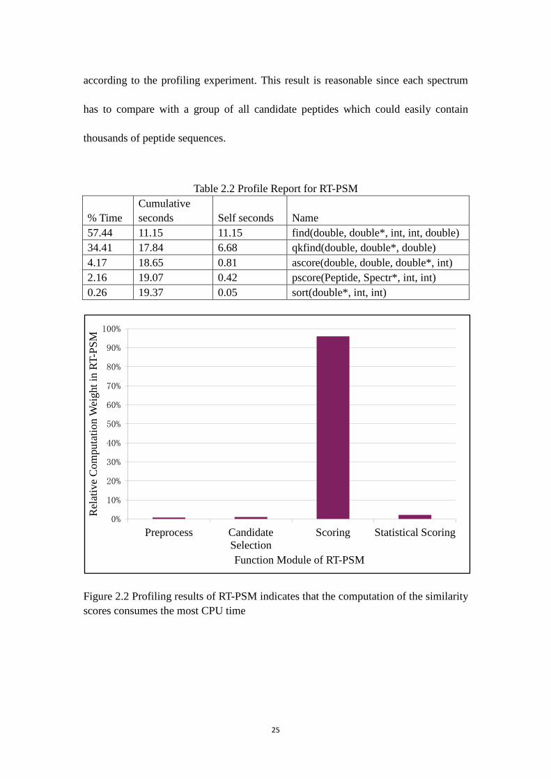
25
according to the profiling experiment. This result is reasonable since each spectrum
has to compare with a group of all candidate peptides which could easily contain
thousands of peptide sequences.
Table 2.2 Profile Report for RT-PSM
% Time Cumulative seconds Self seconds Name
57.44 11.15 11.15 find(double, double*, int, int, double) 34.41 17.84 6.68 qkfind(double, double*, double) 4.17 18.65 0.81 ascore(double, double, double*, int) 2.16 19.07 0.42 pscore(Peptide, Spectr*, int, int) 0.26 19.37 0.05 sort(double*, int, int)
Figure 2.2 Profiling results of RT-PSM indicates that the computation of the similarity scores consumes the most CPU time
0%
10%
20%
30%
40%
50%
60%
70%
80%
90%
100%
Preprocess Candidate Selection
Scoring Statistical Scoring
Rel
ativ
e C
ompu
tatio
n W
eigh
t in
RT-P
SM
Function Module of RT-PSM

26
CHAPTER 3
RT-PSM WITH PARALLEL PROGRAMMING
3.1 Overall of Parallel Computing Technology
Traditionally, computer software is designed for serial computation. A computer
program consists of a series of instructions to solve a problem. The CPU executes
them one by one and only one instruction can be executed at a time. Traditional serial
computing has its transmission speed limitations: the speed of serial computation is
dependent on the speed of data moving. Because of the limitation of hardware and
budget, sometimes serial computing cannot satisfy performance requirements.
Therefore, in order to save time and resources, solve larger problems, provide
concurrency or use non-local resources [23], the concept of parallel computing was
developed in early 60's by Gene Amdahl. Nowadays, according to the level of
hardware support for parallelism, parallel computing might be roughly classified
within following groups: multi-core computing, distributed computing, cluster
computing (symmetric multiprocessing computing), massive parallel processing, grid
computing, general-purpose computing on graphics processing units (GPGPU), vector
processors, etc. By the statistical result in 2011, about 40% of parallel computing
systems were used in academic and research settings, and the statistical trends

27
indicated that "parallelism is the future of computing"[24].
In this study, multi-core computing and cluster computation are used to create a new
algorithm to speed-up the RT-PSM procedure based on the existing laboratory
hardware. Based on Amdahl's law [25], the number of functions which could be
parallelized decides the speed-up of whole program. Hence, the speed of RT-PSM
could be rapidly progressed after it has been parallelized.
3.2 SIMD vs Multi-Core Computing
Multithreading technology has been implemented for decades. At least in 1992 when
Microsoft Foundation Class Library (MFC) was introduced with Microsoft's C/C++
7.0 compiler, it already contained the multithreading API to create and maintain
threads [26]. However, for most regular users, the early multithreading functions were
mostly used for data input/output or user interface (UI) design, not for computation
performance.
There are two types of computations classified by the hardware, CPU-bound
computation and I/O-bound computation. A CPU-bound computation is a computation
that spends most of its time keeping the CPU busy. I/O-bound computations are
computations that spend most of their time waiting for an I/O request to finish [27].
Reading files, downloading files or UI functions are typical I/O-bound computations.

28
In general, data transmission speed is far less than the CPU speed and that means that
the CPU spends most of its time on waiting for I/O requests. For CPU-bound
computation, CPU is always busy until the computation is over. Unless the computer
contains multiple CPUs, a CPU-bound computation cannot execute faster in multiple
threads than in a single thread. The reason is that for a single-core CPU, all
CPU-bound computations can only be executed in sequence. Before multi-core CPU
appeared, if a group of computations were executed in multiple threads, the
single-core CPU still can only execute them one by one and also needs time for
creating threads and switching the CPU between threads. The performance of
multithread CPU-bound computation could be slower than single thread one in a
single-core CPU. Therefore, multithreads cannot improve large scale computation
performance, such as matrix manipulations, operations on graphs with a single-core
CPU.
All this changed in 2002 when Intel introduced Hyper-Threading (HT) technology,
the first appearance of simultaneous multithreading technology in a consumer-grade
CPUs. With HT technology a physical CPU with single core can provide 2 logical
cores and execute two threads simultaneously. Then multithreading can be used in the
complex and/or large scale computations. Because with HT each logical core can
execute one CPU-bound computation concurrently, it can also be called multi-core
computing. In 2006, Intel released dual-core processer which was the first
consumer-grade CPU with multiple physical cores. Then the multi-core CPU became

29
the mainstream.
Single instruction multiple data (SIMD) is a type of parallel computing within all
processing units execute the same instruction at any given clock cycle and each
processing unit can operate on a different data element as shown in Figure 3.1 [23].
The SIMD technology was first used in 1970s. The first widely-deployed desktop
SIMD was Intel's Pentium MMX CPU. Actually, most CPU manufacturers, such as
HP, Sun, IBM or Sony all designed their own CPUs with SIMD technology. Although
all these SIMD technologies share common ideas and general operations, because of
differences in standards, the CPUs from different manufacturers have different
capabilities. For example, Sony's "Cell processor" can support from 8-bits to 128-bits
in size while Intel's AVX SIMD instructions now process 256 bits of data at once [15].
prev instruct prev instruct prev instruct time
load A(1) load A(2) load A(n)
load B(1) load B(2) load B(n)
C(1)=A(1)*B(1) C(2)=A(2)*B(2) … C(n)=A(n)*B(n)
store C(1) store C(2) store C(n)
next instruct next instruct next instruct
P1 P2 … Pn
Figure 3.1 SIMD: each processing can operate on a different data element with the same instruction at any given clock cycle
Before the HT technology was implemented in the consumer-grade CPUs, using

30
SIMD technology to implement parallelization for CPU-bound computation in
single-core CPUs was the mainstream. With SIMD at a given clock cycle, each
processing unit can execute the same instruction on different data. For the problems
that have a high degree of regularity, such as graphics or image processing, SIMD is a
good option for improving performance. It can also be used for complex computations,
such as data search or matrix manipulations. For the RT-PSM program, the peptide
database searching module and similarity scoring module can all be re-designed to
adapt SIMD to improve their performance [13, 28]. Without upgrading any hardware
to improve the computation performance, SIMD seems a suitable solution for this
study.
SIMD also has its disadvantages: lack of support in development environments,
unintended effects of changes in data precision and performance bottlenecks due to
cache misses. Most general software development kits include the multithreading
APIs. On the contrary, most SIMD APIs are directly facing to the registers and L2
cache, and can only work in C/C++ environments. Some of them even need use
assembly languages. All these restrictions make SIMD becoming a not
"developer-friendly" technology.
In order to achieve the best performance for Streaming SIMD Extensions (SSE) and
Streaming SIMD Extensions 2 (SSE2) instructions that operate on 128-bit registers,
data must be stored on 16-byte boundaries. Access to unaligned data with SSE

31
instructions is much slower than aligned access [29, 30]. The original RT-PSM
converts unaligned data to 32-bit single numbers. As a result, if each SSE register
(usually 128-bit) is divided into four 32-bit units, these 4 units can be operated upon
simultaneously. If the data precision of RT-PSM needs to be upgraded in the future,
using 64-bit double-precision number instead of 32-bit, each SSE register can only be
divided into 2 units. The computation performance will be reduced.
With SIMD technology, even though each processing unit can execute the same
instruction independently, the results are still stored in the same L2 cache. This means
that in a multi-core CPU, the size of L2 cache could become a bottleneck for SIMD
performance, to the point where the performance of a multithreading SIMD might not
be better than a single-core CPU. For example, consider a 2-core CPU with 1MB L2
cache and one single-core CPU also with 1MB L2 cache. They all have the same
128-bit SSE registers. In each core, each SSE register is divided into 4 32-bit units,
and each unit needs 250KB memory to store/transfer data. For the 2-core CPU, in
principle it should have a speed-up of 4*2 = 8 times. However, in the multithreading
model, the L2 cache does not have enough space to store the data from 2 threads
(250KB*4*2 = 2MB), which causes a higher rate of cache miss. On the other hand,
the L2 cache of the single-core CPU has enough space for the transmission data
(250KB*4 = 1MB), and the L2 cache miss rate is much lower. As a result, the SIMD
performance in the 2-Core CPU might be equal or even less than that in the
single-core CPU. So far, SIMD can achieve maximum performance for the original

32
RT-PSM program. Once the RT-PSM algorithm is updated and hits a specific memory
boundary, multithreading SIMD might not be able to satisfy the computation
requirements.
Generally speaking, in current circumstances, SIMD provides efficient parallel
computing performance, but it is more difficult to develop and maintain than
multi-core computing. The biggest disadvantage of SIMD is that its expandability is
quite limited. Therefore, in this study the parallel algorithm is based on the multi-core
computing technology on a multi-core CPU.
3.3 Database vs Datastore
Peptide database search is the first step of the similarity scoring module. There are
two factors affecting database search performance: the capabilities of the peptide
database and the similarity search algorithm. For the database, it is a dilemma whether
to choose a Structured Query Language (SQL) database or a data structure to store
data directly in memory. The most obvious choice is using the regular SQL database,
such as Oracle, Microsoft SQL server, MySQL, etc, since the SQL database is widely
used and has sufficient supports. In addition, it can be a supported by a separate
computation on its own thread(s). However, both database and datastore have their
cons and pros, and comparing them can help choose the most suitable one for this
study.

33
3.3.1 The advantages of SQL database
Queries: All SQL databases support standard SQL query language, and this makes
data search quite convenient. The SQL database is optimized for the search functions
and the user can also use "JOIN" to connect different tables to obtain complicated
information. The SQL language is easy-to-use and fully-functional. Given its high
level of abstraction, the user can pay more attention to how to create efficient query
statements instead of considering the performance of search algorithms or low-level
data structures. Another superiority of SQL is that if the peptide database needs to be
updated or moved to other SQL database in the future, the queries would be easy to
update and adapt the new database due to the SQL language standards.
Transactions: In order to support the multithread RT-PSM, the peptide database
should be able to support concurrent data transmission to reach the maximum
multithread RT-PSM performance. With correct configuration, the SQL database can
natively support concurrent transactions, while developers who use a datastore
approach have to design the concurrent connections and handle the data race directly.
Fortunately, in the original RT-PSM, the peptide database is only used to provide the
search results and does not need to consider the data race. If the peptide database
needs to expand the data store function in the future, it could be an issue which has to
be thought over.
Preload time: In most case, the SQL database should be active when the server is

34
turned on and the identification program should be able to access the database
anytime through database connections. On the other hand, a datastore needs to load
the data from storage files to main memory every time the program is executed.
Theoretically, for a 32-bit operating system, the maximum file load size is 4 GB and
the file size in 64-bit operating system is practically infinite. In practice, if the data
file is over 4 GB, the data preloading time is too long to affect the whole program
performance. When the file size is over the physical memory of the computer, the data
search performance could be dramatically decreased. That means the size of the data
files will affect the data preload time and the main memory of the computer will also
affect the inefficiency of the database loading into memory. All those factors could
lower program performance.
3.3.2 The shortages of SQL database
Management: To efficiently use a SQL database, the developer needs to have a certain
level of knowledge about database configuration, the SQL language and system
maintenance. If the data records or table structures need to be changed, the developer
cannot change them directly but has to use SQL languages. If a datastore is used on
the other hand, there is no configuration needed. Once the "table" needs to change, the
developer only needs to update the data structure. The data can also be changed by
directly changing the data store files.
Data transmission performance: In the cluster environment, the SQL database is

35
usually support by the head node where it is easy to manage for the developers.
Therefore, for each work node, the data has to transmit through the interconnection
fabric. Even if the cluster uses a low-latency/high-bandwidth network, the average
data transmission time from the head node's SQL database to a work node can be as
much as 0.3 second per task (based on local empirical tests). If a datastore is used,
because all data can be preloaded into each work node's memory, the data
transmission time is negligible.
Based on all these factors, the size of peptide database will decide which data store
methodology could provide best performance. The peptide database is derived from
the protein database and its size is about 4-6 times larger than the original protein
database. The complete UniRef100 protein database which is downloadable from
Universal Protein Resource is over 4 GB while the derived peptide database can
easily be over 10 GB. With this huge dataset, even though a computer can preload it
completely into its memory, the preloading time and peptide search time could be
unacceptable. In this case, using SQL database to manage the dataset and queries will
be the best choice. For those smaller peptide databases, if the user feels preloading
time does not affect the system performance, it may be better to use datastore because
the short data transmission time should be able to compensate for the performance
lost in the preload phase. In this study, both database and datastore interface are
provided to handle different needs. However, considering that the experiment dataset
is not very large (about 30 MB), all performance tests will be under datastore model.
36
3.4 Algorithm and Implementation
The original sequential RT-PSM program consists of four main functions which are
described previously. The similarity scoring function is a typical CPU-bound
computation function. That means the computing time of this function is dominated
by the speed of CPU. In order to achieve the best performance, one processor can
only execute one function at one time. The HT technology makes it possible to
execute multiple scoring functions concurrently in a single-CPU workstation [31].
That means the program can match multiple spectral groups simultaneously and
reduce the total execution time.
3.4.1 Parallel programming design pattern
In parallel programming, the main design principle is to balance the load among
multiple processors and to reduce communication overheads between processors.
Different design patterns can help developers to adapt different conditions, and
choosing the correct design pattern can reduce potential deficiencies [32, 33].
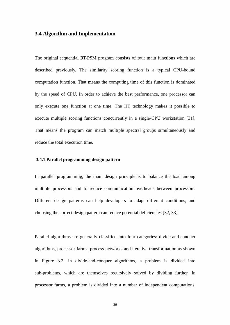
Parallel algorithms are generally classified into four categories: divide-and-conquer
algorithms, processor farms, process networks and iterative transformation as shown
in Figure 3.2. In divide-and-conquer algorithms, a problem is divided into
sub-problems, which are themselves recursively solved by dividing further. In
processor farms, a problem is divided into a number of independent computations,

37
and the results of these computations are combined by the controller. Process
networks are a division of computation with the data flowing through the stages. In
iterative transformation, sub tasks are transformed until the termination conditions are
satisfied through several iteration steps [33].
Figure 3.2 General classifications of parallel algorithms [33]
In this study, there are two different algorithms based on the underlying hardware

38
environments, a distributed computing algorithm and a multi-core algorithm. The two
algorithms use different design patterns. The distributed algorithm is used in a cluster.
The cluster consists of one head node and multiple work nodes. The head node
manages tasks and traces procedures. Hence, the hardware structure of a cluster is
suitable for the master/slave pattern. A processor farm is the most suitable design
pattern for the distributed computing algorithm.
On the other hand, for the multi-core algorithm each logical core is identical and
independent. There is no master/slave structure in the CPU structure. Secondly, in a
cluster, most computation tasks are distributed into work nodes and the head note is
only used for controlling the work nodes. However, for the multi-core CPU, all
logical cores should be assigned computation tasks in order to achieve the maximum
performance [34]. Hence, the design pattern of the multi-core algorithm is more like a
combination of processor farm and iterative transformation. With this design, the
control (master) thread is abandoned and every threads of the multi-core RT-PSM
(MT RT-PSM) program become a calculation thread. Each logical core of the CPU is
used in the calculation functions of RT-PSM and the program should be able to
employ all the usable system resources. Each subtask assigned to a thread should also
be independent. As trade-off, each thread should be designed to handle data input,
with the exception of control and data collection functions which are handled by the
control thread. The algorithm of each thread is more complicated.

39
3.4.2 Parallel function selection
The similarity score function consumes over 95% CPU time according to the profiling
analysis. The parallelization of the similarity score function should be the core feature
of the multi-core algorithm. The time-consuming nature of the similarity score
function is due to the binary search for each amino acid residue since the similarity
score function executes the binary searches sequentially. One possible design is to use
parallel ion searching in the similarity score function. However, a preliminary
experiment indicated that the ion search is very efficient and each search only takes
less than 0.01 milliseconds. Parallelization also needs to consider the time necessary
for the overheads of creating, invoking and disposing of threads. Because of the latter
overheads the parallel ion search function could spend more time than the sequential
version, even if different ion search threads could be executed simultaneously.
Amdahl's law [25] states that the overall speed-up of a parallelized program is:
1(1−𝑃)+𝑃𝑁
(3.1)
Assume that the running time of the old computation was 1, 𝑃 is the proportion of a
program that can be made parallel, 𝑁 is the number of processors. The speed-up of a
program using multiple processors in parallel computing is limited by the sequential
fraction of the program. That means if not only the similarity score function can be
parallelized, but also other modules, such as candidate peptide selection, statistical
significance computation, then the performance of the whole program could be

40
maximized. Based on this idea, each thread of the MT RT-PSM was designed to
perform the complete RT-PSM processing. With this design, the maximum speed-up
of the MT RT-PSM depends on the number of threads invoked by the program. The
maximum number of threads that can be used in the MT RT-PSM is based on the
number of logical processors.
3.4.3 Thread affinity
"White Paper - Processor Affinity" defines that thread affinity enables binding or
un-binding of a thread to a physical CPU or a range of CPUs, so that the thread will
run only on the CPU or range of CPUs. In order to achieve the maximum performance,
one objective is to make each CPU 100% utilized when the program is executing.
Each logical core should perform one thread simultaneously. That means the MT
RT-PSM program should be able to distribute one and only one thread to each logical
core. In a Windows system, there is a system diagnostics library that enables
developers to interact with user processes. Developers can force a thread to run in a
specific CPU core by using the ProcessThread class in the system diagnostics library
to manually distribute each thread of a program. In addition, the Windows scheduler
also has the ability to dynamically distribute threads to different CPU cores to balance
the system load.
In the ideal situation, all threads are expected to begin at the same time to minimize
the time differences between different threads. Hence, if the Windows scheduler

41
causes a long delay between threads, all threads should be manually distributed and
triggered. Ayucar’s research [35] indicates that the windows scheduler can provide
efficient thread distribution and management performance. All his experiments have
implied that the Windows scheduler beats a manual thread affinity setup almost in
every case. Based on this result, all threads are automatically distributed and managed
by the Windows scheduler in this study. The CPU usage results of MT RT-PSM also
display the same conclusion. All threads start simultaneously and the Windows
scheduler achieves maximum CPU performance. Results are shown in Figure 3.3.
Figure 3.3 Windows scheduler simultaneously starts 4 threads of MT RT-PSM in 4 cores
3.4.4 General code optimization
The original RT-PSM source code was designed several years ago with VC++ 6.0.
VC++6.0 has been retired and as the successor C# can provide a better object-oriented
development environment. So C# is chosen to develop MT RT-PSM and refactor the
original VC++ source code. Some functions in the original source code are obsoleted.
With the support of .net 4.0 framework, the corresponding functions can provide
better performance. Those old functions are replaced.
After analyzed the workflow of the original source code, there were some function

42
redundancies that can potentially increase the computational complexity. For these
functions, the subroutines are needed to redesign or make some rearrangements to
ensure the maximum performance.
3.4.5 Algorithm
The similarity scoring function is a typical CPU-bound function. In order to achieve
the best performance, one processor can only execute one function at one time. That
means with a multi-core CPU, the program can match multiple spectral groups
simultaneously and reduce the total execution time as shown in Figure 3.4. The
maximum number of threads that can be used in the MT RT-PSM is based on the
number of logical processors. The pseudo code of MT RT-PSM algorithm is shown in
Algorithm 2.
Algorithm 2: Multi-core RT-PSM
Class PeptideIdentification Collection PeptideDB; //peptide database Collection ExperimentPeptideData; //experiment data function PIF() PeptideDBLoading (DBfile, PeptideDB); //load peptide database ExperimentalPeptideDataLoading(DataFile, ExperimentPeptideData); //load experiment data MaxThreadNum ← Maximun number of CPU logical cores //obtain thread number InitMultiThreadCalc(MaxThreadNum, PeptideDB, ExperimentPeptideData); //initial each thread StartThreadList(MaxThreadNum, PeptideDB, ExperimentPeptideData); //run multithread RT-PSM End function function Pipid (PeptideDB,ExperimentPeptideData) //RT-PSM algorithm Tolerance← user-defined peptide search tolerance value;

43
Collection score; // similarity score list for each OnePeptideGroup in ExperimentPeptideData do filter (OnePeptideGroup,PeptideDB); candidatePeptideData ← qkfind(OnePeptideGroup, PeptideDB, tolerance); //2-demensinal peptide search for each candidatePeptide in candidatePeptideData do msct ← cscore(OnePeptideGroup,candidatePeptideData); //similarity scoring function score.Add(msct + 1); Init Matrix evalue; if pscore(evalue, score) is true postive then display result; //statistical significance function End function End Class Class MultiThreadCalc // Multithread control class void function InitMultiThreadCalc(Thread, PeptideDB, ExperimentPeptideData) //initial one thread for i← 0;i<Thread; i++ do InitOneThreadPip(PeptideDB, ExperimentPeptideData); End function void function StartThreadList(Thread,PeptideDB, ExperimentPeptideData) // execute one thread for i← 0;i<Thread; i++ do ThreadList[i].Pipid(PeptideDB, ExperimentPeptideData);; End function End Class
Figure 3.4 The flowchart illustrates the process of a multi-core computing algorithm

44
in MT RT-PSM

45
CHAPTER 4
RT-PSM WITH DISTRIBUTED PROGRAMMING
4.1 Introduction
4.1.1 Distributed computing and cluster
A cluster consists of a set of connected computers that work together, so they can be
viewed as a single system. The nodes (computers used as servers) of a cluster are
usually connected through a low-latency/high-bandwidth network, in most cases a
local area network. A cluster has times of computation ability compared to each
individual node. Hence, the main purpose of cluster is to provide performance
computation through distributed computing algorithm.
The earliest cluster prototype appeared in 1960s and it mainly used to backup data.
Ten years after Gene Amdahl published his famous paper on parallel processing:
Amdahl's Law [25]. The first commercial clustering product was developed in 1977.
Nowadays, although the CPU frequency and the node number of a cluster have been
rapidly improved, the factors which affect the cluster performance never change:
processor performance, network, software infrastructure and development tools.
Early cluster system was more or less restricted by early networks since one of the

46
primary motivations for the development of a network was to link computing
resources. Modern cluster is more related on the CPU frequency and core numbers at
the hardware layer. The computational capability of modern clusters is far more better
the first generation ones.
The cluster software infrastructure develops more slowly than the hardware. Parallel
systems are useless without parallel software. Different with sequential program, the
control algorithm of parallel programming is much more complicated. So it is
impossible to generate parallel software automatically. In 1990s, there were still
dozens of parallel programming languages and most of them did not have a general
standard. In 1995 the Message Passing Interface (MPI) became the first development
standards [36] and it makes the parallel programming development easier than before.
An ideal cluster application development environment should include a stable
operation system and a set of development tools which can support the standard
parallel algorithm and libraries. The development environment for clusters must be
able to provide the tools that are currently available on cluster systems. The parallel
applications should be developed, debugged and tested on the cluster environment
through the development tools.

47
4.1.2 WINDOWS HPC library
The main cluster operating systems are either UNIX/Linux or windows. Not like
UNIX, Microsoft began to design their cluster OS after mid-90s based on Windows
NT Server 4.0 Enterprise Edition. In June 2006, Microsoft released Windows
Compute Cluster Server 2003 which was the first high-performance computing (HPC)
cluster technology offered by Microsoft. It also released the Windows HPC Server
2008 as the successor product. Windows HPC Server 2008 includes features unique to
HPC workloads: a new high-speed Network Direct RDMA, highly efficient and
scalable cluster management tools, a service-oriented architecture (SOA) job
scheduler, an MPI library based on open-source MPICH2, and cluster interoperability
through standards such as the High Performance Computing Basic Profile (HPCBP)
specification produced by the Open Grid Forum (OGF) [37].
Microsoft also provides cluster HPC SDK to help development cluster applications.
Compute Cluster Pack (CCP) has secure, scalable cluster resource management, a job
scheduler, and a MPI stack for parallel programming. Compared with Unix/Linux
system, Microsoft’s HPC Server + CCP + Visual Studio constitute an integrated,
efficient and user-friendly development environment.
With the definition of computer cluster for windows HPC system, it is a top-level
organizational unit. Each cluster consists of a set of nodes, queues, applications, and
jobs. The following Figure 4.1 shows the compute cluster architecture.

48
Figure 4.1 The flowchart illustrates Microsoft compute cluster architecture [37]
A node is a single computer that contains one or multiple CPUs. A cluster consists of
one head node and multiple work nodes. The head node manages the cluster resources
and distributes all jobs to work nodes. All nodes in a cluster are parts of the same
domain. Data sources, such as database or datastore systems are accessible from each
node. A cluster application can enumerate, approve, pause and resume nodes through
the ICluster interface. It is also able to query node properties through the INode
interface. There is an organizational unit in the cluster - job queue, which contains
queued, running and finished jobs.
The job scheduler service is the core scheduling service of the CCP. It controls
resource allocation, job execution and recovery on failure. It also manages the job
queue and removes the finished jobs periodically. The architecture is shown as the

49
following Figure 4.2.
Figure 4.2 The flowchart illustrates the job scheduler architecture [37]
As the core scheduling service, the job scheduler allocates the cluster resources by job
priority. This makes the high-priority jobs at the front of the queue. If jobs have
identical priority, resources are allocated to the job based on the first in first out (FIFO)
policy. There is no task priority within a job. All tasks are allocated in the order that
they are added to the job. The job scheduler selects the best available node to run each
job and the system administrator can also specify a list of nodes to run certain jobs.
The job scheduler supports backfill. This ensures a resource-intensive application will
not delay other applications when they are ready to run. If a high-priority job is
waiting for available resources, the job scheduler will execute the lower-priority job
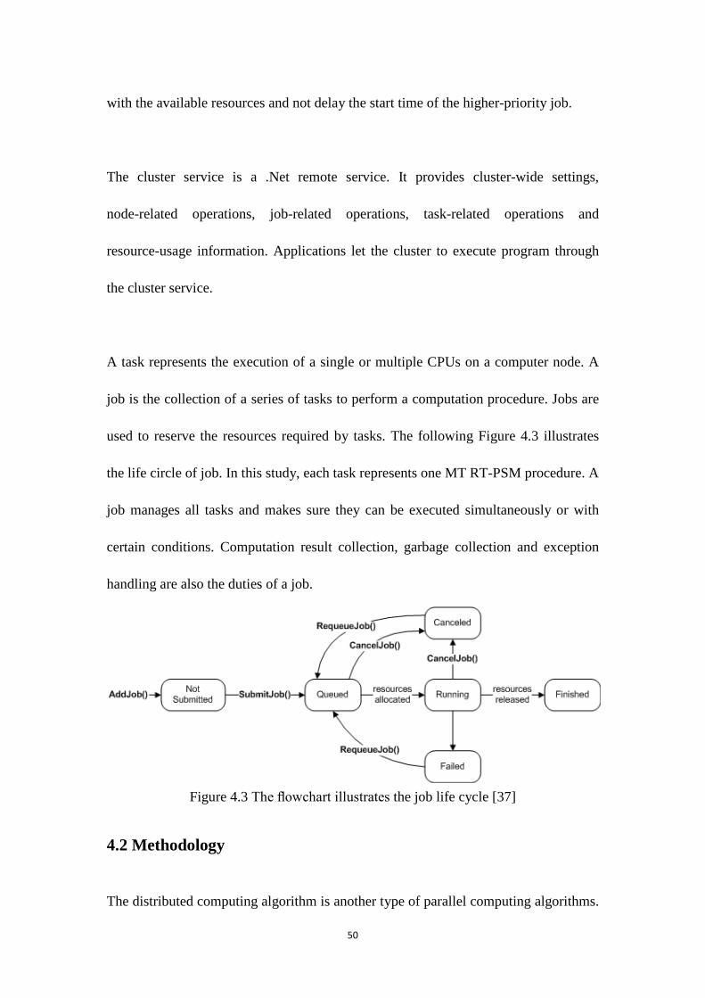
50
with the available resources and not delay the start time of the higher-priority job.
The cluster service is a .Net remote service. It provides cluster-wide settings,
node-related operations, job-related operations, task-related operations and
resource-usage information. Applications let the cluster to execute program through
the cluster service.
A task represents the execution of a single or multiple CPUs on a computer node. A
job is the collection of a series of tasks to perform a computation procedure. Jobs are
used to reserve the resources required by tasks. The following Figure 4.3 illustrates
the life circle of job. In this study, each task represents one MT RT-PSM procedure. A
job manages all tasks and makes sure they can be executed simultaneously or with
certain conditions. Computation result collection, garbage collection and exception
handling are also the duties of a job.
Figure 4.3 The flowchart illustrates the job life cycle [37]
4.2 Methodology
The distributed computing algorithm is another type of parallel computing algorithms.

51
Similar to multi-core computing, it separates a large task into several sub-tasks and
executes them concurrently. The most critical difference between multi-core
computing and distributed computing is that in multi-core computing all processors
may access to a shared memory while in distributed computing each processor has its
own memory [35]. In this study, the whole identification procedure is divided into
several sub RT-PSM tasks. Then each sub-task runs in an individual node workstation
of the cluster. The head node's duty includes task creation, management and
synchronization instead of executing RT-PSM program. Those duties make the head
node a task controller.
In order to achieve the minimum execution time of the RT-PSM program, the head
node should have an algorithm to create, distribute, synchronize and monitor the tasks
of work nodes. The pseudo code of the distributed computing algorithm is shown in
Algorithm 3. This distributed computing RT-PSM (DC RT-PSM) algorithm contains
three main modules. The first module loads an experimental tandem mass spectra data
file and divides it into a user-defined number of small files. Then it points each small
file to a related work node. The second module creates the sub RT-PSM task in each
work node. Then it starts all tasks simultaneously. The third module monitors all tasks'
executions and collects the feedback information which includes the task status and
exceptions. After all tasks are accomplished, the DC RT-PSM collects the result of
work nodes and generates the final report. The Figure 4.4 shows the work flow of the
algorithm 3.

52
Algorithm 3 Distributed computing RT-PSM Class DCRTPSM int MaxNodeNum ←user-defined maximum number of work nodes; function CreateHPCJob ICluster cluster ← new Cluster; cluster.connect(); aJob ← cluster.CreateJob; for i← 0; i< MaxNodeNum; i++ do aTask ← cluster.CreateTask; // Create a new task set aTask.commandline; set aTask.Stdout; set aTask.Stderr; set aTask.RequirtNodes; set aTask.MaximumNumberOfProcessors; aJob.AddTask(aTask); End function function TrackHPCJob(jobID) while aJob is not finished do aJob ← cluster.GetJob(JobID); check aJob status; handle aJob exceptions; End function //track node execution status function HPCJobResultCollection() //Collecting results from node i End Class

53
Figure 4.4 The flowchart illustrates the process of a distributed computing algorithm in DC RT-PSM
The time consumption of similarity scoring function in DC RT-PSM is:
𝑇𝑖 = 𝑀𝑎𝑥(𝐵𝑖 + 𝑆𝑖 + 𝐶𝑇𝑖) (4.1)
where 𝐶𝑇𝑖 is the message communication time and 𝑖 represents the number of
threads. The time consumption of message communication in each thread is fixed, so
when the program processes a large dataset, the database search time 𝐵𝑖 and scoring
time 𝑆𝑖 will be larger than a small dataset and the 𝐶𝑇𝑖 will less affect the total time
Ti than a small dataset. The total time consumption of the DC RT-PSM is:
𝑇𝑇𝑜𝑡𝑎𝑙 = 𝑇𝐼𝑛 + 𝑀𝑎𝑥(𝑇𝑛) + 𝑀𝑎𝑥(𝐶𝑁𝑇𝑛) (4.2)
where 𝑇𝐼𝑛 is the task initial time. 𝐶𝑁𝑇𝑛 is the node message communication time
and n is the number of nodes.

54
CHAPTER 5
MULTIDIMENSIONAL SEARCH: SPEED-UP PEPTIDE
DATABASE SEARCHING
In the similarity scoring module, the first step is to search the peptide database which
is derived from the protein database to obtain a suitable peptide as the start point of
the similarity scoring. The mass of match peptide Mm should be in the range of target
peptide mass Mt with a tolerance ε (𝑀𝑚 < 𝑀𝑡 ± 𝜀). That means the peptide database
search is a nearest neighbor search (NNS) [38, 39], also known as similarity search
instead of a regular search. The NNS describes the need to find the point among a
group of known positions which is closest to some randomly chosen probe position.
The original RT-PSM program uses a common linear search algorithm - binary search
to compute the distance from the query point to every point in database to obtain the
shortest distance. The time complexity of binary search equals to 𝑂(𝑙𝑜𝑔 𝑛), which is
related to the size of peptide database.
The regular database might contain random data, while the peptide database contains
the mass value of each peptide which is related to the peptide’s length and structure.
Two peptide sequences may have close mass values if their structures are similar. Two
different peptide sequences also can have the same mass value. From the
mathematical perspective, the peptide database can be viewed as a group of
consequent positive numbers.

55
Space partitioning which is an advanced NNS method might be able to take advantage
of this characteristic of peptide database. With this method the whole peptide database
can be divided into a series of small peptide groups (subsets) based on the candidate
peptide tolerance value instead of treading the whole peptide database as a large array
[40]. Each subset is indexed with the integer part of minor mass value and the integral
peptide database is a sorted collection that contains indexed sub-databases as shown
in Figure 5.1.
Original Peptide Database: ... 1811.0013 1811.0031 1811.0053 .. 1813.0333 1813.0421 1813.0466 ... 2-Dimentional Peptide Database:
Figure 5.1 2-Dimensional peptide database structures in contrast of original peptide database structures
With this new 2- dimensional peptide database, the peptide searching consists of two
parts. The first step is to search if the integer part 𝑋 of the target peptide mass with
tolerance value 𝑇 is indexed by the peptide database (𝑋 ± 𝑇). If the value is found,
then the first record in the indexed sub-array is the match peptide. The time
complexity of this step is 𝑂(2𝑇). If the first step cannot find a match peptide and the
database also contains a subset with index (𝑋 − 1), then the second step is to use the
X
Index Sub-array ... 1811 1811.00134 1811.00313 1811.00537 1811.00584 1811.00715 .... 1812 1812.0033 1812.01587 1812.01814 1812.02174 1812.02443 .... 1813 1813.00374 1813.02552 1813.03091 1813.03339 1813.04665 .... ...
Y

56
binary search method to find whether this subset contains match peptide. The time
complexity of the second step is 𝑂(𝑙𝑜𝑔(𝑠𝑢𝑏𝑠𝑒𝑡 𝑙𝑒𝑛𝑔𝑡ℎ)). The time complexity of
2-dimensinal peptide database search algorithm is much less than the original binary
search. The pseudo code of the algorithm is shown in Algorithm 4.
Algorithm 4 2-Dimensional Peptide Database Search function integer qkfind(OnePeptideGroup, PeptideDB, tolerance) //Multidimensional Search: if OnePeptideGroup.mass > PeptideDB.lastRecord.Mass OR OnePeptideGroup.mass < PeptideDB.firstRecord.Mass then return -1; else lowBoundary ← (OnePeptideGroup.mass - tolerance) + 1 ; upBoundary ← (OnePeptideGroup.mass + tolerance); for i ← lowBoundary; i< upBoundary; i++ do if PeptideDB hasIndex (i) then subSet ← PeptideDB.item(i); return subSet.firstItem.Index; else if PeptideDB hasIndex(lowBounday -1) then subSet ← PeptideDB.item(lowBounday -1); Index ← BinarySearch(subSet, OnePeptideGroup.mass) Return Index; End function
One advantage of 2-dimensional search is that its search speed is not directly
depending on the size of database but the density of indexed subsets in certain range.
The higher density brings higher hit-rate which helps to improve the speed of entire
peptide identification procedure. Another advantage is that this search algorithm does
not need supports from any third party databases. Compared with other parallelized
database search algorithms, this algorithm only need slightly change the peptide
database structures.
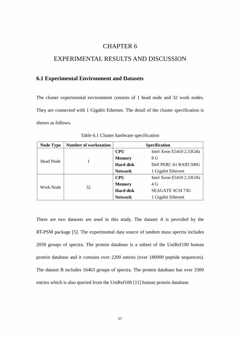
57
CHAPTER 6
EXPERIMENTAL RESULTS AND DISCUSSION
6.1 Experimental Environment and Datasets
The cluster experimental environment consists of 1 head node and 32 work nodes.
They are connected with 1 Gigabit Ethernet. The detail of the cluster specification is
shown as follows.
Table 6.1 Cluster hardware specification
Node Type Number of workstation Specification
Head Node 1
CPU Intel Xeon E5410 2.33GHz Memory 8 G Hard disk Dell PERC 6/i RAID 500G Network 1 Gigabit Ethernet
Work Node 32
CPU Intel Xeon E5410 2.33GHz Memory 4 G Hard disk SEAGATE SCSI 73G Network 1 Gigabit Ethernet
There are two datasets are used in this study. The dataset A is provided by the
RT-PSM package [5]. The experimental data source of tandem mass spectra includes
2058 groups of spectra. The protein database is a subset of the UniRef100 human
protein database and it contains over 2200 entries (over 180000 peptide sequences).
The dataset B includes 16463 groups of spectra. The protein database has over 3300
entries which is also queried from the UniRef100 [11] human protein database.

58
6.2 Verification
The verification of RT-PSM results is an essential part of this study. The purpose of
parallel computing algorithm is not only to reduce the peptide identification procedure
execution time, but also to keep the identification accuracy at the same time. The MT
RT-PSM does not use any trade off algorithm to gain better performance. Therefore,
the results of MT RT-PSM should be identical with the original RT-PSM. 10 groups of
experimental data are randomly chosen from the results of MT RT-PSM and original
RT-PSM. They are shown in the Table 6.2. Overall, the identification results are in
excellent agreement between MT RT-PSM and original RT-PSM.
Table 6.2 Result comparison between MT RT-PSM and original RT-PSM 5 columns to compare, the charge of spectrum, the similarity score and the match (-1 for not match, 1 for match)
Multithread Spec Index Spec Sequence Charge msc match
141 TQETPSAQMEGFLNR 2 1.63 -1 256 DVSGPMPDSYSPR 2 2.41 -1 489 NLLHVTDTGVGMTR 3 1.29 -1 812 NALESYAFNMK 2 1.35 -1 904 ALEQFATVVEAK 2 1.52 -1 1010 AIADTGANVVVTGGK 2 1.91 -1 1149 ILLAELEQLK 2 1.61 -1 1551 SSGSPYGGGYGSGGGSGGYGSR 2 1.41 1 1619 CATSKPAFFAEK 3 2.05 1 1755 YLAEFATGNDR 2 2.16 1
Original Spec Index Spec Sequence Charge msc match
141 TQETPSAQMEGFLNR 2 1.63 -1 256 DVSGPMPDSYSPR 2 2.41 -1 489 NLLHVTDTGVGMTR 3 1.29 -1 812 NALESYAFNMK 2 1.35 -1 904 ALEQFATVVEAK 2 1.52 -1

59
1010 AIADTGANVVVTGGK 2 1.91 -1 1149 ILLAELEQLK 2 1.61 -1 1551 SSGSPYGGGYGSGGGSGGYGSR 2 1.41 1 1619 CATSKPAFFAEK 3 2.05 1 1755 YLAEFATGNDR 2 2.16 1
6.3 Peptide Database Search Speed-up
Using experimental dataset A as an example, comparing similarity scoring time by
using linear search method and 2-dimensional search method, the new search
method makes similarity scoring module spent less than 6.7% execution time as
shown in the Table 6.3.
Table 6.3 Result comparison between linear search and 2-demensional search
Groups of Spectra Average Similarity scoring time (ms)
linear search 2058 8.043
2-dimensional search 2058 7.668
This 2-dimensional search algorithm cannot improve the accuracy of candidate
peptide selection, but it can speed-up the procedure to a certain degree. RT-PSM is a
complicated computation system and there is no simple solution to speed-up the
whole system with one upgrade. The improvement of whole system must be
contributed by the improvement of each sub-system. Although, the 2-dimensional
search algorithm only brings less than 7% improvement, it might be able to inspire the
future developers to design a better algorithm to rapidly speed-up the NNS without

60
any accuracy trade-off.
6.4 Multithread RT-PSM Performance
The performance of multithread RT-PSM mainly depends on the speed of CPU
frequency and the maximum number of logical cores of CPU. MT RT-PSM is tested
in 4 different computers and the Table 6.4 displays the detail information of the CPUs.
Table 6.4 Experiment hardware environment information
Name CPU # of Physical Cores HT Usage WS1 I7 3770 4 YES Personal server WS2 I5 750 4 NO Development PC WS3 XEON E5410 8 NO Work node of Cluster WS4 I7 2720QM 4 YES Personal computer
Figure 6.1 Speed-up of execution time for MT RT-PSM benchmark to original RT-PSM in 4 experiment computers
Figure 6.1 displays the speed-up between original RT-PSM program and MT RT-PSM
1
6
11
16
21
26
31
36
1 2 3 4 5 6 7 8
Spee
dup
Thread Number
Original RT-PSM vs MT RT-PSM
WS1
WS2
WS3
WS4

61
program with the same experiment dataset (dataset A). The result indicates several
improvements of MT RT-PSM compared with original program. Firstly, the
performance has been already progressed with refactoring and using .net framework
to optimize the original program. Even only using single-thread, the MT RT-PSM
achieves about 5 times speed-up than original RT-PSM program. Secondly, the
program execution time is continuously decreased when more threads are involved.
This result confirms the Amdahl's law that the program execution time should
decrease when the thread number increases. The last, for those CPUs which have 8
logical cores, the MT RT-PSM can achieve about 25 to 34 times speed-up when all
available cores were involved in the computing. The speed of peptide identification
procedure is promising.
Figure 6.2 displays the speed-up of MT RT-PSM program executing with multiple
threads against single-thread in 4 experiment computers. The result illustrates that the
disagreement between the theoretical speed-up and the practical performance
improvement can be massive due to different experimental environment. The
computer WS3 is one work node of the cluster. It represents the most stable
performance and reaches best speed-up when its maximum logical cores are assigned
in computing. On the contrary, WS1 and WS4 are regular standalone computers
which are mostly using for daily duties and application development. They need
spend a certain amount of resources to maintain the routine tasks. It is very difficult to
let a standalone workstation invoke all system resources to process the MT RT-PSM.

62
Figure 6.2 Speed-up of execution time for MT RT-PSM benchmark to single thread MT RT-PSM in 4 experiment computers
Generally speaking, the CPU frequency and the number of logical core are the most
important part of the performance. Nevertheless, the MT RT-PSM can only reach the
best performance when the system distributes the maximum resource into the
computation.
6.5 Distributed Computing RT-PSM (DC RT-PSM) Performance
The similarity scoring of single-thread RT-PSM search of 2058 group spectra against
2200-entry protein database (experiment dataset A) spent about 53, 105 and 125 times
1
2
3
4
5
6
7
8
1 2 3 4 5 6 7 8
Spee
dup
Thread Number
MT RT-PSM: Single thread vs multiple thread
WS1
WS2
WS3
WS4

63
than the similarity scoring of DC RT-PSM search in the same condition when it was
allocated into 80 threads (10 work nodes), 160 threads (20 work nodes) and 240
threads (30 nodes), respectively. The similarity scoring of single-thread RT-PSM
search of 16463 group spectra against 3200-entry protein database (experiment
dataset B) spent about 69, 155 and 127 times than the scoring of DC RT-PSM when
the task was allocated into 80, 160 and 240 threads. Figure 6.3 illustrates the
comparison results.
Figure 6.3 Speed-up of similarity scoring module execution time for DC RT-PSM benchmark to single thread MT RT-PSM from experiment dataset A (blue line) and experiment dataset B (red line)
No matter 80, 160 or 240 threads are allocated; the whole DC RT-PSM search is about
1.00
53.64
105.11
124.91
1.00
69.09
155.37
216.90
0
50
100
150
200
250
0 50 100 150 200 250
Spee
dup
Thread Number
Similarity Scoring Module Speedup
Experiment Dataset A Experiment Dataset B

64
11 times faster than the single-thread MT RT-PSM search with experiment dataset A.
With experiment dataset B, DC RT-PSM search execution time is 48 times speed-up
with 80 threads, 68 times speed-up with 160 threads and 85 times speed-up with 240
threads compared to single-thread MT RT-PSM search. This is shown in Figure 6.4.
Overall, the time benchmarks indicate a great performance upgraded by DC RT-PSM.
Figure 6.4 Speed-up of execution time for DC RT-PSM benchmark to single thread MT RT-PSM from experiment dataset A (blue line) and experiment dataset B (red line)
With 30 nodes and each nodes contains 8 logical processors, the DC RT-PSM
program should be able to gain 240-fold speed-up. Compared with experiment dataset
A and B in Figure 6.3, the performance is close to the theoretical performance when
DC RT-PSM processes large spectrum dataset against large database.
1.00 11.05 11.05 11.05
1.00
48.44
67.82
84.78
0
50
100
150
200
250
0 50 100 150 200 250
Spee
dup
Thread Number
DC RT-PSM Speedup
Experiment Dataset A Experiment Dataset B
65
In DC RT-PSM, the task initializing time and node message communication time are
fixed. Even the nodes are connected with 1 gigabit Ethernet, the time lost in those
processes are about 2.0 to 2.3 seconds. Therefore, if the experimental spectrum
dataset is too small, the number of nodes allocated in the task can barely affect the
total execution time, just like it shows experiment dataset A in Figure 6.4.
Compared Figure 6.3 to Figure 6.2 of MT RT-PSM, the performance of DC RT-PSM
is closer to the theoretical maximum value. The reason is that in the cluster, the
computation is preformed in the work nodes that are more focus on computational
tasks than other services. Therefore, the cluster is a more stable platform to process
large scale computational tasks than standalone workstations.
Generally, the performance of DC RT-PSM is related to the number of processors
allocated in the task and the size of experimental dataset. For small datasets, if the
total similarity scoring time is less than certain number, it is 500 milliseconds for this
study, adding more nodes in the task may not be able to reduce the total execution
time.
6.6 Discussions
In “Parallel Tandem”, Duncan et al. [12] developed a cluster system and achieved
18-fold faster with 20 processors and 36-fold faster with 40 processors for unrefined
searches. The speed-up for refined searches is about 10-fold with 40 processors.

66
Zhang et al.’s study [13] also uses Prof. Wu’s RT-PSM algorithm and consists with
two parts: SIMD in single CPU and CUDA in NVIDIA GPU. Their study achieves
about 18-fold speed-up for single CPU version. In CUDA version, a 190-fold
speed-up on the scoring module is achieved and 26-fold speed-up on the entire
process is obtained.
In this study, the MT RT-PSM achieves 25 to 34 folds speed-up for the entire process
with different single-CPU computers. The DC RT-PSM achieves about 217-fold with
240 processers for the similarity scoring and about 85-fold for the entire process. This
result shows that DC RT-PSM is about 90% scalable for the parallel portion of the
similarity scoring. The high percentage of scalable implies the better performance
with parallel computing. This value is similar with Duncan et al.’s speed-up of
parallel unrefined searches and better than their refined searches. The performance of
MT RT-PSM and DC RT-PSM are better than Zhang et al.’s SIMD version and CUDA
version programs. Generally, the performance improvements of this study are better
than the study of Duncan et al. and Zhang et al.

67
CHAPTER 7
CONCLUSIONS AND FUTURE WORK
7.1 Conclusions
In this study, a DC RT-PSM package is designed and consists of the multi-core
computing algorithm for standalone workstation and the distributed computing
algorithm for cluster. The multi-core computing algorithm is based on the original
single-thread RT-PSM. The distributed computing algorithm is used to allocate the
cluster nodes and manage the protein identification processing. This distributed
computing algorithm is designed not only for this RT-PSM algorithm but also for
other similar algorithms as a general parallel computing platform. It can support other
peptide identification programs with some configuration adjustments, such as
X!Tandem, CUDA version RT-PSM, etc.
The time required to match a large numbers of tandem mass spectra with peptides in a
database has been remarkably improved by performing searches concurrently with the
DC RT-PSM without sacrificing any matching accuracy. Overall, after upgraded with
the parallel computing algorithm, the DC RT-PSM program can achieve the
requirements of real-time peptide-spectrum matching processing. As a distributed
computing platform, the DC RT-PSM is a successfully implement in a highly
cost-effective parallel computing environment.

68
7.2 Future Work
There are still several parts of this study that could be improved in the future.
1. The distribution computing platform can only support the RT-PSM algorithm for
now. However, in the original design it should have the ability to handle different
programs and not just be limited to one particular peptide identification algorithm.
If there is any study related to large scale computation in cluster environment,
this platform could be a good start point.
2. In this algorithm, datastore is the main method to process the peptide database.
But in this study, the database connection interface is designed for both datastore
and database. Due to the time limitation, this study is not expended to use large
scale database in the RT-PSM algorithm. The optimization of large SQL database
also could be involved in the future work.
3. The DC RT-PSM has a graph user interface (GUI), but a crude one. A good GUI
can help user improve efficiency and reduce the erroneous operations. This gives
much room for design better GUI for the future.

69
REFERENCES [1] O. D. Sparkman, "Mass spectrometry desk reference", Global View Pub,
Pittsburgh, 2000. [2] K. Zaidi, "(GC05) General Chapters 05", USP29-NF24, pp. 2705, 2010. [3] A. P. Snyder, "Interpreting Protein Mass Spectra: A Comprehensive Resource",
Oxford University Press, Oxford, New York, 2000. [4] C. Dass, "Fundamentals of contemporary mass spectrometry", John Wiley & Sons,
2007. [5] F. X. Wu, P. Gagne, A. Droit, G. G. Poirier, "RT-PSM, a real-time program for
peptide-spectrum matching with statistical significance", Rapid Commum. Mass Spectrom, vol. 20, pp. 1199–1208, 2006.
[6] K. J. Eng, A. L. McCormack, J. R. Yates III, "An approach to correlate tandem
mass spectral data of peptides with amino acid sequences in a protein database", Am. Soc. Mass Spectrom, vol.5, pp. 976-989, 1994.
[7] D. N. Perkins, D. J. Pappin, D. M. Creasy, J. S. Cottrell, "Probability-Based
Protein Identification by Searching Sequence Databases Using Mass Spectrometry Data", Electrophoresis, vol.20, pp. 3551-3567, 1999.
[8] M. C. Damsten, J. N. M. Commandeur, A. Fidder, A. G. Hulst," Liquid
Chromatography/Tandem Mass Spectrometry Detection of Covalent Binding of Acetaminophen to Human Serum Albumin", Drug Metabolism and Disposition, vol. 35, No. 8, pp. 1408-1417, 2007.
[9] D. J. Rigden, "From Protein Structure to Function with Bioinformatics", Springer
Science, 2009. [10] B. Ma, R. Johnson, "De Novo Sequencing and Homology Searching", Mol Cell
Proteomics, vol.11, doi: 10.1074/mcp.O111.014902, 2012. [11] "Universal Protein Resource", http://www.uniprot.org. [12] D. T. Duncan, R. Craig, A. J. Link, "Parallel Tandem: a program for parallel
processing of tandem mass spectra using PVM or MPI and X!Tandem", Journal of Proteome Research, vol. 4, pp. 1842–1847, 2005.

70
[13] J. Zhang, I. McQuillan, F. X. Wu, "Parallelizing Peptide-Spectrum Scoring Using Modern Graphics Processing Units", IEEE ICCABS, vol.11, pp. 208-213, 2011.
[14] R. G. Sadygov, J. Eng, E. Durr, A. Saraf, H. McDonald, M. J. MacCoss, "Code
Developments to Improve the Efficiency of Automated MS/MS Spectra Interpretation", Journal of Proteome Research, vol.1, pp. 211–215, 2002.
[15] J. Zhang, I. McQuillan, F. X. Wu, "Speed Improvements of Peptide-Spectrum
Matching Using SIMD Instructions", Proteomics, vol. 11, Issue 19, pp. 3779–3785, 2011.
[16] G.S. Almasi, A. Gottlieb, "Highly Parallel Computing", Benjamin-Cummings
publishers, 1987. [17] A.Scherl, C. G. Zimmermann-Ivol, J. D. Dio," Gold coating of non-conductive
membranes before matrix-assisted laser desorption/ionization tandem mass spectrometric analysis prevents charging effect", Rapid Commum. Mass Spectrom, vol.19, pp. 605-615, 2005.
[18] B. Ma, "Challenges in computational analysis of mass spectrometry data for
proteomics", Science and Technology, vol.25, pp. 107-123, 2010. [19] S. Altschul, "The statistics of sequence similarity scores". NCBI: Cold Spring
Harbor, 2004, http://www.ncbi.nlm.nih.gov/BLAST/tutorial/Altschul-1.html. [20] H. I. Field, D. Fenyo, R. C. Beavis, "Radars, a bioinformatics solution that
automates proteome mass spectral analysis, optimizes protein identification, and archives data in a relational database", Proteomics, vol.2, pp. 36-47, 2002.
[21] D. Fenyo, R. C. Beavis, "A method for assessing the statistical significance of
mass spectrometry-based protein identifications using general scoring schemes", Anal. Chem, vol. 75, pp. 768-774, 2003.
[22] M. Havilio, Y. Haddad, Z. Smilansky, "Intensity-based statistical scorer for
tandem mass spectrometry", Anal. Chem, vol. 75, pp. 435-444, 2003. [23]B. Barney, "Introduction to Parallel Computing ", Lawrence Livermore National
Laboratory, 2012, https://computing.llnl.gov/tutorials/parallel_comp/. [24] A, Krste, "The Landscape of Parallel Computing Research: A View from
Berkeley", University of California, Berkeley, Technical Report No. UCB/EECS-2006-183, 2006.
71
[25] G. Amdahl, "Validity of the Single Processor Approach to Achieving Large-Scale Computing Capabilities", AFIPS Conference Proceedings, vol.30, pp.483–485, 1967.
[26] Blogs.msdn.com, "Quick Tour of New MFC functionality", 2007,
http://blogs.msdn.com/b/vcblog/archive/2007/11/09/quick-tour-of-new-mfc-functionality.aspx.
[27] R. R. Asche, "Multithreading Performance", 1996,
http://msdn.microsoft.com/en-us/library/ms810437.aspx. [28] T. Rognes, E. Seeberg, "Six-fold speed-up of Smith-Waterman sequence
database searches using parallel processing on common microprocessors", Bioinformatics, vol.16, pp. 699–706, 2000.
[29] F. Song, S. Moore, J. Dongarra, "L2 Cache Modeling for Scientific Applications
on Chip Multi-Processors", Parallel Processing, ICPP 2007, 2007. [30] D. Tarjan, J. Meng, K. Skadron, "Increasing Memory Miss Tolerance for SIMD
Cores", Proc. Supercomputing '09, 2009. [31] M. Ben-Ari, "Principles of Concurrent and Distributed Programming", Prentice
Hall, 1990. [32] S. Siu, M. D. Simone, D. Goswami, A. Singh, "Design Patterns for Parallel
Programming", in Proc. PDPTA, pp.230-240, 1996. [33] K. Yamazaki, S. Ando, "A Case-Based Parallel Programming System", PDSE '98,
pp. 238-246, 1998. [34] D. W. Holmes, J. R. Williams, P. Tilke, "An events based algorithm for
distributing concurrent tasks on multi-core architectures", Computer Physics Communications, vol. 181, pp. 341–354, 2010.
[35] I. Ayucar, "Parallel computing and processor affinity. Never underestimate the
Windows Vista Scheduler", 2009, http://www.codeproject.com/Articles/35679/Parallel-computing-and-processor-affinity-Never-un.
[36] D. A. Bader, R. Pennington, "Cluster Computing: Applications,'' The
International Journal of High Performance Computing, vol. 15(2), pp. 181-185, 2001.
[37] Microsoft, Microsoft HPC Pack 2008 SDK and HPC Pack 2008 R2 SDK, 2012,

72
http://msdn.microsoft.com/en-us/library/cc853440(v=vs.85). [38] S. Rajasekaran, J. Reif, "Handbook of Parallel Computing Models, Algorithms
and Applications", Chapman & Hall/CRC, 2007. [39] D. Dutta, T. Chen, "Speeding up tandem mass spectrometry database search:
metric embeddings and fast near neighbor search", Bioinformatics, vol.23, pp.612– 618, 2007.
[40] L. Andrews, "A template for the nearest neighbor problem", C/C++ Users Journal,
vol. 19, pp. 40 - 49, 2001.