parallel computation models - computer science | …vs3/comp422/lecture-notes/comp...parallel...

Vivek Sarkar

Department of Computer ScienceRice University

[email protected]

Parallel Computation Models

COMP 422 Lecture 20 25 March 2008

2 COMP 422, Spring 2008 (V.Sarkar)

Acknowledgements for today’s lecture

• Section 2.4.1 of textbook• Larry Carter, UCSD CSE 260 Topic 6 lecture: Models of

Parallel Computers– http://www-cse.ucsd.edu/users/carter/260/260class06.ppt

• Michael C. Scherger, “An Overview of the BSP Model ofParallel Computation”– http://www.cs.kent.edu/~jbaker/PDA-Sp07/slides/bsp%20model.ppt


Outline

• PRAM (Parallel Random Access Machine)• PMH (Parallel Memory Hierarchy)• BSP (Bulk Synchronous Parallel)• LogP


Review: The Random Access MachineModel for Sequential Computing

RAM model of serial computers:– Memory is a sequence of words, each capable of containing

an integer.– Each memory access takes one unit of time– Basic operations (add, multiply, compare) take one unit time.– Instructions are not modifiable– Read-only input tape, write-only output tape


PRAM [Parallel Random Access Machine]

PRAM composed of:– P processors, each with its own unmodifiable program.– A single shared memory composed of a sequence of words, each

capable of containing an arbitrary integer.– a read-only input tape.– a write-only output tape.

PRAM model is a synchronous, MIMD, shared address spaceparallel computer.– Processors share a common clock but may execute different

instructions in each cycle.

(Introduced by Fortune and Wyllie, 1978)


Architecture of anIdeal Parallel Computer

• Depending on how simultaneous memory accesses arehandled, PRAMs can be divided into four subclasses.– Exclusive-read, exclusive-write (EREW) PRAM.– Concurrent-read, exclusive-write (CREW) PRAM.– Exclusive-read, concurrent-write (ERCW) PRAM.– Concurrent-read, concurrent-write (CRCW) PRAM.


Architecture of anIdeal Parallel Computer

• What does concurrent write mean, anyway?– Common: write only if all values are identical.– Arbitrary: write the data from a randomly selected processor.– Priority: follow a predetermined priority order.– Sum: Write the sum of all data items.


Physical Complexity of anIdeal Parallel Computer

• Processors and memories are connected via switches.• Since these switches must operate in O(1) time at the

level of words, for a system of p processors and mwords, the switch complexity is O(mp).

• Clearly, for meaningful values of p and m, a true PRAMis not realizable.


More PRAM taxonomy

• Different protocols can be used for reading and writing sharedmemory.– EREW - exclusive read, exclusive write

A program isn’t allowed to have two processors access the samememory location at the same time.

– CREW - concurrent read, exclusive write– CRCW - concurrent read, concurrent write

Needs protocol for arbitrating write conflicts– CROW – concurrent read, owner write

Each memory location has an official “owner”• PRAM can emulate a message-passing machine by

partitioning memory into private memories.


Broadcasting on a PRAM

• “Broadcast” can be done on CREW PRAM in O(1) steps:– Broadcaster sends value to shared memory– Processors read from shared memory

• Requires lg(P) steps on EREW PRAM.

M

PPPPPPPP

B


Finding Max on a CRCW PRAM

• We can find the max of N distinct numbers x[1], ..., x[N] inconstant time using N2 procs!Number the processors Prs with r, s ε {1, ..., N}.– Initialization: P1s sets A[s] = 1.– Eliminate non-max’s: if x[r] < x[s], Prs sets A[r] = 0.

Requires concurrent reads & writes.– Find winner: If A[r] = 1, Pr1 sets max = x[r].


Some questions

1. What if the x[i]’s aren’t necessarily distinct?2. Can you sort N numbers in constant time?

And only use only Nk processors (for some k)?

3. How fast can you sort on CREW?4. Does any of this have any practical significance ????


PRAM is not a great success

• Many theoretical papers about fine-grained algorithmictechniques and distinctions between various modes.

• Results seem irrelevant.– Performance predictions are inaccurate.– Hasn’t lead to programming languages.– Hardware doesn’t have fine-grained synchronous steps.


Another look at the RAM model

• RAM analysis says matrix multiply is O(N3).for i = 1 to N for j = 1 to N for k = 1 to N C[i,j] += A[i,k]*B[k,j]

• Is it??


Matrix Multiply on RS/6000

T = N4.7

O(N3) performance would have constant cycles/flopPerformance looks much closer to O(N5)

Size 2000 took 5 days

12000 would take1095 years


Column major storage layout

cachelines

Blue row of matrix is stored in red cacheline


Memory Accesses in Matrix Multiply

for i = 1 to N for j = 1 to N for k = 1 to N C[i,j] += A[i,k]*B[k,j]

When cache (or TLB or memory) can’t hold entire B matrix, there will bea miss on every line.

When cache (or TLB or memory) can’t hold a row of A, there will be amiss on each access

Sequentialaccess throughentire matrix

Stride-Naccess toone row*

* assumes data is in column-major order


Matrix Multiply on RS/6000

Page miss every 512 iterations

Page miss every iteration

TLB miss every iteration

Cache miss every 16 iterations


Where are we?

• RAM model says naïve matrix multiply is O(N3)• Experiments show it’s O(N5)-ish• Explanation involves cache, TLB, and main memory

limits and block sizes• Conclusion: memory features are important and should

be included in model.


Models of memory behavior

Uniprocessor models looking at data access costs:Two-level models (main memory & cache):

Floyd (’72), Hong & Kung (’81)Hierarchical Memory Model

Accessing memory location i costs f(i)Aggarwal, Alpern, Chandra & Snir (’87)

Block Transfer ModelMoving block of length k at location i costs k+f(i)Aggarwal, Chandra & Snir (’87)

Memory Hierarchy ModelMultilevel memory, block moves, extends to parallelismAlpern & Carter (’90)


Memory Hierarchy model

A uniprocessor isSequence of memory modules

Highest level is large memory, low speedProcessor (level 0) is tiny memory, high speed

Connected by channelsAll channels can be active simultaneously

Data are moved in fixed-sized blocksA block is a chunk of contiguous dataBlock size depends on level

DISK

DRAM

cache

regs


Does MH model influence your thinking?

Say your computer is a sequence of modules:You want to move data to the fast one at bottom.Moving contiguous chunks of data is faster than moving inidividual

words

How do you accomplish this??One possible answer: divide & conquer


Visualizing Matrix Multiplication

C

B

A

“stick” of computationis dot product of a

row of A with column of B

cij= Σ aik∗ bkj

i

j C = A B


Visualizing Matrix Multiplication

C

B

A

“Cubelet” of computationis product of a submatrixof A with submatrix of B - Data involved is proportional to surface area. - Computation is proportional to volume.


MH algorithm for C = AB

Partition computation into “cubelets”Each cubelet requires sxs submatrix of A and B3 s2 data needed; allows s3 multiply-adds

Parent module gives child sequence of cubelets.Choose s to ensure all data fits into child’s memory

Child sub-partitions cubelet into still smaller pieces.Known as “blocking” or “tiling” long before MH model invented (but

rarely applied recursively).


Theory of MH algorithm for C = AB

“Uniform” Memory Hierarchy (UMH) model looks similar to actualcomputers.Block size, number of blocks per module, and transfer time per item grow

by constant factor per level.Naïve matrix multiplication is O(N5) on UMH.

Similar to observed performance.Tiled algorithm is O(N3) on UMH.

Tiled algorithm gets about 90% “peak performance” on many computers.Moral: good MH algorithm good in practice.


Visualizing computers in MH model

Height of module = lg(blocksize)Width = lg(number of blocks)Length of channel = lg(transfer time)

DISK

DRAM

cache

regs

This computer is reasonably well-balanced

This one isn’t

Doesn’t satisfy “widecache principle” (squaresubmatrices don’t fit).

Bandwidth too low


Parallel Memory Hierarchy (PMH) model

Alpern & Carter: “Since MH model is so great, let’s generalize it for parallelcomputers!”

A computer is a tree of memory modulesLargest memory is at root.Children have less memory, more compute power.

Four parameters per moduleBlock size, number of blocks, transfer time from parent, and number of

children.Homogeneous all modules at a level have same parameters

(PMH ignores difference between shared and distributed address spacecomputation.)

PMH ideas have influenced Sequoia language at Stanford


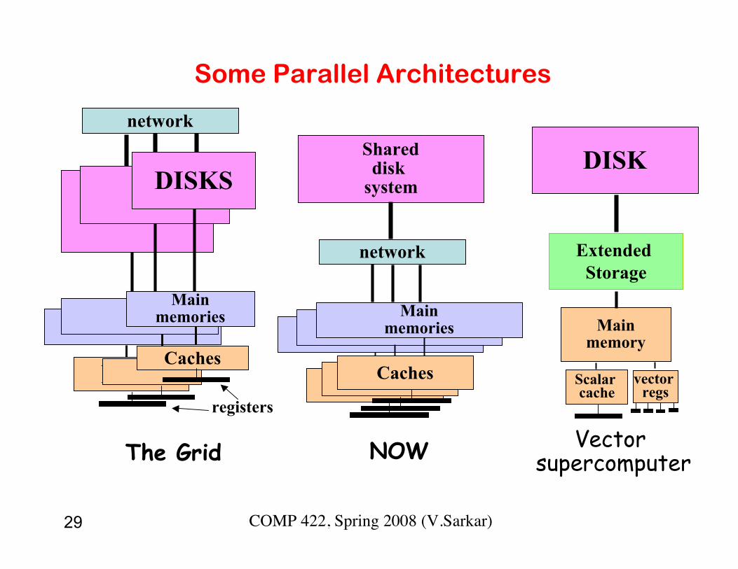
Some Parallel Architectures

The Grid

registers

Mainmemories

DisksCaches

network

NOW

DISKS

Mainmemories

Shareddisk

system

DisksDisksCaches

network

Mainmemory

DISK

Scalar cache

Extended Storage

vector regs

Vector supercomputer


PMH model of multi-tier computer

Secondary Storage

Internodal network

Node

L2

L1

P1

L2

L1

P2

Node

L2

L1

P3

L2

L1

P4

Node

L2

L1

...

L2

L1

Pn

functional units

DRAM

SRAM

MagneticStorage

registers


Observations

• PMH can model heterogeneous systems as well ashomogeneous ones.

• More expensive computers have more parallelism andhigher bandwidth near leaves

• Computers getting more levels & more branching.• Parallelizing code for PMH is very similar to tuning it for a

memory hierarchy.– Break computation into independent blocks– Send blocks of work to children

Needed for parallelization


BSP (Bulk Synchronous Parallel) Model

• Overview of the BSP Model

• Predictability of the BSP Model

• Comparison to Other Parallel Models

• BSPlib and Examples

• Comparison to Other Parallel Libraries


References

• “BSP: A New Industry Standard for Scalable Parallel Computing”,http://www.comlab.ox.ac.uk/oucl/users/bill.mccoll/oparl.html

• Hill, J. M. D., and W. F. McColl, “Questions and Answers About BSP”,http://www.comlab.ox.ac.uk/oucl/users/bill.mccoll/oparl.html

• Hill, J. M. D., et. al, “BSPlib: The BSP Programming Library”,http://www.comlab.ox.ac.uk/oucl/users/bill.mccoll/oparl.html

• McColl, W. F., “Bulk Synchronous Parallel Computing”, Abstract MachineModels for Highly Parallel Computers, John R. Davy and Peter M. Dew eds.,Oxford Science Publications, Oxford, Great Brittain, 1995, pp. 41-63.

• McColl, W. F., “Scalable Computing”,http://www.comlab.ox.ac.uk/oucl/users/bill.mccoll/oparl.html

• Valiant, Leslie G., “A Bridging Model for Parallel Computation”, Communicationsof the ACM, Aug., 1990, Vol. 33, No. 8, pp. 103-111

• The BSP Worldwide organization website is http://www.bsp-worldwide.org andan excellent Ohio Supercomputer Center tutorial is available at www.osc.org.


What Is Bulk Synchronous Parallelism?

• The model consists of:– A set of processor-memory pairs.– A communications network that delivers messages in a point-to-point

manner.– A mechanism for the efficient barrier synchronization for all or a subset

of the processes.– There are no special combining, replicating, or broadcasting facilities.

• In BSP, each processor has local memory. “One-sided” communicationstyle is advocated.– There are globally-known “symbolic addresses” (like VSM)

• Data may be inconsistent until next barrier synchronization• Valiant suggests hashing implementation of puts and gets.


BSP Programs

• BSP programs composed of supersteps.• In each superstep, processors execute up to L computational

steps using locally stored data, and also can send and receivemessages

• Processors synchronize at end of superstep (at which time allmessages have been received)

• Oxford BSP is a library of C routines for implementing BSPprograms. It provides:– Direct Remote Memory Access (a VSM layer)– Bulk Synchronous Message Passing (sort of like non-

blocking message passing in MPI)

superstep

synch

superstep

synch

superstep

synch


What does the BSP Programming StyleLook Like?

• Vertical Structure– Sequential composition of

“supersteps”.• Local computation• Process Communication• Barrier Synchronization

• Horizontal Structure– Concurrency among a fixed

number of virtual processors.– Processes do not have a

particular order.– Locality plays no role in the

placement of processes onprocessors.

– p = number of processors.

Virtual Processors

LocalComputation

GlobalCommunication

Barrier Synchronization


BSP Programming Style

• Properties:– Simple to write programs.– Independent of target architecture.– Performance of the model is predictable.

• Considers computation and communication at thelevel of the entire program and executing computerinstead of considering individual processes andindividual communications.

• Renounces locality as a performance optimization.– Good and bad– BSP may not be the best choice for which locality is critical


How Does Communication Work?

• BSP considers communication en masse.– Makes it possible to bound the time to deliver a whole set of

data by considering all the communication actions of asuperstep as a unit.

• If the maximum number of incoming or outgoing messages perprocessor is h, then such a communication pattern is called anh-relation.

• Parameter g measures the permeability of the network tocontinuous traffic addressed to uniformly random destinations.– Defined such that it takes time hg to deliver an h-relation.

• BSP does not distinguish between sending 1 message of lengthm, or m messages of length 1.– Cost is mgh


Barrier Synchronization

• “Often expensive and should be used as sparingly as possible.”

• Developers of BSP claim that barriers are not as expensive asthey are believed to be in high performance computing folklore.

• The cost of a barrier synchronization has two parts.– The cost caused by the variation in the completion time of

the computation steps that participate.– The cost of reaching a globally-consistent state in all

processors.

• Cost is captured by parameter l (“ell”) (parallel slackness).– lower bound on l is the diameter of the network.


Predictability of the BSP Model

• Characteristics:– p = number of processors– s = processor computation speed (flops/s) … used to calibrate g & l– l = synchronization periodicity; minimal number of time steps

between successive synchronization operations– g = total number of local operations performed by all processors in

one second / total number of words delivered by thecommunications network in one second

• Cost of a superstep (standard cost model):– MAX( wi ) + MAX( hi g ) + l ( or just w + hg + l )

• Cost of a superstep (overlapping cost model):– MAX( w, hg ) + l


Predictability of the BSP Model

• Strategies used in writing efficient BSP programs:– Balance the computation in each superstep between

processes.• “w” is a maximum of all computation times and the

barrier synchronization must wait for the slowestprocess.

– Balance the communication between processes.• “h” is a maximum of the fan-in and/or fan-out of data.

– Minimize the number of supersteps.• Determines the number of times the parallel slackness

appears in the final cost.


BSP Notes

• Number of processors in model can be greater than number ofprocessors of machine.Easier for computer to complete the remote memory operations

• Not all processors need to join barrier synch• Time for superstep = 1/s ×

(max (operations performed by any processor) + g × max (messages sent or received by a

processor, h0) + L)


Some representative BSP parameters

612800540,00061Pentium NOW

serial Ethernet 1

69540026IBMSP2

401.250647CrayT3E

32311830088Pentium II NOW

switched Ethernet

words (32b)n1/2 for h0

Flops/wordg

Flops/synchL

MFlop/ss

Machine(all have P=8)

From oldwww.comlab.ox.ac.uk/oucl/groups/bsp/index.html (1998)NOTE: Benchmarks for determining s were not tuned.


BSPlib• Supports a SPMD style of programming.

• Library is available in C and FORTRAN.

• Implementations available (several years ago) for:– Cray T3E– IBM SP2– SGI PowerChallenge– Convex Exemplar– Hitachi SR2001– Various Workstation Clusters

• Allows for direct remote memory access or message passing.

• Includes support for unbuffered messages for high performancecomputing.


BSPlib• Initialization Functions

– bsp_init()

• Simulate dynamicprocesses

– bsp_begin()

• Start of SPMD code– bsp_end()

• End of SPMD code

• Enquiry Functions– bsp_pid()

• find my process id– bsp_nprocs()

• number of processes– bsp_time()

• local time

• Synchronization Functions– bsp_sync()

• barrier synchronization

• DRMA Functions– bsp_pushregister()

• make region globallyvisible

– bsp_popregister()

• remove global visibility– bsp_put()

• push to remote memory– bsp_get()

• pull from remotememory


BSPlib

• BSMP Functions– bsp_set_tag_size()

• choose tag size– bsp_send()

• send to remote queue– bsp_get_tag()

• match tag with message– bsp_move()

• fetch from queue

• Halt Functions– bsp_abort()

• one process halts all

• High Performance Functions– bsp_hpput()

– bsp_hpget()– bsp_hpmove()

– These are unbuffered versionsof communication primitives


BSPlib Examples

• Static Hello World

void main( void ){ bsp_begin( bsp_nprocs());

printf( “Hello BSP from %d of %d\n”, bsp_pid(), bsp_nprocs());

bsp_end();}

• Dynamic Hello World

int nprocs; /* global variable */void spmd_part( void ){ bsp_begin( nprocs ); printf( “Hello BSP from %d of %d\n”, bsp_pid(), bsp_nprocs());}void main( void ){ bsp_init( spmd_part, argc, argv ); nprocs = ReadInteger(); spmd_part();}


BSPlib Examples

• Serialize Printing of Hello World (shows synchronization)

void main( void ){ int ii; bsp_begin( bsp_nprocs()); for( ii=0; ii<bsp_nprocs(); ii++ ) { if( bsp_pid() == ii ) printf( “Hello BSP from %d of %d\n”, bsp_pid(), bsp_nprocs()); fflush( stdout ); bsp_sync(); } bsp_end();}


BSPlib Examples

• All sums version 1 ( lg( p ) supersteps )int bsp_allsums1( int x ){

int ii, left, right;bsp_pushregister( &left, sizeof( int ));bsp_sync();right = x;for( ii=1; ii<bsp_nprocs(); ii*=2 ){

if( bsp_pid()+I < bsp_nprocs())bsp_put( bsp_pid()+I, &right, &left, 0, sizeof( int ));

bsp_sync();if( bsp_pid() >= I )

right = left + right;}bsp_popregister( &left );return( right );

}


BSPlib Examples

• All sums version 2 (one superstep)int bsp_allsums2( int x ) {

int ii, result, *array = calloc( bsp_nprocs(), sizeof(int));if( array == NULL ) bsp_abort( “Unable to allocate %d element array”, bsp_nprocs());bsp_pushregister( array, bsp_nprocs()*sizeof( int));bsp_sync();for( ii=bsp_pid(); ii<bsp_nprocs(); ii++ )

bsp_put( ii, &x, array, bsp_pid()*sizeof(int), sizeof(int));bsp_sync();result = array[0];for( ii=1; ii<bsp_pid(); ii++ ) result += array[ii];free(array);bsp_popregister(array);return( result );

}


BSPlib vs. PVM and/or MPI

• MPI/PVM are widely implemented and widely used.– Both have HUGE API’s!!!– Both may be inefficient on (distributed-)shared memory systems.

where the communication and synchronization are decoupled.• True for DSM machines with one sided communication.

– Both are based on pairwise synchronization, rather than barriersynchronization.

• No simple cost model for performance prediction.• No simple means of examining the global state.

• BSP could be implemented using a small, carefullychosen subset of MPI subroutines.


Summary of BSP• BSP is a computational model of parallel computing

based on the concept of supersteps.

• BSP does not use locality of reference for theassignment of processes to processors.

• Predictability is defined in terms of three parameters.

• BSP is a generalization of PRAM.

• BSPlib has a much smaller API as compared toMPI/PVM.


Parameters of BSP ModelP = number of processors.s = processor speed (steps/second).

observed, not “peak”.L = time to do a barrier synchronization (steps/synch).g = cost of sending message (steps/word).

measure g when all processors are communicating.h0 = minimum # of messages per superstep.

For h ≥ h0, cost of sending h messages is hg.h0 is similar to block size in PMH model.


LogP Model

• Developed by Culler et al from Berkeley• Models communication costs in a multicomputer.• Influenced by MPP architectures (circa 1993), notably the CM-5.

– each node is a powerful processor with large memory– interconnection structure has limited bandwidth– interconnection structure has significant latency


LogP parameters• L: latency – time for message to go from Psender to Preceiver• o: overhead - time either processor is occupied sending or

receiving message– Processor can’t do anything else for o cycles.

• g: gap - minimum time between messages– Processor can have at most L/g messages in transit at a time.– Gap includes overhead time (so overhead ≤ gap)

• P: number of processorsL, o, and g are measured in cycles


Efficient Broadcasting in LogP

P0P1P2P3P4P5P6P7

time

og

og

og

oo

o

o o

L

LL

oLL

o og

oo

L

oL

Picture shows P=8, L=6, g=4, o=2

208 164 12 24


BSP vs. LogP

• BSP differs from LogP in three ways:– LogP uses a form of message passing based on pairwise

synchronization.

– LogP adds an extra parameter representing the overheadinvolved in sending a message. Applies to everycommunication!

– LogP defines g in local terms. It regards the network as having afinite capacity and treats g as the minimal permissible gapbetween message sends from a single process. The parameterg in both cases is the reciprocal of the available per-processornetwork bandwidth: BSP takes a global view of g, LogP takes alocal view of g.


BSP vs. LogP

• When analyzing the performance of LogP model, it isoften necessary (or convenient) to use barriers.

• Message overhead is present but decreasing…– Only overhead is from transferring the message from user space

to a system buffer.

• LogP + barriers - overhead = BSP

• Both models can efficiently simulate the other.


BSP vs. PRAM

• BSP can be regarded as a generalization ofthe PRAM model.

• If the BSP architecture has a small value of g(g=1), then it can be regarded as PRAM.– Use hashing to automatically achieve efficient

memory management.

• The value of l determines the degree of parallelslackness required to achieve optimal efficiency.– If l = g = 1 … corresponds to idealized PRAM

where no slackness is required.

parallel computation models - computer science | …vs3/comp422/lecture-notes/comp...parallel...

Documents