AIAA 2011-323220th AIAA Computational Fluid Dynamics Conference, 27 - 30 June, Honolulu, Hawaii, 2011

Development and Application of Parallel Agglomerated

Multigrid Methods for Complex Geometries

Hiroaki Nishikawa∗and Boris Diskin†

National Institute of Aerospace, Hampton, VA 23666

We report further progress in the development of agglomerated multigrid techniques forfully unstructured grids in three dimensions. Following the previous studies that identified keyelements to grid-independent multigrid convergence for a model equation, and that demon-strated impressive speed-up in single-processor computations for a model diffusion equation,inviscid flows, and Reynolds-averaged Navier-Stokes (RANS) simulations for realistic geome-tries, we now present a parallelized agglomerated multigrid technique for 3D complex geome-tries. We demonstrate a robust parallel fully-coarsened agglomerated multigrid technique forthe Euler, the Navier-Stokes, and the RANS equations for 3D complex geometries, incor-porating the following key developments: consistent and stable coarse-grid discretizations, ahierarchical agglomeration scheme, and line-agglomeration/relaxation using prismatic-cell dis-cretizations in the highly-stretched grid regions. A significant speed-up in computer time overstate-of-art large-scale computations is demonstrated for RANS simulations over 3D realisticgeometries.

I. Introduction

Multigrid techniques [1] are used to accelerate convergence of current Reynolds-Averaged Navier-Stokes(RANS) solvers for both steady and unsteady flow solutions, particularly for structured-grid applications.Mavriplis et al. [2, 3, 4, 5] pioneered agglomerated multigrid methods for large-scale unstructured-grid appli-cations. However, systematic computations with these techniques showed a serious convergence degradation onhighly-refined grids. To overcome the difficulty, we critically studied agglomerated multigrid techniques [6,7] fortwo- and three-dimensional isotropic and highly-stretched grids and developed quantitative analysis methodsand computational techniques to achieve grid-independent convergence for a model diffusion equation represent-ing laminar diffusion in the incompressible limit. It was found in Ref. [6] that it is essential for grid-independentconvergence to use consistent coarse-grid discretizations. In the later Ref. [7], it was found that the use of pris-matic cells and line-agglomeration/relaxation is essential for grid-independent convergence on fully-coarsenedhighly-stretched grids. Building upon these fundamental studies, we extended and demonstrated these tech-niques for a model diffusion, inviscid, and Reynolds-Averaged Navier-Stokes (RANS) equations over complexgeometries using a serial code in Ref. [8]. In this paper, we present a parallel version of the agglomeratedmultigrid code.

The paper is organized as follows. Finite-volume discretizations employed for target grids are described.Details of the hierarchical agglomeration scheme are described with a particular parallel implementation. Ele-ments of the multigrid algorithm are then described, including discretizations on coarse grids. Multigrid resultsfor complex geometries are shown for the Euler, the Navier-Stokes, and the RANS equations. The final sectioncontains conclusions.

∗Senior Research Scientist (hiro@nianet.org), National Institute of Aerospace, 100 Exploration Way, Hampton, VA 23666 USA,Member AIAA

†Associate Fellow (bdiskin@nianet.org), National Institute of Aerospace, 100 Exploration Way, Hampton, VA 23666 USA.;Visiting Associate Professor, Mechanical and Aerospace Engineering Department, University of Virginia, Charlottesville, SeniorMember AIAA

This material is declared a work of the U.S. Government and is not subject to copyright protection in the United States.2011

1 of 15

American Institute of Aeronautics and Astronautics Paper AIAA 2011-3232

4

2

1

3

0

Figure 1. Illustration of a node-centered median-dual control volume(shaded). Dual faces connect edge midpoints with primal cell centroids.Numbers 0-4 denote grid nodes.

II. Discretization

The discretization method is a finite-volume discretization (FVD) centered at nodes. It is based on theintegral form of governing equations of interest:∮

Γ

(F · n) dΓ =

∫∫Ω

s dΩ, (1)

where F is a flux tensor, s is a source term, Ω is a control volume with boundary Γ, and n is the outwardunit normal vector. The governing equations are the Euler equations, the Navier-Stokes equations, and theRANS equations with the Spalart-Allmaras one-equation model [9]. For inviscid flow problems, the governingequations are the Euler equations. Boundary conditions are a slip-wall condition and inflow/outflow condition.For viscous flow problems, boundary conditions are non-slip conditions on walls and inflow/outflow conditionson open boundaries. The source term, s, is zero except for the turbulence-model equation (see Ref. [9]).

The general FVD approach requires partitioning the domain into a set of non-overlapping control volumesand numerically implementing Equation (1) over each control volume. Node-centered schemes define solutionvalues at the mesh nodes. In 3D, the primal cells are tetrahedra, prisms, hexahedra, or pyramids. The median-dual partition [10,11] used to generate control volumes is illustrated in Figure 1 for 2D. These non-overlappingcontrol volumes cover the entire computational domain and compose a mesh that is dual to the primal mesh.

The main target discretization of interest for the viscous terms of the Navier-Stokes and RANS equationsis obtained by the Green-Gauss scheme [12,13], which is a widely-used viscous discretization for node-centeredschemes and is equivalent to a Galerkin finite-element discretization for tetrahedral grids. For mixed-elementcells, edge-based contributions are used to increase the h-ellipticity of the operator [12,13]. This augmentationis done by the face-tangent construction [7] with the efficient implementation that is independent of the face-tangent vectors (see Appendices of Ref. [14]); thus the resulting scheme is called here the face-tangent Green-Gauss scheme. The inviscid terms are discretized by a standard edge-based method with unweighted least-squares gradient reconstruction and Roe’s approximate Riemann solver [15, 16]. Limiters are not used forthe problems considered in this paper. The convection terms of the turbulence equation are discretized withfirst-order accuracy.

III. Agglomeration Scheme

III.A. Hierarchical Agglomeration Scheme

As described in the previous papers [6,7,8], the grids are agglomerated within a topology-preserving framework,in which hierarchies are assigned based on connections to the computational boundaries. Corners are identifiedas grid points with three or more boundary-condition-type closures (or three or more boundary slope disconti-nuities). Ridges are identified as grid points with two boundary-condition-type closures (or two boundary slopediscontinuities). Valleys are identified as grid points with a single boundary-condition-type closure. Interiors

2 of 15

American Institute of Aeronautics and Astronautics Paper AIAA 2011-3232

Hierarchy of Agglomeration Hierarchy of Added Volume Agglomeration Admissibility

corner any disallowed

ridge interior disallowed

ridge valley disallowed

ridge ridge conditional

valley interior disallowed

valley valley conditional

interior interior allowed

Table 1. Admissible agglomerations.

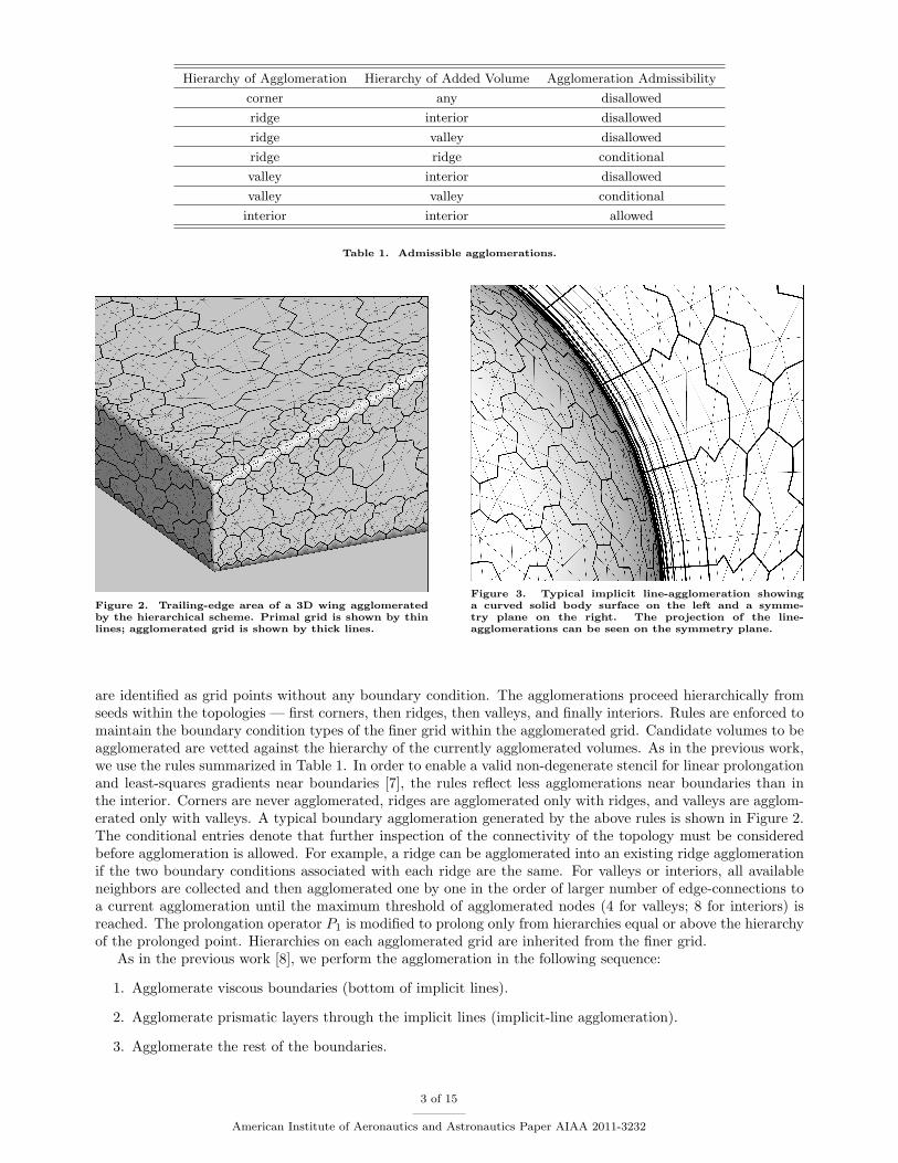
Figure 2. Trailing-edge area of a 3D wing agglomeratedby the hierarchical scheme. Primal grid is shown by thinlines; agglomerated grid is shown by thick lines.

Figure 3. Typical implicit line-agglomeration showinga curved solid body surface on the left and a symme-try plane on the right. The projection of the line-agglomerations can be seen on the symmetry plane.

are identified as grid points without any boundary condition. The agglomerations proceed hierarchically fromseeds within the topologies — first corners, then ridges, then valleys, and finally interiors. Rules are enforced tomaintain the boundary condition types of the finer grid within the agglomerated grid. Candidate volumes to beagglomerated are vetted against the hierarchy of the currently agglomerated volumes. As in the previous work,we use the rules summarized in Table 1. In order to enable a valid non-degenerate stencil for linear prolongationand least-squares gradients near boundaries [7], the rules reflect less agglomerations near boundaries than inthe interior. Corners are never agglomerated, ridges are agglomerated only with ridges, and valleys are agglom-erated only with valleys. A typical boundary agglomeration generated by the above rules is shown in Figure 2.The conditional entries denote that further inspection of the connectivity of the topology must be consideredbefore agglomeration is allowed. For example, a ridge can be agglomerated into an existing ridge agglomerationif the two boundary conditions associated with each ridge are the same. For valleys or interiors, all availableneighbors are collected and then agglomerated one by one in the order of larger number of edge-connections toa current agglomeration until the maximum threshold of agglomerated nodes (4 for valleys; 8 for interiors) isreached. The prolongation operator P1 is modified to prolong only from hierarchies equal or above the hierarchyof the prolonged point. Hierarchies on each agglomerated grid are inherited from the finer grid.

As in the previous work [8], we perform the agglomeration in the following sequence:

1. Agglomerate viscous boundaries (bottom of implicit lines).

2. Agglomerate prismatic layers through the implicit lines (implicit-line agglomeration).

3. Agglomerate the rest of the boundaries.

3 of 15

American Institute of Aeronautics and Astronautics Paper AIAA 2011-3232

4. Agglomerate the interior.

The second step is a line-agglomeration step where volumes are agglomerated along implicit lines starting fromthe volume directly above the boundary volume. Specifically, we first agglomerate volumes corresponding tothe second and third entries in the implicit-line lists associated with each of the fine-grid volumes contained ina boundary agglomerate. The line agglomeration continues to the end of the shortest line among the lines asso-ciated with the boundary agglomerate. This line-agglomeration process preserves the boundary agglomerates.Figure 3 illustrates typical implicit line-agglomeration near a curved solid body. The implicit line-agglomerationpreserves the line structure of the fine grid on coarse grids, so that line-relaxations can be performed on all gridsto address the grid anisotropy. If no implicit lines are defined, typical for inviscid grids, the first two steps areskipped.

In each boundary agglomeration (steps 1 and 3), agglomeration begins with corners (ridges or valleys ifcorners do not exist), creates a front list defined by collecting volumes adjacent to the agglomerated corners,and proceeds to agglomerate volumes in the list (while updating the list as agglomeration proceeds) in the orderof ridges and valleys. During the process, a volume is selected from among those in the same hierarchy that hasthe least number of non-agglomerated neighbors, thereby reducing the occurrences of agglomerations with smallnumbers of volumes. A heap data-structure is utilized to efficiently select such a volume. The agglomerationcontinues until the front list becomes empty. Finally, for both valleys and interiors, agglomerations containingonly a few volumes (typically one) are combined with other agglomerations.

III.B. Parallel Implementation

For parallel implementation, the hierarchical agglomeration algorithm is applied independently to each partition.That is, no agglomeration is performed across partition boundaries. In each partition, we first select a startingvolume in the priority order: corner, ridge, valley, and interior. Then, we execute the hierarchical agglomerationdescribed above within the partition. In rare cases, a partition consists of a few disjoint grids. If such a partitionis found, e.g., by a neighbor-to-neighbor search, we set up a starting volume in each disjoint grid to fullyagglomerate the partition. No special modification is necessary for the line agglomeration as our partitioningguarantees that all nodes in each implicit-line belong to the same partition. Due to the advancing-front nature ofthe agglomeration scheme, the resulting agglomerated grids will be different for different numbers of partitions.However, no significant dependence is observed in the numerical results presented in this paper. Partition-independent agglomeration remains a challenge; it is a subject of future work.

IV. Single-grid Iterations

The single-grid iteration scheme is based on the implicit formulation:(Ω

∆τ+

∂R∗

∂U

)δU = −R(U), (2)

where R(U) is the target residual computed for the current solution U , ∆τ is a pseudo-time step, ∂R∗

∂U is anexact/approximate Jacobian, and δU is the change to be applied to the solution U . An approximate solution toEquation (2) is computed by a certain number of relaxations on the linear system (linear-sweeps). Update of Ucompletes one nonlinear iteration. The RANS equations are iterated in a loosely-coupled formulation: first themean-flow variables are updated, and then the turbulence residual is evaluated and the turbulence variable isupdated. The left-hand-side operator of Equation (2) includes the exact linearization of the viscous terms anda linearization of the inviscid terms involving first-order contributions only. Thus, the iterations represent avariant of defect correction. Typically in our single-grid RANS applications, the first-order Jacobian correspondsto the linearization of Van Leer’s flux-vector splitting [17]. But the linearization of Roe’s approximate Riemannsolver is also available. In this study, Jacobians are updated after each iteration.

The linear sweeps performed before each nonlinear update include νp sweeps of the point multi-color Gauss-Seidel relaxation performed through the entire domain followed by νl line-implicit sweeps in stretched regions.The line-implicit sweeps are applied only when solving the Navier-Stokes or RANS equations. In a line-implicitsweep, unknowns associated with each line are swept simultaneously by inverting a block tridiagonal matrix [7].Our single-grid computations do not represent the default FUN3D usage; they differ in the Jacobian type andupdate strategy and the use of implicit-lines.

4 of 15

American Institute of Aeronautics and Astronautics Paper AIAA 2011-3232

V. Multigrid

V.A. Multigrid V-Cycle

The multigrid method is based on the full-approximation scheme (FAS) [1, 18] where a coarse-grid problem issolved/relaxed for the solution approximation. A correction, computed as the difference between the restrictedfine-grid solution and the coarse-grid solution, is prolonged to the finer grid to update the fine-grid solution. Thetwo-grid FAS is applied recursively through increasingly coarser grids to define a V-cycle. A V-cycle, denotedas V (ν1, ν2), uses ν1 relaxations performed at each grid before proceeding to the coarser grid and ν2 relaxationsafter coarse-grid correction. On the coarsest grid, relaxations are performed to bring two orders of magnituderesidual reduction or until the maximum number of relaxations, 10, is reached.

V.B. Inter-Grid Operators

The control volumes of each agglomerated grid are found by summing control volumes of a finer grid. Anoperator that performs the summation is given by a conservative agglomeration operator, R0, which acts onfine-grid control volumes and maps them onto the corresponding coarse-grid control-volumes. Any agglomeratedgrid can be defined, therefore, in terms of R0 as

Ωc = R0Ωf , (3)

where superscripts c and f denote entities on coarser and finer grids, respectively. On the agglomerated grids,the control volumes become geometrically more complex than their primal counterparts and the details of thecontrol-volume boundaries are not retained. The directed area of a coarse-grid face separating two agglomeratedcontrol volumes, if required, is found by lumping the directed areas of the corresponding finer-grid faces and isassigned to the virtual edge connecting the centers of the agglomerated control volumes.

Residuals on the fine grid, Rf , corresponding to the integral equation (1), are restricted to the coarse gridby the conservative agglomeration operator, R0, as

Rc = R0Rf , (4)

where Rc denotes the fine-grid residual restricted to the coarse grid. The fine-grid solution approximation, Uf ,is restricted as

U c0 =

R0(UfΩf )

Ωc, (5)

where U c0 denotes the fine-grid solution approximation restricted to the coarse grid. The restricted approximation

is then used to define the forcing term to the coarse-grid problem as well as to compute the correction, (δU)c:

(δU)c = U c − U c0 , (6)

where U c is an updated coarse-grid solution obtained directly from the coarse-grid problem. The correction tothe finer grid is prolonged typically through the prolongation operator, P1, that is exact for linear functions, as

(δU)f = P1(δU)c. (7)

The operator P1 is constructed locally using linear interpolation from a tetrahedra defined on the coarse grid.The geometrical shape is anchored at the coarser-grid location of the agglomerate that contains the given finercontrol volume. Other nearby points are found by the adjacency graph. An enclosing simplex is sought thatavoids prolongation with non-convex weights and, in situations where multiple geometrical shapes are found,the first one encountered is used. Where no enclosing simplex is found, the simplex with minimal non-convexweights is used.

V.C. Coarse-Grid Discretizations

For inviscid coarse-grid discretization, a first-order edge-based scheme is employed. For the viscous term, twoclasses of coarse-grid discretizations were previously studied [6, 7]: the Average-Least-Squares (Avg-LSQ) andthe edge-terms-only (ETO) schemes. The consistent Avg-LSQ schemes are constructed in two steps: first,LSQ gradients are computed at the control volumes; then, the average of the control-volume LSQ gradients isused to approximate a gradient at the face, which is augmented with the edge-based directional contribution

5 of 15

American Institute of Aeronautics and Astronautics Paper AIAA 2011-3232

Inviscid Viscous (Diffusion)

Primal grid Second-order edge-based reconstruction Face-Tangent Green-Gauss

Coarse grids First-order edge-based reconstruction Face-Tangent Avg-LSQ

Table 2. Summary of discretizations used to define the residual, R.

Inviscid Viscous

Primal grid Approximate (first-order scheme) Exact (R∗ = R)

Coarse grids Exact or Approximate Approximate (edge-terms only)

Table 3. Summary of Jacobians, ∂R∗∂U .

to determine the gradient used in the flux. There are two variants of the Avg-LSQ scheme. One uses theaverage-least-squares gradients in the direction normal to the edge (edge-normal gradient construction). Theother uses the average-least-squares gradients along the face (face-tangent gradient construction [7]).

The ETO discretizations are obtained from the Avg-LSQ schemes by taking the limit of zero Avg-LSQgradients. The ETO schemes are often cited as a thin-layer discretization in the literature [2, 3, 4]; they arepositive schemes but are not consistent (i.e., the discrete solutions do not converge to the exact continuoussolution with consistent grid refinement) unless the grid is orthogonal [16, 19]. As shown in the previouspapers [6, 7], ETO schemes lead to deterioration of the multigrid convergence for refined grids, and thereforeare not considered in this paper. For practical applications, the face-tangent Avg-LSQ scheme was found tobe more robust than the edge-normal Avg-LSQ scheme [8]. It provides superior diagonal dominance in theresulting discretization [6, 7]. In this study, we employ the face-tangent Avg-LSQ scheme [7] as a coarse-griddiscretization of the viscous term. It has been implemented in the form independent of the face-tangent vectors(see Appendices of Ref. [14]). For excessively-skewed faces over 90 angle between the outward face normal andthe corresponding outward edge vector, which can arise on agglomerated grids, the viscous fluxes are ignored.For inviscid discretization, we employ a first-order edge-based discretization on coarse grids. Table 2 shows asummary of discretizations used.

V.D. Relaxations

The relaxation scheme is similar to the single-grid iteration described in Section IV with the following impor-tant differences. On coarse grids, the Avg-LSQ scheme used for viscous terms has a larger stencil than theGreen-Gauss scheme implemented on the target grid and its exact linearization has not been used; instead, anapproximate linearization based on the corresponding ETO scheme is used. For the inviscid part, the first-orderJacobian is constructed based on Van Leer’s flux-vector splitting or Roe’s approximate Riemann solver in ac-cordance with the linearization employed on the target grid. If the latter is employed, the linearization will beexact on coarse grids where the first-order scheme is used for the residual.

Table 3 summarizes the Jacobians used for inviscid and viscous terms on the primal and coarse grids. TheJacobians are updated in all levels at the beginning of a cycle and frozen through the end of the cycle. Comparedwith the single-grid scheme in which the Jacobians are updated at every iteration in this study, this strategysaves a significant amount of computing time for multigrid. As in the previous work [8], significantly fewerlinear sweeps are used in a multigrid relaxation than in a single-grid iteration: typically, νp = νl = 5 for boththe mean flow and turbulence relaxations.

VI. Numerical Results

VI.A. Inviscid Flows

The multigrid method was applied to two inviscid cases: a wing-body configuration (1, 012, 189 nodes), anda wing-flap configuration (1, 184, 650 nodes). The inflow Mach number is 0.3, the angles of attack are 0.0 forthe wing-body configuration and 2.0 degrees for the wing-flap configuration. The multigrid V (2, 1) cycle of 3levels was employed for these cases, with 4, 8, 12, and 16 processors. For these inviscid cases, the full-multigrid

6 of 15

American Institute of Aeronautics and Astronautics Paper AIAA 2011-3232

Wing-Body(0.2M) Wing-Body(1.0M) Wing-Flap(1.2M)

Multigrid V(2,1) 0.400(34) 0.530(47) 0.860(66)

Single Grid 0.955(370) 0.958(680) 0.956(459)

Table 4. Asymptotic convergence rates for the inviscid case. Numbers in the parenthesis are single-grid iterations ormultigrid cycles to convergence.

algorithm was employed to obtain the initial solution on the target grid. Also, the relaxation is based on alinearization of the Roe flux in the multigrid. For linear sweeps, we set (νp, νl) = (15, 0) for the single-gridscheme, and (νp, νl) = (5, 0) for the multigrid.

The CFL number is ramped from 10 to 200 during the first 10 iterations/cycles for single-grid/multigridcalculations. All cases have been run until the residual reaches the machine zero, 10−15.

Figure 4 shows grids and results for the wing-body configuration case. The convergence results for allprocessors are given in Figure 4(d); it shows that the convergence is nearly independent of the number ofprocessors (i.e., the multigrid lines are overlapped, and so are the single-grid lines). Figure 4(e) shows theconvergence results for 16 processors. It shows that the multigrid converges 5 times faster in CPU time thanthe single-grid relaxations. A reasonable parallel scalability can be observed in Figure 4(f) where the solid linesindicate the perfect scaling. It shows also that the speed-up factor is almost independent of the number ofprocessors. Figure 5 shows convergence results for the same wing-body configuration case with two differentsizes of grids: 0.2 and 1 million grids. As can be seen in Figure 5(a), the multigrid convergence is not exactlygrid-independent, but the dependency is much weaker than the single-grid convergence dependence. Translatedinto the CPU time, it implies a substantial speed-up for larger-scale problems. Figure 5(b) shows in fact thatthe multigrid is about 2 times faster then the single-grid scheme for the 0.2-million grid, and 5 times faster forthe one-million grid.

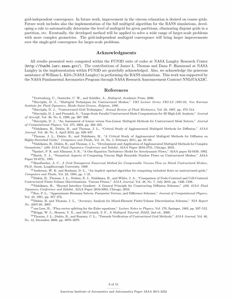
Figure 6 shows grids and results for the wing-flap configuration case. The processor-independent convergenceis demonstrated in Figures 6(d). Figure 6(e) shows that the multigrid converges nearly 3 times faster in CPUtime than the single-grid scheme. A reasonable parallel scalability is demonstrated in Figure 6(f).

In both inviscid cases, the cost of one multigrid V (2, 1) cycle is roughly equal to three single-grid iterations.Typically, one would expect that one multigrid V (2, 1) cycle is equivalent to 4 single-grid iterations. However,the multigrid requires a less number of linear-sweeps than the single-grid iteration, which can cut a significantportion of the expected cost. See Ref. [8] for a detailed cost comparison.

Asymptotic convergence rates are shown in Table 4, which are averaged rates over the last 10 cycles/iterationsand over the four-different-processor cases.

VI.B. Laminar Flow

For viscous flow applications, we encountered a significant slow down in multigrid convergence, but then foundthat additional relaxations improve the performance. We thus applied the multigrid algorithm with 3-levelV (3, 3) to a laminar flow over a hemisphere cylinder. The inflow Mach number is 0.2, the angle of attack is zero,and the Reynolds number is 400. We performed a convergence study using four different grids: 0.6, 1.4, 2.7and 4.5 million nodes. Each grid is a mixed grid with a highly-stretched prismatic grid around the hemispherecylinder and isotropic tetrahedra elsewhere. The line-agglomeration/relaxation algorithm was applied in thestretched region. For both multigrid and single-grid calculations, the CFL number is 200 and the linearization ofRoe’s approximate Riemann solver was used as a driver. The CFL number is ramped from 10 to 200 during thefirst 500 iterations for the single-grid calculations and 50 cycles for the multigrid calculations. The number oflinear point/line-sweeps is 25 for the single-grid calculations, and 10 for the multigrid calculations. The numberof processors used here is 16. The use of the linearization of the Roe flux and a larger number of linear sweepswere necessary for both schemes to converge in all cases although the single-grid scheme still fails to convergefor the finest grid.

Figure 7 shows grids and convergence results. Figure 7(d) shows the convergence results. The single-gridscheme shows a consistent increase in the number of iterations with the number of nodes. It also shows that itis non-convergent for the finest grid. On the other hand, the multigrid converged on all grids. Results in Figure7(d) indicate that the number of cycles to convergence varies slightly with the number of nodes, implying thegrid-independent convergence of the multigrid (see Table 5 for the number of cycles). In terms of CPU time,Figure 7(e) shows that the multigrid is nearly four times faster then the single-grid scheme on the grid of

7 of 15

American Institute of Aeronautics and Astronautics Paper AIAA 2011-3232

0.6M 1.4M 2.7M 4.5M

Multigrid V(3,3) 0.789(68) 0.854(107) 0.826(93) 0.820(118)

Single Grid 0.944(479) 0.967(647) 0.980(907) 1.00

Table 5. Asymptotic convergence rates for the laminar case. Numbers in the parenthesis are single-grid iterations ormultigrid cycles to convergence.

Mean flow Turbulence

Multigrid V(3,3) 0.940 0.913

Single Grid 0.980 0.996

Table 6. Asymptotic convergence rates for the RANS case.

2.7M nodes. Table 5 summarizes the asymptotic convergence rates (averaged over the last 50 cycles/iterations)observed in the numerical results. It shows that the convergence rate (per iteration) for the single grid schemedeteriorates as the grid gets finer whereas the convergence rate (per cycle) for the multigrid does not deteriorateas the grid gets finer. Finally, these results indicate that the cost of one multigrid V (3, 3) cycle is roughly equalto two single-grid iterations.

VI.C. Turbulent Flows (RANS)

We applied the 3-level V (3, 3) multigrid algorithm to a RANS simulation on the DPW-W2 grid (1.88 millionnodes), with 16, 20, and 36 processors. The inflow Mach number is 0.76, the angle of attack is 0.5 degree, andthe Reynolds number is 5 million. The initial solution is a free stream condition. For the single-grid scheme, theCFL number is ramped from 10 to 200 for the mean-flow equations and and 1 to 30 for turbulence equation overthe first 50 iterations. For the multigrid scheme, the CFL number is ramped from 10 to 500 for the mean-flowequations and 10 to 300 for turbulence equation over the first 50 cycles. The grid is, again, a mixed grid with anisotropic tetrahedral region and a highly-stretched prismatic layer around the wing. As in the laminar case, theline-agglomeration/relaxation algorithm was applied in the stretched region. In both multigrid and single-gridcalculations, the linearization of Van Leer’s flux-vector splitting scheme was used as a driver. The number oflinear point/line-sweeps is 15 for the mean-flow equations and 10 for the turbulence equation in the single-gridcalculations. For the multigrid calculations, it is 5 for the mean-flow and turbulence equations.

Grids and results are shown in Figures 8 and 9. The convergence results for all processors are given inFigure 8(d); it shows that the convergence is nearly independent of the number of processors. Figure 8(e) showsthe convergence results for 16 processors; it shows that the multigrid converges about three times as fast inCPU time as the single-grid scheme. The parallel scalability is consistent with the single-grid scheme, as canbe observed in Figure 8(f). Figures 9(a) and 9(b) show the convergence results for the turbulence equation.Again, the convergence is nearly independent of the number of processors. The speed-up factor in CPU timeis nearly 7 for the turbulence equation. Asymptotic convergence rates, obtained as averaged rates over thelast 50 cycles/iterations and over the three-different-processor cases, are given in Table 6. For this problem,the multigrid converged in 160 cycles while the single grid scheme converged in 1958 iterations. These resultsindicate that similarly to the laminar case, the cost of one multigrid V (3, 3) cycle is roughly equal to two single-grid iterations. Finally, the lift and drag coefficients are 0.4865003979 and 0.020783234900, respectively, for allcases: they are identical up to 10 and 11 significant digits, respectively.

VII. Concluding Remarks

A parallel agglomerated multigrid algorithm has been developed and applied to inviscid and viscous flowproblems over realistic geometries. A robust fully-coarsened hierarchical agglomeration scheme has been ex-tended for parallel computations. The developed method was applied to the inviscid, laminar, and RANSsimulations over realistic geometries. Numerical results show that impressive speed-ups can be achieved forrealistic flow simulations. For the viscous cases, it was found that the relaxation scheme did not provide enoughsmoothing for the multigrid to work effectively and the use of V (3, 3) (instead of V (2, 1)) greatly improved themultigrid convergence. For the laminar case, we have demonstrated that the multigrid method can achieve the

8 of 15

American Institute of Aeronautics and Astronautics Paper AIAA 2011-3232

grid-independent convergence. In future work, improvement in the viscous relaxation is desired on coarse grids.Future work includes also the implementation of the full multigrid algorithm for the RANS simulations, devel-oping a rule to automatically determine the level of multigrid for given partitions, eliminating disjoint grids in apartition, etc. Eventually, the developed method will be applied to solve a wide range of larger-scale problemswith more complex geometries. The grid-independent multigrid convergence will bring larger improvementsover the single-grid convergence for larger-scale problems.

Acknowledgments

All results presented were computed within the FUN3D suite of codes at NASA Langley Research Center(http://fun3d.larc.nasa.gov/). The contributions of James L. Thomas and Dana P. Hammond at NASALangley in the implementation within FUN3D are gratefully acknowledged. Also, we acknowledge the generousassistance of William L. Kleb (NASA Langley) in performing the RANS simulations. This work was supported bythe NASA Fundamental Aeronautics Program through NASA Research Announcement Contract NNL07AA23C.

References

1Trottenberg, U., Oosterlee, C. W., and Schuller, A., Multigrid , Academic Press, 2000.2Mavriplis, D. J., “Multigrid Techniques for Unstructured Meshes,” VKI Lecture Series VKI-LS 1995-02, Von Karman

Institute for Fluid Dynamics, Rhode-Saint-Genese, Belgium, 1995.3Mavriplis, D. J., “Unstructured Grid Techniques,” Annual Review of Fluid Mechanics, Vol. 29, 1997, pp. 473–514.4Mavriplis, D. J. and Pirzadeh, S., “Large-Scale Parallel Unstructured Mesh Computations for 3D High-Lift Analysis,” Journal

of Aircraft , Vol. 36, No. 6, 1999, pp. 987–998.5Mavriplis, D. J., “An Assessment of Linear versus Non-Linear Multigrid Methods for Unstructured Mesh Solvers,” Journal

of Computational Physics, Vol. 275, 2002, pp. 302–325.6Nishikawa, H., Diskin, B., and Thomas, J. L., “Critical Study of Agglomerated Multigrid Methods for Diffusion,” AIAA

Journal , Vol. 48, No. 4, April 2010, pp. 839–847.7Thomas, J. L., Diskin, B., and Nishikawa, H., “A Critical Study of Agglomerated Multigrid Methods for Diffusion on

Highly-Stretched Grids,” Computers and Fluids, Vol. 41, No. 1, February 2011, pp. 82–93.8Nishikawa, H., Diskin, B., and Thomas, J. L., “Development and Application of Agglomerated Multigrid Methods for Complex

Geometries,” 40th AIAA Fluid Dynamics Conference and Exhibit , AIAA Paper 2010-4731, Chicago, 2010.9Spalart, P. R. and Allmaras, S. R., “A One-Equation Turbulence Model for Aerodynamic Flows,” AIAA paper 92-0439, 1992.

10Barth, T. J., “Numerical Aspects of Computing Viscous High Reynolds Number Flows on Unstructured Meshes,” AIAAPaper 91-0721, 1991.

11Haselbacher, A. C., A Grid-Transparent Numerical Method for Compressible Viscous Flow on Mixed Unstructured Meshes,Ph.D. thesis, Loughborough University, 1999.

12Anderson, W. K. and Bonhaus, D. L., “An implicit upwind algorithm for computing turbulent flows on unstructured grids,”Computers and Fluids, Vol. 23, 1994, pp. 1–21.

13Diskin, B., Thomas, J. L., Nielsen, E. J., Nishikawa, H., and White, J. A., “Comparison of Node-Centered and Cell-CenteredUnstructured Finite-Volume Discretizations: Viscous Fluxes,” AIAA Journal , Vol. 48, No. 7, July 2010, pp. 1326–1338.

14Nishikawa, H., “Beyond Interface Gradient: A General Principle for Constructing Diffusion Schemes,” 40th AIAA FluidDynamics Conference and Exhibit , AIAA Paper 2010-5093, Chicago, 2010.

15Roe, P. L., “Approximate Riemann Solvers, Parameter Vectors, and Difference Schemes,” Journal of Computational Physics,Vol. 43, 1981, pp. 357–372.

16Diskin, B. and Thomas, J. L., “Accuracy Analysis for Mixed-Element Finite-Volume Discretization Schemes,” NIA ReportNo. 2007-08 , 2007.

17van Leer, B., “Flux-vector splitting for the Euler equations,” Lecture Notes in Physics, Vol. 170, Springer, 1982, pp. 507–512.18Briggs, W. L., Henson, V. E., and McCormick, S. F., A Multigrid Tutorial , SIAM, 2nd ed., 2000.19Thomas, J. L., Diskin, B., and Rumsey, C. L., “Towards Verification of Unstructured Grid Methods,” AIAA Journal , Vol. 46,

No. 12, December 2008, pp. 3070–3079.

9 of 15

American Institute of Aeronautics and Astronautics Paper AIAA 2011-3232

(a) Level 1: primal grid. (b) Level 2: coarse grid.

(c) Level 3: coarse grid.

Multigrid Cycles or Single Grid Iterations

Log1

0(D

ensi

tyR

esid

ual)

100 200 300 400 500 600

10-14

10-12

10-10

10-8

10-6 Multigrid (np= 4)Multigrid (np= 8)Multigrid (np=12)Multigrid (np=16)Single grid (np= 4)Single grid (np= 8)Single grid (np=12)Single grid (np=16)

(d) Convergence history (multigrid lines are over-lapped; single-grid lines are overlapped.)

CPU Time (sec)

Log1

0(D

ensi

tyR

esid

ual)

500 1000 1500 2000 2500

10-14

10-12

10-10

10-8

10-6 Multigrid (np=16)Single grid (np=16)

(e) Convergence history : residual vs. CPU time (16processors)

0.2 0.4 0.6 0.8 1 1.2 1.4 1.6

0.8

1

1.2

1.4

1.6

1.8

2

Log10

(Processors)

Log

10(C

PU T

ime

Min

utes

)

(f) Parallel Scalability (Stars for single grid; circlesfor multigrid; solid lines indicate the perfect scaling.)

Figure 4. Grids and convergence history for the wing-body inviscid case (1 million nodes).

10 of 15

American Institute of Aeronautics and Astronautics Paper AIAA 2011-3232

MG Cycles or Single Grid Iterations

Log1

0(D

ensi

tyR

esid

ual)

100 200 300 400 500 600

10-14

10-12

10-10

10-8

10-6 Multigrid (0.2M Nodes)Multigrid (1.0M Nodes)Single Grid (0.2M Nodes)Single Grid (1.0M Nodes)

(a) Convergence history

CPU Time (sec)

Log1

0(D

ensi

tyR

esid

ual)

500 1000 1500 2000 2500

10-14

10-12

10-10

10-8

10-6 Multigrid (0.2M Nodes)Multigrid (1.0M Nodes)Single Grid (0.2M Nodes)Single Grid (1.0M Nodes)

(b) Residual vs. CPU time (16 processors)

Figure 5. Convergence histories for the wing-body inviscid cases (16 processors).

11 of 15

American Institute of Aeronautics and Astronautics Paper AIAA 2011-3232

(a) Level 1: primal grid. (b) Level 2: coarse grid.

(c) Level 3: coarse grid.

Multigrid Cycles or Single Grid Iterations

Log1

0(D

ensi

tyR

esid

ual)

100 200 300 400 500

10-15

10-14

10-13

10-12

10-11

10-10

10-9

10-8

10-7 Multigrid (np= 4)Multigrid (np= 8)Multigrid (np=12)Multigrid (np=16)Single grid (np= 4)Single grid (np= 8)Single grid (np=12)Single grid (np=16)

(d) Convergence history (multigrid lines are over-lapped; single-grid lines are overlapped.)

CPU Time (sec)

Log1

0(D

ensi

tyR

esid

ual)

500 1000 1500

10-15

10-14

10-13

10-12

10-11

10-10

10-9

10-8

10-7 Multigrid (np=16)Single grid (np=16)

(e) Convergence history : residual vs. CPU time (16processors)

0.5 1 1.50.9

1

1.1

1.2

1.3

1.4

1.5

1.6

1.7

1.8

1.9

Log10

(Processors)

Log

10(C

PU T

ime

Min

utes

)

(f) Parallel Scalability (Stars for single grid; circlesfor multigrid; solid lines indicate the perfect scaling.)

Figure 6. Grids and convergence history for the wing-flap inviscid case

12 of 15

American Institute of Aeronautics and Astronautics Paper AIAA 2011-3232

(a) Level 1: primal grid. (b) Level 2: coarse grid.

(c) Level 3: coarse grid.

Multigrid cycles or Single-grid iterations

Log1

0(D

ensi

tyR

esid

ual)

200 400 600 800 100010-14

10-12

10-10

10-8

10-6

10-4Multigrid V(3,3) (0.6M nodes)Multigrid V(3,3) (1.4M nodes)Multigrid V(3,3) (2.7M nodes)Multigrid V(3,3) (4.5M nodes)Single grid (0.6M nodes)Single grid (1.4M nodes)Single grid (2.7M nodes)Single Grid (4.5M nodes)

(d) Convergence history

CPU time (sec)

Log1

0(D

ensi

tyR

esid

ual)

5000 10000 15000 20000 2500010-14

10-13

10-12

10-11

10-10

10-9

10-8

10-7

10-6

10-5 Multigrid V(3,3) (2.7M nodes)Single grid (2.7M nodes)

(e) Convergence history: residual vs. CPU time

Figure 7. Grids and convergence history for the hemisphere cylinder case (Laminar; 16 processors).

13 of 15

American Institute of Aeronautics and Astronautics Paper AIAA 2011-3232

(a) Level 1: primal grid. (b) Level 2: coarse grid.

(c) Level 3: coarse grid.

MG Cycles or Single Grid Iterations

Log1

0(D

ensi

dty

Res

idua

l)

200 400 600 80010-12

10-11

10-10

10-9

10-8

10-7

10-6

10-5

10-4

10-3

Multigrid (np=16)Multigrid (np=20)Multigrid (np=36)Single grid (np=16)Single grid (np=20)Single grid (np=36)

(d) Convergence history: density residual vs.cycle/iteration (multigrid lines are overlapped;single-grid lines are overlapped.)

CPU Time

Log1

0(D

ensi

dty

Res

idua

l)

5000 10000 15000 2000010-12

10-11

10-10

10-9

10-8

10-7

10-6

10-5

10-4

10-3

Multigrid (np=16)Single grid (np=16)

(e) Convergence history: density residual vs. CPUtime (16 processors)

1.15 1.2 1.25 1.3 1.35 1.4 1.45 1.5 1.55 1.61.6

1.8

2

2.2

2.4

2.6

2.8

3

Single grid

Multigrid

Log10

(Number of Processors)

Log

10(C

PU T

ime

Min

utes

)

(f) Parallel Scalability (solid lines indicate the per-fect scaling)

Figure 8. Grids and convergence history for the DPW-W2 case (RANS).

14 of 15

American Institute of Aeronautics and Astronautics Paper AIAA 2011-3232

MG Cycles or Single Grid Iterations

Log1

0(D

ensi

dty

Res

idua

l)

500 1000 1500 200010-12

10-10

10-8

10-6

10-4

10-2 Multigrid (np=16)Multigrid (np=20)Multigrid (np=36)Single grid (np=16)Single grid (np=20)Single grid (np=36)

(a) Convergence history: turbulence residual vs. cycle/iteration (multigridlines are overlapped; single-grid lines are overlapped.)

CPU Time

Log1

0(D

ensi

dty

Res

idua

l)

10000 20000 30000 4000010-12

10-10

10-8

10-6

10-4

10-2 Multigrid (np=16)Single grid (np=16)

(b) Convergence history: turbulence residual vs. CPU time (16 processors)

Figure 9. Convergence history of the turbulence residual in the DPW-W2 case (RANS).

15 of 15

American Institute of Aeronautics and Astronautics Paper AIAA 2011-3232