AWelfare Analysis of Hot Money∗

Alexander Guembel

Toulouse School of Economics (CRM, IDEI)

University of Toulouse 1 Capitole

Oren Sussman

Saïd Business School

University of Oxford

April 3, 2012

Abstract

There is ample evidence that cross-country contagion of financial cri-

sis is caused by short-term capital flows (hot money). It is sometimes

used in order to justify a policy of restricting the integration of the

world’s liquidity markets (fragmentation). In a model with under-

provision of liquidity, contagion and excessively-high probability of

financial crisis, we show that fragmentation has an ambiguous effect

on welfare. Indeed, we show that when a country encloses liquidity

into its own market it deprives its neighbour of liquidity, increasing

the neighbour’s probability of financial crisis. Fragmentation may

also imply that a country may “sit” on idle liquidity while its neigh-

bour suffers from a financial crisis. Hence, there are conceivable

circumstances where the welfare cost of fragmentation dominate the

benefits, giving rise to “optimal contagion” in the second-best sense.

Policy coordination plays an important role in our analysis.

∗We would like to thank Bruno Biais, Javier Suarez, Jean Tirole and seminar participants at Ban-gor Business School, ESCP Paris, and the Luxembourg School of Finance for helpful comments. Allremaining errors are ours.

Correspondence address: Oren Sussman, Saïd Business School, Oxford, OX1 1HP, UK, Tel.: +441865 288 926, e-mail: oren.sussman@sbs.ox.ac.uk

1. INTRODUCTION

The Asian Crisis convinced many that short-term capital flows, hot money, are potentially

damaging and, therefore, should be restricted. According to Bhagwati (1998) there is

“striking evidence of the inherently crisis-prone nature of free capital movements”. Calvo

(1998) coined the term “sudden stop” to describe a causal chain whereby an outflow of hot

money towards a liquidity-short foreign country can trigger a domestic financial crisis by

way of contagion. More recently, Stiglitz (2010) argued that liquidity crises “associated

with forced sales of asset ... [provides] a compelling reason that global integration may

not be desirable”. In this paper we accept that contagion should play a central role in

the analysis of hot money. At the same time we question whether it justifies a policy of

fragmentation (namely, a reversal of integration).

The reason for our skepticism is that the incidence of observed contagion needs to be

evaluated against the counterfactual of crises that could have materialized but have been

avoided due to the inflow of capital from abroad. Hence, a trade-off may exist where

more contagion in some circumstances should be tolerated for a better chance of avoiding

crisis in other circumstances, giving rise to optimal contagion (in a second-best sense).

To put it differently, by enclosing liquidity into its own market, a country may deprive

its neighbor from liquidity but, absent policy coordination, fail to internalize the welfare

implications. Hence, the old beggar-thy-neighbor effect, whereby a country attempts to

resolve domestic economic problems at the expense of its neighbor (Stiglitz, 1999) should

also play a central role in the analysis. The main question is, thus, whether a properly

modelled contagion effect is strong enough to dominate any other consideration. We

answer the question through exact welfare accounting of hot money.

To that end, we construct a two-country model where speculators invest in liquidity

in order to profit from low fire-sale prices, giving rise to a cash-in-the-market effect (as in

Allen and Gale, 1998). Fire-sales of investment goods are a direct consequence of secured

lending as in Hart and Moore (1998). Though contracts are optimally negotiated between

debtors and creditors to extract all private gains from trade (given market conditions),

bids in the fire-sale market fail to reflect the entire social value of repossessed collateral.

Hence, competitive markets are grossly inefficient, liquidity is a public good and, as such,

suffers an under-provision problem. Moreover, the competitive equilibrium captures many

stylized facts related to financial crisis: it occurs with excessively high (strictly positive)

probability and is characterized by a sharp increase in repossessions, fire sales, a drop in

investment-goods prices and credit rationing (a credit crunch). We abstract the analysis

from technological shocks; all projects are economically viable, though some may suffer

from financial distress due to a temporary shortage of income. The macro shock is

modeled as a pure redistribution of wealth within each economy, from capital-poor to

capital-rich entrepreneurs. The purpose of this abstraction is twofold: to account for

1

absent evidence that links financial crisis to any “real” factor, and to focus the analysis

on the pivotal role of liquidity.

Three results deserve special attention. First, we characterize a triage rule1, whereby

countries commit ex-ante to an allocation mechanism, contingent on the realization of

their liquidity shock. It turns out that, in some cases, it is ex-ante Pareto-optimal to

infect one country with a mild financial crisis in order to save the other from a more

serious one. Clearly, by itself, contagion is not (constrained) sub-optimal. Second, we

explore the complex externalities generated by unilateral fragmentation policies where the

government of each country encloses liquidity into its own market but ignores the effect

of the policy on its neighbor. Not only that liquidity can stand idle in one country while

the other suffers from financial crisis, the unilateral implementation of fragmentation in

one country crowds out hot money and, thus, decreases the amount of liquidity available

to its neighbor. We show that each country has the incentive to employ such beggar-thy-

neighbor policies up to the feasible maximum. Third, we show that when policies are

coordinated and cross-country externalities internalized, fragmentation can be optimal

only in some cases. Since the uncoordinated equilibrium is at full fragmentation, it

follows that there is “too much fragmentation” in an uncoordinated equilibrium.

To sum up, while our model provides strong grounds to believe that liquidity is under-

provided in a competitive equilibrium, it provides only limited grounds to believe that

a policy of fragmentation contributes to ameliorating the problem. Moreover, policy co-

ordination can mitigate the externalities associated with fragmentation and contribute

to social welfare. At a minimum, coordination should moderate the tendency towards

excessive fragmentation in an uncoordinated equilibrium. Even better, an IMF-like in-

stitution can be created, which would hold liquidity and dispatch it conditional on the

realized shocks in the two countries, resolving the commitment problems inherent in the

triage rule.2

Though we frame our research question in the context of international finance, the

analysis contributes to an understanding of a broader question: the role of markets in

providing and allocating liquidity. For example, the question whether banks should be

self-sufficient in reserve liquidity or rely on liquid markets to provide for shortages is

related in some important respects to the one that we investigate here; see also Gale and

Yorulmazer (2011). Our results seem to indicate that black-and-white, pro or anti market

formulae are overly simplistic. For the market clearly fails to provide sufficient liquidity

but, at the same time, the effect of crude quantitative restrictions is ambiguous, at best.

The paper is organized as follows: Section 2 presents the model, Section 3 analyzes

the contract, and Section 4 develops a single-country benchmark. Section 5 presents the

1The concept is taken from emergency medicine where it provides priority rules for treating patientsin trauma subject to scarce medical resources.

2Notice that the triage is ex-ante efficient, but ex-post a mildly infected country loses when its liquidityis used in order to save a more severely infected country.

2

two-country competitive equilibrium and Section 6 provides the welfare analysis. Section

7 concludes.

Literature reviewFisher (1933) provides the first academic analysis of the interrelations between market

prices, leverage and economic activity. The first formal modelling is by Bernanke and

Gertler (1989) and by Shleifer and Vishny (1992) who emphasize the fire-sale channel,

followed by Kiyotaki and Moore (1997), Suarez and Sussman, (1997) and many others.3

Allen and Gale, (1998) provide a link to the Diamond-Dybvig (1983) analysis of liquidity.

The central source of inefficiency is the pecuniary externality inflicted by liquidation

decisions, as in Bhattacharya and Gale (1987). Most of the building blocks that we use

in the construction of our single-country benchmark already appear in these papers. We

therefore focus below on contributions that are directly related to hot money, capital flow

and, therefore, to our own work.

Caballero and Krishnamurthy (2001, 2004) are among the first to extend the analysis

internationally. They model a small open economy where some assets are pledgeable as

collateral to domestic lenders but not to foreigners. A fraction of the domestic firms will

face financial distress in the interim period and will require additional funding. Though

the economy is entirely dependent on funding from abroad, there is a domestic loan

market where non-distressed firms borrow abroad and lend domestically utilizing their

advantage in handling domestic collateral. In this kind of a setting, the amount of debt

capacity that is left un-utilized ex ante in order to service interim distressed lending can

be interpreted as liquidity provision. It is shown that the competitive equilibrium is

inefficient. Moreover, an ex-ante borrowing tax can restore optimality by leaving more

capacity available for the interim market.

Mendoza (2010) and Korinek (2011a) construct DSGE models augmented by a con-

straint that limits borrowing to a fraction of the market value of the collateral. The

constraint is not derived from an explicit agency problem, yet it tightens endogenously

in response to a change market conditions. The setting is simple enough to allow for a

simulation of the model’s rich dynamics. A negative productivity shock might generate

a “feedback loop”, leading to weak demand, low investment-goods prices and, thus, a

reduction in borrowing capacity. The papers differ in focus. The first emphasizes that

equilibrium dynamics differ materially from that of an open economy with a frictionless

capital market during the (rare) events when the borrowing constraint binds. Perhaps

the most dramatic “reversal” is in the dynamics of the trade balance: instead of creating

a deficit so as to smooth out the effect of a negative productivity shock, the economy

goes into a surplus that amplifies the effect of the shock. Korinek (2011a) has an ex-

3The following is a very incomplete list of some related recent contributions: Brunnermeier andPedersen (2008), Bolton, Santos and Scheinkman (2009), Diamond and Rajan (2011), Goodhart et. al.(2012), Gorton and Huang (2004), Holmström and Tirole (1998, 2011), Lorenzoni (2008), Suarez andSussman (2007).

3

plicit welfare analysis of an exchange economy. In a competitive equilibrium, consumers

take capital-goods prices as given and, thus, fail to internalize the effect of their own

borrowing on the likelihood that the constraint may tighten. In contrast, a planner can

internalize the effect and tax the inflow of hot money. The optimal policy is to increase

the capital-import tax by 0.87% when capital imports increases by 1%,

The paper by Acharya et. al. (2010) is, in some respects, the closest to ours. Liquidity

is provided by specialized agents (called “arbitrageurs”) who profit from buying fire sales

assets. The amount of liquidity is determined endogenously. The key result is that the

competitive amount of liquidity is economically inefficient. The model is then extended

to the case of two countries. The analysis clearly identifies the possibility of contagion

across countries and provides a condition under which the equilibrium amount of liquidity

(per country) would increase as a result of a liquidity-market integration. The paper does

not provide an explicit welfare analysis of the two-country case.

Our paper differs from the above contributions in several respects. Wemodel in greater

detail the underlying agency problem. Although this complicates the analysis, we believe

it is worthwhile: first, because the interaction of incentives and market prices is at the core

of financial-crisis analysis. Second, the technical difficulties generated by the structural

assumptions, e.g. that our social-welfare problem has a strong tendency to yield a corner

solution, may be a fundamental property of crisis models. None of the papers above has

an explicit social-welfare analysis of the two-country case. Particularly, to the best of

our knowledge, there is no analysis of the interaction between the beggar-thy-neighbor

externality and contagion.4 As a result, there is no clear distinction in the literature

between the “pure” effect of fragmentation and its indirect effect on ameliorating the

under-provision of liquidity problem.

2. THE MODEL

Consider a world with four periods t = 0, ..., 3. There are two countries, i = A,B,

each with a measure-one continuum of entrepreneurs, who are the object of our welfare

accounting. There are also some speculators who reside out of these countries and are

excluded from the welfare accounting. All agents are risk neutral and maximize total

t = 3 consumption (there is no discounting).

Speculators make their decisions at t = 0. Denote by F ≥ 0 the amount of liquiditythat they provide, jointly. Liquidity is held in the form of consumption goods, which are

storable at a zero rate of return. Short positions are ruled out by the absence of t = 0

counter parties. At t = 0 (and then only) there is an alternative investment: an illiquid

asset that yields a riskless gross return, ρ0 ≥ 1, at t = 3. Speculators have sufficient

4See, however, Korinek (2011b) where overborrowing in one country can be mitigated by restrictingits capital inflows.

4

resources to satisfy any demand for liquidity (subject to profitability considerations). It

follows that the supply of liquidity is perfectly elastic at t = 0 and perfectly inelastic

thereafter. We shall interpret the free flow of liquidity across countries as hot money.

Figure 1

Time line

t=0 t=1 t=2 t=3

speculatorschoose F

countrieschoose Fis.t. Ti

opportunity cost:

projects start up

capital rich/poor shock

risk of distress realized winding up

contract is signedriskless rate:

r: repayment: collateral

default and repossession

fire-sale market opens

price:

uniformly distributed

( )iθ−1

iθ0ρ

1<w

1>nw

( )π−1

π

yq <<δ1≤β

y {Y,0}

0 {2Y,0}

1ρ

As we shall see, there is an under-provision of liquidity in a competitive equilibrium,

which gives governments a motive to provide some extra liquidity, Fi. To do so, they

borrow at market rate ρ0 at t = 0. At t = 3 the governments levy taxes and pay back

the debt. Tax distortions are convex in revenue. For simplicity we assume that there

are no tax distortions up to a point Ti, so that the marginal cost of government liquidity

up to that point is ρ0. Beyond Ti the cost of tax distortions increases to infinity. The

amount of government-supplied liquidity is common knowledge, so that the speculators

can adjust the amount of liquidity that they provide to changes in the amount that the

governments provide.

At t = 1 each entrepreneur gains access to one indivisible project, which requires an

investment of one unit of a consumption good in order to start up. Each entrepreneur

also receives an endowment of consumption goods, his capital, which he uses in order to

fund the project. As for our macro shock, in each country there is a random fraction, θi,

of capital-poor entrepreneurs with a w < 1 endowment, which is fixed and independent of

θi. All other entrepreneurs have an endowment of wni , a random variable. On aggregate,

each country has a non-random endowment capital wa,

wa ≡ θiw + (1− θi)wni = 1. (1)

5

It follows that for any realization of θi, wni ≥ 1, which makes the the capital-rich self

sufficient in funding. Hence, the θ shock is purely re-distributive with no technological

or aggregate-wealth implications. It does, however, create a strong motive for trading

funds at t = 1 as the capital-poor seek funding from the capital rich. We do not model

the redistributive shock but we have in mind sectorial capital losses due to, say, reckless

trading or faulty risk management. These are recognized to play a major role in triggering

a financial crisis. The incidence of poor capital is independent across the two countries

and is uniformly distributed on£0, θ¤×£0, θ¤. We assume that entrepreneurs cannot

insure against being capital poor.5

Financial frictions aside, all projects are economically viable: if carried to maturity

each project generates the same expected income, 2y , y > ρ0, of consumption goods.

There is, however, a risk of financial distress due to a temporary shortage of income. The

non-distress outcome occurs with a probability π, where the project generates an income

y at t = 2; at t = 3 it generates a random income in {Y, 0} with an expected value of y.The distress outcome occurs with a probability 1 − π, where the project generates zero

income at t = 2; at t = 3 it generates a random income in {2Y, 0} with an expected valueof 2y. Financial distress is idiosyncratic and independent of θi.

After one period that the consumption good is invested in the project, it is transformed

into an investment good. At that point (t = 2) a market is opened and a spot-price, qi, is

established. We also assume that once the investment good is detached from the investing

entrepreneur, it can generate only a fraction of {Y, 0} at t = 3, with an expected valueδ < y.6 That repossession destroys value plays a central role in our welfare results.

Clearly, qi cannot exceed δ: qi ≤ δ. Notice that the t = 2 investment-good price, qi,

can be perfectly anticipated at t = 1 when the macro shock, θi, is realized and observed.

Potential lenders might prefer to hoard liquidity in order to buy investment goods rather

than fund investment. Hence, an arbitrage relationship is established between the risk-

free lending rate, ρ1,i, and the price of investment goods:

ρ1,i =δ

qi. (2)

Income flows are private information to the entrepreneur who owns the project, and

as a result non-pledgeable. By that we mean that one cannot write enforceable contracts

contingent on income flows. In contrast, once consumption goods have been transformed

into investment goods (we have in mind buildings or machinery) they become pledgeable.

As we shall see, under the optimal contract a fraction βi of the investment is pledged

as collateral, which the lender has the right to repossess at t = 2 if the contracted

5This assumption is necessary for liquidity to play any role and can be justified if endowments areunobservable or if entrepreneurs are only born at t = 1. For a detailed discussion of the role of missinginsurance markets see Allen and Gale (2004) and Holmstrom and Tirole (2011).

6The assumption is shared with Kiyotaki and Moore (1997) and much of the literature building on it.

6

repayment, ri, is in default. Following repossession the entrepreneur can still operate

the remaining part of his project and collect a proportional income flow at t = 3, which

will be 2y (1− βi), in expectation. Notice that although all projects may suffer from a

temporary income shortage, only capital-poor entrepreneurs require external funding and

may thus risk repossession.

Our next assumption is similar to a cash-in-advance constraint: there is no settlement

in kind, only in terms of the liquid consumption good. Particularly, debt cannot be settled

by the transfer of investment goods. Rather, repossessed collateral needs to be auctioned

off, and then the proceeds are used in order to satisfy the lenders.7 Hence, the t = 2

market for investment goods is a fire-sale market. This assumption plays a critical role

in the analysis, as it forces the fire-sale price, qi, below δ if there is not enough liquidity

in the market.

Lastly, we assume that bidders in the fire-sale market need to submit orders and the

necessary liquidity to execute them before the t = 2 production process is completed.

As a result, t = 2 manufactured consumption goods are excluded from fire-sale auction

and only liquidity that was stocked up at t = 1 can participate. This assumption does

not change the qualitative features of our results and is made for realism. In practice we

do not observe that consumption drops significantly in order to increase liquidity supply.

This is presumably because of a combination of a concave utility function and sufficiently

strong time discounting - both of which we do not want to introduce into the model for

reasons of tractability.

3. THE CONTRACT

The analysis of this section, and the next, makes no reference to the specifics of country

A or B. For brevity, we omit the i index, from the exposition.

Our basic assumption in relation to the contract is that income flows are private

information to the borrower.8 Hence, a capital-poor entrepreneur cannot raise external

finance by pledging income flows, and has to pledge his investment good, instead. It

is also implied that the lender cannot distinguish a distressed from a non-distressed

entrepreneur, so repossession of the collateral can only be conditioned on the observable

event of default. Since investment goods lose all their value by t = 3, contracts need

to be settled by t = 2, when the threat of repossession is still effective. The attractive

property of this set of assumptions is that it yields a solution that is quite similar to a

standard, secured debt contract.

7This assumption is shared, among many others, with Allen and Gale (1998), Lorenzoni (2008),Diamond and Rajan (2011) Acharya, Shin and Yorulmazer (2011).

8Our setting is a complete contract version of Hart and Moore (1998) with no scope for contractrenegotiation. Bolton and Scharfstein (1990) use a closely related set-up to ours where instead of seizingcollateral at the interim date, a capital provider can refuse to provide continuation finance.

7

To see how that works consider, first, a non-distressed borrower with a y income at

t = 2. The threat of liquidation is effective if the entrepreneur would rather pay r than

lose the expected date-3 income associated with the collateral, βy. Hence, our incentive-

compatibility constraint is

r ≤ βy, (IC)

where β also needs to satisfy a feasibility constraint

β ∈ [0, 1] . (FC)

Subject to (IC), non-distressed borrowers repay their debt, leaving repossession off the

equilibrium path. As for a distressed borrower, income shortage forces him to default, in

spite of the heavy losses involved. Lastly, the lenders’ participation constraint needs to

be satisfied:

πr + (1− π)βq = ρ1 (1− w) . (PC)

We assume that (PC) holds with equality due to competition between lenders.

It follows that the optimal contract is an (r, β) pair that maximizes the borrower’s

consumption (at t = 3) subject to the constraints above:

maxr,β

π (2y − r) + (1− π) (1− β) 2y, (3)

s.t. (IC), (PC), (FC) .

(We deal with the entrepreneur’s participation constraint below.)

Substituting the binding (PC) into the objective function and re-arranging, we express

the final consumption of the capital-poor entrepreneur in terms of β alone:

c|w = 2y − ρ1 (1− w)− (1− π) β(2y − q). (4)

It equals gross income 2y, net of the cost of external funding, minus the dead-weight loss

of external funding, which is the probability of distress, (1− π), times the fraction of the

investment pledged as collateral, β, times the per-unit loss from fire sale (2y − q). Since

c|w is decreasing in β, the solution to the contract problem is the minimal β within the

feasible set of the program (3), namely:

Lemma 1 Let

b =ρ1 (1− w)

q (1− π) + πy. (5)

If b ≤ 1, the optimal contract is β = b; if b > 1, a capital-poor entrepreneur cannot obtain

external funding.

Proof see Appendix.

By substituting the arbitrage condition (2) into equation (5) we derive b as a function

of q alone: b (q). Notice that b is a decreasing function, which plays an important role in

8

the analysis of contagion below, for it means that the supply of fire-sales, θi (1− π) b (q)

is higher when fire-sale prices are lower. Moreover, qb (q) is also a decreasing function,

so that a lower fire-sale price increases the total value of fire-sales and the amount of

liquidity that is needed to absorb them.

Let q be the positive root of b (q) = 1, where (FC) is binding:

q =−πy +

q(πy)2 + 4 (1− π) δ (1− w)

2 (1− π). (6)

Clearly, prices cannot get lower than that for, then, by Lemma (1), no capital-poor

entrepreneur can get funding. The only way to avoid this outcome is to set the equilibrium

price at q and credit-ration some borrowers. Let μ be the probability of obtaining credit.

Clearly, if q > q, μ = 1; if q = q, μ ∈ [0, 1], to be determined endogenously in equilibrium.Notice that our assumptions do not prevent credit-rationed entrepreneurs from lending

their capital to others.

Lastly, we turn to the entrepreneur’s participation constraint. Suppose that credit is

rationed and fire-sale prices are down to q. According to equation (6), when w = 1, q

drops to zero and the risk-free lending rate, δq, tends to infinity. At such a high interest

rate entrepreneurs would prefer to lend rather than invest in their own project. Surely,

that cannot be an equilibrium. Rather, as entrepreneurs draw capital out of projects,

q increases via a lowering of w in equation (6), until equilibrium is restored. In other

words, at high levels of w project capitalization is endogenized. To avoid this problem

we show:

Lemma 2 For any combination of the technological parameters π, y and δ, there exists

a threshold w ∈ (0, 1) such that for any w < w, c|w > ρ1w.

Proof see Appendix.

We can now decompose

c|w = [2y − ρ1 − (1− π)β(2y − q)] + ρ1w.

Namely, final consumption of the capital-poor entrepreneur is made of endowment (in-

cluding interest) plus the private value of a project to a capital-poor entrepreneur (to be

distinguished from the social value of a project, to be introduced below). It follows from

Lemma 2 that given w < w the latter is positive. In fact, we use the result the other way

round: for any combination of the technological parameters π, y and δ, we still have one

degree of freedom to assume a positive private valuation and select w < w accordingly.

Hence:

Assumption 1

(2y − ρ1)− (1− π) (2y − q) > 0. (A1)

9

The assumption is not restrictive: in it’s absence, project capitalization would be

endogenized and A1 would hold with equality for high w’s, introducing two equilibrium

“regimes”, which is an analytical inconvenience. Notice that (2y − ρ1) is the private value

of a project to a capital-rich entrepreneur, which is greater than the value of a project to

the capital-poor entrepreneur and, hence, satisfies his participation constraint as well.

4. A SINGLE COUNTRY BENCHMARK

Suppose there is no cross-country interaction: whoever supplies liquidity, government

or speculators, deploys it to that country at t = 0 and is not allowed to redeploy it

later on. An active government operates like a welfare-oriented speculator: it borrows at

t = 0 and injects the liquidity ex-post at t = 1, 2, into the markets for lending and fire

sales. (Only that policy instrument is allowed.) Hence, the ex-post market functions in

the same way under competitive and government supply of liquidity. We analyze that

market first, and then compare the competitive outcome to that under a welfare-oriented

liquidity provider. With a slight abuse of notation we denote by F the aggregate amount

of liquidity, regardless of who provides it.

4.1. The ex-post market for liquidity

For any pre-determined F , the ex-post market for liquidity is an aggregation of two spot

markets: the t = 1 funding market for capital-poor entrepreneurs and the t = 2 fire-sale

market, both of which are linked via the arbitrage condition (2) and thus cleared through

a single price, q. The combined market-clearing condition for a certain realization of θ is:

F + (wn − 1) (1− θ) + θ (1− μ)w − θμ (1− w)− θμq (1− π) b (q) ≥ 0. (7)

On the supply side we have the speculators, the capital-rich entrepreneurs who supply

(wn − 1) liquidity each, and a fraction (1− μ) of the capital-poor entrepreneurs who

happen to be credit-rationed and are thus willing to lend their endowment at the market

rate. On the demand side, there are capital-poor entrepreneurs who are not credit ra-

tioned. The last term reflects the fire-sale market: there are θ capital-poor entrepreneurs,

of which a fraction μ actually get funding. Of those, a fraction (1− π) will be distressed,

so a fraction b (q) of their investment good is repossessed and auctioned off. The amount

of liquidity required to absorb the sale is q times θμ (1− π) b (q). In case there is more

liquidity available than demand, the clearing condition holds with inequality. Using (1)

we can rewrite the clearing condition (7) as

F + wa − (1− θ)− θμ [1 + q (1− π) b (q)] ≥ 0. (8)

Proposition 1 There exists an ex-post equilibrium in the market for liquidity, with three

possible regimes:

10

• If θ < Fq(1−π) , there is a unique equilibrium with excess supply of liquidity: q = δ, μ =

1.

• If Fq(1−π) ≤ θ ≤ F

δ(1−π)b(δ) , there are multiple equilibria as follows: (i) q = δ and

μ = 1, (ii) q ∈¡q, δ¢and μ = 1, (iii) q = q, μ < 1.

• If θ > Fδ(1−π)b(δ) , there is a unique equilibrium with credit-rationing: q = q, μ < 1.

In a credit-rationing equilibrium (either the second or the third regime) the amount of

credit rationing is:

μ =F + θ

θ£1 + q (1− π)

¤ . (9)

Proof see Appendix.

Figure 2 provides a diagrammatic exposition of the equilibrium and the existence

argument in Proposition (1). The supply of liquidity is perfectly elastic at the “fair”

price δ up to the point F +wa when liquidity supply is exhausted. As noted, the demand

for liquidity is decreasing in the fire-sale price, q. Three possible realizations of θ are

plotted: for the low and high realizations there is a unique equilibrium at points B and

C, respectively, while for the interim case there are multiple equilibria at points A, A0 and

A00. (Notice that points C and A00 represent the equilibrium price but not the quantity,

due to credit rationing.)

Figure 2The ex-post market for liquidity

q

liquidityF+wa

q

demand

supply

AB

A’A’’ C

δ

Since asset repossession destroys value, the equilibrium points in the interim case

are Pareto ranked: point A dominates point A0 which dominates point A00. Hence, the

government should try to coordinate expectations towards point A:

11

Proposition 2 In case of multiple equilibria, a policy that guarantees a fire-sale price

of δ eliminates the Pareto-dominated equilibrium points at a zero fiscal cost.

Proof. Let qe be the expected fire-sale price. Then, equilibrium is determined by sub-

stituting

bGR =δqe(1− w)

qe (1− λπ) + λπy

into the equilibrium condition (8). Clearly, the demand for liquidity is no longer sensitive

to the actual market price, q, and equilibrium is unique. Since qe = δ is an equilibrium,

it must be the only one. To the extent that the government guarantees a price of δ, the

guarantee-holders will not exercise them and the fiscal cost of the policy is zero. Notice

that this argument does not hold for θs where q is the unique equilibrium price.

Assumption 2 In case of multiple equilibria, the government coordinates expectations

towards the Pareto-dominating point.

It follows that there exist a unique critical point,

θ∗ =F

δ (1− π) b (δ)(10)

such that the economy is in “financial crisis” whenever θ > θ∗. Crisis is characterized by

a sharp increase in repossessions, a drop in the fire-sale price and by a “credit crunch”:

rationing, tighter collateral requirements and a higher cost of borrowing. Crisis is also

characterized by contagion, which has the most dramatic effect around the critical state,

θ∗. Just a tiny increase in the incidence of capital-poor entrepreneurs around θ∗ dra-

matically worsens the extent of repossessions for all other capital-poor entrepreneurs.

Contagion is intimately related to the negative slope of the demand for liquidity. For

once fire-sale prices start to drop, borrowers have to pledge a larger fraction of their

project as collateral, which generates even more fire sales. Another implication of the

negative slope of the demand for liquidity is a “multiplier effect”: the ratio between the

change in equilibrium magnitudes and the initial “shocks” that have generated them is

unbounded. Obviously, this characteristic is an immediate implication of a market where

both supply and demand slope in the same direction.

4.2. Competitive supply of liquidity

Suppose that only speculators provide liquidity. At t = 0, when they make their decisions,

they must realize that they would make losses in case no financial crisis develops at t = 1,

namely when θ < θ∗. To break even, the return on liquidity in crisis needs to exceed the

ex-ante cost of liquidity:

Assumption 3

ρ0 <δ

q. (A3)

12

It follows that the equilibrium probability of crisis,³1− θ∗

θ

´, is determined by the

break-even condition:

ρ0 =θ∗

θ+

µ1− θ∗

θ

¶δ

q. (11)

Given the critical θ∗, F is determined via equation (10), with the following important

implication:9

Lemma 3 The competitive-equilibrium probability of financial crisis, R, is strictly positive

at

R =ρ0 − 1δq− 1

.

Proof. Follows immediately from equation (11).

4.3. Welfare-oriented supply of liquidity

Liquidity is a public good. To substantiate this claim, we account social welfare across

various levels of liquidity, and compare the welfare-maximizing F to the competitive

one. Since competitive liquidity is characterized by a break-even condition (11), the

government does not break even when it deviates from competitive liquidity: it profits

(in expectations) when it “monopolizes” the liquidity market and loses when it provides

liquidity in excess of the competitive amount. Trading losses (profits) are funded by

taxes (transfers) which are non-distortionary up to the point T . Assume, for the time

being, that the constraint on T is not binding, i.e., the government could provide enough

liquidity F ≡ θδ (1− π) b (δ) so as to eliminate any crisis:

F ≤ T (12)

To derive the social-welfare function, SW (θ∗), we take expectations over the entre-

preneurs’ final consumption, c, conditional on liquidity, which is conveniently expressed

in terms of the critical θ∗, using equation (10). Doing so we net out all transfers across

capital-poor and capital-rich entrepreneurs, as well as the the government’s trading prof-

its and taxes. As a result, we account repossessions at their social cost, δ, rather than

their private cost q.

Denote the social value of a project in and out of financial crisis by v¡q¢and v (δ),

respectively, where

v¡q¢≡ (2y − 1)− (1− π) (2y − δ) , (13)

v (δ) ≡ (2y − 1)− (1− π) b (δ) (2y − δ) , (14)

∆ ≡ v (δ)− v¡q¢. (15)

9Notice that the probability of crisis is independent of distributional assumptions.

13

These are used in order to construct the social-welfare function and its derivative (see

Appendix for more detail):

SW 0 (θ∗) = [μ∗∆+ (1− μ∗) v (δ)]θ∗

θ+

µ1− θ∗

θ

¶μFv

¡q¢− (ρ0 − 1)Fθ∗ . (16)

where

μ∗ ≡ 1 + δ (1− π) b (δ)

1 + q (1− π)= μF + μθ. (17)

μF ≡ d (θμ)

dθ∗=

δ (1− π) b (δ)

1 + q (1− π), (18)

μθ ≡d (θμ)

dθ=

1

1 + q (1− π), (19)

Fθ∗ ≡dF

dθ∗= δ (1− π) b (δ) . (20)

The derivative (16) has quite an intuitive interpretation. The last term nets out

the marginal cost of liquidity: to move the critical state by dθ∗ takes Fθ∗ liquidity that

needs to be borrowed at market rate (ρ0 − 1). As a result, θ∗ capital-poor entrepreneurs,measured by the marginal density, 1/θ, are lifted out of crisis, which will allow them to

decrease the amount of pledged collateral from 1 to b (δ) and increase the social valuation

of their projects by ∆. That effect, however, is relevant only to the μ∗ fraction of capital-

poor entrepreneurs that were not credit rationed when the θ∗ state was in crisis. For

the 1 − μ∗ fraction of capital-poor entrepreneurs who were credit rationed the increase

in social valuation would be the entire social value of their project v (δ). But there is

an additional effect on those states of nature that remain in crisis, with a probability of³1− θ∗

θ

´. Due to the greater supply of liquidity, the incidence of credit rationing drops

by μF , which allows the respective entrepreneurs to increase their social contribution by

v¡q¢(which is less than v (δ) since collateral requirements are still 1 during a crisis).

The analysis is somewhat complicated by the fact that SW can be either convex or

concave.10 From (16) we can directly compute

SW 00 (θ∗) =1

θ

£∆+ (1− μ∗ − μF ) v

¡q¢¤. (21)

Nevertheless, in both cases (as well as in the two-country analysis below), solutions reveal

a strong tendency towards a corner solution.

Proposition 3 For a sufficiently high T such that (12) holds, the socially optimal level

of liquidity is at the corner θ∗ = θ resulting in a zero probability of financial crisis.

Proof see Appendix.

10For example, for the technological parameters y = 1.25, δ = 0.5 and π = 0.75 we get SW 00 > 0 forw = 0.2 and SW 00 < 0 for w = 0.1.

14

It follows that in a competitive equilibrium there is under-provision of liquidity and,

as a result, an excessively high probability of financial crisis. The main driver behind this

result is the stark difference between the break-even condition (11) and the first-order

condition (16). While the former is determined by the market value of the discontinued

investment goods, δ and q, the latter is determined by their (social) continuation value,

v (δ) and v¡q¢. Clearly, several missing markets distort prices away from social valuations.

Could the entrepreneur buy back the repossession rights from the creditor he would, but

a shortage of liquidity prevents him from doing so. Could he buy insurance that provides

him with liquidity in distress and facilitate the buy-back, he would, but that market is

missing as well. Indeed, could he buy insurance against being capital poor (and eliminate

the need to take secured credit) he would, but that market is also missing.

Another implication of the gross inefficiency of the competitive equilibrium is the

strong tendency of a welfare-enhancing policy to be pushed towards a corner solution.

Remember that there is no economic distress in our model, and that (up to T ) a policy

can mitigate financial distress by supporting fire-sale prices — without creating any tax

distortions. But then, if the policy generates welfare while applied on a narrow margin

(small θ∗), it would add even more value when applied on a wide margin, which generates,

in many cases, a convex welfare function and, always, a corner solution.

4.4. A mix of private and public liquidity

What happens if both speculators and government supply liquidity? Let θ∗ be the total

amount of liquidity provided jointly. There can be two equilibrium regimes:

θ∗

θ> (1−R), with no active speculators,

θ∗

θ= (1−R), with active speculators.

In the first equilibrium regime the probability of crisis is too small for speculators to

satisfy the break-even condition (11), so they do not participate. In the second, if the

government provides less liquidity than implied by θ∗, the speculators top up the gov-

ernment’s liquidity up to the point where the break-even condition (11) holds. It follows

that equilibrium liquidity is neutral in the government’s liquidity policy, or, to put it

differently:

Lemma 4 For equilibria where the speculators actively supply liquidity, an increase in

public liquidity crowds out private liquidity one-for-one.

Proof. Follows directly from Lemma 3.

At some point, however, the speculators withdraw from the market completely. That

happens when public liquidity increases θ∗ to the point where θ∗

θ> (1 − R). From

that point on, any increase in public liquidity would increase total liquidity by an equal

15

amount, with a corresponding decrease in the probability of crisis. The practical implica-

tion of Lemma 4 is that the government needs to “nationalize” the market for liquidity,

i.e., become the sole liquidity supplier, before it can have any welfare effect.

5. COMPETITIVE EQUILIBRIUM WITH TWO COUNTRIES

We now restore the country index i = A,B. We denote by Fi domestic liquidity, which

is deployed to country i at t = 0 and cannot be redeployed thereafter. As we shall

see below, Fi should be interpreted as publicly provided or at least publicly subsidized

liquidity. F is non-territorial liquidity or hot money, deployed to crisis economies only

upon the realization of (θA, θB) at t = 1. We follow the same structure of exposition as

before, starting with the ex-post market where both Fi and F are pre-determined.

5.1. The ex post market for liquidity

There are four equilibrium regimes: no crisis in either country (NC), a regional crisis in

one country only, either country A (RC−A) or country B (RC−B) and, finally, a “sys-

temic” crisis in both countries (SC). We maintain all previous assumptions, particularly

Assumption 2, so that in case of multiple equilibria expectations are coordinated towards

the Pareto-dominant one. Like before, qi = δ out of crisis and qi = q in crisis. Credit

is rationed in the latter case. We characterize the four regimes with the aid of Figure 3

that partitions the space set (θA, θB) ∈£0, θ¤×£0, θ¤accordingly.

There will be a NC equilibrium iff for both i = A,B both conditions hold:

Σiθi (1− π) δb (δ) ≤ F + ΣiFi, (22)

θi (1− π) δb (δ) ≤ F + Fi. (23)

Namely, there is enough liquidity in the world (domestic plus hot money) to satisfy the

entire demand by both countries at q = δ, subject to the additional constraint that each

country’s demand can be satisfied without the domestic liquidity of its neighbor. Like

before, it is convenient to express the equilibrium conditions in terms of critical θs. For

that purpose we define:

θ∗i ≡Fi

(1− π) δb (δ),

θ∗ ≡ F

(1− π) δb (δ),

bθ = Σiθ∗i + θ∗,

and reformulate conditions (22) and (23) :

Σiθi ≤ bθ, (NC)

θi ≤ θ∗i + θ∗.

16

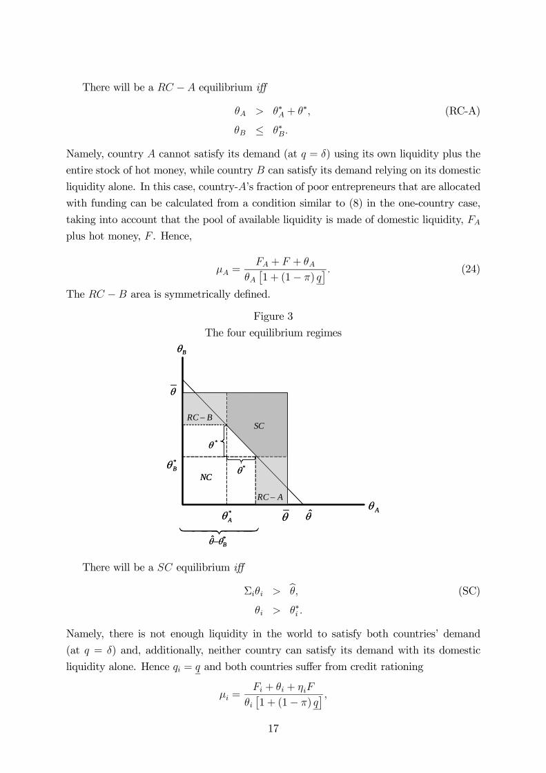
There will be a RC −A equilibrium iff

θA > θ∗A + θ∗, (RC-A)

θB ≤ θ∗B.

Namely, country A cannot satisfy its demand (at q = δ) using its own liquidity plus the

entire stock of hot money, while country B can satisfy its demand relying on its domestic

liquidity alone. In this case, country-A’s fraction of poor entrepreneurs that are allocated

with funding can be calculated from a condition similar to (8) in the one-country case,

taking into account that the pool of available liquidity is made of domestic liquidity, FA

plus hot money, F . Hence,

μA =FA + F + θA

θA£1 + (1− π) q

¤ . (24)

The RC −B area is symmetrically defined.

Figure 3

The four equilibrium regimes

*θ

*θ

*Aθ θ̂

*ˆBθθ−

θ

θ

Aθ

Bθ

*Bθ

BRC −

ARC −

NC

SC

*θ

*θ

*Aθ θ̂

*ˆBθθ−

θ

θ

Aθ

Bθ

*Bθ

BRC −

ARC −

NC

SC

There will be a SC equilibrium iff

Σiθi > bθ, (SC)

θi > θ∗i .

Namely, there is not enough liquidity in the world to satisfy both countries’ demand

(at q = δ) and, additionally, neither country can satisfy its demand with its domestic

liquidity alone. Hence qi = q and both countries suffer from credit rationing

μi =Fi + θi + ηiF

θi£1 + (1− π) q

¤ ,17

where η ≡ ηA is the share of hot money allocated to country A, and ηB = 1 − η is

allocated to country B.

So far, our assumptions impose no structure on η apart from the obvious 0 ≤ η ≤ 1.We therefore assume a simple linear allocation rule

Assumption 4 A countries’ share in hot money is proportional to the excess of domestic

demand to domestic supply of liquidity:

η

1− η=

θA − θ∗AθB − θ∗B

. (A4)

Solving for η we get:

η =θA − θ∗A

(θA − θ∗A) + (θB − θ∗B). (25)

Notably, a country’s allocation of hot money is increasing in its own excess demand and

decreasing in its neighbor’s excess demand. In the analysis below we shall give special

attention to the allocation of hot money on the margins of the SC area.

η =

⎧⎪⎪⎨⎪⎪⎩0 when θA = θ∗A (on the RC −B edge)

θA−θ∗Aθ−(θ∗A+θ∗B)

when θB = bθ − θA (on the NC edge)

1 when θB = θ∗B (on the RC −A edge)

.

Figure 4 plots the η function over the SC region for the case of symmetric supply of

domestic liquidity, namely θ∗A = θ∗B.

Figure 4

The η function with symmetric domestic liquidity

θ = 0.6, bθ = 0.5, θ∗A = θ∗B = 0.15

θ

0*Bθ

*Aθ

21

η

θ

0*Bθ

*Aθ

21

η

18

Using the characterization (NC), (RC-A) and (SC) of the regions for the various

equilibrium regimes, we can calculate their respective probabilities:

πNC =1

θ2

∙³bθ − θ∗B

´³bθ − θ∗A

´− 12

³bθ − θ∗A − θ∗B

´2¸, (26)

πRC−A =1

θ2

³θ − bθ + θ∗B

´θ∗B, (27)

πRC−B =1

θ2

³θ − bθ + θ∗A

´θ∗A, (28)

πSC =1

θ2

∙¡θ − θ∗A

¢ ¡θ − θ∗B

¢− 12

³bθ − θ∗A − θ∗B

´2¸. (29)

Since the object of our analysis is the welfare effect of hot money we restrict attention to

equilibria where speculators actively supply hot money so that θ∗ > 0. As we shall see

below, our analysis is meaningful only for equilibria where changes in hot money affect

the likelihood of both systemic and regional crisis. To that end, we also restrict attention

to equilibria where regional crisis occurs with a positive probability. Hence, for country

A, θ − (θ∗A + θ∗) > 0. It is convenient to express the above two conditions in terms of

total liquidity, bθ rather than hot money, θ∗. Hence, we restrict attention to the “relevantarea” as defined below:

Definition 1 The “relevant area” is the set of all³θ∗A, θ

∗B,bθ´ combinations such that

bθ − (θ∗A + θ∗B) > 0, (D.1)

θ −³bθ − θ∗i

´> 0. (D.2)

5.2. Competitive supply of liquidity

Since hot money can be deployed in both countries, speculators profit when at least one

country is in crisis. It follows that, given θ∗A and θ∗B, speculators select the amount of hot

money such that

πC = R, (30)

where

πC ≡ πSC + πRC−A + πRC−B. (31)

The two-country case differs materially from the one-country case in that domestic

and international liquidity are not perfect substitutes: just notice that the rate of re-

turn on hot money is πC³δq− 1´while the rate of return on domestic, say country A,

liquidity is only¡πSC + πRC−A

¢ ³δq− 1´. Clearly, domestic liquidity cannot be compet-

itively supplied. Hence, the most straight-forward interpretation of domestic liquidity is

government-supplied liquidity, with trading losses funded by taxes. Alternatively, one

19

may think of private supply of domestic liquidity, say by big domestic financial institu-

tions, where the low rate of return is compensated by some commercial advantages, say,

monopoly rights in the supply of certain financial services. These should be considered

as an effective tax on the domestic population. Or, one can interpret domestic liquidity

as being supplied by domestic speculators who are barred from speculating abroad, in

which case the tax falls on these speculators rather than the general population.

The key economic implication of imperfect substitutability is that domestic liquidity

crowds out international liquidity, but only partially so. To demonstrate the result,

substitute (27)-(29) into (31):

πC = 1− 12

⎡⎣Ãbθθ

!2−µθ∗Aθ

¶2−µθ∗Bθ

¶2⎤⎦ , (32)

and then (30) into (32). Solving for bθg (θ∗A, θ

∗B) =

qθ∗2A + θ∗2B + 2θ

2(1−R), (33)

we derive g (θ∗A, θ∗B), the competitive-equilibrium amount of total liquidity.

It follows that∂g (θ∗A, θ

∗B)

∂θ∗i=

θ∗ig (θ∗A, θ

∗B)

, for i = A,B, (34)

which allows for the characterization of partial crowding out.

Lemma 5 Suppose hot money is determined in a competitive equilibrium, so that bθ isgiven by (33). Then a unilateral increase in, say, country A’s domestic liquidity, θ∗A(holding country-B’s domestic liquidity, θ∗B, constant), i) crowds out international liquid-

ity, θ∗ but ii) only partially (i.e. by less than the increase in θ∗A), so that iii) the pool of

liquidity available to country A, θ∗A+θ∗ = bθ− θ∗B, increases, while iv) the pool of liquidity

available to country B (i.e. θ∗B + θ∗ = bθ− θ∗A) decreases. v) If at a symmetric point,

θ∗A = θ∗B, both countries increase domestic liquidity by the same amount, bθ increases.Proof. Using assumption (A5.1) in equation (34) it follows that

0 ≤ ∂g (θ∗A, θ∗B)

∂θ∗i≤ 12

for i = A,B,

from which points i)-iv) follow. Point v) follows from

0 ≤ ∂g (θ∗A, θ∗B)

∂θ∗A

¯̄̄̄θ∗A=θ

∗B

+∂g (θ∗A, θ

∗B)

∂θ∗B

¯̄̄̄θ∗A=θ

∗B

≤ 1. (35)

To gain some insight into Lemma 5 suppose, by way of contradiction, that there is full

crowding out: in Figure 3 this would correspond to increasing country-A’s liquidity, θ∗A

20

(leaving θ∗B constant), and decreasing hot money, θ∗, by the same amount, so that total

liquidity, bθ, remains the same. Clearly, the RC−B area, which represents the probabilityof country-B regional crisis, expands as the pool of liquidity available to it, θ∗B+ θ∗, falls.

It follows that the probability of crisis anywhere in the world has actually increased, which

provides speculators with an incentive to increase their supply of liquidity. It follows that

in equilibrium (after the adjustment) hot money, θ∗, falls by less than the increase in θ∗A.

Hence, the pool of liquidity available to country A, θ∗A+θ∗ = bθ− θ∗B, would increase while

the pool of liquidity available to country B, θ∗B + θ∗ = bθ− θ∗A, decreases.

To summarize the results we provide, in Figure 5, a diagrammatic illustration of

the competitive, symmetric, equilibrium. The shaded area is where conditions (D.1) and

(D.2) in Definition 1 hold. TheB−A curve plots the equilibrium amount of total liquidity,bθ, as a function of domestic (symmetric) liquidity, namely the g (θ∗A, θ∗B) function as

defined in (33). Notice that at zero domestic liquidity, total liquidity is bθ = θp2 (1−R).

Point v) of Lemma 5 demonstrates that the slope of the B−A curve is smaller than one,

so that for a B point below θ (namely R ≥ 12) the B−A curve lies within the shaded area

and intersects with its lower boundary. (Points C and D in Figure 5 are for subsequent

reference.)

Figure 5

The “relevant area”, total liquidity and symmetric-regional liquidity

θ2**BA θθ =

θ2

θ̂

( )( ) BR =−12,0 θ

A

T

C

D

*2ˆAθθ =

*ˆAθθθ +=

θ2**BA θθ =

θ2

θ̂

( )( ) BR =−12,0 θ

A

T

C

D

*2ˆAθθ =

*ˆAθθθ +=

For reasons of tractability we limit the analysis, from now on, to the symmetric case.

We also bring back the constraint on government borrowing, Ti, which until now did not

play any role in the analysis.

21

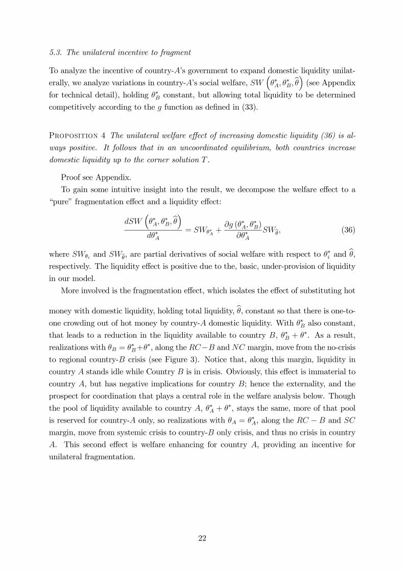
5.3. The unilateral incentive to fragment

To analyze the incentive of country-A’s government to expand domestic liquidity unilat-

erally, we analyze variations in country-A’s social welfare, SW³θ∗A, θ

∗B,bθ´ (see Appendix

for technical detail), holding θ∗B constant, but allowing total liquidity to be determined

competitively according to the g function as defined in (33).

Proposition 4 The unilateral welfare effect of increasing domestic liquidity (36) is al-

ways positive. It follows that in an uncoordinated equilibrium, both countries increase

domestic liquidity up to the corner solution T .

Proof see Appendix.

To gain some intuitive insight into the result, we decompose the welfare effect to a

“pure” fragmentation effect and a liquidity effect:

dSW³θ∗A, θ

∗B,bθ´

dθ∗A= SWθ∗A +

∂g (θ∗A, θ∗B)

∂θ∗ASWθ, (36)

where SWθi and SWθ, are partial derivatives of social welfare with respect to θ∗i and bθ,

respectively. The liquidity effect is positive due to the, basic, under-provision of liquidity

in our model.

More involved is the fragmentation effect, which isolates the effect of substituting hot

money with domestic liquidity, holding total liquidity, bθ, constant so that there is one-to-one crowding out of hot money by country-A domestic liquidity. With θ∗B also constant,

that leads to a reduction in the liquidity available to country B, θ∗B + θ∗. As a result,

realizations with θB = θ∗B+θ∗, along the RC−B andNC margin, move from the no-crisis

to regional country-B crisis (see Figure 3). Notice that, along this margin, liquidity in

country A stands idle while Country B is in crisis. Obviously, this effect is immaterial to

country A, but has negative implications for country B; hence the externality, and the

prospect for coordination that plays a central role in the welfare analysis below. Though

the pool of liquidity available to country A, θ∗A + θ∗, stays the same, more of that pool

is reserved for country-A only, so realizations with θA = θ∗A, along the RC − B and SC

margin, move from systemic crisis to country-B only crisis, and thus no crisis in country

A. This second effect is welfare enhancing for country A, providing an incentive for

unilateral fragmentation.

22

More formally, evaluating SWθ∗A at the symmetric point θ∗A = θ∗B, we can write (see

Appendix for the technical details):

SWθ∗A

³θ∗A, θ

∗B,bθ´ =

1

θ[μ∗∆+ (1− μ∗) v (δ)]

⎡⎣θ∗Aθ −³bθ − θ∗A

´θ

⎤⎦ (37)

+

∙1

2πSC +

³bθ − 2θ∗A´ ηθ∗A¸μFv ¡q¢+

∙1

2πSC −

³bθ − 2θ∗A´ ηθ∗A + πRC−A¸µ

δ

q− 1¶Fθ∗

− (ρ0 − 1)Fθ∗ +1

2Lθ∗A

³θ∗A, θ

∗B,bθ´ ,

where η is the expected value of η over the SC equilibrium regime and ηθ∗A denotes its

partial derivative with respect to θ∗A (both derived and stated in the Appendix). The

function L³θ∗A, θ

∗B,bθ´ and its partial derivative Lθ∗A are defined in the Appendix; its

economic interpretation is discussed in detail in the next section.

More accurately, on the first line of equation (37), and conditional on the marginal

realization θ∗A, the probability of crisis drops fromhθ −

³bθ − θ∗A

´i/θ to zero. To get

the (positive) welfare effect, multiply by [μ∗∆+ (1− μ∗) v (δ)], already interpreted in

relation to equation (16). The second line of (37) captures the effect of credit rationing.

The actual allocation of liquidity to country A is its own, plus its share of hot money:

θ∗A + η³bθ − θ∗A − θ∗B

´. In the RC − A region, η = 1; with full crowding out (namely

the boundary of the RC − A and the SC areas), it is still the case that η = 1, so the

substitution of hot money by domestic liquidity has no effect on credit availability. But

within the SC region, η = 12, so domestic liquidity only half crowds-out hot money,

increasing credit availability. On top, we add the (negative) effect that as country A

moves away from the symmetric point, it competes less aggressively for its share in hot

money; hence ηθ∗A. To get the welfare effect, multiply by μFv¡q¢, also interpreted in

relation to equation (16). The next line captures the effect of lower trading losses (to

speculators) as a result of the fall in hot money. Also, by being less aggressive on its

share in hot money, country A saves on trading losses, which has a positive welfare effect.

The last line captures the increase in the direct cost of liquidity.

6. WELFARE ANALYSIS OF THE TWO-COUNTRY CASE

It is already clear from the discussion above that in the case of a unilateral expansion of

liquidity, country A deprives country B from liquidity without internalizing the welfare

effect. Obviously, as countryB responds in kind it inflicts the same “beggar-thy-neighbor”

externality on country A. Clearly, the prospects of coordination should play a central

role in our welfare analysis.

Once coordination is considered, the issue of conditioning the allocation of liquidity

23

on the realized shocks (θA, θB) arises. Rather than setting aside liquidity that can be de-

ployed only domestically, the countries could agree to pool their resources and negotiate,

to their mutual benefit, a conditional allocation rule. Section 6.1 deals with this issue

and derives the triage. The analysis highlights that this optimal allocation rule requires

a degree of commitment that is not readily available among sovereigns. This may ex-

plain why the triage is not observed in practice. We therefore investigate, in Section 6.2,

whether unconditional coordination can enhance welfare.

In both these sections, and in order to allow for a meaningful analysis of fragmen-

tation out of the competitive equilibrium, one has to allow for non-regional liquidity,bθ−(θ∗A + θ∗B), which may differ from the competitive level of hot money, g (θ∗A, θ

∗B). Since

competitive hot money is defined by the break-even condition (11), it follows that there

will be non-zero trading profits, or losses (in expectation), on the non-competitive pooled

liquidity, which will have to be funded by the participating countries. To that end, and

as part of their coordination (whether conditional or unconditional), the countries would

have to set up a joint liquid fund, and deal with the trading losses (or profits) via lump-

sum taxes. We denote the expected net payoff on that fund by L³θ∗A, θ

∗B,bθ´. This term

already appears in the derivative of the welfare function (37). Since, by construction,

L [θ∗A, θ∗B, g (θ

∗A, θ

∗B)] = 0, it played only a technical role there in facilitating the decom-

position of the total effect to the liquidity and the fragmentation effects. We conclude

with a welfare analysis of unilateral fragmentation.

6.1. Coordinated state-contingent allocation of liquidity: The triage

Suppose that the two governments agree, ex ante, a certain amount of a joint liquid fund

of a magnitude bθ (to which they contribute equally) and an allocation rule contingentupon the realization (θA, θB), so as to maximize their expected welfare.

Proposition 5 Under the optimal triage rule, both countries should avoid crisis if fea-

sible, i.e., if

θA + θB ≤ bθ.There should be a country-B regional crisis, with Country A getting just enough liquidity

to avoid crisis

if θi ≤ bθ, and θA > θB,

or if θA ≤ bθ and θB > bθ.There should be a symmetric country-A regional crisis

if θi ≤ bθ, and θA < θB

or if θA > bθ and θB ≤ bθ.24

There should be a systemic crisis only when it is not feasible to contain crisis regionally,

i.e., when θA > bθ and θB > bθ. In this case the allocation of liquidity does not matter.Proof see Appendix.

Figure 6 provides a diagrammatic exposition of the triage rule. For realizations in the

NC area there is enough liquidity to rescue both countries. For realizations in the SC

area there is not enough liquidity to rescue either country. For all other realizations there

is enough liquidity to rescue only one country. Since the social cost of crisis increases

in the number of capital-poor entrepreneurs, rescue should be prioritized, with the more

badly-injured (higher θ) country coming first. Hence, in areas b1 and b2, where θA > θB

country A should be saved, leaving country B “to sink” (but still, directing towards

country B all the liquidity that is not used in the rescue of country A so as to avoid

credit-rationing as much as possible). In areas a3 and a4 although it is still the case that

θA > θB, country A cannot be saved even if it received the entire available liquidity. Only

in that case should country B, which is less badly-injured than country A be rescued,

leaving country A to its fate. A symmetric argument applies when θA < θB.

Figure 6

Crisis areas for the triage, given bθ

θ̂ θ

θ

Aθ

Bθ

SCθ̂

1n

2n

3n

2a 1a

1b

2b

3b 4b

3a

4a { }{ }{ }4321

4321

321

,,,,,,

,,

bbbbBRCaaaaARC

nnnNC

=−=−

=

θ̂ θ

θ

Aθ

Bθ

SCθ̂

1n

2n

3n

2a 1a

1b

2b

3b 4b

3a

4a { }{ }{ }4321

4321

321

,,,,,,

,,

bbbbBRCaaaaARC

nnnNC

=−=−

=

To some extent, the welfare implications of an unconditional policy can be analyzed in

terms of deviation from the triage. To that end, we compare, in Table 1, the triage with

two extreme cases of unconditional arrangements (with the same bθ): full fragmentationwhere all the available liquidity is regionalized, θ∗A = θ∗B =

bθ/2, and complete poolingwhere all liquidity is pooled, θ∗A = θ∗B = 0 and θ∗ = bθ (and allowed to flow freely, expost).

25

Table 1

Crisis regimes under the triage and unconditional fragmentation

Area Triage Unconditional fragmentation Unconditional pooling

NC {n1, n2, n3} n1 {n1, n2, n3}RC −B {b1, ...b4} {n2, a2, b3} −RC −A {a1, ..., a4} {n3, b2, a3} −SC SC {a1, a4, b1, b4, SC} {a1, ..., a4, b1, ..., b4, SC}The main advantage of an unconditional pooling policy is that it avoids the idle-

liquidity problem, as it implements the triage for realizations in areas n2 and n3. In

contrast, under fragmentation, liquid funds stand idle in one country while the other

suffers from a financial crisis. If the crisis country could draw on the liquidity of its

neighbor it would avoid crisis without infecting it.

The main advantage of an unconditional fragmentation policy is that it avoids con-

tagion from a badly-injured country to mildly-injured country, in those cases where such

contagion could not save the badly-injured country, namely for realizations in areas b3and a3. This is not the case under a pooling policy, where these areas are affected by

a systemic crisis. Evidently, there is a trade-off between resolving contagion and the

idle-liquidity problem.

For realizations in areas b2 and a2 the triage prescribes that contagion does occur

from the badly-injured country to the mildly-injured country when such contagion can

save the badly-injured country from financial crisis. This is in spite of the fact that

if the mildly injured country keeps its share in the joint liquid fund to itself, it could

avoid crisis altogether. This is a dramatic demonstration that, by itself, contagion has no

welfare implications. Contagion may well be optimal — in the second-best sense. Neither

unconditional fragmentation nor unconditional pooling implements this prescription of

the triage.

The analysis of the b2 and a2 areas highlights the commitment problem that un-

dermines the practical implementation of the triage. For in these areas, in return for

“sacrificing itself” to save its neighbor in an a2 realization, country A gets the commit-

ment that country B would act in a similar manner in a b2 realization. Hence, country

A trades away a severe crisis (high θA realization) for a milder one (low θA realization),

which is an ex-ante Pareto improvement. Since θA and θB are observable, one could imag-

ine an implementation of the triage through an international contract between country A

and country B, contingent upon (θA, θB). Given that such a contract would be written

between sovereign countries, enforcement problems are likely to be severe, particularly in

the “sacrificing” case. This may explain why triage-like policies are not observed in real-

ity. Notice, however, that a contract may be facilitated by an international organization

like the IMF, to which both countries hand over their liquidity ex ante, with full control

over the allocation of that liquidity, ex post.

26

6.2. Coordinated unconditional fragmentation

We now consider the case where countries cannot commit to a triage rule, but can agree

a coordinated move away from fragmentation (if doing so enhances ex ante welfare). We

believe that it is realistic to assume that countries could commit to such an agreement:

erecting barriers to capital flows requires structural changes in terms of monitoring, tax-

ation and enforcement that cannot be accomplished in a short period of time. Hence, if a

commitment to a certain degree of integration is made, it will be difficult to reverse on a

short notice; more so as the incentive to reverse depends on the realization of the shocks

θA and θB — see the triage analysis above. We also generalize the example of Table 1 by

considering the entire range between full fragmentation and complete pooling and prove

that the coordinated (unconditional) optimum is, indeed, at a corner. We maintain that

the total amount of liquidity can be fixed (by setting up a joint liquid fund). The analysis

is thus similar to that of the pure fragmentation effect in equation (37), only that we add

the effect of changes in country-B’s liquidity on country-A’s welfare. Due to the fixed bθ(corresponding to a move along horizontal lines in Figure 5, one of which is the dashed

C −A line), the expression is actually simpler. Hence (see Appendix for more detail):

SWθ∗A

³θ∗A, θ

∗B,bθ´+ SWθ∗B

³θ∗A, θ

∗B,bθ´

=1

θ[μ∗∆+ (1− μ∗) v (δ)]

⎡⎣θ∗Aθ −³bθ − θ∗A

´θ

−³bθ − θ∗B

´ θ∗Bθ

⎤⎦ (38)

−πRC−Av¡q¢μF .

As θ∗A and θ∗B increase simultaneously, a systemic crises becomes less likely as it is

substituted by regional crises. At the same time the probability of having no crisis also

decreases, again due to the increased likelihood of regional crises. This can be seen

graphically in Figure 3, where the effects are captured by an expansion of the RC − B

and RC −A areas into the SC and NC areas.

The interpretation of equation (38) is similar to that of equation (37) above. Coun-

try A benefits from decreasing the probability of crisis at the marginal state θ∗A byhθ −

³bθ − θ∗A

´i/θ. At the same time, it suffers from the externality imposed by country

B whereby at the marginal state³bθ − θ∗B

´the probability of crisis increases by θ∗B/θ. Fi-

nally, the last term in equation (38) captures the changes in credit rationing. Remember

that the pool of liquidity available to country A is θ∗A+η³bθ − θ∗A − θ∗B

´. In the SC area,

η equals, on average, to 1/2. Hence, the increase in both countries’ domestic liquidity

has no effect on credit availability. At the same time, in the RC −A area, η = 1 for any

realization of (θ∗A, θ∗B). It follows that the symmetric increase in both countries’ domestic

liquidity actually increases the incidence of credit rationing. Since bθ is held constant, anychanges in capital gains on the joint fund cancel against changes in the funding costs; for

more detail see Appendix.

27

An immediate implication of equation (38) is that for bθ > θ (and within the relevant

range — the shaded area in Figure 5) SW is (weakly) decreasing in fragmentation. To see

that, notice thathθ −

³bθ − θ∗A

´−³bθ − θ∗B

´i< 0 for bθ > θ and θ∗A + θ∗B < bθ. Otherwise,

Proposition 6 demonstrates that SW is U-shaped (but flattens towards the left side).

Both ways, optimal fragmentation has a corner solution. Yet, we provide an analysis of

the global maximum: a condition (in terms of a bθ threshold) for which the left end of afixed-bθ curve is higher than its right end (on the boundary of the relevant area), like theC −A curve in Figure 7.

Proposition 6 Let

ξ ≡∆+ (1− μ∗ − μF ) v

¡q¢

μ∗∆+ (1− μ∗) v (δ)< 1.

For a given level of total liquidity, bθ, the solution to the optimum, symmetric, frag-mentation is pushed to the boundary of the “relevant area” as in Definition 1, namely

θ∗A = θ∗B =bθ/2 if bθ < 3

2

ξ

1 + ξθ (39)

hold and full sharing (θ∗A = θ∗B = 0) otherwise. Moreover, ξ > 0 for a non-empty para-

meter set.

Proof see Appendix.

6.3. A welfare analysis of unilateral fragmentation with a binding T

Given our results so far, it is relatively straightforward to prove the next proposition, in

a sense our main result, implying that there is “too much fragmentation” in an unco-

ordinated equilibrium where governments make unilateral fragmentation decisions. By

Proposition 4, in absence of coordination the governments would increase local liquidity

up to the point where the T -constraint binds (within the relevant area). On the other

hand, if countries could coordinate, they would sometimes prefer to pool liquidity, rather

than to fragment markets (see Proposition 6). To complete the argument, we need to ac-

count for the negative effect of decreased fragmentation on the total amount of liquidity,bθ. This is done in the following Proposition.Proposition 7 Under coordination countries sometimes choose not to fragment, but to

pool liquidity instead.

Proof see Appendix.

28

Figure 7

SW along Figure-5 paths, when Proposition 6 is satisfied

**BA θθ =

SW

A

C

B

T**BA θθ =

SW

A

C

B

T

To gain a better insight into the argument, consider Figure 7, again. The B−A curveplots social welfare along a symmetric, competitive, equilibrium with bθ = g (θ∗A, θ

∗B). The

C −A curve is a member of a family of equal-bθ curves; in this particular case, bθ is at thelevel where hot money is just fully crowded out (see the corresponding points C −A line

in Figure 5). Moreover, the condition in Proposition 7 is satisfied, so that the C-end is

higher than the A-end of the curve. Now suppose that the countries agree a coordinated

elimination of fragmentation but, also, they agree to keep on contributing to a joint liquid

fund what they have previously contributed to their own domestic liquidity. If the T -

constraint is close enough to point A, that means moving to the left, along another equal-bθ curve, but slightly lower than the C −A curve. By the continuity of the SW manifold,

that would give them a welfare level “a bit” below point C, but still above point A.

Hence, there are cases where the uncoordinated equilibrium is at full fragmentation, but

the coordinated equilibrium is at zero fragmentation. In that respect, there is “too much

fragmentation” in an uncoordinated equilibrium.

7. CONCLUSION

Financial crisis, contagious across countries, is a market failure on a macro scale. Some

economists and policy makers have therefore concluded that avoiding contagion by re-

stricting international (short term) capital flows would be socially desirable. We argue

that this view is overly simplistic. While market fragmentation ameliorates the conta-

gion problem, it results in an inefficient use of liquidity. We show that while operating

unilaterally, countries accumulate domestic liquidity in order to protect themselves from

contagion, but in doing so they ignore the negative externality that they exert on their

29

neighbours; hence the old beggar-thy-neighbor problem in economic policy arises.

Our theoretical analysis demonstrates that there is no a-priori reason to believe that

the positive welfare effects of fragmentation generically dominate the negative effects.

It follows that decentralizing the decision over the amount of domestic liquidity and its

mobility may end in a sub-optimal equilibrium. Instead, we suggest a role for policy

coordination. In its crudest form this could be through coordinating ex ante whether to

restrict capital flows. Ideally countries should coordinate an a more refined arrangement,

whereby the allocation of liquidity is not carried out by market forces, but through a

contingency rule, similar to the triage in emergency medicine. To overcome commitment

problems, we suggest a role for an independent, international organization (say, the IMF)

that can take a decision to ex-post “sacrifice” one country in order to save another.

Our analysis considers two instruments only: fragmentation and liquidity injection.

It calls for further research into the operation of other instruments that may relieve the

problem of liquidity under-provision, yet avoid a more severe idle-funds or crowding-out

problem.

8. APPENDIX

Proof of Lemma 1. It follows from the discussion of (4) that the solution of the

contracting problem is the minimal β within the problem’s feasible set. The graph of

(PC) is a downwards-sloping line in the (r, β) space; (IC) is represented by the area

above an upwards-sloping line in the same space. Hence, the minimal point that satisfies

both (IC) and (PC) is the intersection point between the two lines given by the binding

(PC) and (IC). That point is defined by equation (5). If b ≤ 1, then (5) also defines theoptimal contract; if b > 1 the feasible set is empty and the entrepreneur cannot obtain

any funding.

Proof of Lemma 2. Let q be a fire-sale price that satisfies both b = 1 and and

c|w = ρ1w. By (IC) r = y when β = 1, which implies that c|w = πy. Hence, q must

satisfy

wδ

q= πy.

Substituting this expression into the binding (PC) at the contract β = 1, r = y and

solving for q yields

q =−πy +

q(πy)2 + (1− π) δ

(1− π).

Define z (w) ≡ q − q, where

z (w) =1

(1− π)

"πy

2+

r³πy2

´2+ (1− π) δ (1− w)−

q(πy)2 + (1− π) δ

#.

30

It is easy to verify that z (w = 0) > 0 and z (w = 1) < 0. Moreover, z (w) is continuous

and strictly decreasing in w. It follows that there is a unique w such that z¡w¢= 0 and

z¡w < w

¢> 0 (i.e., q < q). Finally, q < q implies c|w > ρ1w since q is decreasing in w

and ρ1 decreasing in q.

Proof of Proposition 1. Substituting wa = 1 into the market clearing condition (8)

and evaluating at q = δ, μ = 1 yields

F − θδ (1− π) b (δ) ≥ 0.

When this condition holds, there is enough liquidity to absorb fire sales and fund all the

entrepreneurs (μ = 1), even when the price of investment goods is bid up to their fair

value q = δ. When this condition fails to hold, and since qb (q) is decreasing in q, the

market-clearing condition (8) cannot hold with μ = 1 for any other price in the feasible

range£q, δ¤. Hence, for any θ above the critical point, θ > F

δ(1−π)b(δ) , μ must drop below

1 to satisfy (8), i.e., credit rationing is the unique equilibrium.

For the fire-sale price to drop below δ it must be that there is insufficient liquidity to

fund all entrepreneurs and absorb all fire-sales. Consider the highest possible liquidity

demand (that is liquidity demand from fire sales is highest (i.e., when q = q) and all

entrepreneurs are funded). We would then have to have

F − θq (1− π) ≤ 0.

It is clear that when this condition does not hold, the fire-sale price would be bid up to

q = δ, and since qb (q) is decreasing in q, there must then be an equilibrium with excess

supply of liquidity. Hence, for any θ < Fq(1−π) , excess supply of liquidity is the unique

equilibrium.

Since q > δb (δ), we have Fq(1−π) <

Fδ(1−π)b(δ) . Consider now θ between these thresholds.

From the above discussion we know that at q = δ, and μ = 1 there is excess liquidity, so

this is an equilibrium. Alternatively, we know that for q = q, there are insufficient funds

to finance all entrepreneurs, so there is an equilibrium with μ < 1. Finally, there are

values of q ∈¡q, δ¢such that (8) holds with equality at μ = 1, i.e., there is just enough

liquidity (but no excess liquidity) to finance all entrepreneurs at a price q < δ.

Substituting q = q and b¡q¢= 1 into the market-clearing condition (8) we can solve

for the fraction of entrepreneurs who are credit rationed (equation (9)).

Derivation of SW (θ∗) in one-country benchmark and equation (16). LetW (θ)

be expected consumption, conditional on the macro state, θ, but unconditional on the

individual capital shock, and gross of the cost of funding liquidity.

If there is no crisis (θ ≤ θ∗), there is a fraction θ of entrepreneurs who need external

finance. A fraction 1 − π of them will be subject to a liquidity shock and thus lose

31

b (δ) in collateral. Their expected payoff is therefore π (2y − r) + (1− π) 2y (1− b (δ)).

Substituting r by its value from the binding (PC) into this expression yields a payoff

w + 2y − 1− (1− π) b (δ) (2y − δ) .

Those entrepreneurs who are capital-rich have a payoff

wn + 2y − 1.

Note that investment goods trade at their fair value q = δ and therefore no taxation

/ redistribution of capital gains is necessary. Conditional on being out of crisis, the

expected payoff is therefore

W (θ | θ ≤ θ∗) = θ [w + 2y − 1− (1− π) b (δ) (2y − δ)]

+ (1− θ) (wn + 2y − 1) .

Substituting wa from (1) then yields

W (θ | θ ≤ θ∗) = 2y − θ (1− π) b (δ) (2y − δ) . (40)

Intuitively, the expression gives the country’s potential output, 2y, less the deadweight

loss of pre-mature liquidations.

Consider now payoffs during crisis. Conditional on being capital poor, an entrepreneur

is credit rationed with probability 1 − μ. In that case he invests his endowment at the

market rate of return δq. His payoff is therefore

wδ

q.

If the entrepreneur has access to external financing, his payoff is the project payoff

2y minus the cost of capital (1− w) δq, minus the deadweight loss of early liquidation

(1− π)¡2y − q

¢:

2y − (1− w)δ

q− (1− π)

¡2y − q

¢.

Finally, a capital-rich entrepreneur earns

wn δ

q+ 2y − δ

q.

Moreover, there is a capital gain on the liquidity F provided: F³δq− 1´. If the govern-

ment provides the liquidity, the capital gains are distributed back as a lump sum to all

entrepreneurs. The expected payoff is therefore

W (θ | θ > θ∗) = θ

½μ

∙2y − (1− w)

δ

q− (1− π)

¡2y − q

¢¸+ (1− μ)w

δ

q

¾+(1− θ)

µwn δ

q+ 2y − δ

q

¶+F

µδ

q− 1¶.

32

Substituting wa into the expression and simplifying yields

W (θ | θ > θ∗) = 2y − θ

∙μ (1− π)

¡2y − q

¢+ (1− μ)

µ2y − δ

q

¶¸+F

µδ

q− 1¶.

Using the fact that μ is a function of F according to (9), the above expression can be

simplified to

W (θ | θ > θ∗) = 2y − θ [μ (1− π) (2y − δ) + (1− μ) (2y − 1)] . (41)

Once the capital gains of rich entrepreneurs are netted out against the higher cost

of capital of capital poor entrepreneurs, expected payoffs can be interpreted as the

payoff 2y minus the social cost of early liquidation of the externally funded projects

θμ (1− π) (2y − δ) , minus the social loss of credit rationing θ (1− μ) (2y − 1).Since liquidity could have been invested in the illiquid technology at rate ρ0, the

opportunity cost is F (ρ0 − 1). This must be subtracted from the entrepreneurs’ payoffs

to arrive at overall social welfare.

Given θ∗ we then take expectations over W (θ) and get expected social welfare as a

function of θ∗:

SW (θ∗) =

θ∗Z0

[2y − θ (1− π) b (δ) (2y − δ)]1

θdθ

+

θZθ∗

{2y − θ [μ (1− π) (2y − δ) + (1− μ) (2y − 1)]} 1θdθ

−F (ρ0 − 1) .

Solving the integration and using the definitions (13) - (15) allows us to rewrite social

welfare as

SW (θ∗) = 2y − (1− π) b (δ) (2y − δ)θ∗

θ

θ∗

2(42)

−£2y − 1− v

¡q¢μ褵1− θ∗

θ

¶θ + θ∗

2+ v

¡q¢μFθ

∗µ1− θ∗

θ

¶−F (ρ0 − 1) .

By way of interpretation, note that θ∗

θθ∗

2is the expectation of θ conditional on being

out of crisis (θ ≤ θ∗) and³1− θ∗

θ

´θ+θ∗

2is expectation of θ conditional on being in crisis

(θ > θ∗).

Substituting F as a function of θ∗ given from (10), the derivative follows directly from

(42).

33

Proof of Proposition 3. In the case of a convex SW a sufficient condition for the

corner solution θ∗ = θ is SW 0 (0) > (ρ0 − 1)Fθ∗. Using (16), this can be written as

v¡q¢μF > (ρ0 − 1)Fθ∗. (43)

It follows from assumption (A1) that

v¡q¢μθ ≥

µδ

q− 1¶,

or

v¡q¢μF ≥

µδ

q− 1¶Fθ∗ ,

or

Rv¡q¢μF ≥ (ρ0 − 1)Fθ∗.

Since R < 1, the last line implies (43).

In the case of a concave SW the condition for a corner solution at θ∗ = θ is SW 0 ¡θ∗ = θ¢>

(ρ0 − 1)Fθ∗ Using (16) this can be written as

v (δ)− μ∗v¡q¢> (ρ0 − 1)Fθ∗. (44)

It follows from (13), (14), and (16)that

v (δ)− μ∗v¡q¢> (1− π) [1− b (δ)] (2y − δ) .

Moreover, we know that q > δb (δ) , which can be written as

1− b (δ) >

δq− 1δq

.

It also follows from y > δ that (2y − δ) > δ. Using both we conclude that

v (δ)− μ∗v¡q¢> (1− π) q

µδ

q− 1¶.

Using q > δb (δ) once again and³δq− 1´> (ρ0 − 1) we conclude that (1− π) q

³δq− 1´>

(ρ0 − 1)Fθ∗ and thus (44) holds.

Derivation of SW³θ∗A, θ

∗B,bθ´ for two-country economy. We calculate welfare of

country A for each of the four equilibrium regimes, denoted by WNC , WRC−A, WRC−B

and WSC. Consider first the case when neither country is in crisis. In this simple case

qi = δ in both countries and no country suffers from credit rationing. Country-A welfare

is given by the same expression as in the single country case before (see (40)):

WNC = 2y − θA (1− π) b (δ) (2y − δ) . (45)

34

In case of regional crises, if the crisis hits country B only (RC−B), welfare in countryA is not affected

WRC−B =WNC . (46)

However, if country A is in crisis, a share 1 − μA of its companies suffer from credit

rationing. In this case, both domestic and international liquidity make speculative capital

gains, but domestic gains are distributed back. Hence,

WRC−A = 2y − θA

∙μA (1− π)

¡2y − q

¢+ (1− μA)

µ2y − δ

q

¶¸+ FA

µδ

q− 1¶.

Using the fact that FA can be expressed as a function of μA using (24), we can write

WRC−A = 2y − θA [μA (1− π) (2y − δ) + (1− μA) (2y − 1)]− F

µδ

q− 1¶. (47)

Namely, after redistributing domestic capital gains, the country “pays” capital gains to

the international speculators only. Welfare equals 2y less the social cost of liquidation

less capital gains of international speculators.

Welfare of country A in the SC regime is analogous to (47) except that country A

only uses a fraction η of the international funds.

W SC = 2y − θA [μA (1− π) (2y − δ) + (1− μA) (2y − 1)]− ηF

µδ

q− 1¶, (48)

and symmetrically for country B. Notice that η depends on θB and θ∗B.

In addition domestic liquidity carries an opportunity cost, so that welfare is reduced by

(ρ0 − 1)FA. Moreover, for the general case, we need to calculate the costs and payoffs to

the internationally mobile liquidity (hot money). If the latter is provided by competitive

speculators, the payoff on the fund is just zero, since supply is determined by a break-even

condition (so treating hot money as being supplied through a government-owned joint

fund does not affect the welfare accounting). Call the expected net payoff of the joint

liquid fund

L³θ∗A, θ

∗B,bθ´ = ¡πSC + πRC−A + πRC−B

¢µδq− 1¶F − (ρ0 − 1)F. (49)

Each country owns one half of this fund. Overall welfare of country A is then given by

integrating the welfare functions (45) - (48) over the relevant regions of θA and θB, sub-

tracting the opportunity cost of domestic liquidity and adding the net payoff to country

35

A’s share in the joint liquid fund:

SW³θ∗A, θ

∗B,bθ´ =

Z θ∗A

0

Z θ−θ∗A

0

WNCdθBdθA +

Z θ−θ∗B

θ∗A

Z θ−θA

0

WNCdθBdθA (50)

+

Z θ∗A

0

Z θ

θ−θ∗AWRC−BdθBdθA

+

Z θ

θ−θ∗B

Z θ−θA

0

WRC−AdθBdθA

+

Z θ−θ∗B

θ∗A

Z θ

θ−θAWSCdθBd+

Z θ

θ−θ∗B

Z θ

θ∗B

WSCdθBdθA

− (ρ0 − 1)FA +1

2L³θ∗A, θ

∗B,bθ´ .

Note here that when hot money is supplied competitively, bθ is determined as animplicit function of θ∗A so as to ensure L ≡ 0. Hence, for bθ = g (θ∗A, θ

∗B) ,

dL(θ∗A,θ∗B ,θ)dθ∗A

= 0.

Calculating the partial derivative of SW³θ∗A, θ

∗B,bθ´ with respect to θ∗A and applying

definitions (14)-(15) and (17)-(20) yields (37).

Derivation of η, ηθ∗A, ηθ∗B and ηθ. The η function is defined on the SC equilibrium

regime only:

η :n(θA, θB)| θA ∈

£θ∗A, θ

¤, θB ∈

£θ∗B, θ

¤, θA + θB > bθo→ [0, 1] .

To analyze the allocation of the cost of funding to the two countries we need to take

expectations over all realizations within the SC regime, i.e., denoting η = ESC (η), we

calculate

η =1

θ2

Z θ−θ∗B

θ∗A

Z θ

θ−θAηdθBdθA (51)

+1

θ2

Z θ

θ−θ∗B

Z θ

θ∗B

ηdθBdθA. (52)

Doing the integration in (51) and simplifying yields

η = −θ (θ∗A − θ∗B) ln¡2θ − θ∗A − θ∗B

¢(53)

+1

2

£(θ∗A)

2 − (θ∗B)2¤ ln ¡2θ − θ∗A − θ∗B

¢−12

¡θ − θ∗A

¢2ln¡θ − θ∗A

¢+1

2

¡θ − θ∗B

¢2ln¡θ − θ∗B

¢+1

2πSC .

36

In what follows we will be interested in properties of the expected share of liquidity at

the symmetry points θ∗A = θ∗B. Define the partial derivatives of η with respect to changes

in domestic and international liquidity, evaluated at the symmetry points, by

ηθ∗A ≡∂η

∂θ∗A

¯̄̄̄θ∗A=θ

∗B

, ηθ∗B ≡∂η

∂θ∗B

¯̄̄̄θ∗A=θ

∗B

, and ηθ =∂η

∂bθ¯̄̄̄θ∗A=θ

∗B

.

At the symmetry points θ∗A = θ∗B, the top four lines of (53) vanish, so that:

η =1

2πSC . (54)

Taking the partial derivative of the expression in (53) with respect to θ∗A yields

ηθ∗A =1

θ2

∙−¡θ − θ∗A

¢ln (2) +

1

2

³bθ − 2θ∗A´¸ . (55)

Next, again from (53) we calculate

ηθ∗B =1

θ2

∙¡θ − θ∗A

¢ln (2)− 1

2

³2θ − bθ´¸ . (56)

Finally, take the partial derivative of (53) with respect to bθ to getηθ = −

1

2θ2

³bθ − 2θ∗A´ (57)

Proof of Proposition 4. Consider first the “liquidity” effect. Using (50) we can

calculate the derivative at the symmetry point θ∗A = θ∗B = θ∗d :

SWθ

³θ∗d, θ

∗d,bθ´ =

1

θ2

∙1

2bθ ³bθ − 2θ∗d´+ θ∗d

³bθ − θ∗d

´¸[μ∗∆+ (1− μ∗) v (δ)] (58)

+

∙1

2πSC + πRC−A

¸μFv

¡q¢

−∙1

2πSC + πRC−A − 1

2θ2bθ ³bθ − 2θ∗d´¸µδq − 1

¶Fθ∗

+1

2Lθ

³θ∗d, θ

∗d,bθ´ . (59)

Using equations (32) and (30) we can write equation (58) as

SWθ

³θ∗d, θ

∗d,bθ´ =

1

2

⎡⎣Ãbθθ

!2− 2

µθ∗dθ

¶2⎤⎦ [μ∗∆+ (1− μ∗) v (δ)]

+1

2

⎧⎨⎩1− 12⎡⎣Ãbθ

θ

!2− 2

µθ∗dθ

¶2⎤⎦⎫⎬⎭μFv¡q¢

−12

∙R− 1

θ2bθ ³bθ − 2θ∗d´¸µδq − 1

¶Fθ∗

+1

2Lθ

³θ∗d, θ

∗d,bθ´ .

37

Since Lθ∗A

³θ∗d, θ

∗d,bθ´+ ∂g(θ∗A,θ∗B)

∂θ∗ALθ

³θ∗d, θ

∗d,bθ´ = 0, we drop the corresponding terms when

evaluating the sign of both the liquidity and fragmentation effects. Hence,

SWθ

³θ∗d, θ

∗d,bθ´− 1

2Lθ

³θ∗d, θ

∗d,bθ´ >

1

2

⎧⎪⎪⎪⎪⎨⎪⎪⎪⎪⎩12

∙³θθ

´2− 2

³θ∗dθ

´2¸[μ∗∆+ (1− μ∗) v (δ)]

+

µ1− 1

2

∙³θθ

´2− 2

³θ∗dθ

´2¸¶μFv

¡q¢

− (ρ0 − 1)Fθ∗

⎫⎪⎪⎪⎪⎬⎪⎪⎪⎪⎭ .

The expression inside the { } is the single-country SW 0 at the point where the probability

of crisis is equal to 12

∙³θθ

´2− 2

³θ∗Bθ

´2¸. It follows from πC ∈ (0, 1) that 1

2

∙³θθ

´2− 2

³θ∗Bθ

´2¸∈

(0, 1). Hence, we can apply Proposition 3 to conclude that the liquidity effect is positive.

Given Lemma 5 and a positive liquidity effect, it is sufficient to show that the “frag-

mentation” effect is positive:

SWθ∗A

³θ∗d, θ

∗d,bθ´ > 0.

Using equation (30) we can rewrite the fragmentation effect (37) as

SWθ∗A

³θ∗d, θ

∗d,bθ´− 1

2Lθ∗A

³θ∗d, θ

∗d,bθ´ = πRC−A

∙μ∗∆+ (1− μ∗) v (δ)−

µδ

q− 1¶Fθ∗

¸+

∙1

2πSC +

³bθ − 2θ∗d´ ηθ∗A¸ ∙μFv ¡q¢−µδq − 1¶Fθ∗

¸.

Proposition 3 already shows that the expressions in curly brackets are positive. It is left

to be shown that the expression in square brackets is positive:

1

2πSC +

³bθ − 2θ∗d´ ηθ∗A =1

2θ2

⎧⎨⎩¡θ − θ∗d

¢ ³θ − bθ + θ∗d

´+³bθ − 2θ∗d´h12 ³bθ − 2θ∗d´− (2 ln (2)− 1) ¡θ − θ∗d

¢i⎫⎬⎭

>1

2θ2

³θ − bθ + θ∗d

´µθ − 1

2bθ¶ > 0.

At the last step we use the fact that [2 ln (2)− 1] < 12.

Proof of Proposition 5. If there is enough liquidity to keep both countries out of

crisis (θA + θB ≤ bθ), it is obvious that this is ex post optimal to do so. Suppose therealization of shocks is such that this is not possible (θA + θB > bθ). We then need tocheck if and when it is better to contain the crisis regionally, or have a systemic crisis.

For the purpose of welfare accounting we assume that all capital gains on liquidity are

redistributed back to either country. Welfare of country A is given by equations (45)-(48)

and analogously for country B by replacing the country index. We then apply definitions

(14)-(15) and (17)-(20) and calculate the joint welfare of countries A and B under the

various regimes:

If both countries are in crisis total welfare is given by

WSCA+B = 4y − (θA + θB)

£2y − 1− v

¡q¢μθ¤+ (FA + FB) v

¡q¢μθ.

38

Obviously, it is optimal not to leave any liquidity idle, so that FA+FB = bθFθ∗ . Note that

the ex post sharing scheme does not affect overall welfare, conditional on both countries

experiencing a crisis.

Suppose liquidity is allocated such that one country (say A) is in crisis, and the other

is not. Welfare is then given by

WRC−AA+B = 4y − θA

£2y − 1− v

¡q¢μθ¤

(60)

−θB (1− π) b (δ) (2y − δ) + v¡q¢μθFA.

Again, it will be optimal to allocate all the liquidity to A that is left after keeping country

B out of crisis. Hence, FA =³bθ − θB

´Fθ∗.

It follows that it is preferable to keep one country out of crisis, if

4y −£2y − 1− v

¡q¢μθ¤θA − (1− π) b (δ) (2y − δ) θB + v

¡q¢μF

³bθ − θB´(61)

≥ 4y −£2y − 1− v

¡q¢μθ¤(θA + θB) + v

¡q¢μFbθ. (62)

This inequality can be rewritten as

2y − 1− v¡q¢μθ − (1− π) b (δ) (2y − δ)− v

¡q¢μF ≥ 0,

which amounts to

∆+ v¡q¢(1− μ∗) ≥ 0,

which is always true under our parametric assumptions. Hence, a systemic crisis should

always be avoided, if that is feasible.

Regarding the choice which country should be allowed to remain out of crisis, we can

apply (60) to a regional crisis in country B and then compare. Country A should be kept

out of crisis at the expense of country B being allowed to move into crisis, if

4y −£2y − 1− v

¡q¢μθ¤θA − (1− π) b (δ) (2y − δ) θB + v

¡q¢μF

³bθ − θB´

< 4y −£2y − 1− v

¡q¢μθ¤θB − (1− π) b (δ) (2y − δ) θA + v

¡q¢μF

³bθ − θA´

which boils down to

θB < θA.

The optimal allocation is thus given by combining the optimality conditions with the

feasibility conditions.

Derivation of equation 38. First we need to derive the derivative of social welfare

with respect to a joint increase in θ∗A and θ∗B. The funding cost of local liquidity is

attributed to the country providing it. Capital gains on local liquidity are distributed

39

back to locals. SWθ∗A

³θ∗d, θ

∗d,bθ´ is given by (37). The derivative of country A social

welfare with respect to an increase in θ∗B can be calculated as:

SWθ∗B

³θ∗d, θ

∗d,bθ´ = − [μ∗∆+ (1− μ∗) v (δ)]

1

θ2

hθ∗d

³bθ − θ∗d

´i−"1

2πSC + πRC−A −

³bθ − 2θ∗d´Ãηθ∗B +

θ − bθ + θ∗d

θ2

!#μFv

¡q¢

+

"1

2πSC + πRC−A −

Ãηθ∗B +

θ − bθ + 2θ∗dθ2

!³bθ − 2θ∗d´#µ

δ

q− 1¶Fθ∗

+1

2Lθ∗B

³θ∗d, θ

∗d,bθ´ .

Regarding the payoff L to the joint liquid fund, note that F = θ∗Fθ∗ and θ∗ =³bθ − 2θ∗d´.

Substituting this into (49) and evaluating the derivative at the point θ∗A = θ∗B = θ∗d yields

1

2

hLθ∗A

³θ∗d, θ

∗d,bθ´+ Lθ∗B

³θ∗d, θ

∗d,bθ´i =

θ∗d

θ2

³bθ − 2θ∗d´µδq − 1¶Fθ∗

−¡πSC + 2πRC−A

¢µδq− 1¶Fθ∗

+(ρ0 − 1)Fθ∗ .

Adding up and simplifying yields

SWθ∗A

³θ∗d, θ

∗d,bθ´+ SWθ∗B

³θ∗d, θ

∗d,bθ´

= [μ∗∆+ (1− μ∗) v (δ)]θ∗d

θ2

hθ − bθ + θ∗d −

³bθ − θ∗d

´i−πRC−AμFv

¡q¢.

Proof of Proposition 6. Using the definition

ξ ≡∆+ v

¡q¢(1− μ∗ − μF )

μ∗∆+ (1− μ∗) v (δ),

we immediately can rewrite equation (38) as

(μ∗∆+ (1− μ∗) v (δ))θ∗d

θ2

³ξ³θ − bθ + θ∗d

´−³bθ − θ∗d

´´.

It follows from the previous lemma that there is a critical point at which the optimal

level of fragmentation “jumps” from zero to bθ/2. To find out the critical level at whichsuch a jump increases SW

³θ∗d, θ

∗d,bθ´ we solve

Z θ/2

0

θ∗d

hξ³θ − bθ + θ∗d

´−³bθ − θ∗d

´idθ∗d = 0.

40

Proof of Proposition 7. Consider a situation where the T -constraint is binding (see

Figure 5), so total liquidity, bθ, is determined at the intersection of the T constraint andthe A − B curve. It can be shown that along the A − B curve in Figure 5, SW is

increasing — see the corresponding A − B curve in Figure 711. Assume, also, that the

condition in Proposition 6 is satisfied, so that welfare along an A − C line is U-shaped

(flattening towards the left) — see the corresponding A−C line in Figure 7. Now, if both

governments avoid intervention in the liquidity market setting θ∗A = θ∗B = 0, bθ will dropalong the A − B line to θ

p2 (1−R), with loss of welfare. However, the governments

could abolish fragmentation but still provide liquidity by pooling the maximum feasible

liquidity that they can provide, T . Total liquidity will be determined at point D in

Figure 5, at bθ = 2T , lower than the fragmented θ∗A = θ∗B = T (at the intersection of

the T constraint and the A−B curve), but still above θp2 (1−R), provided that T is

sufficiently close to point A. Social welfare will be at the left end of an A−C like curve,

but lower than the A − C curve (as total liquidity is lower). Provided that T is close

enough to point A and by the continuity of the SW manifold, welfare is higher relative

unilateral fragmentation (in spite of the loss of hot money).

The following numerical example shows that the parameter set in which full integra-

tion is optimal is non-empty: δ = 0.6; ρ0 = 1.2;w = 0.4; y = 1.25;π = 0.5; θ = 0.7 which

yields as output b (δ) = 0.65; q = 0.43; (2y − ρ1)−(1− π) (2y−q) = 0.065;R = 0.501; ξ =0.74.

References

[1] Acharya, V. V., H. S. Shin and T. Yorulmazer, 2010 “ATheory of Arbitrage Capital,”

memo.

[2] Acharya, V. V., H.S. Shin and T. Yorulmazer, 2011, “Crisis Resolution and Bank

Liquidity,” Review of Financial Studies, 24, 2166-2205.

[3] Allen, F. and D. Gale, 1998, “Optimal Financial Crisis,” Journal of Finance, 53 (4),

1245-1284.

[4] Allen, F. and D. Gale, 2004, “Financial Intermediaries and Markets,” Econometrica,

72, 1023-1061.

[5] Bernanke, B. and M. Gertler, 1989, “Agency Costs, Net Worth and Business Fluc-

tuations,” American Economic Review, 79(1), 14-31.

[6] Bhagwati, J., 1998, “The Capital Myth: The Difference between Trade in Widgets

and Dollars,” Foreign Affairs, 7(3), 7-12.

11This property is not essential in the proof of the Proposition and, hence, is stated as a fact.

41

[7] Bhattacharya, S. and D. Gale, 1987, “Preference Shocks, Liquidity and Central

Bank Policy,” in W. Barnett and K. Singleton (eds.) New approaches to monetary

economics, Cambridge University Press.

[8] Bolton, P., T. Santos, and J. Scheinkman, 2009, “Market and Public Liquidity,”

American Economic Review, Papers and Proceedings, 99(2), 594—599.

[9] Bolton, P. and D. Scharfstein, 1990, “A Theory of Predation Based on Agency

Problems in Financial Contracting,” American Economic Review, 80(1), 93-106.

[10] Brunnermeier, M. and L. Pedersen, 2008, “Market Liquidity and Funding Liquidity,”

Review of Financial Studies, 22(6), 2201-2238.

[11] Caballero, R. and A. Krishnamurthy, 2001, “International and Domestic Collateral

Constraints in a Model of Emerging Market Crisis,” Journal of Monetary Economics,

48, 513-548.

[12] Caballero, R. and A. Krishnamurthy, 2004, “Smoothing Sudden Stops,” Journal of

Economic Theory, 119, 104-127.

[13] Calvo, G. A., 1998, “Understanding the Russian Virus, with Special Reference to

Latin America”, Paper presented at the Deutsche Bank’s conference on “Emerging

Markets: Can They Be Crisis Free?” Washington, DC.

[14] Gale, Douglas and Tanju Yorulmazer, 2011, “Liquidity Hoarding,” Federal Reserve

Bank of New York, Staff Report no. 488.

[15] Goodhart, C. A. E., A. K. Kashyap, D.P. Tsomocos and A. P. Vardoulakis, 2012,

“Financial regulations in General Equilibrium,” mimeo.

[16] Diamond, D. and P. Dybvig, 1983, “Bank Runs, Deposit Insurance and Liquidity,”

Journal of Political Economy, 91(3), 401-419.

[17] Diamond, D. W. and R. G. Rajan, 2011, “Fear of Fire Sales, Illiquidity Seeking, and

Credit Freezes,” Quarterly Journal of Economics, 126, 557-591.

[18] Fisher, I., 1933, “The Debt-Deflation Theory of Great Depressions,” Econometrica,

1(4), 337-357.

[19] Gorton, G., and L. Huang, 2004, “Liquidity, Efficiency, and Bank Bailouts,” Amer-

ican Economic Review, 94(3), 455-483.

[20] Hart, O. and J. Moore, 1998, “Default and Renegotiation: A Dynamic Model of

Debt,” Quarterly Journal of Economics, 113(1), 1-41.

[21] Holmström, B. and J. Tirole, 1998, “Private and Public Supply of Liquidity, Journal

of Political Economy, 106(1), 1-40.

[22] Holmström, B. and J. Tirole, 2011, Inside and Outside Liquidity, MIT Press.

[23] Jeanne, O. and A. Korinek, 2011, “Managing Credit Booms and Busts: A Pigouvian

Taxation Approach,” unpublished manuscript University of Maryland.

42

[24] Kiyotaki, N. and J. H. Moore, 1997, “Credit Cycles,” Journal of Political Economy,

105(2), 211-248.

[25] Korinek, A., 2011a, “Hot Money and Serial Financial Crisis,” IMF Economic Review

59(2), 306-339.

[26] Korinek, A., 2011b, “The New Economics of Prudential Capital Controls: A Re-

search Agenda,” IMF Economic Review, 59(3), 523-561.

[27] Lorenzoni, G., 2008, “Inefficient Credit Booms,”Review of Economics Studies, 75(3),

809-833.

[28] Mendoza, E.G., 2010, “Sudden Stops, Financial Crises and Leverage,” American

Economic Review, 100(5), 1941-1965.

[29] Shleifer, A., and R. Vishny, 1992, “Liquidation Values and Debt Capacity: A Market

Equilibrium Approach,” Journal of Finance, 47, 1343-1366.

[30] Stiglitz, J. E., 1999, “Beggar-Thyself versus Beggar-Thy-Neighbor Policies: The

Dangers of Intellectual Incoherence in Addressing the Global Financial Crisis,”

Southern Economic Journal, 66, 1-38.

[31] Stiglitz, J. E., 2010, “Risk and Global Economic Architecture: why Full Financial

Integration may be Undesirable,” NBER Working Paper 15718.

[32] Suarez, J. and O. Sussman, 1997, “Endogenous Cycles in a Stiglitz-Weiss Economy,”

Journal of Economic Theory, 76, 47-71.

[33] Suarez, J. and O. Sussman, 2007, “Financial Distress, Bankruptcy Law and the

Business Cycle,” Annals of Finance, 3, 5-35.

43