Copyright ©2008 by NACE International. Requests for permission to publish this manuscript in any form, in part or in whole must be in writing to NACE International, Copyright Division, 1440 South creek Drive, Houston, Texas 777084. The material presented and the views expressed in this paper are solely those of the author(s) and are not necessarily endorsed by the Association. Printed in the U.S.A.

A New Updated Model of CO2/H2S Corrosion in Multiphase Flow

S. Nešić, S. Wang*, H. Fang, W. Sun** and J. K-L. Lee***

Institute for Corrosion and Multiphase Technology Ohio University

342 W. State St, Athens, OH 45701 U.S.A

ABSTRACT Following the introduction of an integrated mechanistic model of CO2 corrosion in multiphase flow a few years ago, new advances have been made in understanding internal corrosion of mild steel pipelines. The original model was mechanistic and covered the key underlying processes such as: kinetics of electrochemical reactions at the steel surface, dynamics of coupled transient transport of multiple species between the bulk solution and the steel surface, through the turbulent boundary layer and through a porous surface film, kinetics of chemical reactions including precipitation of iron carbonate, as well as growth and protectiveness offered by iron carbonate scales. A new updated model based on the latest experimental results covers previously unknown territory: corrosion at very low temperatures (as low as 1oC) and corrosion in very high salinity brines (up to 25%wt. NaCl). However the biggest breakthrough was the development of a mechanistic H2S corrosion model which includes the kinetics of iron sulfide growth by solid state reaction. The overall model has been extensively calibrated and verified with a reliable experimental database. KEYWORDS: model, prediction, CO2, carbon dioxide, organic acids, H2S, hydrogen sulfide

* Present affiliation: Shell Global Solutions (US) Inc., Westhollow Technology Center, PO Box 4327, Houston, TX 77210,

email: Shihuai.Wang@shell.com ** Present affiliation: Corrosion & Flow Technology / Gas & Facilities Division, ExxonMobil Upstream Research Company

URC-URC-S236, P. O. Box 2189, Houston TX, 77252-2189, email: wei.sun@exxonmobil.com *** Present affiliation: CORPASIA Ltd, 96 Da Tong 1st street, Hsin Hsing Dist., Kaohsiung City, Taiwan China 800, email:

kunlin.john@gmail.com

1

Paper No.

08535

INTRODUCTION Many different models for internal corrosion of mild steel multiphase pipelines carrying a mixture of oil, gas and water have appeared since the first worthwhile attempts of deWaard and Milliams1 in 1973. Recently Nyborg2 has reviewed the performance of a group of models and concluded that most of them successfully predicted the “worst case” pure CO2 corrosion rate, however did not perform well when more complex effects were included (e.g. protective scales, H2S, etc). The main reason for this problem lies in the fact that most of these models were empirical derivatives of the original mechanistic model of deWaard and Milliams1 or some other more empirical versions that appeared later. When dealing with effects that complicate the pure bare-steel CO2 corrosion such as precipitating of protective layers, effects of H2S, organic acids, etc., these models typically resort to an arbitrary series of multiplicative empirical correction factors which have little or no theoretical background and as such are unable to perform well when extrapolating outside the dataset used to “calibrate” them. Nyborg’s2 review did not cover the integrated CO2 corrosion – multiphase flow modeling package MULTICORP V3.1 from Ohio University (referred to as “original model” in the text below). The outline of this package has been presented in 2004 and 2005 NACE conference papers by Nesic et al.3, 4 This original model was very firmly rooted in theory and took into account the effect of most important variables and processes occurring in CO2 corrosion such as:

• Kinetics of electrochemical reactions at the steel surface. • Transient transport of species between the bulk solution and the steel surface, through the

turbulent boundary layer and through porous surface scales. • Kinetics of chemical reactions including precipitation. • Kinetics of scales growth and the effect on corrosion. • Dynamics of multiphase flow.

The equations behind the model were faithful descriptors of the abovementioned physico-chemical processes underlying corrosion. This is in contrast with most of the other models review by Nyborg2, which are fully empirical or semi-empirical. By using this model it was possible to reliably predict the effects of key variables that affect internal pipeline corrosion such as:

• Effect of temperature (20-100°C); • Effect of CO2 partial pressure (0 – 2 MPa); • Effect of organic acids (0 – 1000 ppm); • Effect of H2S traces (0 – 1 Pa); • Effect of pH and brine chemistry (pH 3 – pH 7); • Effect of steel type; • Effect of multiphase flow (single-phase water flow, oil-water, gas-water and oil-gas-water); • Magnitude and morphology of localized attack;

Besides providing immediate answers - e.g. the corrosion rate, the model allowed the users to get a deeper insight into the root causes behind the problem, thereby raising the user's confidence in the provided answer. The other (semi)empirical models based on arbitrary mathematical equations lack this capability, completely or in part. Due to the strong theoretical background of the original model, the user could extrapolate the predictions outside the calibration domain with much more confidence then can ever be achieved with the (semi)empirical models whose extrapolation capabilities are questionable. The model was built so that further extensions of the model to include new phenomena could be done relatively easily, in a logical fashion, and without changing most of the existing coding. This is in contrast with the extensions of (semi)empirical models which are cumbersome and often prohibitively difficult.

2

A new version of the original model: V4.0 (referred to as “new updated model” in the text below) has recently been released including many new features such as:

• Corrected model of CO2 corrosion at low temperatures; • Corrected model of CO2 corrosion in high salinity brines; • A full blown model of sour corrosion (covering pH2S=0.001 mbar - 10 bar).

The new updated model has been extensively calibrated and verified with a reliable experimental database (800+ laboratory conditions and 100+ field cases). Most of the laboratory data came from large-scale corrosion and multiphase flow experiments. A reliable field corrosion database, provided by the major oil and gas companies, has been used to verify the performance of the model. In the text below, the foundations of the original corrosion model will be presented first, followed by the discussion of some of the new physics built into the new version of the model.

THE NEW UPDATED VERSION OF THE CORROSION MODEL

Outline of the Original Model of CO2 Corrosion The various physical, mathematical and numerical aspects of the model were presented in past publications8-10, however a brief outline is given below to facilitate the understanding of the new developments. The corrosion model is built around coupled electrochemical and mass transfer equations that describe the electrochemical reactions at the metal surface and the movement of the species involved in the corrosion process between the metal surface and the bulk fluid. A one-dimensional computational domain is used, stretching from the steel surface through the pores of a surface scale and the mass transfer boundary layer, ending in the turbulent bulk of the solution. The concentration of each species is governed by a species conservation (mass balance) equation. A universal form of the equation which describes transport for species j in the presence of chemical reactions, which is valid both for the liquid boundary layer and the porous scale, is:

( )

reactions chemical toduesinkor source

fluxnet

5.1

onaccumulati

jjeff

jj R

xc

Dxt

cε

∂∂

ε∂∂

∂ε∂

+⎟⎟⎠

⎞⎜⎜⎝

⎛= (1)

where cj is the concentration of species j in kmol m-3, ε is the porosity of the scale, Dj

eff is the effective

diffusion coefficient of species j (which includes both the molecular and the turbulent component) in m2 s-1, Rj is the source or sink of species j due to all the chemical reactions in which the particular species is involved in kmol m-3s-1, t is time and x is the spatial coordinate in m. It should be noted that in the transport equation above electromigration has been neglected as its contribution to the overall flux of species is small when it comes to spontaneous corrosion. Turbulent convection has been replaced by turbulent diffusion as the former is difficult to determine explicitly in turbulent flow. A well-established statistical technique is used here: instantaneous velocity is divided into the steady and the turbulent - fluctuating components. Close to a solid surface, the steady velocity component is parallel to the surface and does not contribute to the transport of species in the direction normal to the metal surface. The turbulent convection term can be approximated by a “turbulent diffusivity” term11, xcD jt ∂∂− and

lumped with the molecular viscosity term to give Djeff. The turbulent diffusion coefficient Dt, is a

function of the distance from the metal or solid scale surface and is given by11:

3

⎪⎩

⎪⎨

⎧

>⎟⎟⎠

⎞⎜⎜⎝

⎛

−

−

<

=f

f

f

f

t xx

x

Dδ

ρμ

δδδ

δ

for 18.0

for 03

(2)

where δ f is the thickness of the porous scale in m. The liquid boundary layer thickness δ in m is typically a function of the Reynolds number. For pipe flow it reads:11 dRef

8/725 −=−δδ (3) where d is the hydraulic diameter in m, Re = ρUd/μ is the Reynolds number, U is bulk velocity in m s-1, ρ is the density in kg m-3, and μ is dynamic viscosity in kg m-2 s-1. It is assumed that there is no fluid flow within the porous scale (for x<δf). When species j is involved k chemical reactions simultaneously, one can write for the source/sink term in (1): kjkj raR = (4) where tensor notation applies for the subscripts, ajk is the stoichiometric matrix where row j represents the j-th species, column k represents the k-th chemical reaction, and rk is the reaction rate vector. Chemical reactions of special interest are precipitation of iron carbonate and iron sulfide, which have been implemented in the model, as they take place at the steel surface and in the porous corrosion scale. The precipitation reactions act as a sink for Fe2+, CO3

2-, S2- ions, influencing the fluxes and

concentration gradients for both the ions and all other carbonic and sulfide species. The kinetics of scale growth is described in more detail in the sections below. One equation of the form (1) is written for each species. They all have to be solved simultaneously in space and time. The boundary conditions for this set of partial differential equations are: in the bulk - equilibrium concentrations of species (which is also used as the initial condition), and at the steel surface - a flux of species is determined from the rate of the electrochemical reactions (zero flux for non-electroactive species). This is where the link between corrosion and species transport is established. The corrosion process determines the fluxes of the species at the metal surface and thus affects their transport into the solution, while in turn the transport rate and mechanisms affect the concentration of the species at the metal surface which determine the rate of corrosion. Hence a two-way coupling is achieved, what is physically realistic. As the corrosion process is electrochemical in nature, the corrosion rate can be explicitly determined by calculating the rate of the electrochemical reactions underlying it such as: iron oxidation as well as reductions of hydrogen ion, carbonic acid, acetic acid, etc. The electrochemical reaction rate can be expressed as a current density, i (expressed in A m-2), which is a function of the electrochemical potential at the metal surface, E (expressed in V):

( )∏=

−±

± −⋅⋅=srev n

ss

bEE

oii1

110 θ (5)

This equation is unique for each of the electrochemical reactions involved in a corrosion process such as hydrogen reduction, iron oxidation, etc. The “+” sign applies for anodic reactions while the “–” sign applies for cathodic reactions. θs is the fraction of the steel surface where a given electrochemical reaction does not occur because the surface is covered by a species s which could be an adsorbed

4

inhibitor or a protective scale (such as iron carbonate or iron sulfide). The product sign ∏ accounts for a compounding effect by more than one surface species. For each electrochemical reaction, equation (5) is different because of the unique parameters defining it: io - the exchange current density in A m-2, Erev - the reversible potential in V, and b - the Tafel slope in V. These parameters have to be determined experimentally and are functions of temperature and in some cases species concentrations. An overview covering how these parameters are calculated in the present model is given elsewhere (reference12 for the cathodic reactions and reference13 for the anodic reaction). The unknown electrochemical potential at the metal surface E in (5), is also called corrosion potential or open circuit potential, which can be found from the current (charge) balance equation at the metal surface:

∑∑==

=ca n

cc

n

aa ii

11 (6)

where na and nc are the total number of anodic and cathodic reactions respectively.

The effect of low temperatures The original model described above has successfully been used to predict the uniform CO2 corrosion rate at temperatures between 20ºC and 80ºC (see Figure 1).3 However, the corrosion rate is poorly predicted when this model is used at lower temperatures, often seen in the field (see Figure 2). Similar malfunction of a much simpler empirical NORSOK M-506 model was also seen at low temperatures as was demonstrated by Olsen et al. (see Figure 3).14 In both cases, the models greatly overpredicted the corrosion rate at very low temperatures. It is not easy to adjust an empirical model without doing a full recalibration or by introducing another questionable correction factor. However, a more straightforward remedy can be found for the original mechanistic model. Fang15 has conducted numerous experiments at low temperatures and identified the source of the problem with the mechanistic model. By performing potentiodynamic sweeps at low temperatures and using them to analyze the corrosion mechanisms, Fang15 was able to pinpoint where the problem lies and what needs to be done about it. He concluded that the main issue was with the standard activation energies used to describe the behavior of various electrochemical reactions with temperature. The activation energy which applies between 20oC and 80oC is dramatically increased as the water freezing point is approached. In other words, the rate of the various electrochemical reactions slows down much more rapidly than anticipated as the temperature approaches 0oC. Interestingly, the standard activation energies for the mass transfer and homogenous chemical reactions in the model worked well across the whole temperature range and did not display this anomaly at very low temperature. The only explanation for the observed behavior of the electrochemical reactions is a change of the reaction mechanism or, what is more likely, a change in the rate determining step (rds) of a given heterogeneous reaction sequence. Therefore, in order to obtain more accurate predictions at low temperatures, Fang15 suggested that, as a first remedy, the activation energies for the four key electrochemical reactions underlying the CO2 corrosion need to be adjusted at low temperature. The values he suggested for 5ºC and 1ºC are shown in Table 1. The predictions obtained with the new updated model, using adjusted activation energies for the four electrochemical reactions, is shown in Figure 4. Clearly a much better agreement is obtained and the new updated model can be trusted at low temperature. The question that remains unanswered is: what is the reason for this unusual change of reaction mechanisms? Even if one accepts Fang’s15 suggestion that it is only a change in the rds for a heterogeneous multistep electrochemical reaction sequence, the question is: which step becomes rate controlling at low temperature and why? Clearly this is a challenge that will require a new effort and a more detailed mechanistic electrochemical study.

5

Table 1. Activation energy for different reactions at different temperatures suggested by Fang15

80ºC>T>20ºC 5ºC 1ºC

Proton reduction 30 kJ/mol 100 kJ/mol 140 kJ/mol

Carbonic acid reduction 50 kJ/mol 100 kJ/mol 140 kJ/mol

Iron dissolution 37.5 kJ/mol 185 kJ/mol 215 kJ/mol

Water reduction 30 kJ/mol 120 kJ/mol 140 kJ/mol

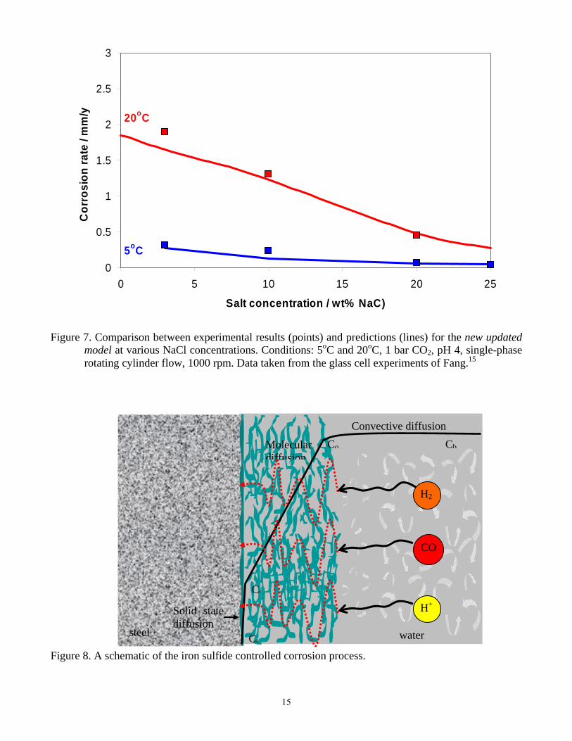
The effect of high salinity Another situation often seen in the field and rarely studied in the lab is the CO2 corrosion of mild steel in high salinity brines (>>1% by weight). Contradicting anecdotal evidence exists about the effect of very high chloride content, some suggesting that it is detrimental to survival of mild steel in CO2 saturated solutions, others suggesting that it is beneficial. This confusion carried over into the models. The original model therefore did not include any effect of high salinity. In his thesis work, Fang15 has looked at this effect as well, and found that the CO2 corrosion rates of mild steel are severely retarded with high salt concentrations across the whole temperature range. It is seen in Figure 5 that the original mechanistic model, which work reasonably well up to 3% NaCl in solution, deviates progressively as the concentration of salt increases. Higher salt concentration changes the brine physico-chemical properties comprehensively. The density and viscosity are increased; however this effect is well understood and readily modeled. As the salt concentration increases well beyond a few percent, the brine becomes a non-ideal solution. This is also well understood and can be accounted for by using a water chemistry model based on Pitzer’s theory to calculate the activity coefficients and adjust the concentrations of the various ionic species in solution. The result is shown in Figure 6, where it is seen that high salt concentration affects mainly the activity coefficient of H+ ions in saturated CO2 solutions. Consequently, the pH of a brine changes significantly with increasing salt concentration. Furthermore, high salt concentration will decrease the solubility of CO2 in the corrosion solution, another effect that is well known and readily modeled. However, even when all these effects are taken into account, the original model could not capture the effect of high salinity on diminishing uniform CO2 corrosion rate, as seen in Figure 5. By conducting a detailed electrochemical analysis, Fang15 has discovered that many other processes underlying CO2 corrosion are affected by salt concentration. The homogenous chemical reactions were predominantly influenced by the abovementioned change in activity coefficients and the decrease in the solubility of CO2 in water. The heterogeneous electrochemical reactions at the steel surface were affected in the first place by competitive adsorption and surface reaction retardation. Mass transfer coefficients were also changed for reasons beyond those related to the increased density and viscosity of the brine. When all these effects were accounted for by using the appropriate theories where available,15

and introduced into the new updated model, a much improved fit with the experimental results is obtained across the whole temperature and salinity range (Figure 7).

6

The effect of H2S Internal CO2 corrosion of mild steel in the presence of hydrogen sulfide (H2S) represents a significant problem for the oil and gas industry16-22. In CO2/H2S corrosion of mild steel, both iron carbonate and iron sulfide layers can form on the steel surface. Studies have demonstrated that surface layer formation is one of the important factors governing the corrosion rate in H2S corrosion. Until recently there were no predictive models of H2S corrosion of mild steel. Only a very rudimentary model of CO2 retardation by traces of H2S was built into the original model. In a recent study Sun24 has proposed a rather simple mechanistic model which is described below. The corrosion of mild steel in H2S aqueous environments proceeds initially by a very fast direct heterogeneous chemical reaction at the steel surface to form a solid adherent mackinawite layer. The overall reaction scheme can be written as:

( ) ( ) 22 HsFeSSHsFe +⇒+ (7) As both the initial and final state of Fe is solid, this reaction is often referred to as the “solid state corrosion reaction”. This film is very thin (<<1μm) but dense and acts as a solid state diffusion barrier for the sulfide species involved in the corrosion reaction. The thin mackinawite film continuously goes through a cyclic process of growth, cracking and delamination, what generates the outer sulfide layer which thickens over time (typically >1μm) and also presents a diffusion barrier; this outer sulfide layer is very porous and rather loosely attached, over time it may crack, peel and spall, a process aggravated by the flow. Iron sulfide precipitation and transformation may occur in long exposures and effect not accounted for in the present model. Due to the presence of the thin inner mackinawite film and the outer sulfide layer, it is assumed that the corrosion rate of steel in H2S solutions is always under mass transfer control. Based on the discussions above, a schematic of the H2S corrosion process is shown in Figure 8. According to the depiction shown one can write the flux of hydrogen sulfide due to: convective diffusion through the mass transfer boundary layer:

( )SHoSHbSHmSH cckFlux2222 ,,, −= (8)

molecular diffusion through the liquid in the porous outer layer:

( )2

2 2 2, ,H S

H S o H S i H Sos

DFlux c c

εδ

Ψ= − (9)

solid state diffusion through the inner mackinawite film:

⎟⎟⎠

⎞⎜⎜⎝

⎛=

−

SH,s

SH,iRT

B

SHSH cc

lneAFlux k

SH

2

2

2

22 (10)

where:

SHFlux2

flux of H2S expressed in mol/(m2s),

SHmk2, is the mass transfer coefficient for H2S in the hydrodynamic boundary layer,

4100012

−×= .k SH,m in nearly stagnant condition, in m/s,

7

SHbc2, is the bulk concentration of H2S in the liquid phase in mol/m3,

SHoc2, is the interfacial concentration of H2S at the outer layer/solution interface in mol/m3,

2H SD is the diffusion coefficient for dissolved H2S in water, 91000.22

−×=SHD , in m2/s, ε is the outer mackinawite layer porosity, Ψ is the outer mackinawite layer tortuosity factor,

2,i H Sc is the interfacial concentration of H2S at the inner layer/film interface in mol/m3.

osδ is the thickness of the mackinawite layer ( )/os os FeSm Aδ ρ= in m,

osm is the mass of the mackinawite layer in kg, A is the surface area of the steel in m2,

SHA2

, SHB2

are the constants in the Arrhenius equation,

2

52.0 10H SA −= × mol/(m2s) and 2

15,500H SB = J/mol,

kT is the temperature in K,

SHsc2, is the “near-zero” concentration of H2S on the steel surface and is set to 71000.1 −× in

mol/m3. In the new updated model the fluxes through the liquid boundary layer (8) and the outer sulfide scale (9) are already accounted for by the general transport equation (1). The solid state diffusion flux through the very thin mackinawite film (10) was implemented as a boundary condition on the steel surface side of the computational domain and replaces the electrochemical boundary condition (5). The prediction for

2H SFlux depends on a number of constants used in the model which can be either found in handbooks, calculated from the established theory or are determined from the experiments. The unknown thickness of the outer sulfide layer changes with time and was calculated as described below. It is assumed that the quantity of the sulfide layer retained on the metal surface at any point in time depends on the balance of:

• layer formation kinetics (as the layer is generated by spalling of the thin mackinawite film underneath it and by precipitation from the solution), and

• layer damage kinetics (as the layer is damaged by intrinsic or hydrodynamic stresses and/or by chemical dissolution)

sulfide layer sulfide layer sulfide layerretention formation damage

rate rate rate

SRR SFR SDR= − (11)

where all the terms are expressed in mol/(m2s). It is here assumed that in the typical range of application (4<pH<7), precipitation and dissolution of iron sulfide layer do not play a significant role, so it can be written:

2

2sulfide layer sulfide layerH S corrosionretention mechanicalraterate damage rate

H S mSRR CR SDR= − (12)

Where CRH2S is the corrosion rate measured in mol/(m2s). The implicit assumption is that all the corroded iron from the steel ends up as solid iron sulfide, which may adhere to or spall from the steel surface. Experiments have shown that even in stagnant conditions about half of the sulfide layer that forms is lost

8

from the steel surface due to intrinsic growth stresses by internal cracking and spalling, i.e. 0.5mSDR CR≈ . More experimentation is required to determine how the mechanical layer damage is

affected by hydrodynamic forces. Once the layer retention rate SRR is known, the change in mass of the outer sulfide layer can be easily calculated as:

os FeSm SRR M A tΔ = Δ (13) where FeSM is the molar mass of iron sulfide in kg/mol, tΔ is the time interval in seconds. The porosity of the outer mackinawite layer was determined experimentally to be very high ( 0.9ε ≈ ), however due to its layered structure the tortuosity factor was found (by trial and error) to be very low ( 0.003Ψ = ). Similar equations were derived by Sun24 for diffusion of CO2, H+ and organic acids through the sulfide layers, thus completing the model of mixed H2S /CO2 /organic acid corrosion. This model was implemented into the new updated model and extensively verified showing a remarkable agreement with the various experimental results in which the partial pressure of H2S varied from a fraction of a mbar to 10 bar. Over this large range the predictions were never more than a factor 2 different from the measured values. A sample of the comparison is shown in Figure 9 for a case of CO2 corrosion with traces of H2S, i.e. at extremely low H2S partial pressures ranging from 0.0013 – 0.32 mbar (experiments conducted by Lee23). This corresponds to 1 – 250 ppmm (by mass) in the gas phase at 1 bar CO2 and is a CO2 dominated corrosion scenario (pCO2/pH2S ratio is in the range 103 – 106). However the H2S controls the corrosion rate even when present in such minute amounts. The pure CO2 (H2S-free) corrosion rate is reduced by 3 to 10 times, due to traces of H2S, because of the formation of a mackinawite film. The model successfully captures this effect as shown in Figure 9. At the other extreme, corrosion experiments at very high temperature (120oC), high partial pressures of CO2 (pCO2=6.9 bar) and H2S (pH2S=1.38 – 4.14 bar) were recently reported by Kvarekval et al.25 In exposure lasting up to 16 days, a steadily decreasing corrosion rate was observed due to buildup of a protective iron sulfide layer. The effect of various H2S concentrations on the corrosion rate was very small. This effect was readily captured by the model with very good accuracy as seen in Figure 10. This is a situation where the H2S is the dominant corrosive species. At the highest pCO2/pH2S ratio of 5 (pCO2=6.9 bar, pH2S=1.38 bar) H2S generated approximately 70% of the corrosion rate. At the lowest pCO2/pH2S ratio of 1.67 (pCO2=6.9 bar, pH2S=4.14 bar) H2S generated 82% of the overall corrosion rate.

CONCLUSIONS New advances have been made in modelling the internal corrosion of steel pipelines which are based on the latest experimental results. The biggest advances are:

• CO2 corrosion at very low temperatures (as low as 1oC), where the corrosion rates are greatly reduced;

• CO2 corrosion in very high salinity brines (up to 25%wt. NaCl), where strong retardation of corrosion rates is seen;

• CO2 corrosion in the presence H2S where the corrosion rate is governed by formation of a iron sulfide layer by solid state reaction.

The overall model has been extensively calibrated and verified with a reliable experimental database and very good agreement was found.

9

ACKNOWLEDGEMENT The authors would like to acknowledge the contribution of the consortium of companies whose continuous financial support and technical guidance led to the publishing of this work. They are BP, ConocoPhillips, ENI, ExxonMobil, Saudi Aramco, Shell, Total, Champion Technologies, Clariant, MI Technologies and Nalco.

REFERENCES 1. C. de Waard and D.E. Milliams, Corrosion, 31 (1975): p131. 2. R. Nyborg: “Overview of CO2 Corrosion Models for Wells and Pipelines”, CORROSION/2002,

paper no. 233 (Houston, TX: NACE International, 2002). 3. S. Nesic, S. Wang, J. Cai and Y.Xiao, “Integrated CO2 Corrosion – Multiphase Flow Model”, NACE

2004, Paper No.04626, pp. 1-25, 2004. 4. S. Nesic, J. Cai, K. J. Lee, “A Multiphase Flow and Internal Corrosion Prediction Model For Mild

Steel Pipelines”, CORROSION/2005, Paper No. 556, (Houston, TX: NACE International, 2005). 5. Hernandez, S., Nesic, S., Weckman, G. and Ghai, V., “Use of Artificial Neural Networks for

Predicting Crude Oil Effect on CO2 Corrosion of Carbon Steels”, NACE 2005, Paper No.05554, 2005.

6. Y. Xiao and S. Nesic, “A Stochastic Prediction Model of Localized CO2 Corrosion”, NACE 2005, Paper No.05057, 2005.

7. J. Lee and S. Nesic “The Effect of Trace Amounts of H2S on CO2 Corrosion Investigated by Using the EIS Technique”, NACE 2005, Paper No.05630, 2005.

8. M. Nordsveen, S. Nesic, R. Nyborg and A. Stangeland, “A Mechanistic Model for Carbon Dioxide Corrosion of Mild Steel in the Presence of Protective Iron Carbonate Films - Part1: Theory and Verification”, Corrosion, Vol. 59, (2003): p. 443.

9. S. Nesic, M. Nordsveen, R. Nyborg and A. Stangeland, "A Mechanistic Model for CO2 Corrosion of Mild Steel in the Presence of Protective Iron Carbonate Films - Part II: A Numerical Experiment", Corrosion, Vol. 59, (2003): p. 489.

10. S. Nesic, K.-L.J.Lee, "A Mechanistic Model for CO2 Corrosion of Mild Steel in the Presence of Protective Iron Carbonate Films - Part Ш: Film Growth Model", Corrosion, Vol. 59, (2003): p. 616.

11. J. T. Davies, Turbulence Phenomena, (Academic Press, 1972). 12. S. Nesic, J. Postlethwaite, S. Olsen, Corrosion, “An Electrochemical Model for Prediction of

Corrosion of Mild Steel in Aqueous Carbon Dioxide Solutions”, 52, (1996): p. 280. 13. S. Nesic, N. Thevenot, J.-L. Crolet, D. Drazic, “Electrochemical Properties of Iron Dissolution in the

Presence of CO2 - Basics Revisited”, CORROSION/96, paper no. 3, (Houston, TX: NACE International, 1996).

14. S. Olsen, A. M. Halvorsen, P. G. Lunde, R. Nyborg, “CO2 Corrosion Prediction Model – Basic Principles”, CORROSION/95, paper no. 551, (Houston, TX: NACE International, 1995).

15. H. Fang, “Low Temperature and High Salt Concentration Effects on General CO2 Corrosion for Carbon Steel”, MS thesis, Ohio University, 2006.

16. D. W. Shoesmith, P. Taylor, M. G. Bailey, & D. G. Owen, J. Electrochem. Soc., The formation of ferrous monosulfide polymorphs during the corrosion of iron by aqueous hydrogen sulfide at 21 oC, 125 (1980) 1007-1015.

17. D. W. Shoesmith, Formation, transformation and dissolution of phases formed on surfaces, Lash Miller Award Address, Electrochemical Society Meeting, Ottawa, Nov. 27, 1981.

18. S. N. Smith, A proposed mechanism for corrosion in slightly sour oil and gas production, Twelfth International Corrosion Congress, Houston, Texas, September 19 – 24, paper no. 385, 1993.

10

19. S. N. Smith and E. J. Wright, Prediction of minimum H2S levels required for slightly sour corrosion, Corrosion/94, Paper no. 11, NACE International, Houston, Texas, 1994.

20. S. N. Smith and J. L. Pacheco, Prediction of corrosion in slightly sour environments, Corrosion/2002, paper no. 02241, NACE International, Houston, Texas, 2002.

21. S. N. Smith and M. Joosten, Corrosion of carbon steel by H2S in CO2 containing oilfield environments, Corrosion/2006, Paper no. 06115, NACE International, Houston, Texas, 2006.

22. M. Bonis, M. Girgis, K. Goerz, and R. MacDonald, Weight loss corrosion with H2S: using past operations for designing future facilities, Corrosion/2006, paper no. 06122, NACE International, Houston, Texas, 2006.

23. K. J. Lee, A mechanistic modeling of CO2 corrosion of mild steel in the presence of H2S, PhD dissertation, Ohio University, 2004.

24. W. Sun, Kinetic of iron carbonate and iron sulfide layer formation in CO2/H2S corrosion, PhD dissertation, Ohio University, 2006.

25. J. Kvarekval and R. Nyborg, Formation of multilayer iron sulfide films during high temperature CO2/H2S corrosion of carbon steel, paper no. 03339, NACE International, Houston, Texas, 2003.

11

0

2

4

6

8

10

0 20 40 60 80 100

Temperature / oC

Cor

rosi

on ra

te /

mm

/ypH4

pH5

pH6

Figure 1. Comparison between experimental results (points) and predictions (line) for the original

model. Conditions: 1 bar CO2, 1% NaCl solution, single-phase flow, v=1 m/s, in a 15 ID pipe. Data taken from the flow loop experiments of Nesic et al.3

0

0.5

1

1.5

2

0 2000 4000 6000 8000Velocity / rpm

Cor

rosi

on ra

te /

mm

/y

5oC1oC

5oC 1oC

Figure 2. Comparison between experimental results (points) and predictions (line) for the original model

at low temperature. Conditions: 1 bar CO2, 3% NaCl solution, pH 4, single-phase rotating cylinder flow. Data taken from the glass cell experiments of Fang.15

12

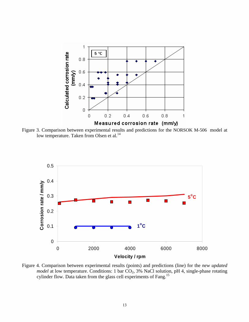
Figure 3. Comparison between experimental results and predictions for the NORSOK M-506 model at

low temperature. Taken from Olsen et al.14

0

0.1

0.2

0.3

0.4

0.5

0 2000 4000 6000 8000Velocity / rpm

Cor

rosi

on ra

te /

mm

/y

5oC

1oC

Figure 4. Comparison between experimental results (points) and predictions (line) for the new updated

model at low temperature. Conditions: 1 bar CO2, 3% NaCl solution, pH 4, single-phase rotating cylinder flow. Data taken from the glass cell experiments of Fang.15

13

0

0.5

1

1.5

2

2.5

3

0 5 10 15 20 25

Salt concentration / wt% NaC)

Cor

rosi

on ra

te /

mm

/y

5oC

20oC

Figure 5. Comparison between experimental results (points) and predictions (lines) for the original

model at various NaCl concentrations. Conditions: 5oC and 20oC, 1 bar CO2, pH 4, single-phase rotating cylinder flow, 1000 rpm. Data taken from the glass cell experiments of Fang.15

0.0

0.5

1.0

1.5

2.0

2.5

3.0

3.5

0 5 10 15 20 25 30Salt Concentration / (wt% NaCl)

Act

ivity

Coe

ffici

ent

Na+Cl-H+OH-HCO3-CO3

Figure 6. Calculated activity coefficient change with salt concentration at 20ºC at 1 bar total pressure.

14

0

0.5

1

1.5

2

2.5

3

0 5 10 15 20 25

Salt concentration / wt% NaC)

Cor

rosi

on ra

te /

mm

/y

5oC

20oC

Figure 7. Comparison between experimental results (points) and predictions (lines) for the new updated

model at various NaCl concentrations. Conditions: 5oC and 20oC, 1 bar CO2, pH 4, single-phase rotating cylinder flow, 1000 rpm. Data taken from the glass cell experiments of Fang.15

Figure 8. A schematic of the iron sulfide controlled corrosion process.

water

steel

H+

CbCo

Ci

Cs

Solid state diffusion

Molecular diffusion

Convective diffusion

CO

H2S

15

0

0.1

0.2

0.3

0.4

0.5

0.6

0.7

0.8

0.9

1

0 50 100 150 200

H2S / ppm

Cor

rosi

on ra

te /

mm

/yr

Figure 9. Corrosion rate vs. partial pressure of H2S; experimental (points), predictions using new

updated model (lines); conditions: total pressure p=1 bar, CO2 partial pressure 0.1 bar, H2S gas partial pressure from 0.0013 – 0.32 mbar, T=20oC, reaction time 24 hours, pH 5, 1000 rpm. Data taken form Lee 23.

0.1

1

10

100

0 10 20 30 40 50 60 70

pH2S / pCO2 ratio in %

Cor

rosi

on ra

te /

mm

/yr

Figure 10. Corrosion rate vs. pH2S/pCO2 ratio; experimental (points), predictions using the new updated

model (lines); conditions: total pressure p=7 bar, CO2 partial pressure 6.9 bar, H2S gas partial pressure from 1.38 – 4.14 bar, T=120oC, experiment duration up to 16 days, pH 3.95 – 4.96, liquid velocity 10 m/s. Experimental data taken from Kvarekval et al25.

16