The Visual Computer manuscript No.(will be inserted by the editor)

Idan Shatz · Ayellet Tal · George Leifman

Paper Craft Models from Meshes

the date of receipt and acceptance should be inserted later

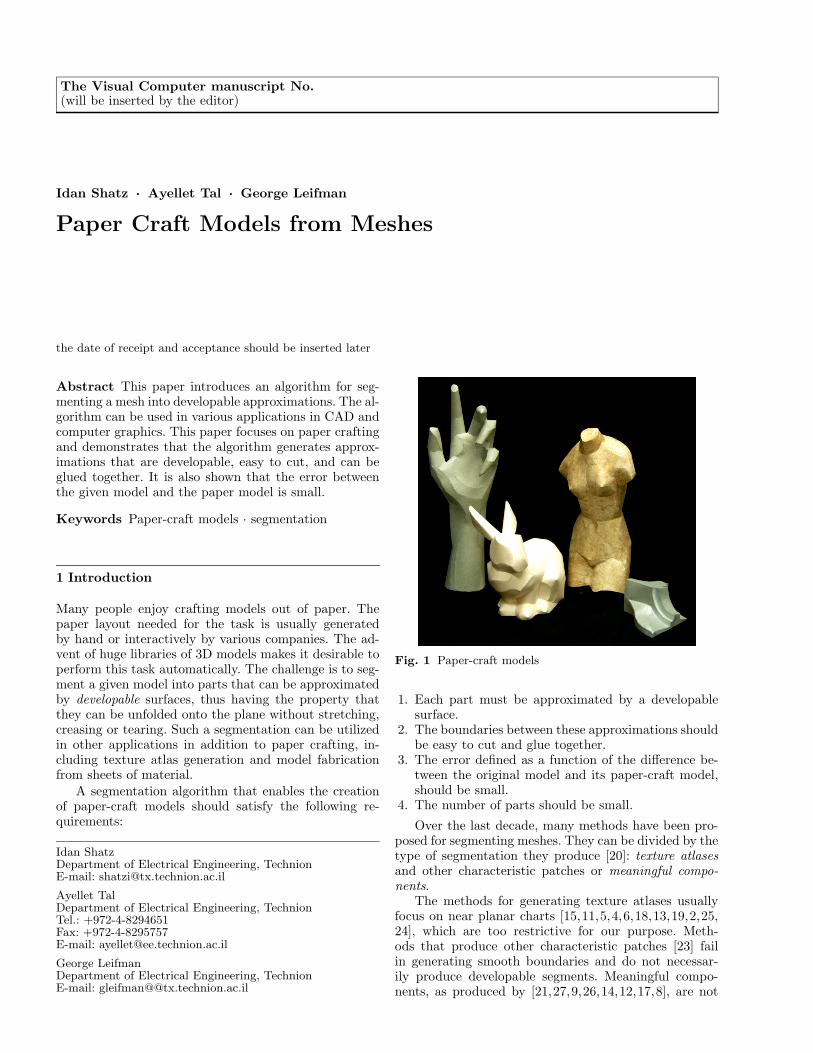
Abstract This paper introduces an algorithm for seg-menting a mesh into developable approximations. The al-gorithm can be used in various applications in CAD andcomputer graphics. This paper focuses on paper craftingand demonstrates that the algorithm generates approx-imations that are developable, easy to cut, and can beglued together. It is also shown that the error betweenthe given model and the paper model is small.

Keywords Paper-craft models · segmentation

1 Introduction

Many people enjoy crafting models out of paper. Thepaper layout needed for the task is usually generatedby hand or interactively by various companies. The ad-vent of huge libraries of 3D models makes it desirable toperform this task automatically. The challenge is to seg-ment a given model into parts that can be approximatedby developable surfaces, thus having the property thatthey can be unfolded onto the plane without stretching,creasing or tearing. Such a segmentation can be utilizedin other applications in addition to paper crafting, in-cluding texture atlas generation and model fabricationfrom sheets of material.

A segmentation algorithm that enables the creationof paper-craft models should satisfy the following re-quirements:

Idan ShatzDepartment of Electrical Engineering, TechnionE-mail: shatzi@tx.technion.ac.il

Ayellet TalDepartment of Electrical Engineering, TechnionTel.: +972-4-8294651Fax: +972-4-8295757E-mail: ayellet@ee.technion.ac.il

George LeifmanDepartment of Electrical Engineering, TechnionE-mail: gleifman@@tx.technion.ac.il

Fig. 1 Paper-craft models

1. Each part must be approximated by a developablesurface.

2. The boundaries between these approximations shouldbe easy to cut and glue together.

3. The error defined as a function of the difference be-tween the original model and its paper-craft model,should be small.

4. The number of parts should be small.

Over the last decade, many methods have been pro-posed for segmenting meshes. They can be divided by thetype of segmentation they produce [20]: texture atlasesand other characteristic patches or meaningful compo-nents.

The methods for generating texture atlases usuallyfocus on near planar charts [15,11,5,4,6,18,13,19,2,25,24], which are too restrictive for our purpose. Meth-ods that produce other characteristic patches [23] failin generating smooth boundaries and do not necessar-ily produce developable segments. Meaningful compo-nents, as produced by [21,27,9,26,14,12,17,8], are not

2 Idan Shatz et al.

developable, and thus cannot be used for paper-crafting.These general approaches are thus insufficient for ourproblem.

In the seminal paper of [16], a method is proposedfor producing strip-based approximation segmentationof meshes. This method manages to generate very prettypaper-craft models. However, strip-based approximationscreate long and jagged boundaries that can be difficultto cut and glue, contradicting Requirement 2. In [7],an algorithm for mesh segmentation into nearly devel-opable meshes is introduced and used for creating clothobjects. However, in cloth, differently from paper, thestretch factor tolerates both non-developable segmentsand non-exact boundaries. Thus, Requirements 1 and 2are less critical. Moreover, in cloth, many of the detailsof the objects are lost, and therefore Requirement 3 isoften violated.

The current paper presents a novel algorithm for seg-menting a given mesh into explicitly developable partsthat can be easily cut and glued together, satisfyingRequirements 1–4. The algorithm has three key ideas.First, each segment is approximated by a surface thatis guaranteed to be developable. Second, the approxima-tions are modified so as to guarantee that neighboringapproximations intersect at their boundaries, thus pro-hibiting stretching. Third, the algorithm extracts the an-alytical boundaries between the approximations, makingthe boundaries intuitive and easy to cut and glue. Thesegmentations produced by the algorithm were used tocreate several paper-craft models, as illustrated in Fig-ure 1.

The rest of the paper is structured as follows. Sec-tion 2 outlines the algorithm. Sections 3–5 elaborate onseveral stages of the algorithm. Section 6 displays results.Section 7 summarizes the paper.

2 Algorithm Overview

Setup: The aim of the algorithm is to segment a meshinto a small number of segments that can be well ap-proximated by developable surfaces, whose boundariescan be easily cut and glued.

A surface is developable if it has a zero Gaussian cur-vature at all points. Since this definition does not providea practical algorithm for generating a segmentation, ouralgorithm uses two types of surfaces known to be devel-opable: a planar surface and a conic surface, following [7].Our general scheme, however, can incorporate other pre-defined types of developable surfaces.

A planar surface is defined by a normal vector n anda constant d, by

< n, x >= d. (1)

There are several ways to define a conic. We define itas follows: Let c be the center of the cone base, n be thecone axis, d be the distance of a point x from the cone,

θ be a constant angle between the cone normals and thecone axis, rx be the normalized projection of x on thecone base in the axis direction, and nx be the normal ofthe cone at x. Then, a conic (n, c, d, θ) is defined by:

< nx, x − c >= d, (2)

where rx and nx are defined as follows:

rx =(x − c)− < (x − c), n > n

||(x − c)− < (x − c), n > n||,

nx = rx · sin θ + n · cos θ.

Note that a planar surface is a special case of a conic,where a conic (n, 0, d, 0) is a plane (n, d). We distinguishbetween these two types of surfaces because a plane iseasier to approximate.

Definition 1 A Segment Si of a mesh S is a connectedsub-mesh Si ⊆ S.

Definition 2 A Segment approximation: Given asegment Si ⊆ S, its approximation Ei is a conic (/plane)associated with Si.

Given a mesh, the algorithm segments it into disjointsegments S1, S2, · · ·SK whose union gives S, such thateach segment Si is approximated by Ei. The distancebetween a mesh vertex v and an approximation Ei, isdefined as the distance between the vertex and its pro-jection along its nv direction. (If v is not on Ei, nv is thedirection of the normal of the closest point on Ei.)

Distance(v,Ei) = ||v − ProjEi(v)||. (3)

The total squared error associated with a mesh andits paper-craft model is defined as the sum of distancesfrom a vertex to the approximations it is associated with,over all vertices:

Error(mesh, papermodel) =K∑

i=1

∑

v∈Si

(Distance(v,Ei))2.(4)

Algorithm: The algorithm begins with an initial over-segmentation of the mesh into trivial developable seg-ments. This initial segmentation is iteratively modified,by decreasing the number of segments, while increas-ing the error (Equation 4). Each such iteration approx-imates the current segments, by fitting each segment toa conic(/plane), using weights specific to our problem.

Once the segmentation is determined, the approxima-tions are modified, in order to accommodate for “good”boundaries. Then, the analytical boundaries between theapproximations are computed, therefore not restrictingthe boundaries to pass through edges of the originalmesh. The five stages of the algorithm are briefly de-scribed below and explained in detail in the subsequentsections.

Paper Craft Models from Meshes 3

1. Computation of an initial segmentation: Initially, aplanar surface is associated with every face of themesh, making it a trivial segmentation into devel-opable segments with zero error. Then, neighboringsegments are merged if the error (Equation 4) is smallerthan a pre-defined error. At the end of this stage, themodel is over segmented with a very small error.

2. Iterative segmentation modification: The initial seg-mentation is iteratively modified by applying two op-erations successively. First, neighboring segments aremerged, thus decreasing the total number of segments.Second, the fit between each new segment and itsconic approximation is optimized. While the first op-eration increases the error, the second decreases it. Ineach iteration, the total error is allowed to increase,until either a pre-defined error or a pre-defined num-ber of segments is reached. This stage is described indetail in Section 3.

3. Boundary refinement: The previous stage approxi-mated each segment by a conic (/plane) indepen-dently. As a result, neighboring approximations mightnot intersect each other, or might intersect each otherat boundaries that are far from the boundaries be-tween their corresponding segments. The current stageof the algorithm modifies the approximations, so asto take the boundaries into account, as discussed inSection 4.

4. Extraction of analytical boundaries: At this stage, theanalytical boundaries between the conic approxima-tions are computed. These boundaries are importantfor two reasons. First, conic edges are easy to cut-and-glue, in contrary to jagged mesh boundaries. Sec-ond, analytical boundaries guarantee that neighbor-ing conics meet, which is a vital requirement in paper-crafting (Requirement 2). This stage is discussed inSection 5.

5. Segment drawing: After finding the analytical bound-aries between segments, they are projected to theplane and printed, adding cuts to conic rings.

Pre-processing: The algorithm described above can beapplied to the full mesh. However, two pre-processingsteps improve the results. First, a symmetry plane ofthe model is found, when it exists. The algorithm is ap-plied to half of the model, and the result of the segmen-tation is duplicated. Second, an existing segmentationinto meaningful components (e.g., [9]) is used and thealgorithm is applied to each component separately. Bothpre-processing steps make paper-crafting more intuitive,since users prefer to work on “semantically meaningful”components, such as the “left and right arm, the “‘leftand right leg” etc.

The symmetry plane is determined by finding theprincipal axes of the mesh. There are two types of sym-metry: rotation and reflection. Any axis of a rotationsymmetry through the origin, as well as the normal ofthe reflection symmetry plane through the origin, is aprincipal axis [10]. The algorithm first finds the princi-

pal axes of the model using PCA. The Hausdorff distancebetween the reflected sets of points on both sides of thereflection plane is then used to evaluate the accuracyof reflection symmetry plane. If the distance is smallerthan a threshold, the plane is used as a symmetry plane.Otherwise, the algorithm is applied without symmetry.

The following sections elaborate on Steps 2, 3 and 4.

3 Iterative segmentation modification

This stage (Stage 2) applies an iterative region growingapproach, using a variant of the K-means algorithm [3].Every iteration of the algorithm performs the followingoperations:

1. The faces of the mesh are re-distributed into the cur-rent segments. This is done by assigning each faceto the conic approximation that best fits it. (In thefirst iteration, the approximations found in Stage 1are used.)The error associated with a face is defined as a func-tion of its distance from the approximation and thedistance of the normals.

2. Each segment is re-approximated by a plane or aconic, using a standard non-linear squared optimiza-tion procedure [22].Then, the algorithm goes back to Step 1, until eithera pre-set number of iterations (10) is reached or untilthe error does not change from the previous iteration.In this case, the algorithm proceeds to Step 3.

3. Neighboring segments are merged and approximated,until the current error bound is reached.The error bound is increased and the algorithm goesback to Step 1.

Below, we elaborate on each of these operations.

Step 1: A face is assigned to a segment if the averagedistance between its vertices and the segment’s approxi-mation is small. The distance depends both on the pro-jection distance (Equation 3) and on the match betweenthe face normals and the approximation, which was em-pirically found to be important. Specifically, let Ei bethe approximation of a given segment Si and f be theface whose distance to Ei we wish to compute. Then,

dist(f,Ei) = NormDiff(f,Ei) ·∑

v∈f

Distance(v,Ei),(5)

NormDiff(f,Ei) = 1+λ∑

v∈f

(1 − | < NEi(v), N(f) > |),

where NEi(v) is the normal of Ei at the projection of v

on Ei, N(f) is the normal of f , and λ is a user-definedparameter. This step is performed in a Breadth-FirstSearch (BFS) manner, thus guaranteeing connectivity.

4 Idan Shatz et al.

Step 2: Given a set of vertices associated with normals,the optimization function attempts to fit both the bestconic and the best plane to this set. The surface havingthe smaller error is chosen. Each face f is assigned aweight ω(f), which is the normalized area of the face.The area “hints” to the importance of the face vertices.The function optimized in this step is given by:

argminn,d,c,θ

∑

f

(ω(f)Dist(f,E(n, d, c, θ)))2 (6)

Step 3: To decrease the number of segments, neighboringsegments are merged. The segments selected for mergingare those whose merge causes the smallest projection er-ror (Equation 4).

4 Boundary refinement

When two segments intersect in a boundary along edgesof the mesh, there should be an analytical boundary be-tween their approximations, close to the boundary edges.However, as the error between an approximation and itscorresponding segment grows, it might not be satisfied,as illustrated in Figure 2. It is clear that approximatingeach segment separately cannot suffice.

Fig. 2 The problem with boundaries

The challenge is to bring the analytical boundary be-tween adjacent approximations as close as possible to theboundary between their corresponding segments. This isdone by considering the boundaries in the optimizationprocess. The distance between the projections of bound-ary vertices on the adjacent approximations, is added toEquation 6 and each approximation Ei is optimized by:

argminn,d,c,θ

∑

f∈Ei

(ω(f) · Dist(f,E(n, d, c, θ)))2

+β∑

u∈boundary

(ω(u)ProjError(u))2. (7)

In Equation 7, u is a boundary vertex adjacent to Seg-ments Si and Sk. Denote the projection of u on Ei (Ek)by ui (uk). We define the projection error of u by ProjError(u) =||ui−ProjEi

(uk)||. (ω(v) will be defined later.) Note that

this second term is 0 when the approximations are per-fectly aligned.

At every optimization iteration, the algorithm in-creases the value of β. (When β −→ ∞, the approxima-tions will meet, but the projection error will grow.) Thealgorithm terminates when β gives a sufficiently smallerror, so that the boundaries of the approximations areclose. In the implementation, β is initialized to 0 andincreased by 0.1 at every iteration, where convergence isreached after 10-20 iterations.

Note that this stage of the algorithm is similar to theprevious stage (Section 3). Both perform the optimiza-tion described in Equation 7, with the only differencebeing the value of β. However, it is important to per-form these two stages separately since the addition ofthe second term (β > 0) requires a stable segmentation.

“Flat boundaries”: When the boundaries of adjacent ap-proximations have similar normals, their analytical bound-ary becomes unstable. This situation, which might becounter-intuitive, is illustrated in Figure 3. The approxi-mations are drawn in yellow and green and the analyticalboundary between them in red. The blue region demon-strates how the red boundary moves when the yellow ap-proximation changes slightly. It is shown that the blueregion increases when the normals at the boundary ofthe approximations are similar.

Fig. 3 Sharp (left) vs. flat (right) boundary

To understand this behavior, assume that we are giventwo planar surfaces p1 and p2, having normals n1 andn2, respectively. Assume also that p1 moves in the direc-tion of its normal n1 by ∆d1, as illustrated in Figure 4.The movement of the boundary between p1 and p2, isdescribed by Equation 8

∆d =∆d1

‖n1 × n2‖. (8)

A boundary is called flat when α ≈ 0◦ (‖n1 × n2‖ ≈0). It can be seen from Equation 8 that when α ≈ 0◦,a small movement of p1 (∆d1) will result in a large ∆d.Therefore, the projection error of a flat boundary vertex(∆d1) will cause a large error in the analytical boundary(∆d). To handle it, the weights ω in Equation 7 should

Paper Craft Models from Meshes 5

Fig. 4 p1 moves by ∆d1 in direction n1

depend on ∆d. In our implementation, the weight of aboundary vertex u is set to

ω(u) =1

‖n1 × n2‖ + ε.

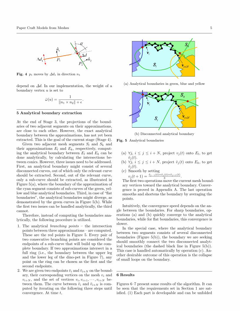
5 Analytical boundary extraction

At the end of Stage 3, the projections of the bound-aries of two adjacent segments on their approximations,are close to each other. However, the exact analyticalboundary between the approximations, has not yet beenextracted. This is the goal of the current stage (Stage 4).

Given two adjacent mesh segments Sl and Sk andtheir approximations El and Ek, respectively, comput-ing the analytical boundary between El and Ek can bedone analytically, by calculating the intersections be-tween conics. However, three issues need to be addressed.First, an analytical boundary might consist of severaldisconnected curves, out of which only the relevant curveshould be extracted. Second, out of the relevant curve,only a sub-curve should be extracted, as illustrated inFigure 5(a), where the boundary of the approximation ofthe cyan segment consists of sub-curves of the green, yel-low and blue analytical boundaries. Third, in case of “flatboundaries”, the analytical boundaries might diverge, asdemonstrated by the green curves in Figure 5(b). Whilethe first two issues can be handled analytically, the thirdcannot.

Therefore, instead of computing the boundaries ana-lytically, the following procedure is utilized.

1. The analytical branching points – the intersectionpoints between three approximations – are computed.These are the red points in Figure 5. Every pair oftwo consecutive branching points are considered theendpoints of a sub-curve that will build up the com-plete boundary. If two approximations intersect in afull ring (i.e., the boundary between the upper legand the lower leg of the dino-pet in Figure 7), anypoint on the ring can be chosen as the first and thesecond endpoints.

2. We are given two endpoints vi and vi+N on the bound-ary, their corresponding vertices on the mesh vi andvi+N , and the set of vertices vi, vi+1, · · · , vi+N be-tween them. The curve between vi and vi+N is com-puted by iterating on the following three steps untilconvergence. At time t,

(a) Analytical boundaries in green, blue and yellow

(b) Disconnected analytical boundary

Fig. 5 Analytical boundaries

(a) ∀j, i ≤ j ≤ i + N, project vj(t) onto El, to getvj(t).

(b) ∀j, i ≤ j ≤ i + N, project vj(t) onto Ek, to getvj(t).

(c) Smooth by setting

vj(t + 1) =vj−1(t)+vj(t)+vj+1(t)

3 .The first two operations move the current mesh bound-ary vertices toward the analytical boundary. Conver-gence is proved in Appendix A. The last operationsmooths and shortens the boundary by averaging thepoints.

Intuitively, the convergence speed depends on the an-gle between the boundaries. For sharp boundaries, op-erations (a) and (b) quickly converge to the analyticalboundaries, while for flat boundaries, this convergence isslower.

In the special case, where the analytical boundarybetween two segments consists of several disconnectedboundaries (Figure 5(b)), the boundary we are seekingshould smoothly connect the two disconnected analyt-ical boundaries (the dashed black line in Figure 5(b)).This case is handled automatically by operation (c). An-other desirable outcome of this operation is the collapseof small loops on the boundary.

6 Results

Figures 6–7 present some results of the algorithm. It canbe seen that the requirements set in Section 1 are sat-isfied. (1) Each part is developable and can be unfolded

6 Idan Shatz et al.

(a) original model (b) paper-craft model (c) part layout

Fig. 6 Paper-craft models of Venus (700 faces), a CAD model (11K faces) , and a hand (25K faces)

Paper Craft Models from Meshes 7

(a) original model (b) paper-craft model (c) part layout

Fig. 7 Paper-craft models of the dino-pet (3.5K faces) and the duck (1100 faces)

(a) Our algorithm (b) [Mitani & Suzuki] (c)[Julius et al]

Fig. 8 Comparison

8 Idan Shatz et al.

into a paper (Figures 6–7(c)). (2) The boundaries goalong piece-wise conic edges and are easy to cut andglue. (3) Visually, the difference between the paper-craftmodel and the mesh is pretty small. Below we presentthe measured error. (4) The number of pieces is relativelysmall.

In Figure 6, no pre-processing was applied to themodels, while in Figure 7, both symmetry and segmen-tation into meaningful components were used in a pre-processing stage. (However, the algorithm identified thecylindrical features of meshes, such as the legs, hands,and neck even without pre-processing.)

In terms of accuracy, our algorithm has the advantagethat the error can be bounded, by setting the maximumerror in Stages 1 and 2 of the algorithm. In particular,the maximum error was set to 0.05 (for all the models),normalized by the size of the model.

Figure 8 compares the results of our algorithm tothose of [16] and [7]. It can be seen that in [7] many ofthe details disappear, including the front legs, the tailand the protrusion of the rear leg. It can be concludedthat the error is large (though it is not supplied). In [16],the paper-craft model presents the details. In this case,the error can be compared numerically. The RMS (rootmean square) error measured by Metro [1] between theoriginal model and the paper-craft model (projecting thevertices onto the approximations) of the bunny is 0.0077,compared to 0.0126 reported by [16].

As for the other requirements: Cutting and gluingis easier when cones are used, rather than long trianglestrips [16]. It worth noting that other algorithms haveattempted to smooth the mesh boundaries [9,7]. How-ever, these boundaries are restricted to the edges of themesh, and thus are bound to be jagged. In our algorithm,the analytical boundaries solves jagginess.

Finally, our algorithm produces 35 parts for the bunny,while [16] produces 33 parts, thus this aspect is compa-rable. In [7], only 10 parts are produced, which is accept-able for cloth, but cannot suffice for creating an accuratemodel from paper.

Our algorithm has several other desirable properties.First, since conics are used, the paper model is rela-tively smooth. Moreover, the paper model looks smootheven when the input mesh contains very few triangles(e.g., only 912 faces in Venus in Figure 6). Second, whena part is thin (i.e., the hands of the dino-pet in Fig-ure 7), it is modeled by a single planar part. This makespaper-crafting much easier for the user. Third, it canbe observed that regions with many details have moresegmented than regions with less details. This propertyhelps reducing the number of pieces, while preserving thedetails of the model. Finally, the use of symmetry, whenit exists, makes paper crafting intuitive.

Two parameters need to be set by the user: the max-imum error allowed and λ, which specifies the weightgiven to the normals. The first parameter makes it pos-sible to generate different segmentations of different ac-

curacy for a given mesh, so that the effort is suitable forchildren at various ages. To produce the paper-craft ex-amples shown in this paper, the error was set to 5% oflargest axis of the model’s bounding box and λ was setto 5. The exception is the bunny, for which λ was set to3. Thus, almost no parameter tweaking was necessary.

For the actual gluing of the paper-craft , the gluinginstructions are printed on the reverse side of the paper.In particular, the segment number is printed within thesegment and the numbers of the neighbors are printedalong the corresponding boundaries. Theses numbers guidethe user in assembling the parts. Because of the piece-wise smooth boundaries, it is easy to understand whereeach sub-boundary begins and ends.

7 Conclusion

This paper introduces an algorithm for segmenting amesh into developable components. The algorithm hasthree key ideas. First, each segment is approximatedby a surface that is guaranteed to be developable. Sec-ond, the approximations are modified so as to guaran-tee that neighboring approximations indeed intersect attheir boundaries. This is important when making pa-per craft models, where stretching is prohibitive. Third,the algorithm extracts the analytical boundaries betweenthe approximations, making the boundaries intuitive andeasy to cut and glue.

In addition to satisfying Requirements 1-4, our al-gorithm has other benefits. First, the user can set pa-rameters that indicate the required level of difficulty.Thus, the algorithm trades-off error for the number ofpieces. Second, thin parts are modeled as planar sur-faces. Third, symmetry and meaningful components areexploited, which facilitate the understanding of the user.Fourth, the resulting models are piece-wise smooth. Fi-nally, regions with many details are allocated more piecesthan regions with fewer details.

The segmentations produced by the algorithm areused to create several paper layouts from existing 3Dmeshes. The resulting paper-craft models are presentedand compared to the results of other algorithms.

In the future, the algorithm can be extended to in-clude other developable surfaces, such as swept surfaceswith extrusion. Moreover, although the aim of our algo-rithm is paper-crafting, it might worth examining whetherthis method is suitable also for other applications, suchas texture mapping, where the developability constraintcan be relaxed and therefore the number of charts canbe reduced.

The technology described in this paper is patent pend-ing.

Paper Craft Models from Meshes 9

References

1. Cignoni, P., Rocchini, C., Scopigno, R.: Metro: measuringerror on simplified surfaces. Computer Graphics Forum17(2), 167–174 (1998)

2. Cohen-Steiner, D., Alliez, P., Desbrun, M.: Variationalshape approximation. ACM Trans. Graph. 23(3), 905–914 (2004)

3. Duda, R., Hart, P., Stork, D.: Pattern Classification.John Wiley & Sons, New York (2000)

4. Garland, M., Willmott, A., Heckbert, P.: Hierarchicalface clustering on polygonal surfaces. In: SI3D ’01: Pro-ceedings of the 2001 symposium on Interactive 3D graph-ics, pp. 49–58 (2001)

5. Guskov, I., Vidimce, K., Sweldens, W., Schroder, P.: Nor-mal meshes. In: SIGGRAPH, pp. 95–102 (2000)

6. Igarashi, T., Cosgrove, D.: Adaptive unwrapping for in-teractive texture painting. In: SI3D ’01: Proceedings ofthe 2001 symposium on Interactive 3D graphics, pp. 209–216 (2001)

7. Julius, D., Kraevoy, V., Sheffer, A.: D-charts: Quasi-developable mesh segmentation. In: Computer Graph-ics Forum, vol. 24, pp. 581–590. Eurographics, Blackwell,Dublin, Ireland (2005)

8. Katz, S., Leifman, G., Tal, A.: Mesh segmentation usingfeature point and core extraction. The Visual Computer21(8-10), 865–875 (2005)

9. Katz, S., Tal, A.: Hierarchical mesh decomposition usingfuzzy clustering and cuts. ACM Trans. Graph. (SIG-GRAPH) 22(3), 954–961 (2003)

10. Kleppner, D., Kolenkow, R.J.: An Introduction to Me-chanics. McGraw-Hill (1973)

11. Krishnamurthy, V., Levoy, M.: Fitting smooth surfaces todense polygon meshes. In: SIGGRAPH ’96: Proceedingsof the 23rd annual conference on Computer graphics andinteractive techniques, pp. 313–324 (1996)

12. Lee, Y., Lee, S., Shamir, A., Cohen-Or, D., Seidel, H.P.:Intelligent mesh scissoring using 3d snakes. In: PacificConference on Computer Graphics and Applications, pp.279–287 (2004)

13. Levy, B., Petitjean, S., Ray, N., Maillot, J.: Least squaresconformal maps for automatic texture atlas generation.In: SIGGRAPH, pp. 362–371 (2002)

14. Liu, R., Zhang, H.: Segmentation of 3d meshes throughspectral clustering. In: Pacific Conference on ComputerGraphics and Applications, pp. 298–305 (2004)

15. Maillot, J., Yahia, H., Verroust, A.: Interactive texturemapping. In: SIGGRAPH, pp. 27–34 (1993)

16. Mitani, J., Suzuki, H.: Making papercraft toys frommeshes using strip-based approximate unfolding. ACMTrans. Graph. 23(3), 259–263 (2004)

17. Mortara, M., Patane, G., Spagnuolo, M., Falcidieno, B.,Rossignac, J.: Plumber: A multi-scale decomposition of3d shapes into tubular primitives and bodies. Proc. ofSolid Modeling and Applications pp. 139–158 (2004)

18. Sander, P., Snyder, J., Gortler, S., Hoppe, H.: Texturemapping progressive meshes. In: SIGGRAPH, pp. 409–416 (2001)

19. Sander, P., Wood, Z., Gortler, S., Snyder, J., Hoppe, H.:Multi-chart geometry images. In: Eurographics/ACMSIGGRAPH symposium on Geometry processing, pp.146–155 (2003)

20. Shamir, A.: A formalization of boundary mesh segmen-tation. In: Proceedings of the second International Sym-posium on 3DPVT (2004)

21. Shlafman, S., Tal, A., Katz, S.: Metamorphosis of poly-hedral surfaces using decomposition. Computer GraphicsForum 21(3), 219–228 (2002)

22. Taubin, G.: Estimation of planar curves, surfaces, andnonplanar space curves defined by implicit equations

with applications to edge and range image segmentation.IEEE Transactions on Pattern Analysis and Machine In-telligence 13(11), 1115–1138 (1991)

23. Wu, J., Kobbelt, L.: Structure recovery via hybrid varia-tional surface approximation. Computer Graphics Forum24(3), 277–284 (2005)

24. Yamauchi, H., Gumhold, S., Zayer, R., Seidel, H.P.: Meshsegmentation driven by gaussian curvature. The VisualComputer 21(8-10), 659–668 (2005)

25. Zhou, K., Synder, J., Guo, B., Shum, H.Y.: Iso-charts:Stretch-driven mesh parameterization using spectralanalysis. In: Eurographics/ACM SIGGRAPH sympo-sium on Geometry processing, pp. 45–54 (2004)

26. Zhou, Y., Huang, Z.: Decomposing polygon meshes bymeans of critical points. In: MMM, pp. 187–195 (2004)

27. Zuckerberger, E., Tal, A., Shlafman, S.: Polyhedral sur-face decomposition with applications. Computers andGraphics 26(5), 733–743 (2002)

A Convergence of analytical boundaries

In Section 5, a three-step procedure was proposed for con-verging to the analytical boundaries. We show that the firsttwo steps, which project the mesh vertices onto the approxi-mations, indeed converge.

Given a vertex v on segments Sl and Sk, let v(t) be thevalue of the vertex found in Step 3 at iteration t − 1 andProjEl

(v(t)) = v(t) be the projection of v(t) on El. It is easyto see that the nearest point on El to v is the projection ofv onto El. We define the mutual distance of v(t) from bothapproximations by

Dist(v(t), El ∪ Ek) =

= max{Distance(v(t), El), Distance(v(t), Ek)}.

Lemma 1 The mutual distance Dist(v(t), El ∪ Ek) == Distance(v(t), El), t > 1.

Proof After the first iteration, v(t) resides on Ek, thereforeits distance from Ek is zero and the mutual distance must bethe distance from El.

Lemma 2 The mutual distance decreases with each itera-tion, i.e., Dist(v(t + 1), El ∪ Ek) < Dist(v(t), El ∪ Ek).

Proof Let nk(v) be the normal of Ek at ProjEk(v), αkl(v)

be the angle between nk(v) and nl(v), linek(v(t)) be theline from Ek’s apex to v(t), circlek(v(t)) be the cross sec-tion through v(t) that is parallel to the axis of Ek’s, andvc(t) be the intersection of linek(v(t + 1)) and circlek(v(t)).See Figure 9(a).

The distance between v(t) and line [v(t + 1), v(t)] issin(αkl(v(t)))‖v(t) − v(t)‖. Therefore,‖v(t + 1) − v(t)‖ ≥ sin(αkl(v(t)))‖v(t) − v(t)‖.

When αkl(v(t)) > 0, ‖v(t + 1) − v(t)‖ > 0. From thetriangle inequality:‖v(t) − v(t)‖ + ‖v(t) − v(t + 1)‖ ≥ ‖v(t + 1) − v(t)‖ > 0.

As a result, one of the summands must be positive. If thefirst summand is positive, ‖vc(t)− v(t)‖ < ‖v(t)− v(t)‖. Thisstems from the fact that vc(t) resides on circlek(v(t)) andon linek(v(t)) and thus vc(t) is the nearest point to v(t) oncirclek(v(t)). (Figure 9(b) illustrates the case where v(t) isexternal to the cone).

If the second summand is positive,‖v(t + 1) − v(t)‖ <‖vc(t) − v(t)‖. This stems from the fact that vc(t) is onlinek(v(t + 1)) and v(t + 1) is the projection of v(t) on Ek,and thus {v(t + 1), v(t), vc(t)} is a right triangle with a rightangle at v(t + 1). Consequently, when αkl(v(t)) > 0,

‖v(t + 1) − v(t)‖ < ‖v(t) − v(t)‖. (9)

10 Idan Shatz et al.

This fact can be used to show convergence:

Dist(v(t + 1), El ∪ Ek) =(Lemma 1) = Distance(v(t + 1), El)

= ‖v(t + 1) − Projl(v(t + 1))‖(nearest point) ≤ ‖v(t + 1) − Projl(v(t))‖(Equation 9) < ‖v(t) − Projl(v(t))‖

= Distance(v(t), El)(Lemma 1) = Dist(v(t), El ∪ Ek).

When αkl(v(t)) = 0, Ek and El are parallel. If they donot intersect, the procedure converges to the nearest pointson them.

(a) Definitions

(b) vc(t) is the nearest point to v(t) on circlek(v(t))

Fig. 9 Proof illustration