Full Terms & Conditions of access and use can be found athttp://www.tandfonline.com/action/journalInformation?journalCode=lecr20

Download by: [Laszlo Matyas] Date: 10 December 2015, At: 01:04

Econometric Reviews

ISSN: 0747-4938 (Print) 1532-4168 (Online) Journal homepage: http://www.tandfonline.com/loi/lecr20

The Estimation of Multidimensional Fixed EffectsPanel Data Models

Laszlo Balazsi , Laszlo Matyas & Tom Wansbeek

To cite this article: Laszlo Balazsi , Laszlo Matyas & Tom Wansbeek (2015): The Estimationof Multidimensional Fixed Effects Panel Data Models, Econometric Reviews, DOI:10.1080/07474938.2015.1032164

To link to this article: http://dx.doi.org/10.1080/07474938.2015.1032164

Accepted author version posted online: 07Apr 2015.Published online: 07 Apr 2015.

Submit your article to this journal

Article views: 21

View related articles

View Crossmark data

Econometric Reviews, 0(0):1–23, 2015Copyright © Taylor & Francis Group, LLCISSN: 0747-4938 print/1532-4168 onlineDOI: 10.1080/07474938.2015.1032164

The Estimation of Multidimensional Fixed Effects PanelData Models

Laszlo Balazsi1, Laszlo Matyas1, and Tom Wansbeek2

1Department of Economics, Central European University, Budapest, Hungary2University of Groningen, Groningen, The Netherlands

This article introduces the appropriate within estimators for the most frequently used three-dimensional fixed effects panel data models. It analyzes the behavior of these estimators inthe cases of no self-flow data, unbalanced data, and dynamic autoregressive models. Themain results are then generalized for higher dimensional panel data sets as well.

Keywords Dynamic panel data model; FDI; Fixed effects; Gravity models;Multidimensional panel data; Panel data; Trade models; Unbalanced panel.

JEL Classification C1; C2; C4; F17; F47.

1. INTRODUCTION

Multidimensional panel data sets are becoming more readily available and are used tostudy a variety of phenomena like the following ones: 1) international trade and/orcapital flows between countries or regions; 2) the trading volume across several productsand stores over time (three panel dimensions); and 3) the number of passengers betweenmultiple airport hubs for different airlines (four panel dimensions). Over the years several,mostly fixed effects, specifications have been worked out to take into account the specificthree (or higher) dimensional nature and heterogeneity of these kinds of data sets. Thesemodels are linear regression models differing in the specification of the fixed effects. Asin the case of the familiar two-dimensional (2D) fixed effects panel data models, theycan simply be estimated by ordinary least squares (OLS). However, the large number ofdummy variables can make this computationally difficult or even impossible which holdsa fortiori when the dimensionality of the data is three or more. This problem is usuallysolved by the within transformation and thus invoking the Frisch–Waugh theorem (see,for example, Gourieroux and Monfort, 1995, and Greene, 2012). This states that in a

Address correspondence to Laszlo Matyas, Department of Economics, Central European University,Nador u. 9, Budapest 1051, Hungary; E-mail: matyas@ceu.edu

Dow

nloa

ded

by [

Las

zlo

Mat

yas]

at 0

1:04

10

Dec

embe

r 20

15

2 L. BALAZSI ET AL.

linear regression model, using matrix notation, with a partitioned regressor set (X, D),

y = X� + D� + � (1)

the OLS estimator for � can be obtained by regressing y on X, with y = MDy, X = MDX,and MD = I − D(D

′D)−D

′, the matrix that projects into the space orthogonal to D. In our

case, D matrix contains the dummy variables corresponding to the fixed effects. When thedata set is balanced, computing y and X is a matter of some simple scalar transformations,as is well-known from the ANOVA literature (see, for example, Scheffé, 1959).

This sets the stage for our article. In Section 2, we line up various fixed effectsmodel specifications proposed in the literature for three-dimensional data. For eachof these models, we present specific D and MD matrices and derive the “tilde” scalartransformations. Often, the data are flow type, where the nature of the observationsis such that there are no self-flows. This requires different and more complicatedtransformations. To get the feeling for what is at stake, in Section 3 we analyze the two-way model, which has not yet been described in the literature, and discuss from there thevarious three-way cases. Data with no self-flow are a rather well-behaved special kind ofunbalanced data as they still allow for fairly simple scalar transformations. The situationis less favorable in the general unbalanced case, as shown in Section 4.

In Sections 2, 3, and 4, only static models were considered. In Section 5, we show howthe presence of the lagged dependent variable may render OLS on the transformed datainconsistent, thus generalizing the well-known Nickell (1981) bias. Somewhat surprisinglywith three-way data, inconsistency does not occur in all models. For the cases withinconsistency we present the appropriate generalization of the Arellano–Bond estimator.Section 6 concludes.

Throughout the article, we use the conventional ANOVA notation and indicate theaverage over an index for a variable by denoting a bar on the variable and a dot on theplace of that index. When discussing unbalanced data, a plus sign at the place of an indexindicates summation over that index. The matrix M with a subscript denotes projectionorthogonal to the space spanned by the subscript.

2. MODELS WITH DIFFERENT TYPES OF HETEROGENEITY AND THE WITHINTRANSFORMATION

In three-dimensional panel data sets, the dependent variable of a model is observedalong three indices, such as yijt, i = 1, � � � , Ni, j = 1, � � � , Nj , and t = 1, � � � , T . As ineconomic flows, such as trade, foreign direct investment (FDI), etc., there is some kindof reciprocity, we assume to start with, that Ni = Nj = N . Implicitly, we also assume thatthe set of individuals in the observation sets i and j are the same, although we relax theseassumptions later on. The main question is how to formalize the individual and timeheterogeneity—in our case, the fixed effects.

Dow

nloa

ded

by [

Las

zlo

Mat

yas]

at 0

1:04

10

Dec

embe

r 20

15

MULTIDIMENSIONAL FIXED EFFECTS MODELS 3

2.1. The Model with Three Effects

The first attempt to properly extend the standard fixed effects panel data model [see,for example, Baltagi (2005) or Balestra and Krishnakumar (2008)] to a multidimensionalsetup was proposed by Matyas (1997). The specification of this model is

yijt = �′xijt + �i + �j + �t + �ijt i = 1, � � � , N j = 1, � � � , N , t = 1, � � � , T , (2)

where the �i, �j , and �t parameters are the country and time-specific fixed effects, the xijt

variables are the usual covariates, � (K × 1) is the vector of the structural parameters;and �ijt are the i.i.d. (0, 2

�) idiosyncratic disturbance terms. We also assume that thecovariates and the disturbance terms are uncorrelated. Now, in model (1), y is the vectorof the dependent variable of size (N 2T × 1); X is the matrix of the covariates of size(N 2T × K);

D = (IN ⊗ lNT , lN ⊗ IN ⊗ lT , lN 2 ⊗ IT )

is the (N 2T × (2N + T)) dummy matrix with column rank (2N + T − 2) correspondingto the fixed effects, with IN and lN being the identity matrix and the column vector ofones, respectively, with the sizes indicated in the index; and � = (�′, �′, �′)′ is the ((2N +T) × 1) vector of the fixed effects. Wansbeek (1991) has shown that the column space ofD does not change by replacing IN (or similarly IT ) with any (GN , lN ) orthonormal matrixof order (N × (N − 1)), where GN has to satisfy the following conditions:

G′N lN = 0, and G′

N GN = IN−1 with lN ≡ lN /√

N �

As matrix D spans the same vector space as the orthonormal matrix

D ≡ ((GN ⊗ lN ⊗ lT ), (lN ⊗ GN ⊗ lT ), (lN ⊗ lN ⊗ GT ), (lN ⊗ lN ⊗ lT )

),

which has in fact full column rank (2N + T − 2), the projection matrix of size (N 2T ×N 2T) to eliminate D is simply

MD ≡ IN 2T − DD′

= IN 2T − (QN ⊗ �JNT ) − (�JN ⊗ QN ⊗ �JT ) − (�JN 2 ⊗ QT ) −�JN 2T

= IN 2T − (IN ⊗ �JNT ) − (�JN ⊗ IN ⊗ �JT ) − (�JN 2 ⊗ IT ) + 2�JN 2T ,

with �JN ≡ lN l′N = lN l′N /N and QN ≡ GN G′N = IN −�JN . This matrix operation defines the

scalar transformation

yijt = yijt − yi�� − y�j� − y��t + 2y��� (3)

Dow

nloa

ded

by [

Las

zlo

Mat

yas]

at 0

1:04

10

Dec

embe

r 20

15

4 L. BALAZSI ET AL.

Note that this optimal within transformation actually numerically gives the sameparameter estimates as the direct OLS estimation of model (2). We must emphasizethat these within transformations are usually not unique. For example, a simpletransformation that also eliminates the fixed effects from model (2) is

yijt = yijt − yij� − y��t + y��� (4)

This model is suited to deal with purely cross-sectional data as well (that is, whenT = 1). In this case, there are only the �i and �j fixed effects and the appropriate withintransformation is yijt = yij − y�j − yi� + y��.

2.2. Models with Composite Effects

There is no reason to stop at model (2) after we derive its optimal within transformation,as similar reasoning can be done for models with different fixed effects formulations. Wecollect them here with their unique D dummy matrices, D orthonormal matrices, and MD

optimal projection matrices.A model has been proposed by Egger and Pfaffermayr (2003) which takes into account

bilateral interaction effects. The model specification is

yijt = �′xijt + �ij + �ijt, (5)

where the �ij are the bilateral specific fixed effects. Now

D = (IN ⊗ IN ⊗ lT ) of size (N 2T × N 2),

D = (IN ⊗ IN ⊗ lT ) of size (N 2T × N 2),

both with full column ranks N 2. The optimal projection matrix orthogonal to D is

MD = IN 2T − (IN 2 ⊗ �JT ),

defining the scalar operation

yijt = yijt − yij�� (6)

A variant of model (5), proposed by Cheng and Wall (2005), often used in empiricalstudies is

yijt = �′xijt + �ij + �t + �ijt� (7)

Now

D = ((IN ⊗ IN ⊗ lT ), (lN ⊗ lN ⊗ IT )) of size (N 2T × (N 2 + T)),

D = ((IN ⊗ IN ⊗ lT ), (lN ⊗ lN ⊗ GT )

)of size (N 2T × (N 2 + T − 1)),

Dow

nloa

ded

by [

Las

zlo

Mat

yas]

at 0

1:04

10

Dec

embe

r 20

15

MULTIDIMENSIONAL FIXED EFFECTS MODELS 5

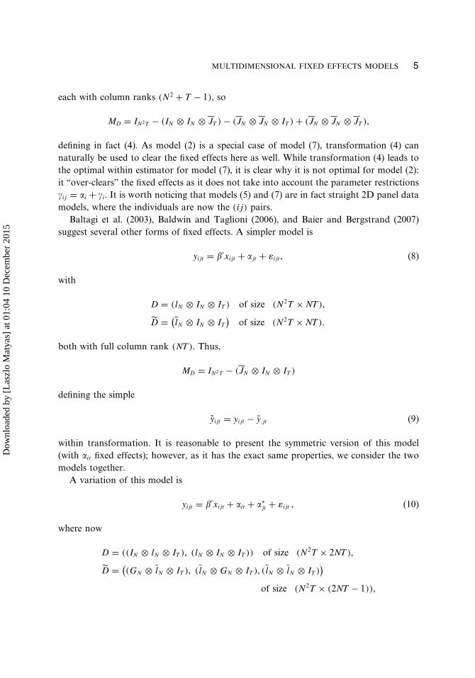
each with column ranks (N 2 + T − 1), so

MD = IN 2T − (IN ⊗ IN ⊗ �JT ) − (�JN ⊗ �JN ⊗ IT ) + (�JN ⊗ �JN ⊗ �JT ),

defining in fact (4). As model (2) is a special case of model (7), transformation (4) cannaturally be used to clear the fixed effects here as well. While transformation (4) leads tothe optimal within estimator for model (7), it is clear why it is not optimal for model (2):it “over-clears” the fixed effects as it does not take into account the parameter restrictions�ij = �i + �i. It is worth noticing that models (5) and (7) are in fact straight 2D panel datamodels, where the individuals are now the (ij) pairs.

Baltagi et al. (2003), Baldwin and Taglioni (2006), and Baier and Bergstrand (2007)suggest several other forms of fixed effects. A simpler model is

yijt = �′xijt + �jt + �ijt, (8)

with

D = (lN ⊗ IN ⊗ IT ) of size (N 2T × NT),

D = (lN ⊗ IN ⊗ IT

)of size (N 2T × NT)�

both with full column rank (NT). Thus,

MD = IN 2T − (�JN ⊗ IN ⊗ IT )

defining the simple

yijt = yijt − y�jt (9)

within transformation. It is reasonable to present the symmetric version of this model(with �it fixed effects); however, as it has the exact same properties, we consider the twomodels together.

A variation of this model is

yijt = �′xijt + �it + �∗jt + �ijt , (10)

where now

D = ((IN ⊗ lN ⊗ IT ), (lN ⊗ IN ⊗ IT )) of size (N 2T × 2NT),

D = ((GN ⊗ lN ⊗ IT ), (lN ⊗ GN ⊗ IT ), (lN ⊗ lN ⊗ IT )

)of size (N 2T × (2NT − 1)),

Dow

nloa

ded

by [

Las

zlo

Mat

yas]

at 0

1:04

10

Dec

embe

r 20

15

6 L. BALAZSI ET AL.

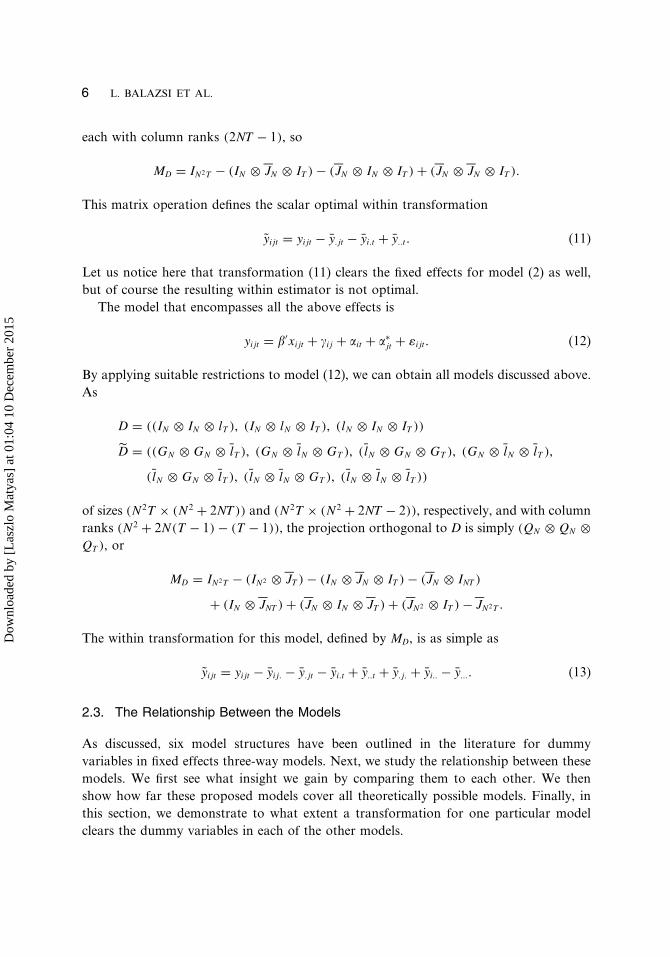
each with column ranks (2NT − 1), so

MD = IN 2T − (IN ⊗ �JN ⊗ IT ) − (�JN ⊗ IN ⊗ IT ) + (�JN ⊗ �JN ⊗ IT )�

This matrix operation defines the scalar optimal within transformation

yijt = yijt − y�jt − yi�t + y��t� (11)

Let us notice here that transformation (11) clears the fixed effects for model (2) as well,but of course the resulting within estimator is not optimal.

The model that encompasses all the above effects is

yijt = �′xijt + �ij + �it + �∗jt + �ijt� (12)

By applying suitable restrictions to model (12), we can obtain all models discussed above.As

D = ((IN ⊗ IN ⊗ lT ), (IN ⊗ lN ⊗ IT ), (lN ⊗ IN ⊗ IT ))

D = ((GN ⊗ GN ⊗ lT ), (GN ⊗ lN ⊗ GT ), (lN ⊗ GN ⊗ GT ), (GN ⊗ lN ⊗ lT ),

(lN ⊗ GN ⊗ lT ), (lN ⊗ lN ⊗ GT ), (lN ⊗ lN ⊗ lT ))

of sizes (N 2T × (N 2 + 2NT)) and (N 2T × (N 2 + 2NT − 2)), respectively, and with columnranks (N 2 + 2N (T − 1) − (T − 1)), the projection orthogonal to D is simply (QN ⊗ QN ⊗QT ), or

MD = IN 2T − (IN 2 ⊗ �JT ) − (IN ⊗ �JN ⊗ IT ) − (�JN ⊗ INT )

+ (IN ⊗ �JNT ) + (�JN ⊗ IN ⊗ �JT ) + (�JN 2 ⊗ IT ) −�JN 2T �

The within transformation for this model, defined by MD, is as simple as

yijt = yijt − yij� − y�jt − yi�t + y��t + y�j� + yi�� − y���� (13)

2.3. The Relationship Between the Models

As discussed, six model structures have been outlined in the literature for dummyvariables in fixed effects three-way models. Next, we study the relationship between thesemodels. We first see what insight we gain by comparing them to each other. We thenshow how far these proposed models cover all theoretically possible models. Finally, inthis section, we demonstrate to what extent a transformation for one particular modelclears the dummy variables in each of the other models.

Dow

nloa

ded

by [

Las

zlo

Mat

yas]

at 0

1:04

10

Dec

embe

r 20

15

MULTIDIMENSIONAL FIXED EFFECTS MODELS 7

To start with, let us make the structure of the models visible. A clear way to do thisis through the projection matrix DD′ = IN 2T − MD, which projects the data into the spacespanned by the dummy variables D. This matrix can be easily obtained, as D for eachmodel has already been written out explicitly. In elaborating DD′, we replace IN by QN +�JN and likewise for QT . Remember that �JN = lN l′N = lN l′N /N and QN = GN G′

N = IN −�JN .Results are presented in Table 1. Each column of the table corresponds to one particularmodel and a + sign indicates which building blocks have to be used to get the appropriateDD′.

We see that the first row of Table 1 is empty. Any model producing a DD′ with anonempty first row would indicate fixed effects with three indices, which evidently doesnot make sense for three-way data. The fact that the last row of the table does not haveempty cells means that all structures have effects that add up to one. The number ofmodels with an empty first row and a full last row is 26. As these models are nested intoat least one of the six models we cover, we take in fact care of all relevant cases.

Let us now address the question of the extent to which the transformation for onemodel clears the effects of another one. Model A does so for model B if, in obviousnotation, MADB = 0. In terms of Table 1, this is the case when the + signs of modelA cover those of model B. We see that the transformation of the “all-encompassing”model (12) covers all cases, while the transformations of model (10) covers only models(2) and (8), and so on. Another kind of insight from this exercise is into the possibleeffect of misspecification error(s). When, for example, the true model is (7) and we usethe transformation corresponding to model (10), the effects are not fully cleared, thusleading to a bias in the estimation of �. The argument can go the other way as well. If,for example, transformation (13) is used for model (5), we in effect “over-clear” the fixedeffects, thus leading to a loss of efficiency.

TABLE 1Building Blocks in Projection Matrices

(IN 2T −MD) = DD′

Model (2) (5) (7) (8) (10) (12)

QN ⊗ QN ⊗ QT

QN ⊗ QN ⊗ �JT + + +QN ⊗ �JN ⊗ QT + +�JN ⊗ QN ⊗ QT + + +QN ⊗ �JN ⊗ �JT + + + + +�JN ⊗ QN ⊗ �JT + + + + + +�JN ⊗ �JN ⊗ QT + + + + +�JN ⊗ �JN ⊗ �JT + + + + + +

Dow

nloa

ded

by [

Las

zlo

Mat

yas]

at 0

1:04

10

Dec

embe

r 20

15

8 L. BALAZSI ET AL.

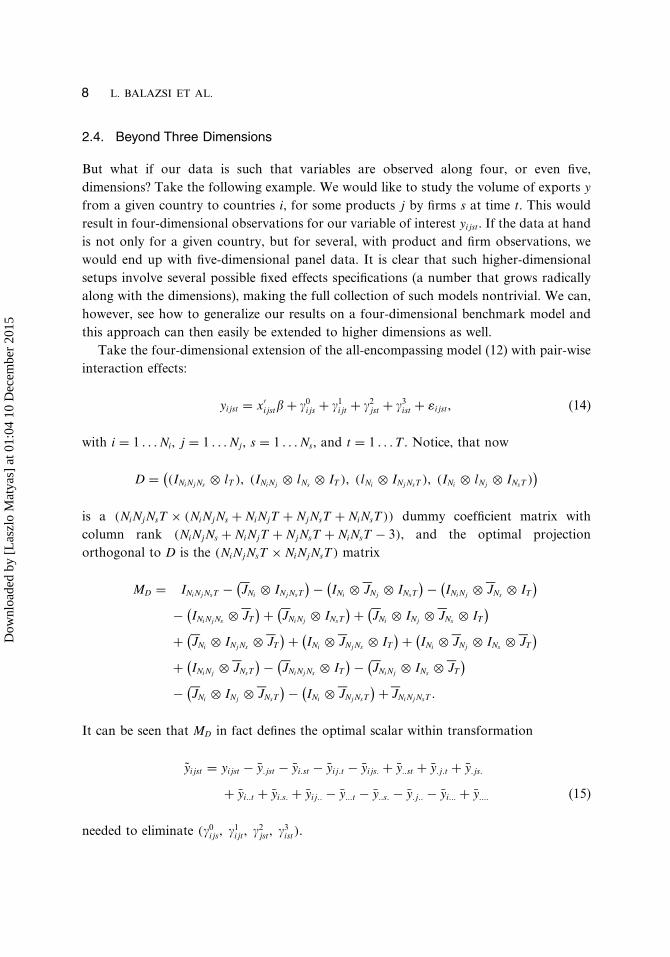
2.4. Beyond Three Dimensions

But what if our data is such that variables are observed along four, or even five,dimensions? Take the following example. We would like to study the volume of exports yfrom a given country to countries i, for some products j by firms s at time t. This wouldresult in four-dimensional observations for our variable of interest yijst. If the data at handis not only for a given country, but for several, with product and firm observations, wewould end up with five-dimensional panel data. It is clear that such higher-dimensionalsetups involve several possible fixed effects specifications (a number that grows radicallyalong with the dimensions), making the full collection of such models nontrivial. We can,however, see how to generalize our results on a four-dimensional benchmark model andthis approach can then easily be extended to higher dimensions as well.

Take the four-dimensional extension of the all-encompassing model (12) with pair-wiseinteraction effects:

yijst = x′ijst� + �0

ijs + �1ijt + �2

jst + �3ist + �ijst, (14)

with i = 1 � � � Ni, j = 1 � � � Nj , s = 1 � � � Ns, and t = 1 � � � T . Notice, that now

D = ((INiNj Ns ⊗ lT ), (INiNj ⊗ lNs ⊗ IT ), (lNi ⊗ INj NsT ), (INi ⊗ lNj ⊗ INsT )

)is a (NiNjNsT × (NiNjNs + NiNjT + NjNsT + NiNsT)) dummy coefficient matrix withcolumn rank (NiNjNs + NiNjT + NjNsT + NiNsT − 3), and the optimal projectionorthogonal to D is the (NiNjNsT × NiNjNsT) matrix

MD = INiNj NsT − (�JNi ⊗ INj NsT

) − (INi ⊗ �JNj ⊗ INsT

) − (INiNj ⊗ �JNs ⊗ IT

)− (

INiNj Ns ⊗ �JT

) + (�JNiNj ⊗ INsT

) + (�JNi ⊗ INj ⊗ �JNs ⊗ IT

)+ (�JNi ⊗ INj Ns ⊗ �JT

) + (INi ⊗ �JNj Ns ⊗ IT

) + (INi ⊗ �JNj ⊗ INs ⊗ �JT

)+ (

INiNj ⊗ �JNsT

) − (�JNiNj Ns ⊗ IT

) − (�JNiNj ⊗ INs ⊗ �JT

)− (�JNi ⊗ INj ⊗ �JNsT

) − (INi ⊗ �JNj NsT

) +�JNiNj NsT �

It can be seen that MD in fact defines the optimal scalar within transformation

yijst = yijst − y�jst − yi�st − yij�t − yijs� + y��st + y�j�t + y�js�

+ yi��t + yi�s� + yij�� − y���t − y��s� − y�j�� − yi��� + y���� (15)

needed to eliminate (�0ijs, �1

ijt, �2jst, �3

ist).

Dow

nloa

ded

by [

Las

zlo

Mat

yas]

at 0

1:04

10

Dec

embe

r 20

15

MULTIDIMENSIONAL FIXED EFFECTS MODELS 9

3. NO SELF-FLOW DATA

Often the models we study are used to deal with flow types of data like trade and capitalmovements (FDI) between countries. In such cases i and j index the same entities, Ni =Nj = N and there is, by definition, no self-flow. In terms of the models from Section 2, wehave a case of missing data and the transformations that we give can no longer be applied.Fortunately, the pattern of the missing observations is highly structured, allowing for thederivation of optimal transformations that are still quite simple. We start with presentingthe derivation of the optimal transformation for the T = 1 case in some detail as, to thebest of our knowledge, even this has not been studied in the literature. This leads us to theappropriate within transformation and also offers the main tools for deriving the optimaltransformation for all models from Section 2 with T > 1. The derivations are given in theonline supplement of this article.1

3.1. The Cross-Sectional Case

In the case when T = 1, there is only one relevant model. For i, j = 1, � � � , N ,

yij = �′xij + �i + �j + �ij , (16)

or in matrix form,

y = X� + (IN ⊗ lN )� + (lN ⊗ IN )� + �

≡ X� + D�� + D�� + �

≡ X� + D(�′, �′)′ + ��

As there are no data with i = j, we eliminate these from the model by using the selectionmatrix L of order N 2 × N (N − 1) to get

L′y = L′X� + L′D(�′, �′)′ + L′��

So the optimal effects-eliminating projection matrix is

ML′D = IN (N−1) − L′DW +D′L,

with W = D′LL′D and “+” denoting the Moore–Penrose generalized inverse. We want tohave a simple expression for the elements of ML′DL′y, indicated by a tilde. When in thedata i = j are observed, this expression is

yij = yij − yi� − y�j + y���

1See http://personal.ceu.edu/staff/matyas/BMW-Supplement.pdf

Dow

nloa

ded

by [

Las

zlo

Mat

yas]

at 0

1:04

10

Dec

embe

r 20

15

10 L. BALAZSI ET AL.

Now, the issue gets more complicated. For i �= j, (ei ⊗ ej)′D = (ei ⊗ ej)

′LL′D = (e′i, e′

j),so

yij = (ei ⊗ ej)′LML′DL′y

= yij − (e′i, e′

j)W +D′LL′y, (17)

with ei being the ith unit vector of size N . This causes us to further elaborate on W . Since

D′�LL′D� = D′

�LL′D� = (N − 1)IN and D′�LL′D� = JN − IN

and, as before, �JN = JN /N and QN = IN −�JN , we obtain

W =(

N − 1 −1−1 N − 1

)⊗ IN +

(0 11 0

)⊗ JN

=(

N − 1 −1−1 N − 1

)⊗ QN + (N − 1)

(1 11 1

)⊗ �JN �

Since QN and �JN are idempotent and mutually orthogonal, the Moore–Penrose inverseW + of W is

W + = 1N (N − 2)

(N − 1 1

1 N − 1

)⊗ QN + 1

4(N − 1)

(1 11 1

)⊗ �JN

= 1N (N − 2)

(N − 1 1

1 N − 1

)⊗ IN + 1

N

(p qq p

)⊗ JN ,

with

p = 14(N − 1)

− N − 1N (N − 2)

and q = 14(N − 1)

− 1N (N − 2)

�

Now, with this updated form of W ,

(e′i, e′

j)W + = 1N (N − 2)

((N − 1)e′

i + e′j , e′

i + (N − 1)e′j

) − 12(N − 1)(N − 2)

(l′N , l′N

)�

Moreover, with Y being the (N × N ) data matrix containing the yij observations, withzeros filling in the empty diagonal elements,

D′LL′y =(

Y ′lN

YlN

)�

Dow

nloa

ded

by [

Las

zlo

Mat

yas]

at 0

1:04

10

Dec

embe

r 20

15

MULTIDIMENSIONAL FIXED EFFECTS MODELS 11

So, after multiplying (e′i, e′

i)W + and D′LL′y, and as y++ = l′N YlN = l′N Y ′lN , we get

yij = yij − N − 1N (N − 2)

(yi+ + y+j

) − 1N (N − 2)

(y+i + yj+

)+ 1

(N − 1)(N − 2)y++� (18)

When N grows larger, the effects of the missing diagonal elements becomes smaller, whichis reflected in the above expression by the third term at the right-hand side of formula(18) being of lower order than N .

3.2. The Model with Three Effects

Let us turn our attention back to the three-dimensional models. To derive the optimalwithin transformation for model (2), we start from its matrix form

y = X� + (IN ⊗ lN ⊗ lT )� + (lN ⊗ IN ⊗ lT )� + (lN ⊗ lN ⊗ IT )� + �

= X� + D�∗� + D�∗� + D�� + ��

From this point, with D = (D�∗ , D�∗ , D�), the derivations are very similar to those usedfor pure cross-sections, only appearing slightly more complicated. The optimal withintransformation for model (2) in the no self-flow case is

yijt = yijt − N − 1N (N − 2)T

(yi++ + y+j+) − 1N (N − 2)T

(yj++ + y+i+)

− 1N (N − 1)

y++t + 2N (N − 2)T

y+++� (19)

3.3. Models with Composite Effects

Now, let us continue with the models with composite effects. In most cases, the optimalwithin transformation has to be adjusted only moderately, to reflect the missing diagonalelements. For model (5), this reads as

yijt = yijt − 1T

yij+; (20)

for model (7), it is

yijt = yijt − 1T

yij+ − 1N (N − 1)

y++t + 1TN (N − 1)

y+++; (21)

Dow

nloa

ded

by [

Las

zlo

Mat

yas]

at 0

1:04

10

Dec

embe

r 20

15

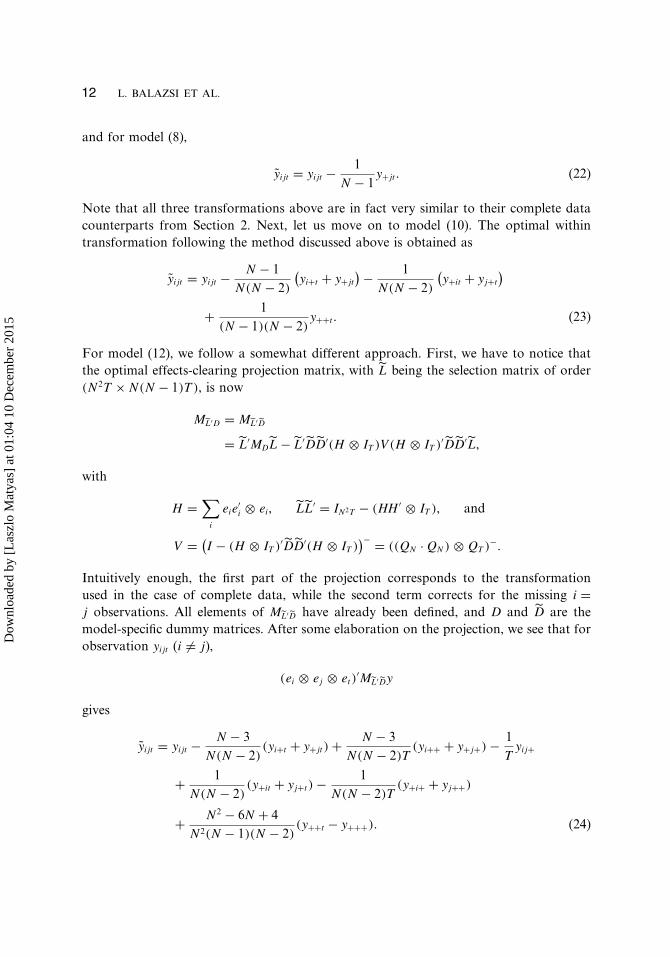
12 L. BALAZSI ET AL.

and for model (8),

yijt = yijt − 1N − 1

y+jt� (22)

Note that all three transformations above are in fact very similar to their complete datacounterparts from Section 2. Next, let us move on to model (10). The optimal withintransformation following the method discussed above is obtained as

yijt = yijt − N − 1N (N − 2)

(yi+t + y+jt

) − 1N (N − 2)

(y+it + yj+t

)+ 1

(N − 1)(N − 2)y++t� (23)

For model (12), we follow a somewhat different approach. First, we have to notice thatthe optimal effects-clearing projection matrix, with L being the selection matrix of order(N 2T × N (N − 1)T), is now

ML′D = ML′D

= L′MDL − L′DD′(H ⊗ IT )V (H ⊗ IT )′DD′L,

with

H =∑

i

eie′i ⊗ ei, LL′ = IN 2T − (HH ′ ⊗ IT ), and

V = (I − (H ⊗ IT )′DD′(H ⊗ IT )

)− = ((QN · QN ) ⊗ QT )−�

Intuitively enough, the first part of the projection corresponds to the transformationused in the case of complete data, while the second term corrects for the missing i =j observations. All elements of ML′D have already been defined, and D and D are themodel-specific dummy matrices. After some elaboration on the projection, we see that forobservation yijt (i �= j),

(ei ⊗ ej ⊗ et)′ML′Dy

gives

yijt = yijt − N − 3N (N − 2)

(yi+t + y+jt) + N − 3N (N − 2)T

(yi++ + y+j+) − 1T

yij+

+ 1N (N − 2)

(y+it + yj+t) − 1N (N − 2)T

(y+i+ + yj++)

+ N 2 − 6N + 4N 2(N − 1)(N − 2)

(y++t − y+++)� (24)

Dow

nloa

ded

by [

Las

zlo

Mat

yas]

at 0

1:04

10

Dec

embe

r 20

15

MULTIDIMENSIONAL FIXED EFFECTS MODELS 13

Note that this method is also flexibly applicable for all fixed effects model formulationsas one only has to substitute in the specific D and D dummy matrices corresponding tothe given model.

The listed no self-flow transformations can also be generalized to any higherdimensions. In the four-dimensional case, we get

yijst = yijst − 1N − 1

y+jst − 1N − 1

yi+st − 1Ns

yij+t − 1T

yijs+ + 1(N − 1)2

y++st

+ 1(N − 1)Ns

y+j+t + 1(N − 1)T

y+js+ + 1(N − 1)Ns

yi++t + 1(N − 1)T

yi+s+

+ 1NsT

yij++ − 1(N − 1)2Ns

y+++t − 1(N − 1)2T

y++s+ − 1(N − 1)NsT

y+j++

− 1(N − 1)NsT

yi+++ + 1(N − 1)2NsT

y++++ − 1(N − 1)NsT

yji++

+ 1(N − 1)T

yjis+ + 1(N − 1)Ns

yji+t − 1N − 1

yjist� (25)

So overall, the self-flow data problem can be overcome by using an appropriate withintransformation leading to an unbiased estimator.

Next, we go further along the above lines and see what is going to happen if theobservation sets i and j are different. If the two sets are completely disjoint, say forexample, if we are modeling export activity between the EU and APEC countries, for allthe models considered, the within estimators are unbiased, as the no self-flow problemdoes not arise. If the two sets are not completely disjoint, say for example in the caseof trade between the EU and OECD countries, when the no self-flow problem doesarise, we are faced with the same biases that are outlined above. Unfortunately, however,transformations (19), (23), and (24) do not work in this case, and there are no obvioustransformations that could be worked out for this scenario.

4. UNBALANCED DATA

As in the case of the usual 2D panel data sets (see Wansbeek and Kapteyn, 1989, orBaltagi, 2005, for example), just more frequently, one may be faced with a situation inwhich the data at hand is unbalanced. In our framework of analysis, this means that forall the previously studied models, in general t ∈ Tij , for all (ij) pairs, where Tij is a subsetof the index set t ∈ 1, � � � , T�, with T being chronologically the last time period in whichwe have any (i, j) observations. Note that two Tij and Ti′j′ sets are usually different, andalso let R = ∑

ij |Tij| denote the total number of observations, where |Tij| is the cardinalityof the set Tij (the number of observations in the given set).

For models (5) and (8), the unbalanced nature of the data does not cause any problem,the within transformations can be used, and they have exactly the same properties, as in

Dow

nloa

ded

by [

Las

zlo

Mat

yas]

at 0

1:04

10

Dec

embe

r 20

15

14 L. BALAZSI ET AL.

the balanced case. However, for models (2), (7), (10), and (12), we face some problems.As the within transformations fail to fully eliminate the fixed effects for these models(somewhat similarly to the no self-flow case), the resulting within estimators suffer from(potentially severe) biases. However, the Wansbeek and Kapteyn (1989) approach can beextended to these four cases.

Let us start with model (2). Dummy variable matrix D has to be modified to reflect theunbalanced nature of the data. Let the Ut and Vt (t = 1 � � � T ) be the sequence of (IN ⊗ lN )

and (lN ⊗ IN ) matrices, respectively, in which the following adjustments were made: foreach (ij) observation, we leave the row [representing (ij)] in those Ut and Vt matricesuntouched, are t ∈ Tij , but delete it from the remaining T − |Tij| matrices. In this way weend up with the following dummy variable setup:

Da1 = (

U ′1, U ′

2, � � � , U ′T

)′of size (R × N ),

Da2 = (

V ′1, V ′

2, � � � , V ′T

)′of size (R × N ), and

Da3 = diag V1 · lN , V2 · lN � � � , VT · lN � of size (R × T)�

So the complete dummy variable structure is now Da = (Da1 , Da

2 , Da3). In this case, let us

note here that, just as in Wansbeek and Kapteyn (1989), index t goes “slowly” and ijgoes “fast.” Now with this modified dummy variable structure, the optimal projectionremoving the fixed effects can be obtained in the following three steps:

M (1)Da

= IR − Da1(Da′

1 Da1)−1Da′

1 ,

M (2)Da

= M (1)Da

− M (1)Da

Da2(Da′

2 M (1)Da

Da2)−Da′

2 M (1)Da

,

and finally,

MDa = M (3)Da

= M (2)Da

− M (2)Da

Da3(Da′

3 M (2)Da

Da3)−Da′

3 M (2)Da

, (26)

where “−” stands for any generalized inverse. It is easy to see that in fact MDa Da =0 projects out all three dummy matrices. Note that in the balanced case (Da′

1 Da1)−1 =

IN /(NT), but now

(Da′1 Da

1)−1 = diag

{1∑

j |T1j| ,1∑

j |T2j| , � � � ,1∑

j |TNj|

}of size (N × N )�

With this in hand, we only have to calculate two inverses instead of three, (Da′2 M (1)

DaDa

2)−,and (Da′

3 M (2)Da

Da3)−, with respective sizes (N × N ) and (T × T ). This is feasible for

reasonable sample sizes.

Dow

nloa

ded

by [

Las

zlo

Mat

yas]

at 0

1:04

10

Dec

embe

r 20

15

MULTIDIMENSIONAL FIXED EFFECTS MODELS 15

For model (7), the job is essentially the same. Let the Wt (t = 1 � � � T ) be the sequenceof (IN ⊗ IN ) matrices, where again for each (ij), we remove the rows corresponding toobservation (ij) in those Wt, where t � Tij . In this way,

Db1 = (

W ′1, W ′

2, � � � , W ′T

)′of size (R × N 2),

Db2 = Da

3 of size (R × T)�

The first step in the projection is now

M (1)Db

= IR − Db1(Db′

1 Db1)

−1Db′1 ,

so the optimal projection orthogonal to Db = (Db1, Db

2) is simply

MDb = M (2)Db

= M (1)Db

− M (1)Db

Db2(Db′

2 M (1)Db

Db2)

−Db′2 M (1)

Db� (27)

Note that as

(Db′1 Db

1)−1 = diag

{1

|T11| ,1

|T12| , � � � ,1

|TNN |}

of size (N 2 × N 2),

we only have to calculate the inverse of a (T × T) matrix, Db′2 M (1)

DbDb

2, which is easilydoable. Further, as discussed above, given that model (2) is nested in (7), transformation(27) is in fact also valid for model (2).

Let us move on to model (10). Now, after the same adjustments as before,

Dc1 = diagU1, U2, � � � , UT � of size (R × NT) and

Dc2 = diagV1, V2, � � � , VT � of size (R × NT),

so the stepwise projection, removing Dc = (Dc1, Dc

2), is

M (1)Dc

= IR − Dc1(Dc′

1 Dc1)

−1Dc′1 ,

leading to

MDc = M (2)Dc

= M (1)Dc

− M (1)Dc

Dc2(Dc′

2 M (1)Dc

Dc2)

−Dc′2 M (1)

Dc� (28)

Note that for MDc , we have to invert (NT × NT) matrices, which can be computationallydifficult.

The last model to deal with is model (12). Let Dd = (Dd1 , Dd

2 , Dd3 ), where the adjusted

dummy matrices are all defined above:

Dd1 = Db

1 of size (R × N 2),

Dow

nloa

ded

by [

Las

zlo

Mat

yas]

at 0

1:04

10

Dec

embe

r 20

15

16 L. BALAZSI ET AL.

Dd2 = Dc

1 of size (R × NT),

Dd3 = Dc

2 of size (R × NT)�

Defining the partial projector matrices M (1)Dd

and M (2)Dd

as

M (1)Dd

= IR − Dd1 (Dd′

1 Dd1 )−1Dd′

1 and

M (2)Dd

= M (1)Dd

− M (1)Dd

Dd′2 (Dd′

2 M (1)Dd

Dd2 )−Dd′

2 M (1)Dd

,

the appropriate transformation for model (12) is now

MDd = M (3)Dd

= M (2)Dd

− M (2)Dd

Dd′3 (Dd′

3 M (2)Dd

Dd3 )−Dd′

3 M (2)Dd

� (29)

It can be easily verified that MDd is idempotent and MDd Dd = 0, so all the fixed effectsare indeed eliminated.2 As model (10) is covered by model (12), projection (29) eliminatesthe fixed effects from that model as well. Moreover, as suggested above, all three-wayfixed effects models are in fact nested into model (12). It is therefore intuitive thattransformation (29) clears the fixed effects in all model formulations. Using (29) is notalways advantageous, however, as the transformation involves the inversion of potentiallylarge matrices (of order NT ). In the case of most models studied, we can find suitableunbalanced transformations at the cost of only inverting (T × T) matrices; or in somecases, we can even derive scalar transformations. It is good to know, however, that there isa general projection that is universally applicable to all three-way models in the presenceof all kinds of data issues.

It is worth noting that transformations (26), (27), (28), and (29) are all dealing in anatural way with the no self-flow problem, as only the rows corresponding to the i = jobservations need to be deleted from the corresponding dummy variable matrices.

All transformations detailed above can also be rewritten in a semiscalar form. Let usshow here how this idea works on transformation (29), as all subsequent transformationscan be dealt with in the same way. Let

� = C−�D′y and = C−(M (2)Dd

Dd3 )′y � = C−�D′Dd

3 ,

where

C = (Dd

2

)′ �D, �D = (IR − Dd

1 (Dd′1 Dd

1 )−1Dd′1

)Dd

2 , and C = Dd′3 M (2)

DdDd

3 �

2A STATA program code for transformation (29) with a user-friendly detailed explanation is availableat www.personal.ceu.hu/staff/repec/pdf/stata-program_document-dofile.pdf. Estimation of model (12) is theneasily done for any kind of incompleteness.

Dow

nloa

ded

by [

Las

zlo

Mat

yas]

at 0

1:04

10

Dec

embe

r 20

15

MULTIDIMENSIONAL FIXED EFFECTS MODELS 17

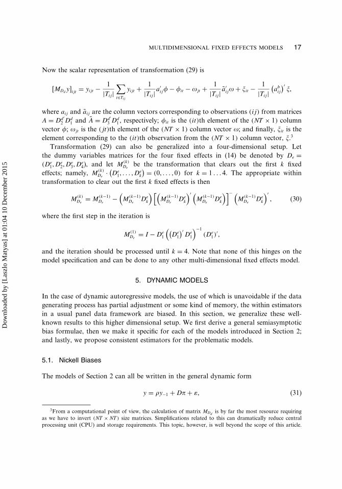
Now the scalar representation of transformation (29) is

�MDd y�ijt = yijt − 1|Tij|

∑t∈Tij

yijt + 1|Tij|a′

ij� − �it − jt + 1|Tij| a′

ij + �it − 1|Tij|

(ab

ij

)′�,

where aij and aij are the column vectors corresponding to observations (ij) from matricesA = Dd′

2 Dd1 and A = Dd′

3 Dd1 , respectively; �it is the (it)th element of the (NT × 1) column

vector �; jt is the (jt)th element of the (NT × 1) column vector ; and finally, �it is theelement corresponding to the (it)th observation from the (NT × 1) column vector, �.3

Transformation (29) can also be generalized into a four-dimensional setup. Letthe dummy variables matrices for the four fixed effects in (14) be denoted by De =(De

1, De2, De

3, De4), and let M (k)

Debe the transformation that clears out the first k fixed

effects; namely, M (k)De

· (De

1, � � � , Dek

) = (0, � � � , 0) for k = 1 � � � 4. The appropriate withintransformation to clear out the first k fixed effects is then

M (k)De

= M (k−1)De

−(

M (k−1)De

Dek

) [(M (k−1)

DeDe

k

)′ (M (k−1)

DeDe

k

)]− (M (k−1)

DeDe

k

)′, (30)

where the first step in the iteration is

M (1)De

= I − De1

((De

1

)′De

1

)−1(De

1)′,

and the iteration should be processed until k = 4. Note that none of this hinges on themodel specification and can be done to any other multi-dimensional fixed effects model.

5. DYNAMIC MODELS

In the case of dynamic autoregressive models, the use of which is unavoidable if the datagenerating process has partial adjustment or some kind of memory, the within estimatorsin a usual panel data framework are biased. In this section, we generalize these well-known results to this higher dimensional setup. We first derive a general semiasymptoticbias formulae, then we make it specific for each of the models introduced in Section 2;and lastly, we propose consistent estimators for the problematic models.

5.1. Nickell Biases

The models of Section 2 can all be written in the general dynamic form

y = �y−1 + D� + �, (31)

3From a computational point of view, the calculation of matrix MDd is by far the most resource requiringas we have to invert (NT × NT) size matrices. Simplifications related to this can dramatically reduce centralprocessing unit (CPU) and storage requirements. This topic, however, is well beyond the scope of this article.

Dow

nloa

ded

by [

Las

zlo

Mat

yas]

at 0

1:04

10

Dec

embe

r 20

15

18 L. BALAZSI ET AL.

where D and � correspond to any of the specific D and � discussed in Section 2. WithMD, the projection matrix orthogonal to D,

� = y′−1MDy

y′−1MDy−1

= � + tr(MD�y′−1)

tr(MDy−1y′−1)

, (32)

where y and y−1 are the column vectors of dependent and lagged dependent variables,respectively, of size N 2T . Let

B0 =(

0 0IT−1 0

)of size (T × T),

�0 ≡ (IT − �B0)−1 =

⎛⎜⎜⎜⎜⎝1 � � � � � � 0

�� � �

���� � �

� � ����

�T−1 � 1

⎞⎟⎟⎟⎟⎠ of size (T × T),

�0 =

⎛⎜⎜⎜⎜⎝1 � �T−1

�� � �

� � �

� � �� � � �

�T−1 � 1

⎞⎟⎟⎟⎟⎠ = IT + �(�0B0 + (�0B0)′) of size (T × T),

and let B = IN 2 ⊗ B0, � = IN 2 ⊗ �0, � = IN 2 ⊗ �0 define matrices necessary for the generalbias formulae. With e1, the first unit vector of size (T × 1), and y0 having N 2 elements[the initial values of the yijt for all (ij) pair],

By = y−1 − y0 ⊗ e1�

Therefore, model (31) can be rewritten as

y = �By + �y0 ⊗ e1 + D� + �, or (IN 2T − �B)y = �y0 ⊗ e1 + D� + �,

which ultimately leads to

y = ��(y0 ⊗ e1) + �D� + ���

Let �+ be � advanced by one time period. Then, under the stationarity of �ijt,

E(y−1�′) = E(y�′

+) = �E(��′+) = 2

��B�

So, for the expectation of the numerator in (32), we obtain

E(tr(MD�y′−1)) = 2

�tr(MD�B) = 2�

2�(tr(MD�) − tr(MD)),

Dow

nloa

ded

by [

Las

zlo

Mat

yas]

at 0

1:04

10

Dec

embe

r 20

15

MULTIDIMENSIONAL FIXED EFFECTS MODELS 19

with � = (IN 2T + �(�B + (�B)′)). For the denominator in (32),

E(tr(MDy−1y′−1)) = E(tr(MDyy′))

= �2E(tr(MDy−1y′−1)) + 2

�tr(MD) + 2E(tr(MD�y′−1)),

so, as E(tr(MD�y′−1)) = 2

�tr(MD�B),

E(tr(MDy−1y′−1)) = 2

�

1 − �2(tr(MD) + 2tr(MD�B)) = 2

�

1 − �2tr(MD�)�

Combining the expressions for the numerator and denominator, we get

plimN→∞

� = � + 1 − �2

2�

(1 − plim

N→∞tr(MD)

tr(MD�)

)� (33)

As for the specific models, given that tr(IT �0) = tr(IT ), the traces are summarized inTable 2.

� = tr(�JT �0) = 1 + 2�

1 − �

(1 − 1

T1 − �T

1 − �

)�

Therefore, following (33), the individual asymptotic biases are given in Table 3.

TABLE 2Traces for the Models Considered

Model tr(MD) tr(MD�)

(2) (N − 1)(NT + T − 2) (N − 1)(NT + T − 2�)

(5) N 2(T − 1) N 2(T − �)

(7) (N 2 − 1)(T − 1) (N 2 − 1)(T − �)

(8) NT(N − 1) NT(N − 1)

(10) (N − 1)2T (N − 1)2T(12) (N − 1)2(T − 1) (N − 1)2(T − �)

TABLE 3Asymptotic Biases for the Models Considered

ModelplimN→∞

� − �

(2)1 − �2

2�

(1 − plim

N→∞NT + T − 2

NT + T − 2�

)= 0

(5), (7), (12)1 − �2

2�

(1 − T − 1

T − �

)(8), (10) 0

Dow

nloa

ded

by [

Las

zlo

Mat

yas]

at 0

1:04

10

Dec

embe

r 20

15

20 L. BALAZSI ET AL.

5.2. Arellano–Bond Estimation

As seen above, we have problems with the N inconsistency of models (5), (7), and(12) in the dynamic case. Luckily, many of the well-known instrumental variables (IV)estimators developed to deal with dynamic panel data models can be generalized to thesehigher dimensions as well, as the number of available orthogonality conditions increasestogether with the dimensions. Let us take the example of one of the most frequently usedestimators: the Arellano and Bond IV estimator (see Arellano and Bond, 1991, and Harriset al., 2008, p. 260) for the estimation of model (5).

The model is written up in first differences, such as(yijt − yijt−1

) = �(yijt−1 − yijt−2

) + (�ijt − �ijt−1

), t = 3, � � � , T

or

�yijt = ��yijt−1 + ��ijt, t = 3, � � � , T �

The yijt−k, (k = 2, � � � , t − 1) are valid instruments for �yijt−1, as �yijt−1 is N asymptoticallycorrelated with yijt−k; however, yijt−k are not with ��ijt. As a result, the full instrument setfor a given cross-sectional pair, (ij) is

zij =

⎛⎜⎜⎜⎝yij1 0 · · · · · · 0 · · · 00 yij1 yij2 0 0 · · · 0��� · · · ���

��� · · · ���0 · · · 0 0 yij1 · · · yijT−2

⎞⎟⎟⎟⎠of size ((T − 2) × (T − 1)(T − 2)/2). The resulting IV estimator of � is

�AB =[�y′

−1ZAB

(Z′

AB�ZAB

)−1Z′

AB�y−1

]−1�y′

−1ZAB

(Z′

AB�ZAB

)−1Z′

AB�y,

where �y and �y−1 are the panel first differences, ZAB = (z′

11, z′12, � � � , z′

NN

)′, and � =

(IN 2 ⊗ �) is the covariance matrix, with known form

� =

⎛⎜⎜⎜⎜⎜⎝2 −1 0 · · · 0

−1 2 −1 · · · 0

0� � �

� � �� � � 0

0 · · · −1 2 −10 · · · 0 −1 2

⎞⎟⎟⎟⎟⎟⎠ of size ((T − 2) × (T − 2))�

The generalized Arellano–Bond estimator behaves in exactly the same way as the“original” two dimensional one, regardless of the dimensionality of the model.

In the case of models (7) and (12), to derive an Arellano–Bond–type estimator, weneed to insert one further step. After taking the first differences, we implement a simple

Dow

nloa

ded

by [

Las

zlo

Mat

yas]

at 0

1:04

10

Dec

embe

r 20

15

MULTIDIMENSIONAL FIXED EFFECTS MODELS 21

transformation in order to get to a model with only (ij) pairwise interaction effects,exactly as in model (5). We then proceed as above, as the ZAB instruments are valid forthese transformed models as well. Let us start with model (7) and take the first differencesto get

�yijt = ��yijt−1 + ��t + ��ijt�

Now, instead of estimating this equation directly with IV, we carry out the followingcross-sectional transformation:

�yijt =(

�yijt − 1N

N∑i=1

�yijt

),

or introduce the notation �y�jt = 1N

∑Ni=1 �yijt. We also notice that the �-s had been

eliminated from the model

(�yijt − �y�jt

) = �(�yijt−1 − �y�jt−1

) + (��ijt − ���jt

)�

We can see that the ZAB instruments proposed above are valid again for(�yijt−1 − �y�jt−1

),

as they are uncorrelated with(��ijt − ���jt

), but are correlated with the former. The IV

estimator of �, �AB has again the form

�AB = [�y′

−1ZAB(Z′AB�ZAB)−1Z′

AB�y−1

]−1�y′

−1ZAB(Z′AB�ZAB)−1Z′

AB�y,

with �y and �y−1 being the transformed panel first differences of the dependent variable.Continuing now with model (12), the transformation needed in this case is⎛⎝�yijt − 1

N

N∑i=1

�yijt − 1N

N∑j=1

�yijt + 1N 2

N∑i=1

N∑j=1

�yijt

⎞⎠ �

Picking up the previously introduced notation and using the fact that the fixed effects arecleared again, we get

(�yijt − �y�jt − �yi�t + �y��t)

= �(�yijt−1 − �y�jt−1 − �yi�t−1 + �y��t−1) + (��ijt − ���jt − ��i�t + ����t)�

The ZAB instruments can be used again on this transformed model to get a consistentestimator for �.

Dow

nloa

ded

by [

Las

zlo

Mat

yas]

at 0

1:04

10

Dec

embe

r 20

15

22 L. BALAZSI ET AL.

6. CONCLUSION

In the case of three and higher dimensional fixed effects panel data models, due tothe many interaction effects, the number of dummy variables in the models increasedramatically. As a consequence, even when the number of individuals and time periodsis not too large, the OLS estimator becomes, unfortunately, practically unfeasible. Theobvious answer to this challenge is to use appropriate within estimators, which do notrequire the explicit incorporation of the fixed effects into the model. Although thesewithin estimators are more complex than seen in the usual two dimensional panel datamodels, they are quite useful in these higher dimensional setups. However, unlike in twodimensions, they are biased in the case of some very relevant data problems, such asthe lack of self-flows or unbalanced observations. These properties must be taken intoaccount by all researchers relying on these methods. Also, in dynamic models, for some,but not all fixed effects formulations, the within estimators are biased and inconsistent.Therefore, appropriate estimation methods need to be derived to deal with these cases.

ACKNOWLEDGMENT

Last but not least, we would like to thank the editor and two anonymous reviewers fortheir very helpful comments that substantially improved the quality of the paper.

FUNDING

Support by the Australian Research Council grant DP110103824 is kindly acknowledged.Comments received from the participants of the 18th and 19th Panel Data Conferences,Paris 2012, and London 2013, respectively, are also much appreciated.

REFERENCES

Arellano, M., Bond, S. (1991). Some tests of specification for panel data: Monte-Carlo evidence and anapplication to employment equations. Review of Economic Studies 58:277–297.

Baier, S. L., Bergstrand, J. H. (2007). Do free trade agreements actually increase members international trade?Journal of International Economics 71:72–95.

Balestra, P., Krishnakumar, J. (2008). Fixed effects and fixed coefficients models. In: Matyas, L., Sevestre, P.,eds. The Econometrics of Panel Data. 3rd ed. Berlin, Heidelberg: Springer Verlag, pp. 23–48.

Baltagi, B. H., Egger, P., Pfaffermayr, M. (2003). A generalized design for Bilateral trade flow models.Economics Letters 80:391–397.

Baltagi, B. H. (2005). Econometric Analysis of Panel Data. 3rd ed. Chichester; Hoboken, NJ: John Wiley &Sons.

Baldwin, R., Taglioni, D. (2006). Gravity for dummies and dummies for the gravity equations. NBERWorking Paper 12516.

Cheng, I., Wall, H. J. (2005). Controlling for heterogeneity in gravity models of trade and integration. FederalReserve Bank of St. Louis Review 87(1):49–63.

Egger, P., Pfaffermayr, M. (2003). The proper econometric specification of the gravity equation: 3-Way modelwith bilateral interaction effects. Empirical Economics 28:571–580.

Dow

nloa

ded

by [

Las

zlo

Mat

yas]

at 0

1:04

10

Dec

embe

r 20

15

MULTIDIMENSIONAL FIXED EFFECTS MODELS 23

Gourieroux, C., Monfort, A. (1995). Statistics and Econometric Models. Cambridge: Cambridge UniversityPress.

Greene, W. H. (2012). Econometric Analysis. 7th ed. Prentice Hall, NJ: Pearson Education Ltd.Harris, M. N., Matyas, L., Sevestre, P. (2008). Dynamic models for short panels. In: Matyas, L., Sevestre,

eds. The Econometrics of Panel Data. 3rd ed. Berlin, Heidelberg: Springer Verlag.Matyas, L. (1997). Proper econometric specification of the gravity model. The World Economy 20:363–369.Nickell, S. (1981). Biases in dynamic models with fixed effects. Econometrica 49:1417–1426.Scheffé, H. (1959). The Analysis of Variance. New York: John Wiley & Sons.Wansbeek, T., Kapteyn, A. (1989). Estimation of error-components model with incomplete panels. Journal

of Econometrics 41:341–361.Wansbeek, T. (1991). Singular value decomposition of design matrices in balanced ANOVA models. Statistics

& Probability Letters 11:33–36.

Dow

nloa

ded

by [

Las

zlo

Mat

yas]

at 0

1:04

10

Dec

embe

r 20

15