University of PortlandPilot ScholarsEnvironmental Studies Faculty Publications andPresentations Environmental Studies

1-10-1990

Paleomagnetism of Middle Miocene VolcanicRocks in the Mojave-Sonora Desert Region ofWestern Arizona and Southeastern CaliforniaGary J. Calderone

Robert F. ButlerUniversity of Portland, butler@up.edu

Gary D. Acton

Follow this and additional works at: http://pilotscholars.up.edu/env_facpubs

Part of the Environmental Sciences Commons, Geology Commons, and the Geophysics andSeismology Commons

This Journal Article is brought to you for free and open access by the Environmental Studies at Pilot Scholars. It has been accepted for inclusion inEnvironmental Studies Faculty Publications and Presentations by an authorized administrator of Pilot Scholars. For more information, please contactlibrary@up.edu.

Citation: Pilot Scholars Version (Modified MLA Style)Calderone, Gary J.; Butler, Robert F.; and Acton, Gary D., "Paleomagnetism of Middle Miocene Volcanic Rocks in the Mojave-SonoraDesert Region of Western Arizona and Southeastern California" (1990). Environmental Studies Faculty Publications and Presentations.28.http://pilotscholars.up.edu/env_facpubs/28

JOURNAL OF GEOPHYSICAL RESEARCH, VOL. 95, NO. Bl, PAGES 625--647, JANUARY 10, 1990

Paleomagnetism of Middle Miocene Volcanic Rocks in the Mojave-Sonora Desert Region of Western Arizona and Southeastern California

GARY J. CALDERONE

U.S. Geological Survey, Flagstaff, Arizana

ROBERT F. BUTLER AND GARY D. ACTON 1

Department of Geosciences, University of Arizona, Tucson

Paleomagnetic directions have been obtained from 190 early to middle Miocene (12-20 Ma) mafic volcanic flows in 16 mountain ranges in the Mojave-Sonora desert region of western Arizona and southeastern California. These flows generally postdate early Miocene tectonic deformation accom­modated by low-angle normal faults but predate high-angle normal faulting in the region. After detailed demagnetization experiments, 179 flows yielded characteristic directions interpreted as original thermal remanent magnetizations (TRM). Because of the episodic nature of basaltic volcanism in this region, the 179 flows yielded only 65 time-distinct virtual geomagnetic poles (VGPs). The angular dispersion of the 65 VGPs is consistent with the angular dispersion expected for a data set that has adequately averaged geomagnetic secular variation. The paleomagnetic pole calculated from the 65 cooling unit VGPs is located at 85.5°N, 108.9°E within a 4.4° circle of 95% confidence. This pole is statistically indistinguishable (at 95% confidence) from reference poles calculated from rocks of similar age in stable North America and from a paleomagnetic pole calculated from rocks of similar age in Baja California. The coincidence of paleomagnetic poles from the Mojave-Sonora desert region with reference poles from the stable continental interior indicates that (I) significant vertical axis net tectonic rotations have not accompanied post-middle Miocene high-angle normal faulting in this region; (2) there has been no detectable post-middle Miocene latitudinal transport of the region; and (3) long-term nondipole components of the middle Miocene geomagnetic field probably were no larger than those of the recent (0--5 Ma) geomagnetic field. In contrast, paleomagnetic data indicate vertical axis rotations of similar age rocks in the Transverse Ranges, the Eastern Transverse Ranges, and the Mojave Block. We speculate that a major structural discontinuity in the vicinity of the southeastward projection of the Death Valley fault zone separates western areas affected by vertical axis rotations from eastern areas that have n_ot experienced such rotations.

INTRODUCTION

Beck [1976, 1980], Irving [1979], May et al. [1983], McWil/iams [1983], and Hillhouse and McWilliams [1987] have reviewed the extensive paleomagnetic evidence for clockwise rotations and northward translations of crustal fragments along the western margin of the North American Cordillera. The detection of large-scale latitudinal transla­tions [e.g., Hillhouse, 1977; Champion et al., 1984; Alvarez et al., 1980; Hillhouse and Gramme, 1984; Hag strum et al., 1985] has provided means by which to evaluate the paleo­geographies of tectonostratigraphic or suspect terranes [Co­ney et al., 1980]. The detection of vertical axis rotations largely unaccompanied by latitudinal translations (e.g., Or­egon-Washington Coast Range studies [Simpson and Cox, 1977; Magill and Cox, 1981; Magill et al., 1981; Gramme et al., 1986]) has provided means by which to evaluate the tectonic mechanisms and processes that might contribute to the geologic evolution of a region [Bates et al., 1981; Magill and Cox, 1981; Gromme et al., 1986; Wells and Heller. 1988].

Much attention has been given recently to the Miocene tectonic evolution of the southwestern United States [e.g.,

1Now at Department of Geological Sciences, Northwestern Uni­versity, Evanston, Illinois.

Copyright 1990 by the American Geophysical Union.

Paper number 89JB03216. 0148-0227 /90/89JB-03216$05. 00

625

Kamerling and Luyendyk, 1979, 1985; Luyendyk et al., 1985; Hagstrum et al., 1987b] (see Figure 1). Two features of the existing paleomagnetic data set for this region deserve special attention. The first is the geographic distribution and sense of discordant paleomagnetic declinations indicative of vertical axis tectonic rotation of crustal blocks. The second is the potential existence, geographic distribution, and mean­ing of discordant paleomagnetic inclinations.

Many workers [e.g., Luyendyk et al., 1985; Kamerling and Luyendyk, 1979, 1985; Hornafius et al. 1986] have presented data showing clockwise discordant paleomagnetic declina­tions from Miocene rocks west of the San Andreas fault in the Transverse Ranges of southern California. Carter et al. [1987] have shown evidence for clockwise discordant decli­nations in Miocene rocks of the Eastern Transverse Ranges east of the San Andreas fault. These clockwise discordant declinations have been interpreted to represent clockwise vertical axis tectonic rotation of crustal blocks bounded by northeast trending left-lateral strike-slip faults caught in the right-lateral shear between the Pacific and North American plates [Luyendyk et al., 1980, 1985].

Garfunkel [1974] predicted counterclockwise rotation of northwest trending faults in the Mojave Block (Figure I) on the basis of a kinematic analysis of the region. However, Luyendyk et al. [1980] predicted clockwise rotation of blocks bounded by east-west trending faults in this region. Coun­terclockwise discordant paleomagnetic declinations have been observed in the Mojave Block [Burke et al., 1982;

626 CALDERONE ET AL.: MOJAVE-SONORA DESERT PALEOMAGNETIC RESULTS

"~~'fo., \ i * :: ·. ~' \ i WH \. *Pl) * "-. * ~ CM_.:····· ...

COLORADO PLATEAU

CH I * ··· ..... * \ BM ······ CL ' ·· ..

' ·· ... ....

TRANSITK>N -.... * \ ·· .. · .. ···, I ZONE

T M ,... P A SONORA~············. Tr:= ) p L • SUBPROVINCE '··· ··•··

··. -134• ·········-···················i

· ..

', 1 , • K M J • Phoenla

.. , ~ /. ······················· ...

---,+,-;-~;!;;d.. c" 0 • G: A --- . . . 111• w

···,···. i 33•

Southern ·······' Basins and Ranges i

-....i, GR SM 114:--.......

• Tucaon • 0 I

100 MILES I

---1 -4~ 113~~~

~~o-......l 112;- .. .............._ _J

'-L----...l.----110• 1011• w

DB

111 •

Fig. I. Index map of the Mojave-Sonora desert region. Stars indicate ranges used in northern subregion. Circles are ranges used in southern subregion. See Table I for explanation of range symbols.

Acton, 1986] but may not have tectonic significance because of insufficient sampling of secular variation. In contrast, Golombek and Brown [1988], Ross et al. [1988, 1989], and MacFadden et al. [1990] observed clockwise discordant paleomagnetic declinations in Miocene rocks of this region. However, Hillhouse and Wells [1986] and Wells and Hill­house [1987, 1989] have found no regionally consistent pattern of tectonic rotation of the Peach Springs Tuff in a traverse from the Colorado Plateau to the vicinity of Bar­stow, California. In the Mojave Block, Wells and Hillhouse report small vertical axis rotations of both senses, appar­ently associated with strike-slip vaults in the region, as well as concordant directions. The combination of data sets has led Ross et al. [1989] and MacFadden et al. [1990] to propose a model suggesting that the Mojave Block has experienced two rotational episodes. The first episode oc­curred prior to the emplacement of the Peach Springs Tuff and produced clockwise vertical axis rotations. The second episode occurred after emplacement of the Peach Springs Tuff and produced rotations in both senses [Ross et al., 1989; MacFadden et al., [1990].

Further to the east, Wells and Hillhouse [1989] report significant vertical axis rotation of the Peach Springs Tuff associated with detachment terranes in the Colorado River trough. Both clockwise and counterclockwise rotations are observed and have been interpreted to be local rotation in the upper plates of the detachment faults. Costello [1985] reports a small clockwise rotation of Oligocene to early Miocene volcanic rocks in the Chocolate Mountains area of southeastern California. Calderone and Butler [1984] ob­served -a counterclockwise declination discordance, barely significant at the 95% confidence level, in Miocene rocks of southwestern Arizona and speculated that this discordance could be interpreted as tectonic rotation. However, Veseth et al. [1982] and Hagstrum et al. [1987a) observed no

significant declination discordance for the same area [see also Butterworth 1984; Callian, 1984; Costello, 1985; Veseth, 1985]. Geissman [1986] observed significant counterclock­wise discordant declinations in Miocene rocks of the Lake Mead region of northwest Arizona and southern Nevada, interpreting this deflection as local tectonic rotations along large shear zones.

The Colorado Plateau is considered to be part of the stable North American craton during Miocene time, although Bryan and Gordon [1986] have shown evidence for a small (3°-5°), post-middle Cretaceous clockwise rotation of this region consistent with the proposal of Hamilton [1981]. Kluth et al. [1982] and May et al. [1986] present evidence for little to no post-Middle Jurassic rotation of southeastern Arizona, and Vugteveen et al. [1981] and Barnes and Butler [1980] present paleomagnetic evidence from Late Creta­ceous and Paleocene rocks in southeastern Arizona implying no post-Paleocene rotation relative to cratonic North Amer­ica. Thus the general pattern that emerges is one of no discordant declinations in Miocene rocks of the eastern part of the southwestern United States, generally clockwise discordant declinations in the Eastern Transverse Ranges and west of the San Andreas fault, and discordances in both rotational senses from domains in the intervening southern Basin and Range.

Luyendyk et al. [ l 985 J examined the paleomagnetic incli­nation data from Miocene rocks in southern California and southwestern Arizona and concluded that inclinations are shallower than expected for an axial geocentric dipole model for the Miocene geomagnetic field. Morris et al. [1986] concluded that shallow inclinations west of the San Andreas fault could be interpreted as actual post-Miocene latitudinal translation of the Baja Borderland terrane greater than that which is attributable to the San Andreas transform. How­ever, this interpretation has been challenged by Hagstrum et

C'AI OERONE ET AL.: MOJAVE-SONORA DESERT PALEOMAGNETIC RESULTS 627

TABLE I. General Section Information

Latitude, Longitude, N/ Age,b Section ON OE Na Ma Lithology Symbol References d s

Black Mtns. 34.93 245.77 11/88 <18.3 basalte BM c Cerbat Mtns. 35.21 245.87 21/168 >18.3 basalte CM c Clipper Mtns. 34.75 244.57 9173 -17.0 basalt CL c Colton Hills 34.98 244.57 1113 15.5 tu ff CH D Piute Range 35.22 244.97 12173 14.2 andesite PI G Turtle Mtns. 34.30 245.23 10/61 15.9 basalt TM H White Hills 35.70 245.80 13/104 8.5 basalt WH I Castle Dome 33.00 246.02 21/159 -18.0 basalt CD B Del Bae Hills 32.30 249.00 6/49 23.5 basalt DB E Gila Bend 33.05 246.87 8/64 -18.0 basalt GB F&I Kofa Mtns. 32.38 246.10 7/51 18.3 basalt KM B Growler Mtns. 32.25 247.00 22/172 14.4 basalt GR A Little Ajo Mtns. 32.30 247.25 20/161 15.4 basalt LA A Sauceda Mtns. 32.50 247.50 12/96 20.I basalt SM A Plomosa Mtns. 33.50 246.00 9172 17.2 basalt PL B Parker Area 34.16 246.00 8/63 16.1 basalt PA B

For more detailed information regarding location, age and lithology, see Acton (1986] and Appendix I of Calderone (1988]. Total of 1467 samples from 190 sites in 16 ranges.

a Nf is the number of distinct flows sampled. Ns is the number of individually oriented samples taken in that section. b Age Ma is abbreviation for millions of years before present. csymbol is the designator used in subsequent tables and Figure I to identify samples and sites belonging to a particular section. dReference for age: A, Gray and Miller [1984]; B, Shafiqul/ah et al. (1980]; C, Glazner et al. (1986]; D, McCurry (1986]; E, Percious

(1968]; F, Eberly and Stanley (1978]; G, Spencer [1985]; H, Davis et al. (1982]; I, R. J. Miller (personal communication, 1988). eThe lowest sampled flow in the Black Mountains section and the highest sampled flow in the Cerbat Mountains are the Peach Springs

Tuff (J. Neilson, personal communication, 1988).

al. [1987b), who, using a larger data set, concluded that there is no evidence for such latitudinal motion of the Baja Borderland. Paleomagnetic inclinations from Miocene rocks of the Mojave Block [Golombek and Brown, 1988] are generally not discordant.

Two major questions about the existing paleomagnetic data set from Miocene rocks of the southwestern United States must be answered before a satisfactory model for the tectonic evolution and paleogeographic reconstruction can be formed: (1) What is the geographic distribution of discor­dant paleomagnetic declinations in the southwestern United States? (2) Do discordant paleomagnetic inclinations exist in the southwest United States, and if so, what is their geo­graphic distribution and what do they mean? Both questions require additional paleomagnetic data from the Mojave­Sonora desert region of the southern Basin and Range. This paper presents the results of a project undertaken to obtain paleomagnetic data from middle Miocene basalts in the southern Basin and Range and attempts to answer these questions.

GENERAL GEOLOGY

The southwestern United States part of the North Amer­ican Cordillera comprises four physiographic provinces [Stewart, 1978): (I) the Colorado Plateau; (2) the southern Basin and Range; (3) the Transverse Ranges; and (4) the Peninsular Ranges (Figure 1). The southern Basin and Range can be further subdivided into three subprovinces on the basis of similar present-day geologic features: the Mojave Block; the southern Basin and Range; and the Sonoran subprovince [Aldridge and Laughlin, 1983) of the Basin and Range from which our collections were made (Figure 1). Several syntheses cover the regional tectonics of this region [e.g., Atwater, 1970;

Stewart, 1978; Thompson and Burke, 1973; Coney, 1978; Burchfiel and Davis, 1981; Dickinson, 1981).

Pre-Quaternary rocks in the Mojave-Sonora desert are exposed almost exclusively in the mountain ranges. The youngest of the pre-Quaternary are typically middle Mi­ocene volcanic and volcaniclastic rocks. The volcanic rocks are typically basaltic in composition with subordinate andes­ites, dacites and tuffs [e.g., Luedke and Smith, 1978; Chris­tiansen and Lipman, 1977; Best et al., 1980). These rocks range in age from about 20 to 10 Ma (Table 1). They are typically flat-lying (less than 7° dip) and are usually deformed only by apparently high-angle, normal separation faults. These faults commonly trend northwest parallel to the mountain ranges [Spencer and Reynolds, 1986; Stewart 1978). Alteration is generally minimal. The basalts that we have sampled for this study usually occur as multiple flows in stratigraphic succession separated by volcanic breccia and scoria zones. These basaltic sequences unconformably over­lie older silicic and basaltic volcanic rocks and/or much older (pre-Oligocene) sedimentary and metamorphic rocks.

The older silicic and basaltic volcanic rocks in most places occur in tilt blocks associated with early to middle Miocene detachment faults. However, the space-time relationships between the older detachment faulting and the younger high-angle faulting are complex. In the Colorado River area, for example, the Peach Springs Tuff is tilted by detachment faulting, whereas in the nearby Cerbat Mountains, the Peach Springs Tuff and the underlying basalts are cut only by high-angle faults. Throughout the sample region, we have exclusively sampled sequences that were unaffected by or postdate the detachment faulting event.

Post-middle Miocene strike-slip faults are known in both the Mojave Block and the Lake Mead region. The strike-slip

628 CALDERONE ET AL.: MOJAVE-SONORA DESERT PALEOMAGNETIC RESULTS

components (if any) of high-angle faults in the southern Basin and Range are largely unknown.

FIELD AND LABORATORY METHODS

We have collected oriented samples from stratified se­quences of Miocene volcanic rocks in each of 16 mountain ranges in the southern Basin and Range. Range locations are shown on Figure 1 and are given in detail by Acton [1986] and in Appendix 1 of Calderone [1988]. Table 1 briefly summarizes the pertinent information.

We have sampled only volcanic rocks, as they are typi­cally the most accurate recorders of ancient magnetic fields and are both common and well exposed in the southern Basin and Range. We chose sequences that met the follow­ing criteria:

Structural simplicity. We would like to know that a paleomagnetic direction obtained from a particular mountain range is applicable to a structural domain of at least the size of that range. For this reason we have sampled essentially flat-lying (dipping less than 7°, with the exception of the Castle Dome Mountains section, which dips 10°) volcanic sequences that are internally unfaulted. Many of the ranges are probably bounded by faults that cut the volcanic se­quences.

Numerous flows in stratigraphic succession. It is critical to evaluate whether or not a particular set of volcanic flows has been extruded over a time sufficient to average geomag­netic secular variation; that is, the data should fully repre­sent a period of at least 10,000 years. Flows in stratigraphic succession allow us to evaluate the directional independence of adjacent flows.

Age control from isotopic dating. We have chosen to restrict our investigation to middle Miocene rocks and to only volcanic sequences with some isotopic dating available. In addition, age control aids comparisons between ranges and allows possible time variations in paleomagnetic direc­tional discordances to be investigated.

Our sampling scheme was designed to provide a continu­ous set of data covering the area from the Colorado Plateau/ southeastern Arizona to the areas previously or concurrently covered by Luyendyk et al. [1985], Hagstrum et al. [1987b], and Golombek and Brown [1988]. We collected sites from a transect that extends essentially from Kingman, Arizona, to the Clipper Mountains, 80 miles east of Barstow, California. In addition, we collected additional sites from the area previously sampled by Calderone and Butler [1984], a transect from Tucson, Arizona, to the Yuma, Arizona, region.

Six to thirteen individually oriented samples from each of 190 distinct flows in the sixteen ranges were collected using standard paleomagnetic coring techniques. Prior to drilling, outcrops were surveyed with a magnetic compass to detect areas of anomalously high magnetic intensity imparted by local lightning strikes. Areas where compass deflections were noted were avoided in sample collection. Azimuthal orientation for most samples (90%) was determined using both Sun and magnetic compasses. For those samples where solar orientations were not available, the magnetic azimuth was checked using the back azimuth technique.

In the Cerbat Mountains, a fine-grained volcaniclastic sedimentary unit is sandwiched between flows CMO 17 and CM018. The attitude of this bed (strike = 100°, dip = 7°S) is

used as the tectonic correction for flows CM001-CM017. There is no evidence to indicate that flows 18-21 have been similarly tilted, so flows CM018-CM021 have no tectonic correction. A similar situation exists in the Black Mountains, where a thin, fine-grained volcaniclastic unit is sandwiched between flows BM007 and BM008. The attitude of this unit (strike = 320°, dip = 7°S) is used as a tectonic correction for flows BM001-BM007, while flows BM008-BM011 are essen­tially flat-lying.

In the Castle Dome Mountains, tectonic corrections were made using the 10° eastward tilt (305° strike) of the bedding planes between flows because geologic field observations of uniform flow thicknesses and nonhorizontal vesicle flat­tening render this amount of tilt unlikely to be primary. Because the tilt is small, however, the choice of whether or not to correct the Castle Dome directions makes essentially no difference in the final analysis. No tectonic correction is used for the remaining 13 sections, as no sedimentary beds could be found and the sections are flat-lying.

In the laboratory, one to five specimens of 2.4-cm length were cut from each of the 2.5-cm-diameter core samples. Measurement of the initial natural remanent magnetization (NRM) of each specimen was made using a Schonstedt SSM-lA spinner magnetometer. In an effort to identify and segregate components of NRM, two or three specimens from each site (flow) were subjected to stepwise progressive alternating field (AF) demagnetization treatment using a Schonstedt GSD-5 tumbling specimen AF demagnetizer. Peak fields ranged from 1.2 millitesla (mT) to 100 mT. In addition, one specimen each from selected sites was sub­jected to stepwise progressive thermal demagnetization treatment in a mu-metal shielded furnace with a field of <10 nanotesla (nT). Peak furnace temperatures ranged from 200°C to 600°C. Based on these results, the remaining specimens were progressively demagnetized at two or more steps.

ROCK MAGNETIC ANALYSIS

Observations of initial NRM directions and behavior dur­ing both partial AF demagnetization and thermal demagne­tization treatments allow classification of remanence into three major groups. These groups are here designated types A, B, and C. Type A remanence is interpreted as an uncomplicated, original thermal remanent magnetization (TRM). Type B remanence is a TRM overprinted by a weak to moderate lightning-induced isothermal remanent magne­tization (IRM). Type C remanence is a TRM overprinted by a strong, lightning-induced IRM.

Typical type A specimen directions show very little dis­persion, and progressive AF demagnetization treatment of type A specimens shows mostly the decay of only a single component of magnetization. Thermal demagnetization be­havior is similar to that of AF demagnetization. We interpret the characteristic remanence (ChRM) of type A specimens to be a TRM imparted to the specimens at the time of their initial cooling. Little or no secondary component of magne­tization is present.

Initial NRM directions of type B specimens show moder­ate to high intrasite dispersion (Figure 2a). Initi~l NRM intensities are typically 5-10 times higher than those of type A sites. Progressive AF demagnetization (Figure 2b) reveals a low to moderate coercivity component (removed using

CALDERONE ET AL.: MOJAVE-SONORA DESERT PALEOMAGNETIC RESULTS 629

0 .• A

•

• 270 >--1--+-+--+--+---+--+--+---<>--.__+--+--+--+--+-+->--1 90

• Lower he1isphere

TM003

before

de mag n e tlz at lo n

150

180

A Upper he1isphere

180

TM003

a ft er

demagnetization

• Lower hnisphere A Upper hnisphere

120

B TM003E (H)

UP, N

HORIZ.. E

DOWN, S

10 Alm

a INCLINATION A DECLINATION

TM003E IHI

UP, N c

HORIZ., E

~-------< • 2.5 Alm

a INCLINATION A DECLINATION

Fig. 2. Magnetic behavior of Type B specimens. (a) Equal-area projection of individual specimen NRM directions from a single flow in the Turtle Mountains prior to magnetic cleaning experiments. (b) Vector plot of NRM directions for a single specimen from that flow during progressive AF demagnetization. (c) Expanded view of the central portion of Figure 2b. (d) Equal-area projection of individual ChRM directions from the same flow after partial AF demagnetization. Note that a secondary component of erratic direction and high initial intensity is removed, isolating the characteristic NRM direction. The secondary component is most likely a lightning-induced IRM.

peak fields to 5 mT) and a high coerc1V1ty (> 10 mT) characteristic component. The low-coercivity component is of high intensity and typically has no coherent intrasite direction. This component is most likely an IRM imparted by nearby lightning strikes. The intrasite dispersion of the high coercivity component is quite low (Figure 2d). Conse­quently, the high coercivity ChRM is most likely a TRM imparted to the rock at the time of extrusion and cooling.

Initial NRM directions of type C specimens show wide intrasite scatter. Initial intensities are also 5-10 times higher than those of type A (in some cases even higher). Partial AF demagnetization of such specimens shows evidence for two or more components of magnetization of similar coercivity spectra. Consequently, intrasite dispersion of NRM direc­tions did not decrease significantly during the AF treat­ments. Thermal demagnetization was not attempted on such

630 CALDERONE ET AL.: MOJAVE-SONORA DESERT PALEOMAGNETJC RESULTS

specimens but would not likely produce superior results. Sites in the Del Bae Hills and Gila Bend area contained only type C specimens. Additionally, several sites in the remain­ing ranges contained only such specimens.

We believe that type C remanence is composed of one or more IRMs imparted by very near, direct, or multiple lightning strikes. Most of these sites are atop high ridges likely to be exposed to lightning. Although an original TRM probably exists, it is not easily isolated. Although principal component analytical techniques described by Kirschvink [1980], Halls [1976], and Hoffman and Day [1978] might be used to extract the original TRM directions, their small number relative to the size of the rest of the sample collec­tion seemed to render such methods inexpedient except in the Del Bae Hills, the Gila Bend area, and the Kofa Mountains. In the former cases, we have simply eliminated these specimens from further consideration. In the latter three ranges we have applied principal component analysis [Kirschvink, 1980] in an attempt to obtain at least some paleomagnetic directional information.

The ChRM components of types A and B remanences usually have blocking temperatures which do not exceed 600°C. This observation, combined with the behavior during AF demagnetization, indicates that magnetite is the principal carrier of the remanence in these rocks.

In summary, out of 1806 specimens from 1467 samples taken from 190 sites, specimens from 1243 samples from 179 sites contain a ChRM direction that estimates the direction of the geomagnetic field at the time of original cooling of the flows.

PALEOMAGNETIC ANALYSIS

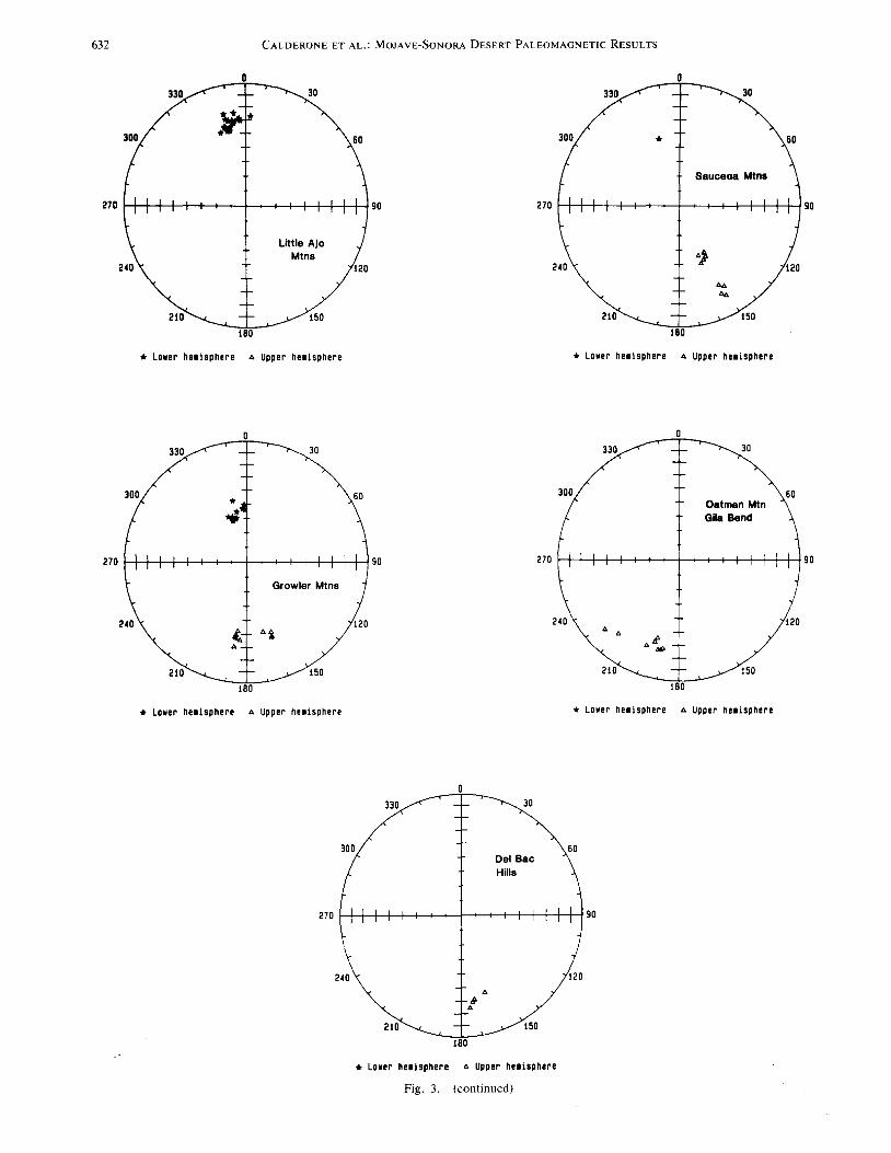
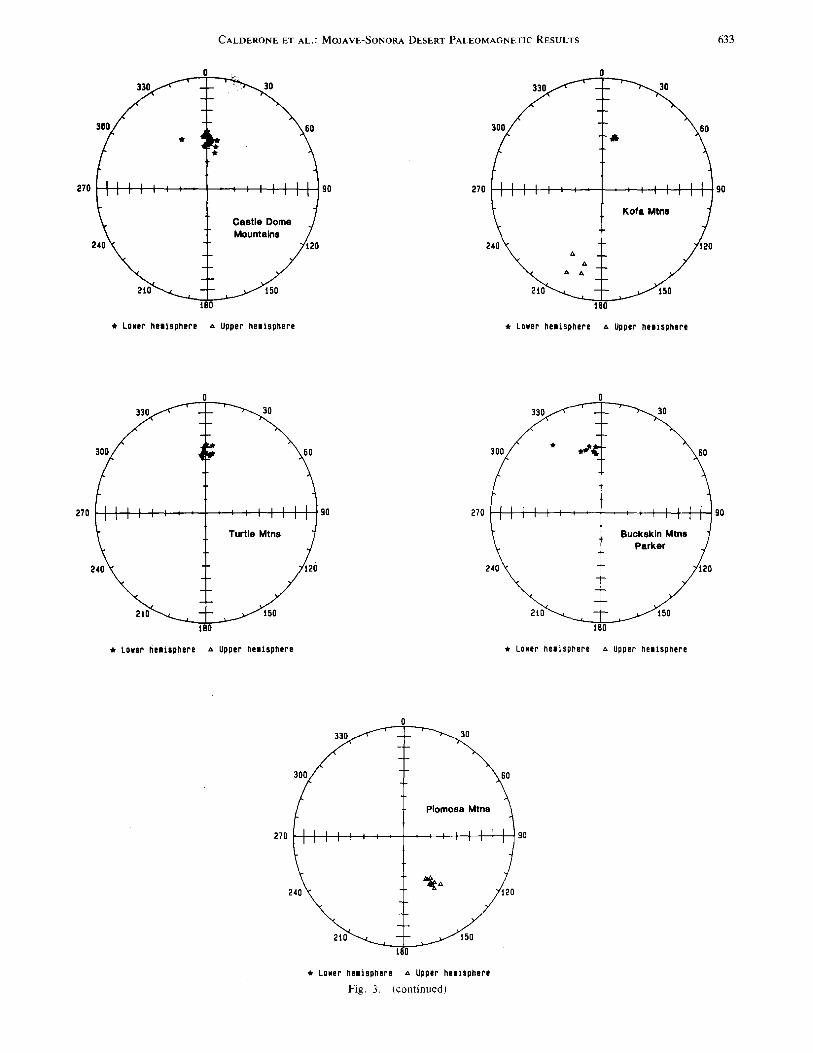
The appendix contains a detailed description of the meth­ods we have used to determine (I) the best estimate of ChRM direction within a single sample, (2) site mean ChRM directions and virtual geomagnetic poles (VGPs), (3) direc­tional independence of directions/VGPs from adjacent flows, and (4) whether or not a particular set of data fits the Fisher [1953] distribution and adequately samples geomagnetic sec­ular variation. Site mean directions (Figure 3) and VGPs are given in Table 2. The 179 mean flow directions yield only 65 independent measurements of the Miocene geomagnetic field (Table 3 and Figure 4).

Given the stringent criteria that we have adopted for tests of secular variation averaging, none of the individual ranges are particularly suited for testing because the number of individual cooling units is usually less than 10 and often less than five. This fact, in itself, suggests that volcanic extrusion in any given range is generally too episodic to afford an adequate temporal averaging of the geomagnetic field. More­over, as discussed by Calderone [1988], within each range either or both the dispersion or the distribution of directions/ VGPs are insufficient to ensure that geomagnetic secular variation will be adequately averaged out in the process of calculating a mean direction/pole. Therefore we cannot use our results from any individual range to measure rotations relative to the craton or to compare rotations between ranges .. Consequently, we have merged the direction/VGP data into ·a single set and analyzed the region as a tectonic domain.

The merged set of cooling unit mean directions/VGPs is plotted in Figure 4. We have reapplied secular variation

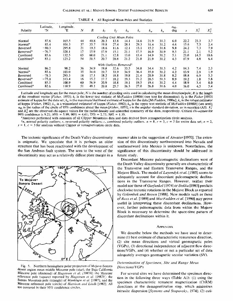
averaging tests to this new data set in pole space. Statistics for these latter tests are listed in Table 4. As shown in the appendix, this merged set of cooling unit VGPs adequately averages the Miocene paleosecular variation. Consequently, we have no reason to reject the idea that the mean pole from the combined polarity data is a paleomagnetic pole repre­sentative of the position of the Earth's rotation axis with respect to the Mojave-Sonora desert region during the Mi­ocene (about 12-20 Ma). The position of this pole is 85.5°N, 108.9°E and has a 95% confidence cone of 4.4° radius (see Figure 5).

It is possible that by analyzing the paleomagnetic data for the Mojave-Sonora desert region, we have averaged out important distinctions in directions that may be associated with subregions. Indeed, initial collection was guided by the idea that there may be a distinct discordance from the region originally collected by Calderone and Butler [1984]. To test for such potential internal differences in paleomagnetic di­rections/VGPs, we have divided the region into two subre­gions: (I) the southern subregion of southwestern Arizona and (2) the northern subregion of northwestern Arizona and southeastern California. The two subregions overlap in the area of the Turtle and Buckskin mountains (Parker area). It should be noted that the results of this comparison are essentially the same whether the Turtle and Buckskin moun­tains are grouped together in either the north or south subregion or are split into different subregions.

The results of this comparison are given in detail by Calderone [1988]. Although there is a slight discordance (mostly in declination) between the mean pole from the southern subregion and that of the northern subregion, this discordance is most likely due to the inability of cooling units in either subregion to actually average paleosecular varia­tion. The lack of secular variation averaging in the subre­gions attests to the episodic nature of the extrusion of basaltic flows in the latest phase of volcanism in the Mojave­Sonora desert. Because of this rapid extrusion, conclusions regarding the tectonic or paleomagnetic significance of re­sults from any part of the region must be based on a very large number of cooling units in a significant number of individual ranges.

CONCLUSIONS AND TECTONIC IMPLICATIONS

Virtual geomagnetic poles from Miocene cooling units in 16 mountain ranges in the Mojave-Sonora desert region yield a paleomagnetic pole at 85.5°N, 108.9°E within a 4.4° circle of 95% confidence. The VGPs appear to average out the secular variation of the Miocene geomagnetic field using the 0--5 Ma geomagnetic field as a model. We see no reason to reject the idea that the angular dispersion of the Miocene geomagnetic field is similar to that of the Pliocene to Ho­locene geomagnetic field (see the appendix).

The paleomagnetic pole from the Mojave-Sonora desert is not statistically different from the pole determined by Hag­strum et al. [1987b] from rocks of similar age in the Baja California region (Figure 5). Furthermore, the new pole is statistically indistinguishable at 95% confidence from the North American Miocene reference poles of Irving [1979], Irving and Irving [1982], and Harrison and Lindh [1983]. and a reference pole calculated by Hagstrum et al. [1987b]. Our pole is also statistically indistinguishable from the pole from . the High Lava Plains of Oregon as reported by Mankinen et

CALDERONE ET AL.: MOJAVE-SONORA DESERT PALEOMAGNETIC RESULTS 631

• •

270 l--l-+-+--+-+-+-+--t--1--1--11--1-+-+-+-i 90

Black Mtns Cerbat Mtna

• Lower hHlsphere "" Upper hemisphere • Lower hemisphere "" Upper h11lsphere

0

300 60

Piute Range

270 t-i-+-+-t--t--t--t---t---+-+-+-t--t--t-1-1 90 270 l--l-+--+-+--+--+--+---+---t--t--+--+-+-+-+-190

White Hilla Colton Hiia'-. ... ,. .........

150 210

180 180

• Lower heailphere "" Upper h11lsphere • Lower hemisphere "" Upper hemisphere

0

• • • 270 .. 90

Clipper Mtna

240 120

150

180

• Lower h11isphere "" Upper hHisphere

Fig. 3. Equal-area projections of cleaned site mean directions for each mountain range. Note clusters of flow directions in ranges such as the Black or Sauceda Mountains. These clusters correspond to flows that were probably extruded rapidly with respect to the secular variation of the geomagnetic field.

632

270

300

270

240

CALDERONE ET AL.: MOJAVE-SONORA DESERT PALEOMAGNETIC RESULTS

0

30

*

90 270

Little Ajo Mtns

!20 240

210 !50

!80

* Lower hemisphere A Upper hemisphere * Lower hemisphere

330 30 330

60 300

* ..;

90 270

Growler Mtns

!20 240

(; Ai A A

A If A $

210 150

180

* Lower hemisphere A Upper hemisphere * Lower hemisphere

330

300

30

Del Bae Hills

60

2 7 0 l-l--l---l---l---l--l--+----'---1--1--l--+-l--l-l----I 90

240 120

210 !50

180

* Lower hemisphere A Upper hnisphere

Fig. 3. (continued)

0

60

Sauceaa Mtns

90

,., !20

,.,. ""'

!50

!80

A Upper hemisphere

30

60 Oatman Mtn Gila Bend

90

120

150

180

A Upper hnisphere

CALDERONE ET AL.: MOJAVE-SONORA DESERT PALEOMAGNETIC RESULTS 633

60

*

270 t-t-+-+--+--+--+--+---+---+--+--+--+--1--1-1--190

210

• Lower hnisphere

330

300

180

Castle Dome Mountains

150

,. Upper he1isphere

30

120

270 1--4-+-+-+--+--+--+---+---+--+--+--+--+-+-t--!90

Turtle Mtns

240 120

210 150

180

• Lower helisphere ,. Upper hnisphere

300

270

240

330

210

• Lour hnisphere

Fig. 3.

30

300 60 • 270 t-t-+-+--+--+--+--+---+---+--+--t--t-+-+-t-t 90

270

240

300

210

,. ,. ,.

• Lower he1isphere

330

*

150

180

,. Upper hnisphere

30

60

1-t-+-+-+-+--<~1--~-+-~-+----+--+-+-+-+-+-l90

240

210

180

Buckskin Mtns Parker

150

* Lower he1isphere ,. Upper hemisphere

60

Plomosa Mtns

90

~ .. 120

150

180

,. Upper hnisphere

(continued)

634 CALDERONE ET AL.: MOJAVE-SONORA DESERT PALEOMAGNETIC RESULTS

TABLE 2. Site Mean Directions, VGPs, and Statistics

/, D, a95 • Lati- Long- dm, dp, Unit deg deg deg tude, 0N itude, 0 E deg deg cu k R N

BMOOI 47.34 32.93 3.4 61.39 339.54 4.43 2.87 I 264.51 7.97 8 BM003 - 73.28 192.72 8.6 -64.51 81.05 15.39 13.77 2 50.27 6.88 7 BM004 - 74.48 200.90 3.7 -60.74 86.52 6.67 6.05 2 227.98 7.97 8 BM005 - 78.46 192.98 4.2 -56.32 74.58 7.91 7.47 2 176.03 7.96 8 BM006 - 76.20 194.27 2.7 -59.80 78.25 4.97 4.60 2 504.33 6.99 7 BM007 -80.83 186.62 3.2 -52.66 69.12 6.16 5.94 2 357 .67 6.98 7 BM008 -54.79 189.54 2.0 -82.19 150.15 2.78 1.96 3 798.61 7.99 8 BM009 -53.82 194.19 4.7 -78.32 154.48 6.63 4.64 3 137 .39 7.95 8 BMOIO -57.38 189.55 4.0 -81.73 131.17 5.88 4.30 3 190.60 7.96 8 BMOll 42.33 4.96 3.8 78.70 42.06 4.73 2.91 4 304.57 5.98 6 CHOO! -56.00 198.45 1.9 -74.97 143.23 2.71 1.95 I 531.12 11.98 12 CLOOI 45.19 286.75 2.3 27.89 169.16 2.92 1.85 I 501.62 8.98 9 CL002 85.04 315.15 3.2 41.40 235.31 6.26 6.19 2 307 .76 7.98 8 CL003 88.24 66.67 5.1 36.08 248.57 10.18 10.17 2 173.61 5.97 6 CL004 56.69 23.16 6.2 71.15 320.15 9.05 6.56 3 79.61 7.91 8 CLOOS 78.09 322.61 8.6 51.16 222.47 16.21 15.27 4 61.52 5.92 6 CL006 76.59 350.19 4.3 59.66 236.22 7.93 7.36 4 169.12 7.96 8 CL007 83.45 308.01 3.7 41.97 230.85 7.25 7.11 5 268.09 6.98 7 CLOOS 63.33 37.14 2.7 60.03 303.52 4.25 3.36 6 424.07 7.98 8 CL009 48.88 34.19 6.7 60.81 334.76 8.79 5.80 7 102.23 5.95 6 CM002 -30.75 175.00 2.3 - 70.83 260.61 2.61 1.46 I 819.58 5.99 6 CM003 -34.36 173.01 3.1 - 72.53 268.43 3.53 2.02 I 324.16 7.98 8 CM004 -36.10 174.61 3.5 - 74.09 264.66 4.03 2.34 I 374.96 5.99 6 CM005 -32.77 174.31 5.0 - 71.91 263.57 5.66 3.21 I 106.83 8.93 9 CM006 -33.75 171.66 2.9 - 71.70 271.87 3.26 1.86 I 446.92 6.99 7 CM007 -32.72 168.64 3.7 -69.88 278.92 4.19 2.37 I 224.82 7.97 8 CM008 -32.97 178.89 5.6 - 72.73 249.44 6.36 3.61 2 98.37 7.93 8 CMOIO 52.69 2.34 3.2 87.26 20.30 4.39 3.03 3 303.34 7.98 8 CMOll 49.84 18.33 5.0 73.98 347.24 6.73 4.49 4 144.00 6.96 7 CM012 55.80 5.46 5.4 85.43 319.96 7.77 5.57 5 105.37 7.93 8 CM013 59.81 17.89 4.9 74.90 309.30 7.33 5.53 5 130.79 7.95 8 CM014 66.87 20.98 3.8 69.05 286.44 6.23 5.15 6 217.38 7.97 8 CM015 60.08 15.03 5.2 76.86 305.30 7.90 5.98 6 113.57 7.94 8 CM016 59.36 23.61 6.6 70.74 313.91 9.90 7.42 6 103.98 5.95 6 CM017 54.34 16.88 4.4 76.19 332.38 6.24 4.39 6 298.96 4.99 5 CM018 49.31 340.96 6.1 73.23 143.79 8.10 5.37 7 83.16 7.92 8 CM019 40.34 350.90 4.3 75.46 101.28 5.23 3.16 8 240.16 5.98 6 CM020 43.76 5.00 9.7 79.46 40.42 12.05 7.53 9 91.57 3.97 4 CM021 58.44 15.37 1.9 77.16 313.49 2.86 2.12 10 822.00 7.99 8 PIOOI -48.19 176.47 5.0 -83.30 272.43 6.49 4.25 I 239.53 4.98 5 PI002 -56.24 173.74 5.5 -84.69 354.27 7.92 5.71 I 149.50 5.97 6 PI003 -55.34 166.54 5.2 - 79.03 342.41 7.47 5.32 I 164.13 5.97 6 PI004 -46.66 133.25 12.6 -49.87 337.93 16.24 10.45 2 37.75 4.89 5 PI005 -37.22 124.21 7.1 -39.36 334.00 8.29 4.87 2 90.93 5.95 6 PI006 46.01 10.61 5.2 78.03 12.94 6.65 4.25 3 166.90 5.97 6 PI007 48.09 9.84 4.3 79.69 8.47 5.65 3.70 3 241.36 5.98 6 PI008 47.34 7.04 7.7 81.00 21.43 9.94 6.45 3 77.42 5.94 6 PI009 46.91 4.89 3.3 81.78 33.27 4.20 2.71 3 424.63 5.99 6 PIOIO 44.43 4.34 4.4 80.16 41.52 5.55 3.49 3 231.63 5.98 6 PIO! I 40.84 6.79 3.9 76.77 36.68 4.70 2.85 3 390.73 4.99 5 PI012 54.81 5.19 9.1 85.77 331.81 12.91 9.13 4 71.39 4.94 5 TMOOI 46.09 4.23 4.8 82.24 36.18 6.17 3.95 I 157.74 6.96 7 TM002 46.25 355.73 7.0 82.35 94.94 8.97 5.75 I 92.61 5.95 6 TM003 44.72 359.67 3.7 82.04 67.35 4.71 2.97 I 420.23 4.99 5 TM004 45.02 6.60 1.7 80.42 27.11 2.12 1.34 I 2079.99 5.00 5 TM005 47.00 3.74 2.6 83.11 36.60 3.31 2.14 I 686.06 5.99 6 TM006 43.77 358.52 4.2 81.20 74.00 5.29 3.31 I 250.80 5.98 6 TM007 48.03 356.76 3.7 84.09 93.93 4.82 3.15 I 331.52 5.98 6 TM008 38.21 .66 6.3 77.17 62.46 7.45 4.41 2 114.50 5.96 6 TM009 40.51 358.29 4.2 78.73 73.32 5.04 3.05 2 337.49 4.99 5 TMOIO 38.60 6.03 1.7 76.38 40.74 2.01 1.20 3 1563.64 6.00 6 WHOO I 69.44 347.64 5.2 70.54 223.13 8.82 7.54 I 137.57 6.96 7 WH002 66.74 8.91 5.0 74.91 268.63 8.23 6.79 I 124.51 7.94 8 WH003 71.48 358.60 5.3 69.49 243.57 9.34 8.18 I 129.27 6.95 7 WH004 70.20 358.91 4.0 71.43 243.80 6.92 5.97 I 191.89 7.96 8 WH005 68.53 11.34 5.2 71.98 268.95 8.82 7.45 I 165.58 5.97 6 WH006 71.25 8.32 3.9 69.09 258.96 6.85 5.98 I 238.20 6.97 7 WH007 64.40 357 .36 3.7 79.30 235.93 5.94 4.75 2 327.48 5.98 6 WH009 70.18 348.47 4.5 69.82 225.99 7.75 6.69 2 152.72 7.95 8 WHOIO 69.01 4.99 6.5 72.83 256.14 10.99 9.34 2 74.31 7.91 8 WHO!! 65.15 8.77 4.4 76.78 272.73 7.05 5.70 2 162.24 7.96 8

CALDERONE ET AL.: MOJAVE-SONORA DESERT PALEOMAGNETIC RESULTS 635

TABLE 2. (continued)

I, D, °'95' La ti- Long- dm, dp, Unit deg deg deg tude, 0 N itude, 0 E deg deg cu k R N

WH012 65.37 1.44 3.4 78.16 250.54 5.48 4.44 2 320.45 6.98 7 WH013 64.6§ 5.02 8.4 78.52 263.41 13.42 10.78 2 65.27 5.92 6 CDOOI 48.66 332.62 4.8 66.43 155.12 6.30 4.15 I 369.43 3.99 4 CD002 53.70 2.76 1.7 87.39 306.83 2.42 1.69 2 1953.11 5.00 5 CD003 51.23 357.20 5.3 87.39 131.94 7.15 4.85 2 162.39 5.97 6 CD004 48.19 359.78 6.2 86.20 68.97 8.15 5.34 2 392.93 2.99 3 CD005 50.49 3.22 6.1 86.75 8.08 8.14 5.47 2 160.63 4.98 5 CD006 51.00 355.91 3.4 86.30 136.37 4.66 3.15 2 378.32 5.99 6 CD007 57.56 1.50 9.5 84.67 258.80 13.99 10.25 2 93.58 3.97 4 CD008 54.98 1.99 2.7 87.00 278.61 3.78 2.68 2 2141.04 3.00 3 CD009 58.23 356.33 4.7 83.38 220.42 6.95 5.14 2 203.74 5.98 6 CDOIO 56.19 .26 5.4 86.25 249.26 7.71 5.55 2 128.00 6.95 7 CDOll 58.49 11.88 8.3 78.59 299.75 12.36 9.17 2 122.37 3.98 4 CD012 53.45 11.99 3.9 79.95 326.99 5.41 3.77 2 241.84 6.98 7 CD013 56.64 4.73 2.6 84 .. 28 287.30 3.79 2.75 2 448.60 7.98 8 CD014 53.66 6.53 6.0 84.43 321.72 8.33 5.82 2 87.00 7.92 8 CDOI5 47.04 .42 5.5 85.22 61.58 7.16 4.63 2 147.25 5.97 6 CDOl6 50.94 .68 5.4 88.52 43.04 7.31 4.94 2 201.15 4.98 5 CD017 49.13 358.80 5.5 86.85 85.32 7.27 4.81 2 121.76 6.95 7 CDOI8 56.72 1.99 3.6 85.40 266.18 5.23 3.79 2 237.08 7.97 8 CDOl9 63.02 12.35 3.5 75.04 282.27 5.53 4.35 3 295.67 6.98 7 DB002 -28.90 172.40 -1.0 - 71.80 273.00 -1.00 -1.00 I -1.00 -1.00 17 DB003 -33.90 162.90 -1.0 -69.40 301.40 -1.00 -1.00 I -1.00 -1.00 13 DB004 -24.50 174.40 -1.0 -69.90 265.00 -1.00 -1.00 -1.00 -1.00 13 DB006 -30.60 170.90 -1.0 - 72.20 278.70 -1.00 -1.00 -1.00 -1.00 13 GBOOI -25.50 191.50 -1.0 -67.70 216.10 -1.00 -1.00 -1.00 -1.00 IO GB002 -26.90 190.20 -1.0 -69.00 218.20 -1.00 -1.00 -1.00 -1.00 2 GB003 -30.40 196.20 -1.0 -67.80 201.80 -1.00 -1.00 -1.00 -1.00 2 GB004 -25.60 200.60 -1.0 -62.90 198.20 -1.00 -1.00 -1.00 -1.00 3 GB005 -24.90 193.00 -1.0 -66.80 213.10 -1.00 -1.00 -1.00 -1.00 8 GB006 -33.70 195.00 -1.0 -70.10 200.60 -1.00 -1.00 I -1.00 -1.00 12 GB007 -17.50 226.70 -1.0 -40.80 175.30 -1.00 -1.00 2 -1.00 -1.00 II GB008 -22.60 219.20 -1.0 -48.30 178.30 -1.00 -1.00 2 -1.00 -1.00 23 GROOI 60.71 342.01 4.9 72.90 195.37 7.46 5.69 188.97 5.97 6 GR002 58.33 342.65 4.4 74.43 187.31 6.52 4.82 302.34 4.99 5 GR003 59.33 346.88 3.3 76.88 197.16 4.97 3.73 279.88 7.97 8 GR004 60.01 345.33 4.6 75.47 197.30 6.93 5.24 I 146.91 7.95 8 GROOS 56.98 337.84 2.2 71.15 179.32 3.25 2.36 2 731.0 I 6.99 7 GR006 50.72 357.61 5.9 87.78 133.82 7.99 5.38 3 104.64 6.94 7 GR007 46.99 347.12 3.4 78.14 139.95 4.39 2.84 3 316.01 6.98 7 GROOS 57.93 342.32 2.7 74.33 185.49 3.97 2.92 4 806.41 5.00 5 GROIO 54.24 357.99 5.6 87.04 213.16 7.81 5.49 5 146.31 5.97 6 GROii 54.96 348.42 4.0 79.89 178.38 5.73 4.06 5 188.74 7.96 8 GR012 53.38 355.36 5.7 85.79 180.70 7.97 5.55 5 111.84 6.95 7 GROI5 -42.17 187.25 4.1 -79.94 205.85 5.07 3.11 6 181.59 7.96 8 GR016 -30.10 188.37 4.0 - 72.30 219.63 4.39 2.44 7 287.79 5.98 6 GR017 -35.70 184.77 4.3 - 76.89 226.80 5.01 2.90 7 196.30 6.97 7 GR018 -37.84 188.70 5.5 - 76.60 209.51 6.45 3.81 7 123.06 6.95 7 GROI9 -36.84 188.10 4.9 - 76.32 213.12 5.69 3.33 7 155.21 6.96 7 GR020 -39.27 188.30 3.1 - 77.65 208.34 3.65 2.18 8 329.45 7.98 8 GR021 -35.78 161.11 3.9 -69.07 305.50 4.53 2.63 8 295.36 5.98 6 GR022 -38.91 160.72 1.3 -70.09 311.07 1.55 .92 8 1816.84 8.00 8 GR023 -35.24 161.60 3.2 -69.19 303.88 3.75 2.17 8 291.64 7.98 8 GR024 -40.67 166.81 6.3 - 75.34 302.91 7.66 4.64 8 77.62 7.91 8 KMOOI 49.20 13.20 7.2 78.50 344.10 9.50 6.30 71.20 6.92 7 KM002 51.83 11.23 3.1 80.52 332.61 4.29 2.93 455.41 5.99 6 KM003 50.76 15.38 9.3 76.93 335.79 12.51 8.44 I 43.26 6.86 7 KM004 -23.40 193.60 6.3 -66.30 211.30 6.70 3.60 2 114.30 5.95 6 KM005 -36.60 204.80 -1.0 -64.00 178.50 -1.00 -1.00 2 -1.00 -1.00 7 KM006 -32.00 193.20 -1.0 - 70.80 204.50 -1.00 -1.00 2 -1.00 -1.00 12 KM007 -20.00 202.90 -1.0 -59.50 197.20 -1.00 -1.00 2 -1.00 -1.00 9 LAOOI 29.35 348.20 5.1 70.25 102.87 5.67 3.13 I 117.59 7.94 8 LA002 34.62 344.76 5.9 70.96 116.84 6.77 3.89 I 89.30 7.92 8 LA003 27.34 3.16 5.0 71.96 57.32 5.49 2.99 2 231.71 4.98 5 LA004 28.11 346.67 4.2 68.83 105.34 4.64 2.54 3 171.93 7.96 8 LA005 31.78 351.33 3.6 73.00 96.74 4.04 2.27 3 348.48 5.99 6 LA006 28.58 355.64 3.8 72.48 81.35 4.16 2.28 3 314.58 5.98 6 LA007 29.77 350.84 2.6 71.67 96.36 2.87 1.59 3 395.05 8.98 9 LA008 29.55 354.42 3.0 72.76 85.66 3.31 1.83 3 343.87 7.98 8 LA009 24.41 .· 352.63 3.1 69.35 88.01 3.37 1.81 4 368.72 6.98 7

636 CALDERONE ET AL.: MOJAVE-SONORA DESERT PALEOMAGNETIC RESULTS

TABLE 2. (continued)

I, D, a95' Lati- Long- drn, dp' Unit deg deg deg tude, 0 N itude, 0 E deg deg cu k R N

LAOIO 30.57 356.31 3.0 73.81 80.04 3.31 1.84 5 956.71 4.00 4 LAO!! 35.47 347.99 3.9 73.36 110.47 4.54 2.63 6 380.84 4.99 5 LA012 37.11 341.03 6.2 69.50 127.53 7.30 4.28 6 116.84 5.96 6 LA013 33.45 344.85 6.2 70.44 115.10 7.04 4.00 6 154.18 4.97 5 LA014 37.35 346.37 5.4 73.34 117.38 6.37 3.75 6 199.98 4.98 5 LA015 24.10 346.21 6.9 66.60 103.10 7.37 3.94 6 95.53 5.95 6 LA016 29.69 348.36 7.0 70.50 102.80 7.73 4.28 6 93.04 5.95 6 LA017 34.51 345.63 3.3 71.45 114.81 3.75 2.15 6 550.69 4.99 5 LA019 34.32 349.17 1.4 73.40 105.73 1.60 0.92 6 1579.44 8.00 8 LA020 37.25 348.17 5.4 74.41 112.73 6.39 3.75 6 I 04.48 7.93 8 LA021 32.01 352.02 5.3 73.41 94.91 5.96 3.35 6 130.96 6.95 7 PAOOI 38.76 349.66 3.1 76.21 110.17 3.66 2.18 I 475.64 5.99 6 PA002 39.59 355.50 5.2 79.51 89.33 6.19 3.71 I 137.55 6.96 7 PA003 43.25 352.81 3.8 80.60 109.79 4.67 2.90 I 318.08 5.98 6 PA004 41.04 341.62 1.9 71.63 132.41 2.27 1.38 2 1048.14 6.99 7 PA005 45.55 355.29 5.6 83.42 105.52 7.17 4.56 3 97.56 7.93 8 PA006 41.06 346.38 5.3 75.21 123.60 6.47 3.93 3 109.49 7.94 8 PA007 25.55 324.51 4.5 52.57 134.14 4.90 2.64 4 149.69 7.95 8 PLOOI -44.38 142.19 8.3 -56.55 333.38 10.42 6.55 I 45.57 7.85 8 PL002 -49.30 149.47 5.1 -63.95 337.07 6.82 4.52 I 138.59 6.96 7 PL003 -48.76 151.55 3.1 -65.55 334.82 4.03 2.66 I 328.20 7.98 8 PL004 -47.09 149.83 2.9 -63.68 332. 73 3.69 2.39 I 447.60 6.99 7 PL005 -54.05 152.99 3.0 -67 .66 346.39 4.26 2.98 2 396.53 6.98 7 PL006 -43.94 149.59 4.7 -62.55 327.66 5.84 3.65 3 207.19 5.98 6 PL007 -52.72 147.22 4.2 -62.75 344.78 5.77 3.98 4 209.40 6.97 7 PL008 -47.76 146.12 5.3 -60.77 336.20 6.93 4.52 4 129.75 6.95 7 PL009 -53.16 151.28 3.3 -66.16 344.58 4.57 3.17 4 283.80 7.98 8 SMOOI 42.18 342.59 1.5 72.70 133.92 1.82 1.12 I 1671.70 7.00 7 SM002 -53.80 158.51 4.1 - 72.00 349.26 5.68 3.97 2 186.78 7.96 8 SM003 -51.14 152.07 4.1 -66.42 343.42 5.53 3.75 2 184.70 7.96 8 SM004 -53.96 151.65 6.4 -66.35 350.16 8.93 6.26 2 76.41 7.91 8 SM005 -54.54 151.64 6.9 -66.3 7 351.60 9.76 6.88 2 123.42 4.97 5 SM006 -49.94 154.82 2.0 -68.54 339.55 2.62 1.75 2 795.80 7.99 8 SM007 -47.96 158.64 2.6 - 71.35 332.37 3.33 2.18 2 4 71.89 7.99 8 SM008 -25.01 150.43 4.1 -56.77 308.76 4.45 2.39 3 213.49 6.97 7 SM009 -27.82 153.19 3.1 -59.87 307.82 3.36 1.84 3 385.66 6.98 7 SMOll -20.80 154.00 3.7 -57.67 301.13 3.84 2.02 4 230.29 7.97 8 SMOl2 -17.78 151.88 6.8 -55.16 302.06 7.01 3.64 4 128.88 4.97 5

I and Dare the inclination and declination; Latitude and longitude are of the VGP; a 95 is the circle of95% confidence; k and Rare the statistical parameters of Fisher [1953]; N is the number of specimens or demagnetization paths upon which the site mean direction is calculated. When k, R, a 95 , dm, and dP are negative, the site mean is calculated on the basis of demagnetization paths as described in the text. CU is the cooling unit to which each flow belongs in each range.

al. [1987] (Figure 5). In short, the Miocene paleomagnetic pole from the Mojave-Sonora desert is concordant with respect to reference poles of similar age for cratonic or "stable" North America. This paleomagnetic directional concordance in the Mojave-Sonora desert region has three important implications.

Springs Tuff has been rotated with detachment faulting in the Colorado River trough, our sections in the Colorado River trough are younger than the Peach Springs Tuff and the detachment faulting event. This would imply that vertical­axis rotations suggested by discordant declinations in the Peach Springs Tuff at localities within the Colorado River trough are indeed associated with the detachment faulting and are thus probably no younger than about 15 Ma.

l. There is no evidence in the Mojave-Sonora desert region for post-middle Miocene vertical axis tectonic rota­tions associated with high-angle Basin and Range faulting or the development of the San Andreas Fault system. The lack of declination discordance of Miocene rocks in the Mojave­Sonora desert is consistent with the results reported by Hagstrum et al. [1987a]. Possible counterclockwise rota­tions in southwest Arizona as speculated by Calderone and Butler [1984] on the basis of a much smaller data set are not supported by the new results. The lack of declination dis­cordance is also probably consistent with paleomagnetic data from the Peach Springs Tuff [Hillhouse and Wells, 1986; Wells and Hillhouse, 1987, 1989]. Although the Peach

2. The inclination concordance in the Mojave-Sonora desert region implies (I) that there has been no detectable latitudinal motion of the region relative to the North Amer­ican craton since Miocene time and (2) that large long-term nondipole fields did not comprise a significant part of the Miocene geomagnetic field. This latter conclusion is consis­tent with the analysis of Hagstrum et al. [1987b] for Miocene rocks of Baja California.

Luyendyk et al. [1985) proposed several possible explana­tions for the discordant inclinations they reported in their Figure 3, including (I) insufficient averagin ~ of paleosecular

CALDERONE ET AL.: MOJAVE-SONORA DESERT PALEOMAGNETIC RESULTS 637

A 0

330

* 60

* * * 270 ~f---1-4-4~1--+-+--+-~--+___,l--+-+--+--+--+--+-I 90

t:..

6.t;. &\ t:..

t:.. 120 240

t:.. t:.. t:.. t:..

t:..t:.. t:.. 6.t;. t:..

150

180

* Lower hemisphere t:.. Upper hemisphere

B

0° E

Fig. 4. (a) Equal-area projection of all cooling unit directions in the Mojave-Sonora desert region. (b) Northern hemisphere polar projection of cooling unit mean VGPs. Triangles in the polar projection are antipodes of southern hemisphere VGPs.

variation in individual studies, (2) improper structural cor­rections, (3) a large Jong-term Miocene nondipole field, and (4) tectonic translation. However, with the available data base, Luyendyk et al. [1985] concluded that the data lacked the resolution required to distinguish between these expla­nations. The consistency of our results with those of Hag­strum et al. [1987b] seems to eliminate possibilities 3 and 4. Consequently, the most likely explanations for the discor-

dant inclinations reported by Luyendyk et al. [1985] are 1 and 2. In addition, McFadden and Reid [1982] and Cox and Gordon [1984] have shown that inclination-only data, such as those plotted in Figure 3 of Luyendyk et al. [1985], will be biased toward shallow inclinations as a natural consequence of Fisher [1953] distributions about a mean inclination not equal to zero.

3. Finally, we emphasize the observation that the latest phases of basaltic volcanism in the Basin and Range were apparently very rapid and episodic in any single area. Rigorous analysis of a large data base is required to discrim­inate between paleomagnetic directional discordances due to inadequate sampling of geomagnetic secular variation and those due to tectonic or long-term geomagnetic field phe­nomena. We stress the importance of the statistical methods of McFadden [1980a, b], Fisher [1982], Lewis and Fisher [1982], and Fisher et al. [1987] in testing a paleomagnetic study for averaging of secular variation.

The tectonic significance of these results with respect to the spatial distribution of vertical axis rotations in the southwestern United States is difficult to evaluate. This is because some of the paleomagnetic evidence for vertical axis rotations is derived from smaller data sets that have not been subjected to the stringent analytical methods presented here. In spite of this difficulty, it seems reasonable to conclude that discordant paleomagnetic declinations indicative of clockwise vertical axis tectonic rotation characterize the Transverse Ranges and eastern Transverse Ranges (see Luyendyk et al. [1985] for summary). Discordant paleomag­netic declinations in the Mojave Block, however, are more difficult to interpret in terms of vertical axis rotation because of the relatively few number of studies (e.g., Burke et al., 1982; Acton, 1986; Golombek and Brown, 1988; Wells and Hillhouse, 1989; Ross et al., 1989; MacFadden et al., [1990]. Nevertheless, it seems reasonable to conclude that at least some of the Mojave Block has undergone vertical axis rotation in some sense. The general pattern that emerges, then, is one showing no vertical axis tectonic rotations in the Mojave-Sonora desert region contrasted with clockwise ver­tical axis rotation in the Transverse and eastern Transverse Ranges and a confusing pattern in the Mojave Block.

The geographic boundary between regions characterized by discordant Miocene paleomagnetic declinations and the Mojave-Sonora desert region with concordant Miocene pa­leomagnetic directions probably trends generally northwest and is constrained to lie between the San Andreas fault­Mojave Block area and our most westerly sampling loca­tions. We speculate that the most likely position for the boundary corresponds approximately to the southeastward projection of the Death Valley fault zone. For discussion purposes we herein refer to this projection informally as the Death Valley discontinuity.

There are several independent lines of evidence for a major crustal discontinuity in the position of the Death Valley discontinuity. First, the area is characterized by a major topographic low similar to, although much narrower than that associated with the San Andreas fault (i.e., the Salton Trough). Second, the area has a pronounced high heat flow anomaly [Sass and Lachenbruch, 1987]. Third, the region marks the eastern edge of northwest-trending dextral strike-slip faults in the Mojave Block [Garfunkel, 1974; Dokka. 1983] and the eastern margin of seismic activity in the region [Wesnousky, 1986].

638 CALDERONE ET AL.: MOJAVE-SONORA DESERT PALEOMAGNETIC RESULTS

TABLE 3. Cooling Unit Mean Directions, VGPs, and Statistics

I, D, a95, Lati- Long- dm, dp, Unit deg deg deg tude, 0 N itude, 0 E deg deg k R N

BMI* 47.34 32.93 3.4 61.39 339.54 4.43 2.87 264.51 7.97 8 BM2 - 76.70 194.10 3.1 -59.10 77.40 5.70 5.30 624.01 4.99 5 BM3 -55.30 191.20 3.7 -80.90 146.90 5.20 3.70 1141.15 3.00 3 BM4* 42.33 4.96 3.8 78.70 42.06 4.73 2.91 304.57 5.98 6 CHI* -56.00 198.45 1.9 - 74.97 143.23 2.71 1.95 531.12 11.98 12 CLI* 45.19 286.75 2.3 27.89 169.16 2.92 1.85 501.62 8.98 9 CL2 87.70 336.00 12.8 38.90 242.20 25.50 25.40 385.20 2.00 2 CL3* 56.69 23.16 6.2 71.15 320.15 9.05 6.56 79.61 7.91 8 CL4 77.70 337.20 13.5 55.60 228.60 25.30 23.70 345.69 2.00 2 CL5* 83.45 308.01 3.7 41.97 230.85 7.25 7.11 268.09 6.98 7 CL6* 63.33 37.14 2.7 60.03 303.52 4.25 3.36 424.07 7.98 8 CL7* 48.88 34.19 6.7 60.81 334.76 8.79 5.80 102.23 5.95 6 CMI -33.40 172.90 2.2 - 71.90 268.10 2.50 1.40 898.21 5.99 6 CM2* -32.97 178.89 5.6 - 72.73 249.44 6.36 3.61 98.37 7.93 8 CM3* 52.69 2.34 3.2 87.26 20.30 4.39 3.03 303.34 7.98 8 CM4* 49.84 18.33 5.0 73.98 347.24 6.73 4.49 144.00 6.96 7 CM5 58.00 11.30 16.9 80.30 311.90 24.90 18.30 220.17 2.00 2 CM6 60.20 19.00 6.3 74.00 308.50 9.50 7.20 216.88 3.99 4 CM7* 49.31 340.96 6.1 73.23 143.79 8.10 5.37 83.16 7.92 8 CMS* 40.34 350.90 4.3 75.46 101.28 5.23 3.16 240.16 5.98 6 CM9* 43.76 5.00 9.7 79.46 40.42 12.05 7.53 91.57 3.97 4 CMJO* 58.44 15.37 1.9 77.16 313.49 2.86 2.12 822.00 7.99 8 PII -53.30 172.50 8.2 -83.70 324.80 11.40 7.90 227.41 2.99 3 PI2 -42.03 128.39 -1.0 -44.49 335.70 -1.00 -1.00 -1.00 1.99 2 PB 45.63 7.22 2.6 79.80 25.82 3.36 2.14 646.75 5.99 6 PJ4* 54.81 5.19 9.1 85.77 331.60 12.91 9.13 71.39 4.94 5 TM! 45.90 .80 2.4 83.00 59.70 3.10 2.00 634.32 6.99 7 TM2 39.40 359.50 6.4 78.00 67.50 7.70 4.60 1519.40 2.00 2 TM3* 38.60 6.03 1.7 76.38 40.74 2.01 1.20 J 563.64 6.00 6 WHI 69.80 2.50 3.0 72.00 250.60 5.10 4.40 503.52 5.99 6 WH2 66.60 J.30 3.1 76.60 249.60 5.10 4.20 474.40 5.99 6 CD!* 48.66 332.62 4.8 66.43 155.12 6.30 4.15 369.43 3.99 4 CD2 53.50 2.00 2.0 88.00 303.90 2.80 1.90 321.71 16.95 17 CD3* 63.02 12.35 3.5 75.04 282.27 5.53 4.35 295.67 6.98 7 DBI -29.50 170.30 6.6 - 71.30 279.40 7.30 4.10 192.48 3.98 4 GB! -27.90 194.40 4.0 -67.60 207.80 4.40 2.40 281.99 5.98 6 GB2* -20.10 223.00 19.l -44.50 176.70 20.00 10.50 173.80 1.99 2 GR! 59.60 344.00 I. 7 75.30 192.60 2.60 2.00 2780.14 4.00 4 GR2 56.98 337.84 2.2 71.15 179.32 3.25 2.36 731.01 6.99 7 GR3 49.00 352.20 17.2 82.90 139.00 22.70 15.00 213.98 2.00 2 GR4* 57.93 342.32 2.7 74.33 185.49 3.97 2.92 806.41 5.00 5 GR5 54.30 354.00 4.5 84.40 184.70 6.40 4.50 738.89 3.00 3 GR6* -42.17 187.25 4.1 - 79.94 205.85 5.07 3.11 181.59 7.96 8 GR7 -36.00 187.60 3.6 - 76.00 215.90 4.10 2.40 464.40 4.99 5 GR8 -37.70 162.50 3.9 - 70.90 306.00 4.60 2.70 564.80 3.99 4 KMI 50.60 13.30 2.8 78.70 337.80 3.80 2.60 1898.30 3.00 3 KM2 -28.10 198.60 10.6 -65.70 197.70 11.60 6.40 75.92 3.96 4 LAI 32.00 346.50 13.2 70.70 109.60 14.10 8.30 362.12 2.00 2 LA2* 27.34 3.16 5.0 71.96 57.32 5.49 2.99 231.71 4.98 5 LA3 29.60 351.80 3.2 71.90 93.60 3.50 2.00 577.05 4.99 5 LA4* 24.41 352.63 3.1 69.35 88.01 3.37 1.81 368.72 6.98 7 LA5* 30.57 356.31 3.0 73.81 80.04 3.31 1.84 956.71 4.00 4 LA6 33.60 347.00 2.9 71.80 110.30 3.20 J.80 287.96 9.97 10 PAI 40.59 352.50 5.0 78.90 103.60 6.00 3.71 611.35 3.00 3 PA2* 41.04 341.62 1.9 71.63 132.41 2.27 1.38 1048.14 6.99 7 PA3 43.40 350.70 17.3 79.30 118.20 21.50 13.40 211.60 2.00 2 PA4* 25.55 324.51 4.5 52.57 134.14 4.90 2.64 149.69 7.95 8 PLI -47.40 148.10 4.1 -62.40 334.38 5.30 3.50 504.28 3.99 4 PL2* -54.05 152.99 3.0 -67.66 346.39 4.26 2.98 396.53 6.98 7 PL3* -43.94 149.59 4.7 -62.55 327.66 5.84 3.65 207.19 5.98 6 PL4 -51.20 148.10 5.2 -63.20 341.50 7.10 4.80 553.63 3.00 3 SMI* 42.18 342.59 1.5 72.70 133.92 1.82 1.12 J 671.70 7.00 7 SM2 -51.90 154.60 2.8 -68. 70 344.50 3.80 2.60 587.80 5.99 6 SM3 -26.40 151.80 8.2 -58.30 308.30 8.80 4.8 0 937.90 2.00 2 SM4 -19.30 152.90 7.9 -56.3 0 301.50 8.20 4.30 1000.91 2.00 2

Parameters are as in Table 2. N is number of flows used to calculate cooling unit mean direction, or if only one flow is used, the number of specimens in that flow.

*Cooling unit containing only one flow.

CALDERONE ET AL.: MOJAVE-SONORA DESERT PALEOMAGNETIC RESULTS 639

TABLE 4. All Regional Mean Poles and Statistics

Latitude, Longitude, a95• Polarity ON OE N R k1 k1 kh k, kw ku deg s x2 x2

r a

Cooling Unit Mean Poles Normal 87.6 165.5 44 40.8 20.3 13.8 14.1 14.6 21.9 31.2 6.0 22.2 23.3 3.7 Normal* 85.4 101.3 37 35.7 19.8 27.4 28.1 29.3 31.4 31.2 4.6 15.6 7.5 2.4 Reversed -80.3 295.8 21 19.3 18.6 11.6 12.1 13.1 15.2 31.8 9.8 24.2 7.3 7.9 Reversed* -76.7 320. l 17 15.9 17.9 15. l 21.1 17.5 16.9 31.9 9.5 21.1 2.1 5.2 Combined 85.6 132.5 65 60.0 21.1 12.8 13.0 13.4 14.9 31.2 5.1 23.0 14.5 10.6 Combined* 83.1 123.2 54 51.5 20.7 20.8 21.2 21.8 21.9 31.2 4.3 17.9 4.8 6.4

With Outliers Removedt Normal 86.2 98.2 36 34.9 19.8 32.6 33.5 34.8 34.4 31.3 4.2 14.3 7.4 2.3 Normal* 85.6 103.0 35 34.0 19.7 33.9 34.9 36.4 35.9 31.2 4.2 13.9 2.9 1.9 Reversed -78.3 293.3 18 17.1 18.2 18.8 19.8 21.4 20.9 31.8 8.2 18.8 6.9 5.3 Reversed* -75.0 313.4 16 15.2 17.7 18.2 19.3 21.2 20.5 51.3 8.9 19.2 1.8 5.8 Combined 85.5 108.9 60 56.9 20.9 18.8 19.1 19.5 19.4 31.2 4.4 18.9 3.4 8.0 Combined* 82.6 118.9 51 49.1 20.8 25.7 26.3 27.0 26.8 31.6 4.0 16.0 4.5 5.4

Latitude and longitude are for the mean pole; N is the number of cooling units used in calculating the mean direction/pole; R is the length of the resultant vector [Fisher, 1953]; k1 is the lower test statistic of McFadden [1980b] (see text for discussion); k1 is the Fisher [1953] estimate of kappa for the data set; kh is the maximum likelihood estimate of kappa for the data [McFadden, 1980a]; k, is the robust estimator of kappa [Fisher, 1982]; kw is a winsorized estimated of kappa [Fisher, 1982]; ku is the upper test statistic of McFadden [1980b] (see text); a 95 is the radius of the circle of 95% confidence about the mean [Fisher, 1953]; sis the angular standard deviation, as in equation (A3). x; and X~ are the observed chi-square values for the radial density and azimuthal symmetry of the data, respectively. Critical chi-square for 99% confidence is 9.21; 95% = 5.99; 90% = 4.61; 75% = 2.77; 50% = 1.39.

*Analyses performed with omission of all Clipper Mountains data and data derived from remagnetization circle analysis. tn, normal polarity outliers; r, reversed polarity outliers; c, combined polarity outliers. n = 8, r = 3, c = 5 for entire data set; n = 2,

r = 1, c = 3 for analysis without Clipper or remagnetization circle data.

The tectonic significance of the Death Valley discontinuity is enigmatic. We speculate that it is perhaps an older structure that has been reactivated with the development of the San Andreas fault system. The area to the west of the discontinuity may act as a relatively diffuse plate margin in a

Fig. 5. Northern hemisphere polar projection of Mojave-Sonora desert region mean middle Miocene pole (star); the Baja California Miocene pole (diamond) of Hagstrum et al. [1987b]; the Miocene reference pole (square) reported by Hags/rum et al. [1987b); the Steens Mountain pole (triangle) of Mankin.en et al. [1987); and the Miocene reference pole (circle) of Harrison and Lindh [1982). All are centered in their 95% confidence circles.

manner akin to the suggestion of Atwater [1970]. The exten­sion of this discontinuity northwestward into Nevada and southeastward into Mexico is unknown. Nonetheless, the significance of this discontinuity should be addressed in future study.

Discordant Miocene paleomagnetic declinations west of the Death Valley discontinuity generally are characteristic of the Transverse and Eastern Transverse Ranges, and the Mojave Block. The model of Luyendyk et al. [1985] seems to adequately account for discordant paleomagnetic declina­tions in the Transverse Ranges. However, neither their model nor those of Garfunkel [1974] or Dokka [1983] predicts clockwise tectonic rotations in the Mojave Block as reported by Golombek and Brown [1988]. New models such as those of Ross et al. [1989] and MacFadden et al. [1990] may prove useful in interpreting these discordant declinations. How­ever, further paleomagnetic data from within the Mojave Block is necessary to determine the space-time pattern of discordant declinations within it.

APPENDIX

We describe below the methods we have used to deter­mine (I) best estimate of characteristic remanence direction, (2) site mean directions and virtual geomagnetic poles (VGPs), (3) directional independence of adjacent flow direc­tions/VGPs, and (4) whether or not a particular set of data adequately averages geomagnetic secular variation (SV).

Determination of Specimen, Site and Range Mean Directions/VGPs

For several sites we have determined the specimen direc­tion in the following three ways (Table Al): (I) using the specimen characteristic remanent magnetization (ChRM) directions at the demagnetization step, which minimizes intrasite dispersion [Symons and Stupavsky, 1974]; (2) esti-

640 CALDERONE ET AL.: MOJAVE-SONORA DESERT PALEOMAGNETIC RESULTS

TABLE Ala. Comparison of Methods Used to Determine Specimen Direction

Method I Method 2 Method 3

/, D, /, D, I, D, Specimen deg deg deg deg deg deg

BM003B -78.8 188.4 -79.0 188.0 -79.2 187.8 BM005F2 -71.4 189.7 -71.9 189.3 -72.2 186.8 CM006D2 -30.8 170.5 -31.0 169.8 -31.3 169.6 CMOIOA2 59.4 006.5 53.5 012.2 53.6 010.9 WH004D2 70.1 352.6 70.2 352.0 70.4 352.1 WH00402 74.6 002.0 74.0 006.0 73.6 008.9

For method 1, specimen direction is that taken from demagneti­zation level that yields minimum dispersion for that site. Site mean direction is the average of all such specimen directions at that demagnetization level. For method 2, specimen direction is deter­mined using a least squares fit of the last linear segment of that specimen's demagnetization curve. Site mean direction is mean of all specimen directions determined by this method. For method 3, specimen direction is same as for method 2, but last linear segment is forced to pass through the origin. Site mean is similar to that for method 2, but specimen directions are those determined using method 3. I and D are the magnetic inclination and declination, respectively.

mating specimen ChRM direction from the best fit line to the final univectorial portion of the demagnetization trajectory (origin not included); and (3) same as method 2 but forcing this line to be anchored to the origin [Kirschvink, 1980]. Site mean directions and standard Fisher (1953] statistics calcu­lated using the sample ChRM directions (given unit weight) for each method are also shown in Table Al. Comparison of specimen ChRM and site mean ChRM directions calculated using each of the methods shows essentially no difference in direction and insignificant difference in dispersion. In these magnetically uncomplicated rocks, it does not seem to matter which method is used to determine the ChRM direc­tion. Consequently, we have elected to use the more eco­nomical method of using specimen ChRM directions at the demagnetization step which minimizes intrasite dispersion of all specimens to determine the ChRM direction.

Directional Independence Tests

Within each volcanic sequence we have observed groups of flows within which the paleomagnetic directions are indistinguishable from one another. Such groups are proba­bly the result of episodic volcanism in which several flows were extruded in rapid succession. A mean direction calcu­lated for the range may thus be biased in the direction of rapidly extruded flows. Furthermore, the confidence limits derived from such a sequence will overestimate the precision

with which the mean direction is known because of the inflated number of presumed independent directions.

Watson (1956], McWilliams [1984], and McFadden and Lowes (1981] have devised statistical tests to determine whether or not two mean directions could have been drawn from populations which share the same true mean direction. The test of McFadden and Lowes (1981] is more broadly applicable because it does not require the two directional distributions to have the same dispersion. We applied the McFadden and Lowes (1981] test, comparing the mean directions of stratigraphically adjacent flows to determine whether or not the mean directions are statistically indistin­guishable at the 99% confidence level. This method segre­gates groups of flows having a common mean direction from one another and from individual flows having unique mean directions. We use the term "cooling unit" to describe (1) each group of stratigraphically contiguous flows within which the flow mean directions are statistically indistinguish­able and (2) single flows with characteristic directions dis­tinguishable from those of stratigraphically adjacent flows. If a group of n flows qualifies as a cooling unit, we calculate a cooling unit mean direction and corresponding VGP using the n flow mean directions and VGPs as unit vectors. Although we could also have calculated the cooling unit mean direction using all specimens from the n flows, we chose the former method because it underestimates (rather than overestimates) our confidence surrounding the mean direction. The final range statistics using the cooling unit data probably better reflect the precision with which the mean directions and poles are known than do the statistics based on individual flow unit data. It should be noted, however, that the actual mean directions and/or poles are little affected in the process of cooling unit data reduction. Thus we are not "creating" mean directions in this process (see Calderone (1988] for more details). Application of this technique yields 65 cooling units from 179 flow mean direc­tions (Table 2 and Figure 4). Given stratigraphic, isotopic dating, lithologic, magnetic polarity, and magnetic direc­tional constraints, it is extremely unlikely that we sampled the same volcanic section in two or more ranges, with the possible exception of the sections in the Turtle Mountains and the Parker area. However, it is difficult to imagine the continuity of these sections for 40 miles across the Whipple Mountain detachment terrane. Consequently, the 65 cooling units are almost certainly independent.

Testing for Averaging of Secular Variation

There are several aspects of secular variation testing that require special attention. (1) Each individual "site" mean

TABLE Alb. Comparison of Methods Used to Determine Site Mean Direction

Method I Method 2 Method 3

/, D. C!95. I, D, a95. I, D, a95, Site deg deg deg k deg deg deg k deg deg deg k

BM003 -73.8 192.7 8.6 50.3 -74.2 190.6 9.4 42.2 -72.9 190.2 10.9 38.5 BM005 -78.4 193.0 4.2 176.0 -78.2 191.6 4.6 148.9 -77.8 191.1 4.8 136.5 CMQ06 -33.7 171.6 2.9 446.9 -34.1 172.7 5.5 122.2 -33.7 172.8 4.8 161.4 CMOIO 52.6 002.3 3.2 303.3 53.4 005.7 1.9 989.9 52.9 004.7 1.8 . 983.5 WH004 70.2 358.9 4.0 191.9 69.7 359.9 5.6 143. l 69.1 359.8 5.1 173.7

See Table Ala footnotes; a 95 and k are the confidence angle and estimate of dispersion parameter, respectively [after Fisher, 1953].

CALDERONE ET AL.: MOJAVE-SONORA DESERT PALEOMAGNETIC RESULTS 641

direction is assumed to be an in;:tependent, "instantaneous" recording of the geomagnetic field. Reduction of flow mean directions to cooling unit mean directions is intended to satisfy this assumption in volcanic rocks. (2) In order to calculate an estimate of the angular dispersion for a set of vectors, we must assume a probability distribution that will fit the data set. Most estimates of dispersion assume a Fisher [1953] distribution. Yet Cox [1970] has pointed out that only the distribution of VGPs for the last few million years is Fisherian. The distribution of directional data is elliptical. As a result, the VGP distribution is most suitable for measuring dispersion. (3) Watson [1967] has pointed out that "outliers" (perhaps due to recording geomagnetic excursions) in an otherwise Fisherian data set will little affect the mean direction/pole but may greatly influence the measure of angular dispersion. Thus outliers must either be identified and eliminated, or a measure of angular dispersion less sensitive to outliers must be used for statistical inference testing. (4) Finally, we must choose some model for the angular dispersion of the geomagnetic field. This is perhaps the most difficult aspect to address. VGP measurements from historical, archeomagnetic and paleomagnetic mea­surements for the last 5 m.y. certainly provide one estimate of the secular variation of the geomagnetic field. Unfortu­nately, if the dispersion of the geomagnetic field changes with time as has been suggested by McFadden and McEl­hinny [1984], then the dispersion as measured for the last 5 m.y. is of limited use. Additionally, in both pole space and direction space, the dispersion varies as a function of pale­olatitude [Cox, 1970]. This variation must be taken into account.

With these considerations in mind, we have employed the following method to evaluate averaging of secular variation in each of our data sets. All parts of the method have been derived elsewhere [Lewis and Fisher, 1982, McFadden, 1980a, b; McFadden and McElhinny, 1984, Fisher, 1982; Fisher et al., 1987]. We repeat only those portions of their presentations which require our input.

First, we evaluate each data set in both pole space (using individual VGPs) and direction space (using individual direc­tions) in normal, reversed and combined polarities (antipo­des of reversed polarity directions/VGPs merged with nor­mal polarity direction/VGPs) for fit to a Fisher distribution. That is, we examine whether or not the directions or VGPs are distributed equally azimuthally about their mean and fit the radial density function described by Fisher [1953]. This is done in two different ways. The first technique employs the graphical techniques of Lewis and Fisher [1982]. The second method uses McFadden's [1980a] x2 test.

Lewis and Fisher [1982] and Fisher et al. [1987, p. 118] note that three ordered-value plots may be used to visually estimate whether or not a particular data set is Fisherian. A unique power of the ordered-value plots is to graphically expose points that are "out of line" [Lewis and Fisher, 1982] with respect to an otherwise linear data set. These points may be considered outliers to an otherwise Fisherian distri­bution. Figure A2 shows an example of the three ordered­value plots as applied to one of our VGP data sets. The presence and number of outliers are noted and considered in the choice of the dispersion estimate for the distribution.

A second method of determining the fit of a data set of directions/VGPs to a Fisher distribution is given by McFad­den [1980a]. The method consists of two x2 tests: one tests

whether or not the directions/VGPs are distributed azimuth­ally about the mean direction/pole, and the second tests whether or not the radial density of directions/VGPs is distributed according to Fisher [1953]. The data (Oi, <f>J are transformed such that the mean direction/pole (O, ib) lies in the center of a stereonet by equation (Al) [from Lewis and Fisher, 1982]:

sin Of cos <f>f = sin 0 i cos 0 cos (cf> i - <f>) - cos 0 i sin 0

sin Of sin <f>f = sin 0 i sin ( </> i - <f>) (Al)

cos </>f = sin 0 i sin 8 cos ( </> i - <f>) + cos 0 i cos 0

where (O, ib) is the mean direction or pole, Of is the transformed inclination of the ith direction, and <f>f is the azimuth of the ith direction from the mean direction. For the first test (azimuthal symmetry), the observed x2 is found first by dividing 360° of possible directional azimuths arbitrarily by 6. For a Fisher distribution we expect an equal number of directions to be found in each of the six sectors. Thus, for a given number of directions/VGPs, n, we expect a frequency, fe = n/6 points in each sector. The azimuthal x2 for the data is given by

6

x 2 = 2:: (<fo, - fe)lfe) (A2)

i= I

where f 0 is the observed frequency. This may be compared to a critical x2 chosen from standard tables to determine the probability that a set of directions/VGPs is distributed azi­muthally about the mean direction/pole. If we choose 0.99 probability, then at two degrees of freedom [McFadden, 1980a], the critical x2 = 9.21. There is only 0.01 probability that the observed x2 value for a set of azimuthally distrib­uted directions will exceed 9.21. If the observed x2 exceeds the critical x2

, then we must reject the hypothesis that the directional data set is distributed azimuthally about the mean and accept the alternate hypothesis that it is not.

The radial density test as given by McFadden [1980a] is used as follows. We cannot arbitrarily assign concentric radial bands of, say 5°, about the mean direction because the probability of finding a direction at some distance from the mean is dependent on the angular dispersion of directions. Consequently, we calculate the angular standard deviation of the data as

( )

1/2

s = .± Of/n 1= I

1 < i< n (A3)

where Of is from equation (Al). We divides by 6 to yield six concentric bands of width, s/6. The number of data points expected to fall within each band is given by McFadden [1980a] as

fe = n{exp r-kh(I - cos /31)] - exp [-kh(l - cos /32)]}

(A4)

where {3 1 is the inside radius of the ring, {32 is outside radius, and kh is the maximum likelihood estimator of Kand is given as

kh = n/ (n - r) (A5)

642 CALDERONE ET AL.: MOJAVE-SONORA DESERT PALEOMAGNETIC RESULTS

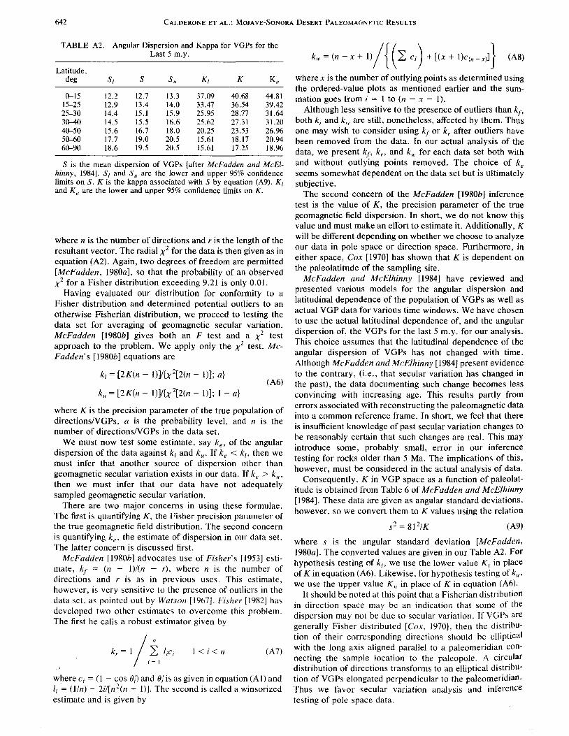
TABLE A2. Angular Dispersion and Kappa for VGPs for the Last 5 m.y.

Latitude, deg S1 s Su K1 K Ku

0-15 12.2 12.7 13.3 37.09 40.68 44.81 15-25 12.9 13.4 14.0 33.47 36.54 39.42 25-30 14.4 15.I 15.9 25.95 28.77 31.64 30-40 14.5 15.5 16.6 25.62 27.31 31.20 40-50 15.6 16.7 18.0 20.25 23.53 26.96 50-60 17.7 19.0 20.5 15.61 18.17 20.94 60-90 18.6 19.5 20.5 15.61 17.25 18.96

S is the mean dispersion of VGPs [after McFadden and McEl­~in':'y, 1984]. ~/ and S 11 are the lower and upper 95% confidence hm1ts on S. K 1s the kappa associated with S by equation (A9). K 1 and Ku are the lower and upper 95% confidence limits on K.

where n is the number of directions and r is the length of the resultant vector. The radial x2 for the data is then given as in equation (A2). Again, two degrees of freedom are permitted [McFadden, l980a], so that the probability of an observed x2 for a Fisher distribution exceeding 9.21 is only 0.01.

Having evaluated our distribution for conformity to a Fisher distribution and determined potential outliers to an otherwise Fisherian distribution, we proceed to testing the data set for averaging of geomagnetic secular variation. McFadden [1980b] gives both an F test and a x2 test approach to the problem. We apply only the x2 test. Mc­Fadden's [l980b] equations are

k1 = [2K(n - l)]l{x 2[2(n - !)]; a} (A6)

ku = [2K(n - 1)]/{x 2[2(n - !)]; I - a}

where K is the precision parameter of the true population of directions/VGPs, a is the probability level, and n is the number of directions/VGPs in the data set.

We must now test some estimate, say ke, of the angular dispersion of the data against k1 and ku. If ke < k1, then we must infer that another source of dispersion other than geomagnetic secular variation exists in our data If k > k then we must infer that our data have not. ade~uate!'; sampled geomagnetic secular variation.

There are two major concerns in using these formulae. The first is quantifying K, the Fisher precision parameter of the true geomagnetic field distribution. The second concern is quantifying ke, the estimate of dispersion in our data set. The latter concern is discussed first.

McFadden [l980b] advocates use of Fisher's [1953] esti­mate, kf = (n - l)l(n - r), where n is the number of directions and r is as in previous uses. This estimate, however, is very sensitive to the presence of outliers in the data set, as pointed out by Watson [1967]. Fisher [1982] ha~ developed two other estimates to overcome this problem. The first he calis a robust estimator given by

I< i < n (A7)

where c; = ( 1 - cos €1;) and €1/ is as given in equation (A 1) and I; = (1/n) - 2il[n 2(n + 1)]. The second is called a winsorized estimate and is given by

kw= (n - X + l) I { ( L C;) + [(x + l)c(n _ x)]} (AS)

where x is the number of outlying points as determined using the ordered-value plots as mentioned earlier and the sum­mation goes from i = 1 to (n - x - 1).

Although less sensitive to the presence of outliers than k J, both kr and kw are still, nonetheless, affected by them. Thus one may wish to consider using kf or kr after outliers have been removed from the data. In our actual analysis of the data, we present kf, k,, and kw for each data set both with and without outlying points removed. The choice of k seems somewhat dependent on the data set but is ultimate!; subjective.

The second concern of the McFadden [1980b] inference test is the value of K, the precision parameter of the true geomagnetic field dispersion. In short, we do not know this value and must make an effort to estimate it. Additionally, K will be different depending on whether we choose to analyze our data in pole space or direction space. Furthermore, in either space, Cox [1970] has shown that K is dependent on the paleolatitude of the sampling site.

McFadden and McElhinny [1984] have reviewed and presented various models for the angular dispersion and latitudinal dependence of the population of VGPs as well as actual VGP data for various time windows. We have chosen to use the actual latitudinal dependence of, and the angular dispersion of, the VGPs for the last 5 m.y. for our analysis. This choice assumes that the latitudinal dependence of the angular dispersion of VGPs has not changed with time. Although McFadden and McE/hinny [1984] present evidence to the contrary, (i.e., that secular variation has changed in the past), the data documenting such change becomes less convincing with increasing age. This results partly from errors associated with reconstructing the paleomagnetic data into a common reference frame. In short, we feel that there is insufficient knowledge of past secular variation changes to be reasonably certain that such changes are real. This may introduce some, probably small, error in our inference testing for rocks older than 5 Ma. The implications of this, however, must be considered in the actual analysis of data.

Consequently, Kin VGP space as a function of paleolat­itude is obtained from Table 6 of McFadden and McElhinny [1984]. These data are given as angular standard deviations, however, so we convert them to K values using the relation

s2 = 81 2/K (A9)

where s is the angular standard deviation [McFadden, l980a]. The converted values are given in our Table A2. For hypothesis testing of k1, we use the lower value K 1 in place of Kin equation (A6). Likewise, for hypothesis testing of ku, we use the upper value K 11 in place of K in equation (A6).

It should be noted at this point that a Fisherian distribution in direction space may be an indication that some of the dispersion may not be due to secular variation. If VGPs are generally Fisher distributed [Cox, 1970], then the distribu­tion of their corresponding directions should be elliptical with the long axis aligned parallel to a paleomeridian con­necting the sample location to the paleopole. A circular distribution of directions transforms to an elliptical distribu­tion of VGPs elongated perpendicular to the paleomeridian. Thus we favor secular variation analysis and inference testing of pole space data.

CALDERONE ET AL.: MOJAVE-SONORA DESERT PALEOMAGNETIC RESULTS 643

100

Kappa= 30 Probability level = 0.05

80

.¥: 60

40

k I

20

a~~~~~~~~~~~~~~~~~~~_.

0 5 1 0 1 5 20

N

Fig. Al. The test statistics ku and k1 of McFadden [1980b] (see equation (A6)) as a function of n for a true geomagnetic field K of 30 and a probability level, a = 0.05. Decreasing n results in a dramatic increase of ku.

In calculating statistics which estimate parameters of a true population from a small sample size, it is important to know how many "samples" are required to yield a mean­ingful estimate. McFadden [1980a] and Fisher [1982] have presented theoretical validity ranges on many statistics such as kf, k,, and kh. Based on these results, we feel that testing a data set whose number of directions/VGPs is less than five may be inappropriate on theoretical grounds alone. From our empirical observations, we furthermore believe that performing McFadden's [1980h] inference tests may yield misleading results when the number of directions/VGPs in the data set is less than 10. Figure Al shows the statistics k1 and ku as a function of N for an expected kappa value of 30. The envelope begins to increase dramatically (as it must to maintain 95% confidence) with a smaller number of samples. However, the passage of McFadden's [1980h] inference tests may, in this case, be more dependant on N than on the actual dispersion of the data. We consequently believe N < 10 is insufficient for secular variation inference testing.

In summary, we adopt the following criteria for secular variation averaging tests. We require (1) N > 10, (2) a Fisherian distribution of cooling unit VGPs, and (3) disper­sion of the VGPs should pass both McFadden's [1980h] inference tests. If outliers are present in an otherwise Fisher distribution, kr or kw is preferred over kf as the best estimate of kappa for the data set. If outliers are removed, kf or kr are generally preferred over k 11 for inference testing. We use the 95% confidence level in all of our applications of McFad­den's [1980h] tests. We prefer analysis of VGPs over direc­tions, as many workers [Cox, 1970; McFadden and McE/­hinny, 1984] have pn:sented evidence that the VGPs should be Fisher distributed. If the distribution of VGPs is not Fisherian, then sources of dispersion other than secular variation may be present, or secular variation may not actually be adequately sampled. Finally, we assume that

secular variation in the Miocene is not significantly different from that for the last 5 m. y.

Regional Cooling Unit Paleomagnetic Analysis

Ordered-value plots [Lewis and Fisher, 1982] (Figure A2) are generally linear but polluted by a few outlying points, indicating generally Fisherian distributions with a few anom­alous VGPs. Eight normal polarity outliers, three reverse polarity outliers, and five outliers in the combined polarity set were detected using this method. The distribution tests of McFadden [1980a] (see Table 4) confirm these observations. The x2 tests reveal Fisherian distributions at the 99% confidence level after outliers are removed and non­Fisherian distributions at 99% confidence with outliers present. The mean poles calculated for the data with the outliers removed are not statistically different from those calculated with outliers present at all confidence levels greater than 90%.

The normal polarity VGP data show (outliers included) more dispersion than is expected for a time-averaged data set using all k estimators except the winsorized kw. After removal of outlying normal polarity VGPs, the dispersion of these data is less than expected using any estimate of the precision parameter. In normal polarity, then, it seems that the cooling unit VGPs distributed throughout the Mojave­Sonora region do not adequately average the secular varia­tion of the geomagnetic field. It is interesting to note that the outliers all come from the Clipper Mountains. Acton [1986] suggested that the Clipper flows may have recorded an excursion or polarity transition of the geomagnetic field. This seems the most likely source of the extra dispersion in the data set without removal of these outliers.

Reverse polarity VGPs fit a Fisher distribution at 99% confidence but show more dispersion than can be accounted for by secular variation alone. Removal of outliers improves the fit to a Fisher distribution and reduces the dispersion to a level where an adequate averaging of secular variation may be accepted at 95% confidence. Again removal of the outliers does not significantly change the mean pole. The outlying VGPs of the reverse polarity data come from the Gila Bend area. These VGPs were all determined using principal com­ponent analysis, as the specimens contained a strong IRM component that masked the primary component. It is possi­ble that these mathematically determined directions are not good estimators of the geomagnetic field direction at the time they formed but rather contain some component of the secondary IRM directions. Thus the extra source of disper­sion in the VGP data for the region may be related to unremoved secondary components in the lightning-struck rocks of the Gila Bend area.

The antipode of the reverse polarity mean pole is about 8° from the normal polarity mean pole but may be accepted as statistically identical at any confidence level greater than 80o/c using the test of McFadden and Lowes [1981]. With outliers removed, the reversals test is passed at any confi­dence level greater than 90%. The angular distance between poles is again about 8°. It appears, then, that the hypothesis that the mean reverse polarity pole is antiparallel to the mean normal polarity pole cannot be rejected at confidence levels greater than 8{}-90% in spite of the small angular distance between them. It is interesting to note, however, that the discrepancy between normal and reverse polarity mean

644

IJ

u

1.3

.. O.l

I.I

u

O.I

I< .... I: 0.6 .!! • . ! ... DA .. Q

O.l r

0.0 u.o

1.0

0.5

-...

.e.s .3

A

CALDERONE ET AL.: MOJAVE-SONORA DESERT PALEOMAGNETIC RESULTS

u 0.5

• . • Normal polarity VGPs

Reverse polmity VGPs • • AllVGPs • • 1.3 0.4

• • • • • . • • • • 0.3 • O.l

• O.l • • . .. ... i .... • 0.1 . .. . .... 0.1 rl'

/ -0.0

0

E{I) E{i)

E{i)

1.0 --· •• 1.8

Normal polarity VGPs ..... Reverse polarity VGPs • • ,,

AIIVGPs ,,,,. • 0.1 . . O.I • - -• . •• O.li -0.6 .. . . • .. • .

• . • ..

~ • 0.4 . .. u _ .. ,,. ... .... '11'

• O.l ,.,,,. •• O.l • • . ·- ...

0.0 . __.

u.o 0.2 0.4 0.6 0.1 1.0 0.0 .... -0.2 0.4 0.6 0.1 1.8 u.o 0.2 0.4 0.6

U{I) U(i)

U(I)

1.8 1.0

Normal polarity VGPs Reverse polarity VGPs All VGPs •

0.5 0.5 .... .-//

.. . • • - 0.0 0.0 - ..... / •• •

• • . . .. /

.e.s .0.5

• •

.u -1.0

·2 ·1 .3 ·2 ·1 .3 -2 ·1

Q(i) B Q(i) c Q(i)

Fig. A2. Ordered-value plots of cooling unit VGP data for the entire Mojave-Sonora desert region in (a) normal polarity, (b) reversed polarity, and (c) combined polarities. Outlying points are marked with small arrows. C(i), E(i), u(i), t(i) and Q(i) are as defined by Lewis and Fisher [1982].

0.1 I.I

• •

VGPs is very similar to that reported by Diehl et al. (1988] from slightly older units in the Mogollon-Datil volcanic field. We cannot, however, eliminate the possibility that the deviation from strict antipolarity is due to insufficient aver­aging of secular variation by the normal polarity cooling units in our data rather than by a small long-term nondipole component of the geomagnetic field as suggested by Diehl et al. (1988]. Further data of global coverage would be required

to substantiate such long-term nondipole behavior of the Miocene geomagnetic field.

The combined polarity VGPs are not Fisherian at the 99% confidence level when the outliers are included. Addition­ally, the VGPs are more dispersed than can be accounted for by secular variation alone using any estimator for kappa. Removal of outlying points does not significantly alter the mean pole but results in a Fisherian distribution at 99%

CALDERONE ET AL.: MOJAVE-SONORA DESERT PALEOMAGNETIC RESULTS 645

confidence. Furthermore, the disw:rsion of VGPs with out­liers removed falls into the accepta~le range of dispersion for a study which adequately averages secular variation.

The outliers are essentially the same as described above, although several of the normal polarity outliers became "in line" with the combination of pofarities. The sources of extra dispersion are most likely the recording of a few anomalous VGPs due to magnetic excursions and incom­plete removal of lightning-induced IRM in a few additional VGPs. Excluding these few anomalous VGPs yields disper­sion similar to that expected using the 0--5 Ma geomagnetic field as a model. Thus, although other sources of dispersion such as small vertical axis rotations between ranges or improper structural corrections cannot be completely dis­counted, they are not required to account for the dispersion in the Mojave-Sonora desert. We prefer the simple explana­tion that the dispersion is simply due to geomagnetic secular variation polluted by recording a few anomalous VGPs due to magnetic field excursions and incompletely removed lightning-strike magnetizations.

Acknowledgments. We thank Cori Hoag, Nancy Johnson, Amy Ruf, Nancy Riccio, and Rich Walsh for assistance in the field and laboratory. Floyd Gray, Gordon Haxel, Dick Tosdal, Jane Nielson, and Mike Grubensky aided in the selection of sample localities and understanding of the geology of the Mojave-Sonora Desert. R. J. Miller graciously provided the K-Ar data for the White Hills. We have benefitted from numerous discussions with Peter Coney, Clem Chase, Steve Reynolds, Terry Wallace, Randy Richardson, Monte Marshall, and Joe Butterworth. Steve Sorenson rescued us from the depths of FORTRAN many times. Norm Meader provided invalu­able word processing assistance. Thoughtful reviews by Hugh Rieck, Jonathan Hagstrom, Bruce Luyendyk, and Jack Hillhouse led to a much improved manuscript. Funding for this project was provided by the National Science Foundation (EAR-8617240) and the U.S. Geological Survey.

REFERENCES

Acton, G. D., Paleomagnetism of Miocene volcanic rocks in the Mojave region of southeastern California, M.S. thesis, 73 pp., Univ. of Ariz., Tucson, 1986.

Aldridge, M. J., and A. W. Laughlin, The Sonoran Desert tectono­physical subprovince, Geo/. Soc. Am. Abstr. Programs, 15, 315, 1983.

Alvarez, W., D. V. Kent, I. Silva, R. Schweikert, and R. Larson, Franciscan complex limestone deposited at 17° south paleolati­tude, Geo/. Soc. Am. Bull., 91, 476-484, 1980.

Atwater, T., Implications of plate tectonics for the tectonic evolu­tion of western North America, Geo/. Soc. Am. Bull., 81, 3513-3536, 1970.

Barnes, A. E., and R. F. Butler, A Paleocene paleomagnetic pole from the Gringo Gulch volcanics, Geophys. Res. Lett., 7, 545-548, 1980.

Bates, R. G., M. E. Beck, Jr., and R. Burmester, Tectonic rotations in the Cascade Range of southern Washington, Geology. 9. 184-189, 1981.

Beck, M. E., Jr., Discordant paleomagnetic pole positions as evidence of regional shear in the western Cordillera of North America, Am. J. Sci., 276, 694-712. 1976.

Beck, M. E., Jr., Paleomagnetic record of plate margin processes along the western edge of North America, J. Geophys. Res .. 85. 7115-7131, 1980.

Best, M. G., E. H. McKee, and P. E. Damon, Space-time­composition patterns of late Cenozoic mafic volcanism, south­western Utah and adjoining areas, Am. J. Sci., 280, 1035-1050, 1980.

Bryan, P., and R. G. Gordon, Rotation of the Colorado Plateau: an analysis ofpaleomagnetic data, Tecto~ics, 5, 661-{;67, 1986.

Burchfiel, B. C., and G. A. Davis, Mojave Desert environs, in The Geotectonic Development of California, Ru bey Volume 1, edited

by W. G. Ernst, pp. 218-252, Prentice-Hall, Englewood Cliffs, N. J., 1981.

Burke, D. B., J. W. Hillhouse, E. H. McKee, S. T. Miller, and J. L. Morton, Cenozoic rocks in the Barstow Basin area of southern California-Stratigraphic relations, radiometric ages, and paleo­magnetism, U.S. Geo/. Surv. Bull., 1529-E, 1-16, 1982.

Butterworth, J., Paleomagnetic investigation of mid-Tertiary vol­canic rocks in the Castle Dome and southern Kofa Mountains, Yuma County, Arizona, M.S. thesis, 195 pp., San Diego State Univ., San Diego, Calif., 1984.

Calderone, G. J., Paleomagnetism of Miocene volcanic rocks in the Mojave-Sonora desert region of western Arizona and southeast­ern California, Ph.D. thesis, 163 pp., Univ. of Ariz., Tucson, 1988.

Calderone, G., and R. F. Butler, Paleomagnetism of Miocene volcanic rocks from southwestern Arizona: Tectonic implica­tions, Geology, 12, 627-{;30, 1984.

Callian, J. T., A paleomagnetic study of Miocene volcanics from the Colorado River and mainland Mexico regions, M.S. thesis, 111 pp., San Diego State Univ., San Diego, Calif., 1984.

Carter, J. N., B. P. Luyendyk, and R.R. Terres, Neogene clock­wise tectonic rotation of the eastern Transverse Ranges, Califor­nia, suggested by paleomagnetic vectors, Geo/. Soc. Am. Bull., 98, 199-206, 1987.

Champion, D. E., D. G. Howell, and C. S. Gromme, Paleomagnetic and geologic data indicating 2500 km of northward displacement for the Santa Lucia-Orocopia allocthon, J. Geophys. Res., 89, 7736-7752, 1984.

Christiansen, R. L., and P. W. Lipman, Cenozoic volcanism and plate tectonic evolution of the western United States, 2, Late Cenozoic, Philos. Trans. R. Soc. London, 271, 249--284, 1972.

Coney, P. J., Mesozoic-Cenozoic Cordilleran plate tectonics, Cen­ozoic Tectonics and Regional Geophysics of the Western Cordil­lera, Mern. Geo/. Soc. Am., 152, 33-50, 1978.

Coney, P. J., and S. J. Reynolds, Cordilleran Benioffzones, Nature, 270, 403-406, 1977.

Coney, P. J .. D. L. Jones, and J. W. Monger, Cordilleran suspect terranes, Nature, 288, 329-333, 1980.

Costello, S. C., A paleomagnetic investigation of mid-Tertiary volcanic rocks in the lower Colorado River area, M.S. thesis, 109 pp., San Diego State Univ., San Diego, Calif., 1985.

Cox, A., Latitude dependence of angular dispersion of the geomag­netic field, Geophys. J. R. Astron. Soc., 20, 253-269, 1970.

Cox, A., and R. G. Gordon, Paleolatitudes determined from vertical cores, Rev. Geophys., 22, 47-72, 1984.

Davis, G. A., J. L. Anderson, D. L. Martin, D. Krummenacher, E. G. Frost, and R. L. Armstrong, Geologic and geochronologic relations in the lower plate of the Whipple detachment fault, in Mesozoic-Cenozoic Tectonic Evolution of the Colorado River Region, California, Arizona, and Nevada, edited by E. G. Frost and D. M. Martin, pp. 408-432, Cordilleran Publishers, San Diego, Calif., 1982.

Dickinson, W. R., Plate tectonic evolution of the Southern Cordil­lera, Relations of Tectonics to Ore Deposits in the Southern Cordillera, Ariz. Geo/. Soc. Dig., 14, 113-135, 1981.

Diehl, J. F., K. M. McColannahan, and T. J. Bornhorst, Paleomag­netic results from the Mogollon-Datil volcanic field, southwestern New Mexico, and a refined Mid-Tertiary reference pole for North America, J. Geophys. Res., 93, 4869-4879, 1988.

Dokka, R. K., Displacement on late Cenozoic strike-slip faults of the central Mojave desert, California, Geology, 11, 305-308, 1983.

Eberly, L. D., and T. B. Stanley. Jr., Cenozoic stratigraphy and geologic history southwestern Arizona, Geo/. Soc. Arn. Bull., 89, 921-940, 1978.

Fisher, N. I.. Robust estimation of the concentration parameter of Fisher distribution on a sphere, Appl. Stat., 31, 152-154, 1982.

Fisher, N. I., T. Lewis, and B. J. J. Embleton, Statistical Analysis of Spherical Data, 329 pp., Cambridge University Press, New York, 1987.

Fisher, R. A., Dispersion on a sphere, Proc. R. Soc. London, Ser. A. 217, 295-305, 1953.

Garfunkel, Z., Model for the late Cenozoic history of the Mojave desert, California, and for its relation to adjacent regions, Geo/. Soc. Arn. Bull., 85, 1931-1944, 1974.

Geissman. J. W., Paleomagnetism and Late Cenozoic strike-slip tectonism in the Hoover Dam area. southeast extension of the

646 CALDERONE ET AL.: MOJAVE-SONORA DESERT PALEOMAGNETIC RESULTS

Lake Mead fault zone, Nevada and Arizona (abstract), Eos Trans. AGU, 67, 922, 1986.

Glazner, A. F., J. E. Nielson, K. A. Howard, and D. M. Miller, Correlation of the Peach Springs Tuff, a large-volume Miocene ignimbrite sheet in California and Arizona, Geology, 14, 840-844, 1986.

Golombek, M. P., and L. L. Brown, Clockwise rotation of the western Mojave Desert, Geology, 16, 126-129, 1988.

Gray, F., and R. S. Miller, New K-Ar ages of volcanic rocks near Ajo, Pima and Maricopa counties, southwestern Arizona, /so­chron West, 41, 3-6, 1984.

Gromme, C. S., M. E. Beck, Jr., R. E. Wells, and D. C. Engebret­son, Paleomagnetism of the Tertiary Clarno Formation of central Oregon and its significance for the tectonic history of the Pacific northwest, J. Geophys. Res., 91, 14,089-14, 104, 1986.

Hagstrom, J. T., M. 0. McWilliams, D. G. Howell, and C. S. Gromme, Mesozoic paleomagnetism and northward translation of the Baja California peninsula, Geo/. Soc. Am. Bull., 96, 1077-1090, 1985.

Hagstrom, J. T., D. P. Cox, and R. J. Miller, Structural reinterpre­tation of the Ajo Mining District, Pima County, Arizona, based on paleomagnetic and geochronologic studies, Econ. Geo/., 82, 1348-1361, 1987a.

Hagstrom, J. T., M. G. Sawlan, B. P. Hausback, J. G. Smith, and C. S. Gromme, Miocene paleomagnetism and tectonic setting of the Baja California peninsula, Mexico, J. Geophys. Res., 92, 2627-2640, 1987b.

Halls, H. C., A least-squares method to find a remanence direction from converging remagnetization circles, Geophys. J. R. Astron. Soc., 45, 297-304, 1976.

Hamilton, W., Plate-tectonic mechanism of Laramide deformation, Contrib. Geo/., 19, 87-92, 1981.

Harrison, C. G. A., and T. Lindh, A polar wandering curve for North America during the Mesozoic and Cenozoic, J. Geophys. Res., 87, 1903-1920, 1982.

Hillhouse, J. W., Paleomagnetism of the Triassic Nikolai Green­stone, McCarthy Quadrangle, Alaska, Can. J. Earth Sci., 14, 2578-2592, 1977.

Hillhouse, J. W., and C. S. Gromme, Northward displacement and accretion of Wrangellia: New paleomagnetic evidence from Alaska, J. Geophys. Res., 89, 4461-4477, 1984.

Hillhouse, J. W., and M. 0. McWilliams, Application ofpaleomag­netism to accretionary tectonics and structural geology, Rev. Geophys., 25, 951-959, 1987.

Hillhouse, J. W., and R. E. Wells, Assessment of rotations in the Eastern Mojave Desert, California and Arizona, from Paleomag­netism of the Peach Springs Tuff (abstract), Eos Trans. AGU, 67, 922, 1986.

Hoffman, K. A., and R. Day, Separation of multicomponent NRM: A general method, Earth Planet. Sci. Lett., 40, 433-438, 1978.

Hornafius, J. S., B. P. Luyendyk, R.R. Terres, and M. 1. Kamer­ling, Timing and extent of Neogene tectonic rotation in the western Transverse Ranges, California, Geo/. Soc. Am. Bull., 97, 1476-1487, 1986.

Irving, E., Paleopoles and paleolatitudes of North America and speculations about displaced terranes, Can. J. Earth Sci., 16, 669-694, 1979.

Irving, E., and G. A. Irving, Apparent polar wander paths, Car­boniferous through Cenozoic and the assembly of Gondwana, Geophys. Surv., 5, 141-188, 1982.

Kamerling, M., and B. Luyendyk, Tectonic rotations of the Santa Monica mountains region, western Transverse Ran11es, Califor­nia, suggested by paleomagnetic vectors, Geo/. Soc. Am. Bull .. 90. 33!-337. 1979.

Kamerling, M. J., and B. P. Luyendyk. Paleomagnetism and Neo­gene tectonics of the Northern Channel Islands, California, J. Geophys. Res., 90, 12,485-12,502, 1985.

Kirschvink, J. L., The least-squares line and plane and the analysis ofpaleomagnetic data, Geophys. J. R. Astron. Soc., 62, 699-718, 1980. '

Kluth, C. F., R. F. Butler, L. E. Harding, M. Shafiqullah, and P. E. Damon; Paleomagnetism of late Jurassic rocks in the northern Canelo Hills, southeastern Arizona, J. Geophys. Res., 87, 7078-7086, 1982.

Lewis, T., and N. I. Fisher, Graphical methods for investigating the

fit of a Fisher distribution for spherical data, Geophys. J. R. Astron. Soc., 69, 1-13, 1982.

Luedke, R. G., and R. L. Smith, Map showing distribution, com­position and age of late Cenozoic volcanic centers in Arizona and N. Mexico, U.S. Geo/. Surv. Misc. Invest. Map, 1-1091-a, 1978.

Luyendyk, B. P., M. J. Kamerling, and R. R. Terres, Geometric model for Neogene crustal rotations in southern California, Geo/. Soc. Am. Bull., 91, 211-217, 1980.

Luyendyk, B. P., M. J. Kamerling, R. R. Terres, and J. S. Hornafius, Simple shear of southern California during Neogene time suggested by paleomagnetic declinations, J. Geophys. Res., 90, 12,454-12,466, 1985.

MacFadden, B. J., M. 0. Woodburne, and N. D. Opdyke, Paleo­magnetism and Neogene clockwise rotation of the northern Cady Mountains, Mojave Desert of sourthern California, J. Geophys. Res., in press, 1990.

Magill, J., and A. Cox, Post-Oligocene tectonic rotation of the Oregon western Cascade Range and the Klamath Mountains, Geology, 9, 127-131, 1981.

Magill, J., A. Cox, and R. Duncan, Tillamook volcanic series: Further evidence for tectonic rotation of the Oregon Coast Range, J. Geophys. Res., 86, 2953-2970, 1981.

Mankinen, E. A., E. E. Larson, C. S. Gromme, M. Prevot, and R. S. Coe, The Steens Mountain (Oregon) geomagnetic polarity transition, 3, Its regional significance, J. Geophys. Res., 92, 8057-8076, 1987.

May, S. R., P. J. Coney, and M. E. Beck, Jr., Paleomagnetism and suspect terranes of the North American Cordillera, U.S. Geo/. Surv. Open File Rep., 83-799, 8 pp., 1983.

May, S. R., R. F. Butler, M. Shafiqullah, and P. E. Damon, Paleomagnetism of Jurassic volcanic rocks in the Patagonia Mountains, southeastern Arizona: Implications for the North American 170 Ma reference pole, J. Geophys. Res., 91, 11,545-11,555, 1986.

McCurry, M. 0., Evolution of the Woods Mountain volcanic center, eastern Mojave Desert, Geo/. Soc. Am. Abstr. Programs, 18, 156, 1986.

McFadden, P. L., The best estimate of Fisher's precision parameter K, Geophys. J. R. Astron. Soc., 60, 397-407, 1980a.

McFadden, P. L., Testing a paleomagnetic study for the averaging of secular variation, Geophys. J. R. Astron. Soc., 61, 183-192, 1980b.

McFadden, P. L., and F. J. Lowes, The discrimination of mean directions drawn from Fisher distributions, Geophys. J. R. As­tron. Soc., 67, 19-33, 1981.

McFadden, P. L., and M. W. McElhinny, A physical model for paleosecular variation, Geophys. J. R. Astron. Soc., 78, 809-830, 1984.

McFadden, P. L., and A. B. Reid, Analysis of paleomagnetic inclination data, Geophys. J. R. Astron. Soc., 69, 307-319, 1982.

McWilliams, M. 0., Paleomagnetism and the motion of large and small plates, Rev. Geophys., 21, 644-651, 1983.

McWilliams, M. 0., Confidence limits on net tectonic rotation, Geophys. Res. Lett., II, 825-827, 1984.

Morris, L. K., S. P. Lund, and D. J. Bottjer, Paleolatitude drift history of displaced terranes in southern and Baja California, Nature, 321, 844-847, 1986.

Percious, J. K., Geology and geochronology of the Del Bae Hills, Pima county, Arizona, in Southern Arizona Guidebook /II, edited by S. R. Tilley, pp. 199-207, Arizona Geological Society, Tucson, 1968.

Ross, T. M., B. P. Luyendyk, and R. B. Naston, Paleomagnetic evidence for Neogene tectonic rotations in the central Mojave desert. California. Geo/. Soc. Am. Ahstr. Programs .. 20. 226. 1988.

Ross, T. M .. B. P. Luyendyk, and R. B. Naston. Paleomagnetic evidence for Neogene clockwise tectonic rotations in the central Mojave Desert, California, Geology, 17, 470-473, 1989.

Sass, J. H., and A.H. Lachenbruch, Heat-flow field of the Califor­nia-Arizona crustal experiment and adjacent areas, Geo/. Soc. Am. Ahstr. Programs, 19, 829, 1987.

Shafiqullah, M., P. E. Damon, D. J. Lynch, S. J. Reynolds, W. A. Rehrig, and R. H. Raymond, K-Ar geochronology and geologic history of southwestern Arizona and adjacent areas, Studies in Western Arizona, Ariz. Geo/. Soc. Dig., 12, 201-260, 1980. '

CALDERONE ET AL.: MOJAVE-SONORA DESERT PALEOMAGNETIC RESULTS 647

Simpson, R. W., and A. Cox, Paleomllgnetic evidence for tectonic rotation in the Oregon Coast Range,-Geo/ogy, 5, 585-589, 1977.

Spencer, J. E., Miocene low-angle normal faulting and dike em­placement, Horner Mountain and surrounding areas, southeastern California and southernmost Nevada, Geo/. Soc. Am. Bull., 96, 1140--1155, 1985.

Spencer, J. E., and S. J. Reynolds, Some aspects of the Middle Tertiary tectonics of Arizona and southeastern California, Fron­tiers in Geology and Ore Deposits of Arizona and the Southwest, Ariz. Geo/. Soc. Dig., 16, 102-107, 1986.

Stewart, J. H., Basin and Range structure in western North Amer­ica: A review, Cenozoic Tectonics and Regional Geophysics of the Western Cordillera, Mem. Geo/. Soc. Am., 152, 1-31, 1978.

Symons, D. T. A., and M. Stupavsky, A rational paleomagnetic stability index, J. Geophys. Res., 79, 1718-1720, 1974.

Thompson, G. A., and D. B. Burke, Regional Geophysics of the Basin and Range province, Annu. Rev. Earth Planet. Sci., 2, 213-238, 1973.

Veseth, M., Paleomagnetism of the Kofa Mountains, southwestern Arizona, and implications for mid-Tertiary and younger extension in the Basin and Range province, M.S. thesis, 123 pp., San Diego State Univ., San Diego, Calif., 1985.

Veseth, M., J. Butterworth, and M. Marshall, A paleomagnetic investigation of Miocene volcanic rocks, Yuma County, south­west Arizona (abstract), Eos Trans. AGU, 63, 913, 1982.

Vugtaveen, R. W., A. E. Barnes, and R. F. Butler, Paleomagnetism of the Roskruge and Gringo Gulch volcanics, southeast Arizona, J. Geophys. Res., 86, 4021-4028, 1981.

Watson, G. S., Analysis of dispersion on a sphere, Mon. Not. R. Astron. Soc., 7, 153-161, 1956.

Watson, G. S., Some problems in the statistics of directions, Bull. 36th Session, Int. Stat. Inst., Sydney, Australia, 1967.

Wells, R. E., and P. L. Heller, The relative contribution of accre­tion, shear, and extension to Cenozoic tectonic rotation in the Pacific Northwest, Geo/. Soc. Am. Bull., JOO, 325-338, 1988.

Wells, R. E., and J. W. Hillhouse, Tectonic rotations in the Peach Springs Tuff, Colorado River extensional corridor, California and Arizona, Geo/. Soc. Am. Abstr. Programs, 19, 886, 1987.

Wells, R. E., and J. W. Hillhouse, Paleomagnetism and tectonic rotation of the lower Miocene Peach Springs Tuff-Colorado Plateau, Arizona to Barstow, California, Geo/. Soc. Am. Bull., JOI, 846-863, 1989.

Wesnousky, S. G., Earthquakes, Quaternary faults and seismic hazard in California, J. Geophys. Res., 91, 12,587-12,632, 1986.

G. D. Acton, Department of Geological Sciences, Northwestern University, Evanston, IL 60201.

R. F. Butler, Department of Geosciences, University of Arizona, Tucson, AZ 85721.

G. J. Calderone, U.S. Geological Survey, 2255 North Gemini Drive, Flagstaff, AZ 86001.

(Received March 2, 1989; revised August 30, 1989; accepted May 21, 1989.)