Exciton condensation in strongly correlated electron bilayers

Louk Rademaker,1, ∗ Jeroen van den Brink,2, 3 Jan Zaanen,1 and Hans Hilgenkamp1, 4

1Institute-Lorentz for Theoretical Physics, Leiden University, PO Box 9506, Leiden, The Netherlands2Institute for Theoretical Solid State Physics, IFW Dresden, 01171 Dresden, Germany

3Department of Physics, TU Dresden, D-01062 Dresden, Germany4Faculty of Science and Technology and MESA+ Institute for Nanotechnology,University of Twente, P.O. Box 217, 7500 AE Enschede, The Netherlands

(Dated: October 31, 2018)

We studied the possibility of exciton condensation in Mott insulating bilayers. In these stronglycorrelated systems an exciton is the bound state of a double occupied and empty site. In the strongcoupling limit the exciton acts as a hard-core boson. Its physics are captured by the exciton t− Jmodel, containing an effective XXZ model describing the exciton dynamics only. Using numericalsimulations and analytical mean field theory we constructed the ground state phase diagram. Threehomogeneous phases can be distinguished: the antiferromagnet, the exciton checkerboard crystaland the exciton superfluid. For most model parameters, however, we predict macroscopic phaseseparation between these phases. The exciton superfluid exists only for large exciton hoppingenergy. Additionally we studied the collective modes and susceptibilities of the three phases. Inthe superfluid phase we find the striking feature that the bandwidth of the spin-triplet excitations,potentially detectable by resonant inelastic x-ray scattering (RIXS), is proportional to the superfluiddensity. The superfluid phase mode is visible in the charge susceptibility, measurable by RIXS orelectron energy loss spectroscopy (EELS).

PACS numbers: 71.35.Lk, 71.27.+a, 73.20.Mf

I. INTRODUCTION

Strongly correlated electron systems exhibit the high-est attained superconducting transition temperaturescurrently known, and a rich variety of complex elec-tronic phases1,2. Many compounds among this familyof Mott insulators, such as the cuprates, are quasi-two-dimensional layered materials. This renders them idealcandidates for bilayer exciton condensation, which is thetopic of this publication.

The effort to achieve the condensation of excitons hasa long history starting just after the discovery of BCStheory3–5. An exciton is the bound state of an electronand a hole and as such it can Bose condense. The obviousadvantage of considering excitons above Cooper pairs isthe strong Coulomb attraction between the electron andthe hole; allowing in principle for a much higher criticaltemperature. To reduce the exciton lifetime problemscaused by electron-hole recombination, it has been sug-gested to spatially separate the electrons and holes intheir own subsequent layers6,7. This indeed has resultedin the experimental realization of exciton condensates,first in the so-called quantum Hall bilayers8 and morerecently without an externally applied magnetic field inelectrically gated, optically pumped semiconductor quan-tum wells9.

The successes of exciton condensation in semiconduc-tor 2DEG bilayer systems have led to many proposalsfor exciton condensation in alternative bilayer materi-als, such as gated topological insulators10 or double layergraphene11–15. However, these proposals are limited tothe BCS paradigm of weak coupling.

On the other hand, Mott insulators provide a com-

Exciton

FIG. 1: Side view of a strongly correlated electron bilayerwith an exciton present. The red arrows denote the spin ofthe localized electrons, and the exciton is a bound state of adouble occupied and an empty site.

pletely different route to exciton condensation16–18.Naively one would expect that the localization of theelectrons and holes leads to a higher critical tempera-ture, since Tc is determined by the competition betweenthe electronic kinetic energy and the electron-hole attrac-tion. But the physics of exciton condensation in Mottinsulators is in fact much richer.

Instead of the picture that the electron-hole pair livesin a conduction and valence band, an exciton now con-sists of a double occupied and vacant site bound togetheron an interlayer rung, see figure 1. To estimate the bind-ing energy, consider the in-plane charge-transfer excitonswhich are known to have a binding energy of the orderof 1-2 eV19. Due to the small interlayer distances of or-der 1 nm we expect that a similar energy scale will setthe binding of the interlayer exciton. As such, excitonsin a Mott bilayer are most likely in the strongly coupledregime.

Furthermore, a single doublon-holon pair insertedinto a Mott insulator leads to dynamical frustration

arX

iv:1

310.

0685

v1 [

cond

-mat

.str

-el]

2 O

ct 2

013

2

effects20,21, even stronger than seen for a single hole inthe t − J model23,24. The study of excitons in stronglycorrelated materials thus catches the complexity of dopedMott insulators. As we discussed elsewhere21 the bosonicnature of the excitons actually falls short to completelyeliminate all ”fermion-like” signs: there are still left-oversigns of the phase-string type22. However, it is easy todemonstrate that collinear spin order is a sufficient condi-tion for these signs to cancel out, leaving a truly bosonicdynamics controlling the ground state and long wave-length physics. The problem thereby reduces to that ofhard-core bosons (the excitons) in a sign-free spin back-ground. This is very similar to the ”spin-orbital” physicsdescribed by Kugel-Khomskii type models25, which canbe viewed after all as describing d-d excitons interact-ing with spins. Also the lattice implementations26 of theSO(5) model27 for (cuprate) superconductivity are in thisfamily.

Such bosonic problems can be handled with stan-dard (semi-classical) mean field theory, and therefore theregime of finite exciton density can be addressed in ana-priori controlled manner. In most bilayer exciton set-ups, such as the quantum Hall bilayers or the pumpedsystems, there is no controllable equilibrium exciton den-sity. In these cases one can hardly speak of the excitondensity as a conserved quantity, and exciton condensa-tion in the sense of spontaneously broken U(1) symmetryis impossible28. However, in Mott insulators the dopantdensity per layer could be fixed by, for example, chemicaldoping. The effective exciton chemical potential is thenby definition large compared to the recombination rate.Effectively, the excitons are at finite density in equilib-rium and hence spontaneous U(1) symmetry breaking ispossible in the Mott insulating bilayer.

Besides the exciton superfluid phase one anticipates aplethora of competing orders, as is customary in stronglycorrelated materials. At zero exciton density the bi-layer Heisenberg system exhibits already interesting mag-netism, in the form of the antiferromagnet for small rungcoupling turning via an O(3)-QNLS quantum phase tran-sition into an ”incompressible quantum spin liquid” forlarger rung couplings that can be viewed as a continu-ation of pair singlets (”valence bonds”) stacked on therungs29. The natural competitor of the exciton super-fluid at finite density is the exciton crystal and one an-ticipates that due to the strong lattice potential this willtend to lock in at commensurate densities forming ex-citon ”Mott insulators”. We will wire this in by tak-ing also the exciton-exciton dipolar interaction into ac-count that surely promotes such orderings. In principlethere is the interesting possibility that all these ordersmay coexist microscopically forming an ”antiferromag-netic supersolid”30. In this bosonic setting we can ad-dress it in a quite controlled manner, but we find that atleast for the strongly coupled ”small” excitons assumedhere this does not happen. The reason is interesting. Wealready alluded to the dynamical ”frustration” associatedwith the exciton delocalizing in the anti-ferromagnetic

spin background, which is qualitatively of the same kindas for the standard ”electron” t-J model. At finite densi-ties this turns into a tendency to just phase separate ona macroscopic scale, involving antiferromagnets, excitoncrystalline states and high density diamagnetic excitonsuperfluids, respectively.

Even though the exciton dipolar repulsion is long-ranged, there is no possibility of frustrated phase separa-tion as suggested for the electronic order in cuprates31–35

because the 1/r3 interaction falls off too quickly. How-ever, if one correctly incorporates the full exciton dipolarinteraction, a variety of different exciton ordered phasemay arise36. Here we restrict ourselves to nearest neigh-bor repulsion only, which allows for the formation of acheckerboard ordered exciton crystalline state.

It is disappointing that apparently in this system onlyconventional ground states occur. However, this is ac-tually to a degree deceptive. The Hamiltonian describ-ing the physics at the lattice scale describes a physicswhere the exciton- and spin motions are ”entangled”:the way in which these subsystems communicate gets be-yond the notion of just being strongly coupled, since themotions of the exciton motions and the spin dynamicscannot be separated. By coarse graining this all the wayto the static order parameters (the mean fields) an ef-fective decoupling eventually results as demonstrated bythe pure ground states. However, upon going ”off-shell”this spin-exciton entanglement becomes directly mani-fest in the form of unexpected and rather counterintu-itive effects on the excitation spectrum. A simple ex-ample is the zero exciton density antiferromagnet. Fromthe rather controlled linear spin wave self-consistent Bornapproximation (LSW-SCBA) treatment of the one exci-ton problem20 we already know that the resulting excitonspectrum can be completely different from that in a sim-ple semiconductor. We compute here the linearized exci-tations around the pure antiferromagnet, recovering theLSW-SCBA result in the ”adiabatic limit” where the ex-citon hopping is small compared to the exchange energyof the spin system, which leads to a strong enhancementof the exciton mass. In the opposite limit of fast excitons,the energy scale is recovered but the ”Ising-confinement”ladder spectrum revealed by the LSW-SCBA treatment isabsent. The reason is clear: in the language of this paper,the couplings between the exciton- and spin-wave modesbecome very big and these need to be re-summed in orderto arrive at an accurate description of the exciton prop-agator, while our mean-field treatment corresponds witha complete neglect of these exciton-spin interactions.

The real novelty in this regard is revealed in the highdensity exciton superfluid phase. The spin system formshere a ground state that is a product state of pair-singletsliving on the rungs. Besides the superfluid phase modesone expects in addition also the usual massive spin-tripletexcitations associated with the (incompressible) singletvacuum. The surprise is that these are characterized bya dispersion which is in part determined by the super-fluid density of the exciton condensate, as we already an-

3

nounced elsewhere37 for which we present here the de-tails. Counterintuitively, by measuring the spin fluctua-tions one can in principle determine whether the excitonsare condensed in a superfluid.

Let us complete this introduction by specifying thepoint of departure: the Hamiltonian describing stronglybound excitons propagating through a bilayer Heisenbergspin 1/2 system. This model is derived and discussed atlength in our earlier papers20,21 and here we just sum-marize the outcome. Due to the strong electron-electroninteractions the electronic degrees of freedom are, at elec-tronic half-filling, reduced to spin operators sil governedby the bilayer Heisenberg model29,38

HJ = J∑〈ij〉,l

sil · sjl + J⊥∑i

si1 · si2. (1)

The subscript denotes spin operators on site i in layerl = 1, 2. The Heisenberg HJ is antiferromagnetic withJ > 0 and J⊥ > 0. The interlayer exciton can hoparound, thereby interchanging places with the spin back-ground. In the strong-coupling limit of exciton bindingenergies the exciton hopping process is described by theHamiltonian

Ht = −t∑〈ij〉

|Ej〉

(|0 0〉i〈0 0|j +

∑m

|1 m〉i〈1 m|j

)〈Ei|.

(2)where |E〉 is the exciton state on an interlayer rung, and|s m〉 represent the rung spin states. Whenever an exci-ton hops, it effectively exchanges the spin configurationon its neighboring site. This exciton t − J model wasderived earlier in Refs.20,21, where the optical absorptionwas computed in the limit of vanishing exciton density〈|E〉〈E|〉 → 0. In order to study the system with a finitedensity of excitons, we need to enrich the current t − Jmodel with two extra terms: a chemical potential and anexciton-exciton interaction.

The chemical potential is straightforwardly

Hµ = −µ∑i

|Ei〉〈Ei|. (3)

The exciton-exciton interaction requires more thought.The bare interaction between two interlayer excitonsresults from their electric dipole moment. Since allinterlayer exciton dipole moments are pointing in thesame direction the full exciton-exciton interaction is de-scribed by a repulsive 1/r3 interaction. Hence the in-teraction strength decays sufficiently fast to avoid theCoulomb catastrophe responsible for frustrated phaseseparation32,33. We consider it reasonable to only includethe nearest-neighbor repulsion,

HV = V∑〈ij〉

(|Ei〉〈Ei|) (|Ej〉〈Ej |) . (4)

Here V is the energy scale associated with nearest neigh-bor exciton repulsion. This number can get quite high:

given a typical interlayer distance1 of 8A and an inter-site distance of 4A the bare dipole interaction energy is14 eV. In reality, we expect this energy to be lower dueto quantum corrections and screening effects. However,the exciton-exciton interaction scale remains on the or-der of electronvolts and thus larger than the estimatedHeisenberg J and hopping t.

Let us finally consider the effects of interlayer hoppingof electrons, which leads to the annihilation of excitons,

Ht⊥ = −t⊥∑i

|Ei〉〈0 0|i + h.c. (5)

This term explicitly breaks the U(1) symmetry associ-ated with the conservation of excitons. While this termis almost certainly present in any realistic system, it is amatter of numbers whether it is relevant. In the presentcase of cuprates, where each layer can be doped by meansof chemical substitution, we expect the chemical poten-tial µ to be significantly larger than the interlayer tun-neling t⊥. Consequently, the interlayer hopping is barelyrelevant. Throughout this publication we will discuss theeffects that the inclusion of a small t⊥ will have.

The full model Hamiltonian describing a finite densityof excitons in a strongly correlated bilayer is thus

H = HJ +Ht +Hµ +HV . (6)

Let us now summarize the layout of our paper. Mostof the physics of hard-core excitons on a lattice can becaptured using an effective XXZ model, which is studiedin section II. The ground state phase diagram of the fullexciton t − J model is derived in section III, using bothnumerical simulations and analytical mean field theory.The excitations and the corresponding susceptibilities arediscussed in section IV. We conclude this paper with adiscussion on possible further lines of theoretical and ex-perimental research in section V.

II. AN EFFECTIVE XXZ MODEL

The Hamiltonian, equation (6), has five model param-eters: J , J⊥, t, V and µ. However, most properties of theexcitons can be understood by considering the problem ofhard-core bosons on a lattice. In this section we will ar-gue that the exciton degrees of freedom can be describedby an effective XXZ model. Based on some reflectionson the mathematical symmetries of the full exciton t−Jmodel, we will describe the properties of this effectiveXXZ model in subsection II B. We will conclude thissection with an outline of the method used to obtain theexcitation spectrum of the model.

A. Dynamical and symmetry algebra

Before characterizing different phases of the model weneed to assess the algebraic structure of the exciton t−J

4

model. The set of all operators that act on the localHilbert space form the dynamical algebra, whereas thesymmetries of the system are grouped together in thesymmetry algebra.

To derive the dynamical algebra, it is instructive tostart with the bilayer Heisenberg model which has, oneach interlayer rung, a SO(4) ∼= SU(2)×SU(2) dynami-cal algebra39. Upon inclusion of the exciton hopping termwe need more operators, since now the local Hilbert spaceon an interlayer rung is five-dimensional (four spin statesand the exciton). Consider the spin-to-exciton operatorE+sm ≡ |E〉〈s m| and its conjugate E−sm = (E+

sm)†. Theircommutator reads

[E+sm, E

−sm] = |E〉〈E| − |s m〉〈s m| ≡ 2Ezsm (7)

where we have introduced the operator Ezsm to completea SU(2) algebraic structure. We could set up such aconstruction for each of the four spin states |s m〉. Underthese definitions the exciton hopping term, equation (2),can be rewritten in terms of an XY -model for each spinstate,

Ht = −t∑

<ij>,sm

(E+sm,iE

−sm,j + E−sm,iE

+sm,j

)(8)

= −2t∑

<ij>,sm

(Exsm,iE

xsm,j + Eysm,iE

ysm,j

)(9)

where the sum over sm runs over the singlet and the threetriplets. Note that the exciton chemical potential, equa-tion (3), acts as an externally applied magnetic field tothis XY -model, and that the exciton-exciton repulsion,equation (4), can be rewritten as an antiferromagneticIsing term in the Ezsm operators. The dynamical algebratherefore contains four SU(2) algebras in addition to theSO(4) from the bilayer Heisenberg part. The closure ofsuch an algebra is necessarily SU(5), which is the largestalgebra possible acting on the five-dimensional Hilbertspace. Hence we need a full SU(5) dynamical algebra todescribe the exciton t − J model at finite density. Theoperators that compose this algebra are enumerated inAppendix A.

From the XY -representation of the hopping term onecan already deduce that we have four distinct U(1) sym-metries associated with spin-exciton exchange. The bi-layer Heisenberg model contains two separate SU(2)symmetries, associated with in-phase and out-phase in-terlayer magnetic order. Therefore the full symmetryalgebra of the model is [SU(2)]2 × [U(1)]4.

Breaking of the SU(2) symmetry amounts to mag-netic ordering, which is most likely antiferromagnetic(and therefore also amounts to a breaking of the latticesymmetry). Each of the U(1) algebras can be brokenleading to exciton condensation. Note that next to possi-ble broken continuous symmetries, there also might existphases with broken translation symmetry. The checker-board phase, already anticipated in the introduction, isan example of a phase where the lattice symmetry is bro-ken into two sublattices.

B. What to expect: an effective XXZ model

When discussing the dynamical algebra of the excitont−J model we found that the exciton hopping terms aresimilar to an XY -model. The main reason is that the ex-citons are, in fact, hard-core bosons and thus allow for amapping onto pseudospin degrees of freedom. Viewed assuch, the exciton-exciton interaction equation (4) is sim-ilar to an antiferromagnetic Ising term and the excitonchemical potential equation (3) amounts to an externalmagnetic field in the z-direction. Together they form anXXZ-model in the presence of an external field, whichhas been investigated in quite some detail elsewhere40–45

as well as in the context of exciton dynamics in cold atomgases46.

In order to understand the basic competition betweenthe checkerboard phase and the superfluid phase of theexcitons, it is worthwhile to neglect the magnetic degreesof freedom and study first this effective XXZ-model forthe excitons only. The transition between the checker-board and superfluid phases is known as the ‘spin flop’-transition40. Keeping the identification of the exciton de-grees of freedom as XXZ pseudospin degrees of freedomin mind, let us review the basics of the XXZ Hamilto-nian

H = −t∑〈ij〉

(Exi E

xj + Eyi E

yj

)− µ

∑i

Ezi + V∑〈ij〉

Ezi Ezj

(10)where E+ = |1〉〈0| = Ex + iEy creates a hard-corebosonic particle |1〉 out of the vacuum |0〉. This modelhas a built-in competition between t > 0, which favorsa superfluid state, and V > 0, which favors a crystallinestate where all particles are on one sublattice and theother sublattice is empty. The external field or chemicalpotential µ tunes the total particle density. The groundstate can now be found using mean field theory. It isknown that for pseudospin S = 1

2 models in (2 + 1)D thequantum fluctuations are not strong enough to defeatclassical order and therefore we can rely on mean fieldtheory, as supported by exact diagonalization studies44.

To find the ground state we introduce a variationalwavefunction describing a condensate of excitons,

|Ψ〉 =∏i

(cos θie

iψi |1〉i + sin θi|0〉i). (11)

The mean-field approximation amounts to choosing ψiconstant and θi only differing between the two sublat-tices. We find the following mean-field energy

E/N = −1

8tz sin 2θA sin 2θB +

1

8V z cos 2θA cos 2θB

−1

4µ (cos 2θA + cos 2θB) . (12)

Let’s rewrite this in terms of θ = θA + θB and ∆θ =

5

θA − θB ,

E/N =z

8

((V − t) cos2 ∆θ + (V + t) cos2 θ

)−1

2µ cos ∆θ cos θ − V z

8. (13)

When |µ| ≥ 12 (V z+ zt) the ground state is fully polar-

ized in the z-direction. This means either zero particledensity for negative µ, or a ρ = 1 for the positive µ case.Starting from the empty side, increasing µ introduces asmooth distribution of particles. This phase amounts tothe superfluid phase of the excitons. The particle densityon the two sublattices is equal and the total density isgiven by

ρ = cos2 θ =1

2

(cos θ + 1

)=

1

2

(2µ

V z + zt+ 1

). (14)

At the critical value of the chemical potential

(µc)2 =

(1

2z

)2

(V − t)(V + t). (15)

a first order transition occurs towards the checker-board phase: the spin flop transition. In the result-ing phase, which goes under various names such as theantiferromagnetic63, solid, checkerboard or Wigner crys-talline phase, the sublattice symmetry is broken. Theresulting ground state phase diagram is shown in figure2a, where we also show the dependence of the particledensity on µ.

At finite temperatures in (2 + 1)d there can be alge-braic long-range order. At some critical temperature aKosterlitz-Thouless phase transition47 will destroy thislong-range order. The topology of the phase diagramhowever can be obtained using the finite temperaturemean field theory for which we need to minimize themean field thermodynamic potential48

Φ/N = −kT log

(2 cosh

(βm

2

))+

1

2m tanh

(βm

2

)+z

8tanh2

(βm

2

)×[(V − t) cos2 ∆θ + (V + t) cos2 θ − V

]−µ

2tanh

(βm

2

)cos ∆θ cos θ. (16)

Expectation values are

〈Sxi∈A〉 =1

2sin 2θA tanh

(βm

2

), (17)

and the parameter m needs to be determined self-consistently. The resulting phase diagram is shown infigure 2b, which is of the form discussed by Fisher andNelson41.

The first order quantum phase transition at µc turnsout to be non-trivial, a point which is usually overlooked

a.

b.

FIG. 2: a. The ground state phase diagram of the XXZmodel, equation (10). The graph shows the mean field par-ticle density 〈Ez〉 as a function of µ, with model parameterst = 1 and V = 2t. One clearly distinguishes the fully polar-ized phases for large µ, the superfluid phase with a linear 〈Ez〉vs µ dependence and the crystalline checkerboard phase with〈Ez〉 = 0. In between the checkerboard and the superfluidphase a non-trivial first order transition exists, with a varietyof coexistence ground states with the same ground state en-ergy. The insets show how the (Ex, Ez)-vectors look like inthe different phases. b. Finite temperature phase diagram ofthe XXZ model with the same parameters. The backgroundcoloring corresponds to a semiclassical Monte Carlo compu-tation of 〈Ez〉, the solid lines are analytical mean field resultsfor the phase boundaries. We indeed see the checkerboardphase and the superfluid phase, as well as a high-temperaturenon-ordered ‘normal’ phase.

in the literature. A trivial first order transition occurswhen there are two distinct phases with exactly the sameenergy. In the case presented here, there is a infiniteset of mean field order parameters all yielding differentphases yet still having the same energy. A simple analyticcalculation shows that the energy of the ground state atthe critical point is Ec = −V z/8. Now rewrite the meanfield parameters ρA and ρB into a sum and difference

6

parameter

ρ =1

2(ρA + ρB), (18)

∆ρ =1

2(ρA − ρB). (19)

For each value of ∆ρ with |∆ρ| ≤ (1/2) we can find avalue of ρ such that the mean field energy is exactly−V z/8.

This has interesting consequences. If one can controlthe density instead of the chemical potential around afirst order transition, in general phase separation wouldoccur between the two competing phases. From the meanfield considerations above it is unclear what would hap-pen in a system described by the XXZ Hamiltonian,equation (10). All phases would be equally stable, atleast on the mean field level, and every phase may occurin regions of any size. Such a highly degenerate state maybe very sensible to small perturbations. We consider it aninteresting open problem to study the dynamics of sucha highly degenerate system, and whether this degeneracymay survive the inclusion of quantum corrections.

In the introduction we mentioned the existence of in-terlayer hopping, equation (5). Qualitatively the t⊥ isirrelevant, which can be seen in the XXZ pseudospinlanguage where it takes the form of a tilt of the magneticfield in the x-direction,

Ht⊥ = −t⊥∑i

Exi . (20)

As a result the phase diagram is shifted but not quali-tatively changed. The effect of the t⊥ on the excitationspectrum is briefly discussed in section IV B.

C. Excitations of the XXZ model

Of direct experimental relevance are the elementary ex-citations of a phase. The dispersion of these excitationscan be computed using the ‘equations of motion’-methodbased on the work of Zubarev49. We present the formali-ties of this method in Appendix B. In this subsection webriefly show the essence of this technique, applied to theXXZ model. Later, in section IV, we will compute theexcitations for the full exciton t− J model.

The key ingredients of this Zubarev-approach are theHeisenberg equations of motion,

i∂tE+i = −t

∑δ

Ezi E+i+δ + µE+

i − V∑δ

E+i E

zi+δ,(21)

i∂tE−i = t

∑δ

Ezi E−i+δ − µE

−i + V

∑δ

E+i E

zi+δ, (22)

i∂tEzi = −1

2t∑δ

(E+i E−i+δ − E

−i E

+i+δ

), (23)

where δ runs over all nearest neighbors. These equa-tions cannot be solved exactly, and one relies on the ap-proximation controlled by the mean field vacua. That

is, we neglect fluctuations of the order parameters, sothat products of operators on different sites are replacedby49,50

AiBj → 〈Ai〉Bj +Ai〈Bj〉 (24)

where 〈. . .〉 denotes the mean field expectation value. Bysuch a decoupling the Heisenberg equations of motionbecome a coupled set of linear equations which can besolved easily. In the homogeneous phase we thus obtain,after Fourier transforming,

ωkE+k = −1

2tz(cos 2θγkE

+k + sin 2θEzk

)+ µE+

k

−1

2V z(cos 2θE+

k + sin 2θγkEzk

)(25)

ωkE−k =

1

2tz(cos 2θγkE

−k + sin 2θEzk

)− µE−k

+1

2V z(cos 2θE−k + sin 2θγkE

zk

)(26)

ωkEzk = −1

4tz sin 2θ(1− γk)

(E+k − E

−k

). (27)

We find an analytical expression for the excitations inthe superfluid phase,

ωk =1

2zt√

1− γk

√1− γk(1− 2ρ)2 +

4V

tγk(1− ρ)ρ

=1

2zt√ρ(1− ρ)(1 + V/t) |k|+ . . . (28)

where γk = 12 (cos kx + cos ky). For small momenta this

excitation has a linear dispersion, conform to the Gold-stone theorem requiring a massless excitation as a resultof the spontaneously broken U(1) symmetry. Exactly at

µ = µc the dispersion reduces to ωk = zt√

1− γ2k, hencethe gap at k = (π, π) closes thus signaling a transitiontowards the checkerboard phase.

At the critical point and in the checkerboard phase, weneed to take into account the fact that expectation valuesof operators differ on the two sublattices. The Heisenbergequations of motion now reduce to six (instead of three)linear equations, which can be straightforwardly solved.For now we postpone the discussion on the dispersionof elementary excitations to section IV, where the fullexciton t−J model will be considered using the techniquediscussed here.

III. GROUND STATE PHASE DIAGRAM

In the previous section we have seen that the effectiveXXZ model predicts the existence of both an excitonsuperfluid phase and a checkerboard phase, separated bya first order transition. Now we derive the ground statephase diagram for the full exciton t − J model given byequation (6).

We will proceed along the same lines as in the previoussection, starting with a variational wavefunction. Numer-ical simulation of this wavefunction creates an unbiased

7

view on the possible inhomogeneous and homogeneousground state phases. This serves as a basis to further an-alyze the phase diagram with analytical methods. Theanalytical mean field theory also allows us to characterizethe three homogeneous phases: the antiferromagnet, thesuperfluid and the checkerboard crystal. Finally, com-bining the numerical and analytical mean field results weobtain the ground state phase diagram, see figure 7.

A. Variational wavefunction for the exciton t− Jmodel

Recall that the local Hilbert space consists of four spinstates |s m〉 and the exciton state |E〉. We therefore pro-pose a variational wavefunction consisting of a productstate of a superposition of all five states on each rung.For the spin states we take the SO(4) coherent state39

|Ωi〉 = − 1√2

sinχi sin θie−iφi |1 1〉i

+1√2

sinχi sin θieiφi |1 − 1〉i

+ sinχi cos θi|1 0〉i − cosχi|0 0〉i (29)

which needs to be superposed with the exciton state,

|Ψi〉 =√ρie

iψi |Ei〉+√

1− ρi|Ωi〉 (30)

to obtain the total variational (product state) wavefunc-tion

|Ψ〉 =∏i

|Ψi〉. (31)

This full wavefunction acts as ansatz for the numer-ical simulations. Note that the homogeneous phasescan be described by this wavefunction with the param-eters χ, θ, φ, ψ and ρ only depending on the sublattice.Given this wavefunction, the expectation value of a prod-uct of operators on different sites decouples, 〈AiBj〉 =〈Ai〉〈Bj〉. The only nonzero expectation values of spin

operators are for Si = si1 − si2 and it equals

〈Ωi|Si|Ωi〉 = sin 2χi

sin θi cosφisin θi sinφi

cos θi

= sin 2χi ni (32)

where ni is the unit vector described by the angles θand φ. This variational wavefunction therefore assumesinterlayer Neel order of magnitude sin 2χi, which enablesus to correctly interpolate between the perfect Neel orderat χ = π/4 and the singlet phase χ = 0 present in thebilayer Heisenberg model. The exciton density at a rungi is trivially given by ρi.

B. Simulated annealing

Given the variational wavefunction, we can use simu-lated annealing to develop an unbiased view on the pos-sible mean field ground state phases. Therefore we start

out with a lattice with on each lattice site the variables θi,χi, φi, ψi and ρi and with periodic boundary conditions.The energy of a configuration is

E =1

2J∑<ij>

(1− ρi)(1− ρj) sin 2χi sin 2χj ni · nj

−J⊥∑i

(1− ρi) cos2 χi − µ∑i

ρi + V∑<ij>

ρiρj

−1

2t∑<ij>

√ρi(1− ρi)ρj(1− ρj) cos(ψi − ψj)

× (cosχi cosχj + sinχi sinχj ni · nj) (33)

We performed standard Metropolis Monte Carlo updatesof the lattice with fixed total exciton density. The fixedtotal exciton density is imposed as follows: if during anupdate the exciton density ρi is changed, the exciton den-sity on one of the neighboring sites is corrected such thatthe total exciton density remains constant.

The main results of the simulation are shown in fig-ure 3, for various values of the hopping parameter t andexciton density ρ. We performed the computations on a10× 10 lattice. Notice that even though true long-rangeorder does not exist in two dimensions, the correlationlength of possible ordered phases is larger than the sizeof our simulated lattice. The other parameters are fixedat J = 125 meV, α = 0.04 and V = 2 eV. The Heisenbergcouplings J = 125 meV and α = 0.04 are obtained frommeasurements of undoped YBCO-samples1,51, which weconsider to be qualitatively indicative of all strongly cor-related electron bilayers. The dipolar coupling is esti-mated at 2 eV, following our discussion in the introduc-tion.

For each value of ρ and t we started at a high temper-ature T = 0.1 eV, to slowly reduce the temperature to10−5 eV while performing a full update of the whole lat-tice 10 million times. We expect that by such a slow an-nealing process we obtain the true ground state of equa-tion (33), devoid of topological defects. Once we arrive atthe low temperature state, we performed measurementsemploying 200.000 full updates of the system.

We measured six different order parameter averages:

• The Neel order parameter defined by

Neel =

∣∣∣∣∣∣∣∣∣∣ 1

N

∑i

(−1)i(1− ρi) sin 2χini

∣∣∣∣∣∣∣∣∣∣ (34)

where we first sum over all spin vectors and thentake the norm.

• The checkerboard order, defined as the differencein exciton density between the sublattices dividedby the maximal difference possible. The maximaldifference possible equals Min(ρ, 1− ρ), so

Checkerboard =1N

∑i(−1)iρi

Min(ρ, 1− ρ). (35)

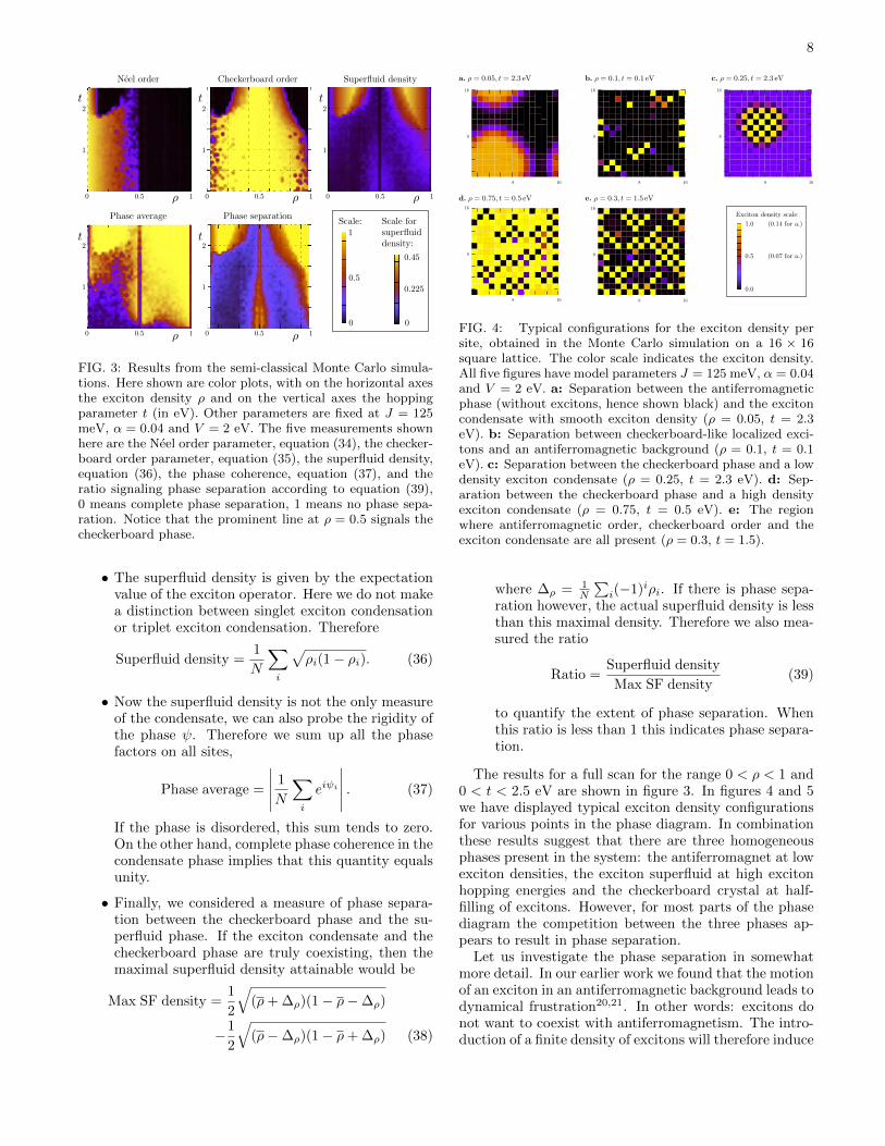
8

FIG. 3: Results from the semi-classical Monte Carlo simula-tions. Here shown are color plots, with on the horizontal axesthe exciton density ρ and on the vertical axes the hoppingparameter t (in eV). Other parameters are fixed at J = 125meV, α = 0.04 and V = 2 eV. The five measurements shownhere are the Neel order parameter, equation (34), the checker-board order parameter, equation (35), the superfluid density,equation (36), the phase coherence, equation (37), and theratio signaling phase separation according to equation (39),0 means complete phase separation, 1 means no phase sepa-ration. Notice that the prominent line at ρ = 0.5 signals thecheckerboard phase.

• The superfluid density is given by the expectationvalue of the exciton operator. Here we do not makea distinction between singlet exciton condensationor triplet exciton condensation. Therefore

Superfluid density =1

N

∑i

√ρi(1− ρi). (36)

• Now the superfluid density is not the only measureof the condensate, we can also probe the rigidity ofthe phase ψ. Therefore we sum up all the phasefactors on all sites,

Phase average =

∣∣∣∣∣ 1

N

∑i

eiψi

∣∣∣∣∣ . (37)

If the phase is disordered, this sum tends to zero.On the other hand, complete phase coherence in thecondensate phase implies that this quantity equalsunity.

• Finally, we considered a measure of phase separa-tion between the checkerboard phase and the su-perfluid phase. If the exciton condensate and thecheckerboard phase are truly coexisting, then themaximal superfluid density attainable would be

Max SF density =1

2

√(ρ+ ∆ρ)(1− ρ−∆ρ)

−1

2

√(ρ−∆ρ)(1− ρ+ ∆ρ) (38)

FIG. 4: Typical configurations for the exciton density persite, obtained in the Monte Carlo simulation on a 16 × 16square lattice. The color scale indicates the exciton density.All five figures have model parameters J = 125 meV, α = 0.04and V = 2 eV. a: Separation between the antiferromagneticphase (without excitons, hence shown black) and the excitoncondensate with smooth exciton density (ρ = 0.05, t = 2.3eV). b: Separation between checkerboard-like localized exci-tons and an antiferromagnetic background (ρ = 0.1, t = 0.1eV). c: Separation between the checkerboard phase and a lowdensity exciton condensate (ρ = 0.25, t = 2.3 eV). d: Sep-aration between the checkerboard phase and a high densityexciton condensate (ρ = 0.75, t = 0.5 eV). e: The regionwhere antiferromagnetic order, checkerboard order and theexciton condensate are all present (ρ = 0.3, t = 1.5).

where ∆ρ = 1N

∑i(−1)iρi. If there is phase sepa-

ration however, the actual superfluid density is lessthan this maximal density. Therefore we also mea-sured the ratio

Ratio =Superfluid density

Max SF density(39)

to quantify the extent of phase separation. Whenthis ratio is less than 1 this indicates phase separa-tion.

The results for a full scan for the range 0 < ρ < 1 and0 < t < 2.5 eV are shown in figure 3. In figures 4 and 5we have displayed typical exciton density configurationsfor various points in the phase diagram. In combinationthese results suggest that there are three homogeneousphases present in the system: the antiferromagnet at lowexciton densities, the exciton superfluid at high excitonhopping energies and the checkerboard crystal at half-filling of excitons. However, for most parts of the phasediagram the competition between the three phases ap-pears to result in phase separation.

Let us investigate the phase separation in somewhatmore detail. In our earlier work we found that the motionof an exciton in an antiferromagnetic background leads todynamical frustration20,21. In other words: excitons donot want to coexist with antiferromagnetism. The intro-duction of a finite density of excitons will therefore induce

9

FIG. 5: Different exciton configurations with their respectiveenergies on a 40× 40 lattice, to show whether there is macro-scopic phase separation. The model parameters are t = 0.5eV, J = 125 meV, α = 0.04, V = 2 eV and ρ = 0.06625.Yellow indicates the presence of excitons, and in the black re-gions there is antiferromagnetic order. a: The lowest energystate is the one with complete macroscopic phase separation.b: More complicated phase separation, such as the halterform depicted here, are higher in energy. c: Starting at hightemperatures with the configuration a, we slowly lowered thetemperature. The resulting configuration shown here is a lo-cal minimum. d: Using the same slow annealing as for cstarting from configuration b. The local energy minimum ob-tained this way is lower in energy than the configuration c.We conclude that even though macroscopic phase separationhas the lowest energy, there are many local energy minimawithout macroscopic phase separation.

phase separation. For large t, we find macroscopic phaseseparation between the antiferromagnet and the excitonsuperfluid, see figure 4a. At low exciton kinetic energythe excitons will crystallize in a checkerboard pattern ascan be seen in figure 4b.

Close to half-filling the role of the dipole repulsion Vbecomes increasingly relevant. The first order ‘spin flop’transition we discussed in section II B implies that therewill be phase separation between the superfluid and thecheckerboard order. Figures 4c and d show this phaseseparation. Finally there is a regime where the conden-sate, the checkerboard order and the Neel order are allpresent. However, given the dynamical frustration onthe one hand and the spin-flop transition on the otherhand, we again predict phase separation. A typical ex-citon configuration in this parameter regime is shown infigure 4e.

These simulated annealing results suggest that phaseseparation dominates the physics of this exciton system.To check whether the numerics are reliable we inspecteddirectly the energies of the various homogeneous mean

field solutions, using the Maxwell construction for phaseseparated states. The constructed phase separated con-figurations and their energies are shown in figure 5. Thelowest energy configuration (5a) has macroscopic phaseseparation between the checkerboard and the antiferro-magnetic phase. Intermediate states with one blob ofexcitons (5c) are slightly higher in energy than stateswith two blobs of excitons (5d). However, even thoughmacroscopic phase separation has the lowest energy, con-figurations with more blobs have more entropy. Conse-quently for any nonzero temperatures complete macro-scopic phase separation is not the most favorable solu-tion. This is indeed seen in the numerical simulations:annealing leads to high-entropy states such as figure 5drather than to the lowest energy configuration.

We thus conclude that the dominant phases are the an-tiferromagnet, the superfluid and the checkerboard. Thecompetition between these three phases leads to phaseseparation in most parts of the phase diagram. The unbi-ased Monte Carlo simulations show the direction in whichfurther analytical research should be directed: we will usemean field theory to characterize the three homogeneousphases.

C. Mean field theory and characterization of thephases

Given the fact that we are dealing with a hard-coreboson problem, we know that mean field theory is qual-itatively correct. A remaining issue is whether one cantune the exciton chemical potential rather than the ex-citon density in realistic experiments. Since we are pre-scient about the many first-order phase transitions in thissystem, we will perform the analysis with a fixed exci-ton density (the canonical ensemble). Using the Maxwellconstruction and the explicit µ vs. ρ relations, we cantransform back to the grand-canonical ensemble.

The numerical simulations suggest that the only solu-tions breaking translational symmetry invoke two sublat-tices,

ρi =

ρA i ∈ AρB i ∈ B (40)

and so forth for χ, θ, ψ and φ. This broken transla-tional symmetry allows for the antiferromagnetic andexciton checkerboard order. Evaluation of the energyE = 〈Ψ|H|Ψ〉 of the variational wavefunction, equation(31), directly suggests that we can set θ = ψ = φ = 0 onall sites.64 We are left with four parameters ρA, ρB , χAand χB , and as it turns out it will be more instructive to

10

0 0.5 10.750.25

1.0

2.0

3.0

4.0

PS: AF/CB

PS:AF/EC

PS: EC/CB

PS: EC/CB

EC EC

0.1 0.11.2

1.6

1.4

0.15

EC

PS: EC/CB

PS:AF/EC

PS: AF/CB

CO

FIG. 6: The canonical mean-field phase diagram for typi-cal values of J = 125 meV, α = 0.04 and V = 2 eV whilstvarying t and the exciton density ρ. In the absence of exci-ton, at ρ = 0, we have the pure antiferromagnetic Neel phase(AF). Exactly at half-filling of excitons (ρ = 1/2) and smallhoping energy t < 2V we find the checkerboard phase (CB)where one sublattice is filled with excitons and the other sub-lattice is filled with singlets. For large values of t we find thesinglet exciton condensate (EC), given by the wavefunction∏

i

(√ρE+

00,i +√

1− ρ)|0 0〉i. The coexistence of antiferro-

magnetism and superfluidity for small ρ and t is an artifactof the mean field theory. Conform the Monte Carlo results offigure 3, for most parts of the phase diagram phase separation(PS) is found.

rewrite these in terms of sum and difference variables,

ρ =1

2(ρA + ρB), (41)

∆ρ =1

2(ρA − ρB), (42)

χ = χA + χB , (43)

∆χ = χA − χB . (44)

The mean field energy per site is now given by

E/N =1

8Jz((1− ρ)2 −∆2

ρ

)(cos 2∆χ − cos 2χ)

−1

2J⊥ [(1− ρ)(cosχ cos ∆χ + 1)

+∆ρ sinχ sin ∆χ]

−1

4zt√

((1− ρ)2 −∆2ρ)(ρ

2 −∆2ρ) cos ∆χ

−µρ+1

2zV (ρ2 −∆2

ρ) (45)

which has to be minimized for a fixed average excitondensity ρ with the constraint |∆ρ| ≤ min(ρ, 1 − ρ). Theresulting mean field phase diagram for typical values ofJ, J⊥ and V , and for various t, ρ, is shown in figure 6.

1. Antiferromagnetic phase

As long as the exciton density is set to zero, the meanfield ground state is given by the ground state of thebilayer Heisenberg model,

ρ = 0, χ = 0 and cos ∆χ =J⊥Jz≡ α. (46)

The Neel order is given by

1

N

∑i

(−1)i〈Szi 〉 =√

1− α2 (47)

and the energy of the antiferromagnetic state is

E = −1

4Jz(1 + α)2. (48)

The introduction of excitons in an antiferromagneticbackground leads to dynamical frustration effects whichdisfavors the coexistence of excitons and antiferromag-netic order20,21. In fact, the numerical simulations al-ready ruled out coexistence of superfluidity and antifer-romagnetism.

2. Exciton condensate

For large exciton hopping energy t it becomes more fa-vorable to mix delocalized excitons into the ground state.Due to the bosonic nature of the problem this automati-cally leads to exciton condensation. The delocalized exci-tons completely destroy the antiferromagnetic order andthe exciton condensate is described by a superposition ofexcitons and a singlet background,

|Ψ〉 =∏i

(√ρ|Ei〉+

√1− ρ|0 0〉i

). (49)

Here we wish to emphasize the ubiquitous coupling tolight of the superfluid. The dipole matrix element allowsonly spin zero transitions, and since the exciton itself isS = 0 the dipole matrix element is directly related to thesuperfluid density,

〈∑σ

c†i1σci2σ〉 = 〈E|(c†1↑c2↑ + c†1↓c2↓

)|0 0〉

=1√2

√ρ(1− ρ)〈↑↓1 02|(

c†1↑c2↑ + c†1↓c2↓

)(| ↑1 ↓2〉 − | ↓1 ↑2〉)

=√

2ρ(1− ρ) (50)

The dipole matrix element thus acts as the order param-eter associated with the superfluid phase. In most bilayerexciton condensates, such as the one in the quantum Hallregime8, this order parameter is also nonzero in the nor-mal phase because of interlayer tunneling of electrons.One can therefore not speak strictly about spontaneousbreaking of U(1) symmetry in such systems; there is al-ready explicit symmetry breaking due to the interlayertunneling. In strongly correlated electron systems the fi-nite t⊥ is small compared to the chemical potential µ. Asdiscussed in the introduction, the Mott insulating bilay-ers now effectively allow for spontaneous U(1) symmetrybreaking, and the above dipole matrix element acts asa true order parameter. Note that the irrelevance of in-terlayer hopping t⊥ implies that this order parameter is,

11

unfortunately, not reflected in photon emission or inter-layer tunneling measurements.

The exciton condensate is a standard two-dimensionalBose condensate. The U(1) symmetry present in theXY -type exciton hopping terms is spontaneously brokenand we expect a linearly dispersing Goldstone mode inthe excitation spectrum, reflecting the rigidity of the con-densate. We will get back to the full excitation spectrumin section IV.

The energy of the singlet exciton condensate is

E = −J⊥ −(µ+ 1

4zt− J⊥)2

zt+ 2V z(51)

and the exciton density is given by

ρ = 2µ+ 1

4zt− J⊥zt+ 2V z

. (52)

3. Checkerboard phase

Whenever the exciton hopping is small, the introduc-tion of excitons into the system leads to the ‘spin flop’transition towards the checkerboard crystalline phase. Asshown in the context of the XXZ model, this phase im-plies that one sublattice is completely filled with exci-tons and the other sublattice is completely empty. Onthe empty sublattice, any nonzero J⊥ will guarantee thatthe singlet spin state has the lowest energy. Hence theaverage exciton density is here ρ = ∆ρ = 1/2 and theenergy of the checkerboard phase is given by

E = −1

2J⊥ −

1

2µ. (53)

It is interesting to note that the checkerboard phase isin fact similar to a Bose Mott insulator: with the new

doubled unit cell we have one exciton per unit cell. Thenearest neighbor dipole repulsion now acts as the ‘on-site’energy preventing extra excitons per unit cell.

4. Coexistence of antiferromagnetism and excitoncondensate

Within the analytical mean field theory set by equa-tion (45) there exists a small region where antiferromag-netism and the exciton condensate coexist. There the en-ergy of the homogenous coexistence phase is lower thanthe energy of macroscopic phase separation of the anti-ferromagnet and the condensate, as obtained using theMaxwell construction. However, within numerical sim-ulations we found no evidence of coexistence. Instead,we found microscopic phase separation, which hints ata possible complex inhomogeneous phase. We thereforeconclude that the homogeneous mean field theory dis-cussed here is insufficient to find the true ground state.

5. Exciton Mott insulator

Finally, when the exciton density is unity we have asystem composed of excitons only. In the parlance ofhard-core bosons this amounts to a exciton Mott insu-lator. This rather featureless phase is adiabatically con-nected to a standard electronic band insulator: the sys-tem is now composed of two layers where each layer hasan even number of electrons per unit cell. The energy ofthe exciton Mott insulator is, trivially

E = −µ+1

2V z. (54)

D. Phase separation

In this mean field theory most of the phase transitions are first order, with the exciton density varying discontinu-ously along the transition. The critical values of µ or t/J for the first order transitions are

µc,AF→CB =1

2Jz(1 + α2) (55)

µc,CB→EI = V z + J⊥ (56)

(t/J)c,AF→EC = 2(1 + α2)− 4µ

Jz+ 2

√(1− α2)

(4µ

Jz− (1 + α)2 − 2

V

J

)(57)

(t/J)c,CB→EC = 4

√( µJz− α

)(VJ

+ α− µ

Jz

)(58)

(t/J)c,CO→CB =2α2

2 µJz − 1

− 2α+

√(1− α2

2 µJz − 1

)(2

(V

J+ α− µ

Jz

)− α2

2 µJz − 1

). (59)

The transitions towards the coexistence region from the antiferromagnet or the condensate are second order. Addi-tionally, the transition from the condensate to the exciton Mott insulator is second order. The critical values of t/J

12

or µ at these second order transitions are

(t/J)c,AF→CO =2Jz(1 + α)− 4µ

J⊥(60)

(t/J)c,EC→CO = 1− 2µ

Jz+

√(1 + 8α) +

(2µ

Jz

)2

− 4

(3µ

Jz− 2V

J(1− α)

)(61)

µc,EC→EI = J⊥ +1

4zt+ V z. (62)

The subscripts indicate the phases: antiferromagneticphase (AF), coexistence phase (CO), exciton condensate(EC), exciton Mott insulator (EI), checkerboard phase(CB).

For any nonzero α the first order transitions fromthe antiferromagnetic or coexistence phase towards thecheckerboard phase are ‘standard’ in the sense that atthe critical value of µ there are only two mean field stateswith equal energy. This is also true for the transitionsfrom the antiferromagnet to the exciton condensate ex-cept at a single point. At the tricritical point

tc = 2J√

2V/J − 1 (63)

µc = J⊥ −1

4zt+

1

2Jz(1− α)

√2V/J + t/J (64)

separating the coexistence phase, the antiferromagneticphase and the exciton condensate, we can set the param-eters χ = 0, ∆ρ = 0 and ∆χ given by the value in thecoexistence phase. Now the energy becomes independentof the exciton density ρ. Similarly, at the critical valueof

µc = J⊥ +1

2V z ± 1

4

√(2V z)2 − (zt)2 (65)

describing the transition between the checkerboard phaseto the singlet exciton condensate, we can choose the meanfield parameters χ = 0, ∆χ = 0 and

∆ρ =1√2

√(1− 2ρ+ 2ρ2)− 2V |1− 2ρ|√

4V 2 − t2. (66)

With these parameters, the energy becomes independentof ρ.

This implies that the mean field theory predicts highlydegenerate states at the critical values of µ, similar to theone we found in the XXZ model. The phase separationthat thus occurs can be between an infinite set of pos-sible ground states that have all a different exciton den-sity. Coincidentally, the numerical simulations indicatethat around the two ‘degenerate’ critical points indeedall the three phases are present. While the macroscopicphase separated state might have the lowest energy, fig-ure 5 suggests that more complicated patterns of phaseseparation are likely to occur. The degeneracy of thecritical points on the level of mean fields theory might beresponsible for richer physics in these special regions ofthe phase diagram.

0 0.5 10.750.25

1.0

2.0

3.0

4.0

PS: AF/CB

PS:AF/EC

PS: EC/CB

PS: EC/CB

EC EC

PS: AF/EC/CB

FIG. 7: The canonical ground state phase diagram of the ex-citon t−J model, which is a combination of the semi-classicalMonte Carlo result and the mean field computations. In thebackground we have put the mean field phase diagram of fig-ure 6, whilst the lines show the phase diagram as obtainedfrom the Monte Carlo simulations. The dotted area representsphase separation between the condensate, antiferromagneticand checkerboard order. Furthermore: EC means excitoncondensate, CB means checkerboard phase, AF means anti-ferromagnetism and PS stands for phase separation.

E. Conclusion

Combining the simulated annealing results of figure 3with the analytical mean field results of figure 6 we ar-rive at the definitive mean field phase diagram of theexciton t − J model in figure 7. There are three mainphases: the antiferromagnet at zero exciton density, thecheckerboard crystal at exciton density ρ = 1/2 and thesuperfluid at high hopping energy t. For most parts ofthe phase diagram, phase separation between these threephases occurs in any possible combination. The com-petition between these three phases leads generally tomacroscopic phase separation.

Finally, within the limitations of the semi-classicalMonte Carlo approach we deduce an estimate of the tran-sition temperature towards the superfluid state. Givena typical point in the phase diagram where the excitoncondensate exists, at t = 2.5 eV and ρ = 0.18, we finda Kosterlitz-Thouless transition temperature of approxi-mately 700 Kelvin, see figure 3c. This number should be

13

0

0.2

0.4

0.6

0.8

1

0.01 0.1 1

T (eV)

N=10N=12N=16

Phase coherence, t=2.5 eV and ρ=0.18<φ

>

FIG. 8: Finite temperature graph of the phase coherencein the exciton condensate region of the phase diagram. Heret = 2.5 eV and ρ = 0.18 and the other parameters are thesame as in a. A clear transition is observed at around 0.06eV, which amounts to a transition temperature of about 700Kelvin.

taken not too seriously, as the exciton t−J model mightnot be applicable at such high temperatures given possi-ble exciton dissociation. Additionally, at high tempera-tures the electron-phonon coupling becomes increasinglyimportant, which we neglect in our exciton t− J model.Nonetheless, our estimate suggests that exciton superflu-idity may extend to quite high finite temperatures.

IV. COLLECTIVE MODES ANDSUSCEPTIBILITIES

Each phase of the excitons in the strongly correlatedbilayer has distinct collective modes, that are in princi-ple measurable by experiment. In order to obtain thedispersions of the collective modes we employ the tech-nique of the Heisenberg equations of motion, introducedin the context of the XXZ model in section II C and fur-ther formalized in Appendix B. In the case of the excitont− J model the set of equations is larger and analyticalsolutions can in general not be obtained. Whenever thisis the case we compute the dispersions numerically.

Quantities of direct experimental relevance are the dy-namical susceptibilities. We are for instance interestedin the absorptive part of the dynamical magnetic suscep-tibility, defined by

χ′′S(q, ω) =∑n

〈ψ0|S−(−q)|n〉〈n|S+(q)|ψ0〉δ(En − ω)

(67)Here |ψ0〉 is the ground state of the system and |n〉 are theexcited states with energy En. It appears unlikely thatbilayer exciton systems can be manufactured in bulk formwhich is required for neutron scattering, while there is areal potential to grow these using thin layer techniques.Therefore the detection of the dynamical spin suscepti-bility forms a realistic challenge for resonant inelastic X-ray scattering (RIXS)52 measurements with its claimedsensitivity for interface physics53.

Furthermore we are interested in the charge dynamicalsusceptibility

χ′′E(q, ω) =∑n

〈ψ0|E−00(−q)|n〉〈n|E+00(q)|ψ0〉δ(En − ω).

(68)which is directly related to the polarization propaga-tor. We use the operator E00(q) because this amountsto the interlayer dipole matrix element. Therefore, thischarge dynamical susceptibility expresses the excitonicexcitations. It can be observed by optical absorptionexperiments54 at q = 0. Finite wavelength measure-ments may be obtained using the aforementioned RIXS52

technique, or using electron energy loss spectroscopy(EELS)55,56. The method we use to compute the suscep-tibilities, based on the Heisenberg equations of motionmethod, is also described in Appendix B.

The three dominant phases we encountered in ourmean field analysis will have distinct magnetic and opti-cal responses. Let us briefly summarize our main findingswith respect to the collective excitations. The results forthe antiferromagnetic phase are shown in figures 9 to 11.This limit of vanishing exciton density has been stud-ied with in far greater rigor than our current Zubarevmethod is capable of20,21. We can therefore compare theresults of the Zubarev method with a full resummationof spin-exciton interactions using the self-consistent Bornapproximation (LSW-SCBA). It turns out that for smallexciton kinetic hopping t the non-interacting equations-of-motion method yields reliable results. For large t oneneeds the full SCBA code to correctly reproduce the dy-namical frustration effects of excitons in the antiferro-magnetic background.

The collective modes of the exciton condensate areshown in figures 12 and 13. Due to the absence of dynam-ical frustration and the presence of a spin-gap we expectthat these results survive in a fully interacting compu-tation. In fact, here the modes of the simple hard-coreboson system discussed in section II can be used as atemplate. Just as for the phase diagram, the qualitativefeatures of XXZ model are still of relevance for the morecomplicated t−J model. Nonetheless, in this condensatephase the interplay between excitonic and magnetic de-grees of freedom gives rise to a rather counterintuitiveeffect. We find that the exciton superfluid density canbe detected directly in a measurement of the magneticexcitations, as we already announced elsewhere37.

In contrast, in the checkerboard crystalline phase thespin and exciton degrees of freedom are once again de-coupled. In the remainder of this section we will elab-orate further on these results for each phase separately.Throughout the following discussion, the model parame-ters are J = 125 meV, α = 0.04, V = 2 eV and a varyingt and ρ. In order to visualize the susceptibilities we haveconvoluted χ′′ with a Lorentzian of width 0.04 eV. Thecolor scale of the susceptibility plots is in arbitrary units.

14

FIG. 9: The spin wave dispersions (a.) and the dynamicalmagnetic susceptibility (b.) in the antiferromagnetic phase.In this phase, the spin wave dispersions are not influencedby exciton dynamics. As is known from previous studies,there are two transversal spin waves and two longitudinal spinwaves21,29. The transversal spin waves are gapless around ei-ther Γ (solid red line) or the M point (dotted blue line). Thelongitudinal spin waves, which are associated with interlayerfluctuations (solid green line), are nearly flat and have a gapof order Jz. The dynamic magnetic susceptibility (b.) onlyshows one transversal spin wave. These results and all subse-quent figures are obtained using J = 125 meV and α = 0.04,as is expected for the undoped bilayer cuprate YBCO51.

A. Antiferromagnetic phase: a single exciton

In the limit of zero exciton density we recover the well-known bilayer Heisenberg physics29. As discussed in sec-tion III C, the spins tend to order antiferromagnetically.The excitations spectrum thus contains a Goldstone spinwave with linear dispersion around Γ and a similar modecentered around (π, π). In addition, the bilayer nature isreflected in the presence of two longitudinal spin waveswith a gap of order Jz and a narrow bandwidth of or-der J⊥. The excitation spectrum and the correspondingmagnetic dynamical susceptibility is shown in figure 9.Since the spin modes of the bilayer antiferromagnet areindependent of any exciton degrees of freedom, we willnot discuss these any further.

The dynamics of an isolated exciton in an antiferro-magnetic background has been studied extensively bymeans of a linear spin-wave self-consistent Born ap-proximation technique (LSW-SCBA)20,21. The non-interacting equations of motion method used in this pa-per, amounts to the complete neglect of exciton-spin in-teractions, while these are on the foreground of the (re-summed) LSW-SCBA computation. However, the mereexistence of LSW-SCBA results allows us to compareit with our current non-interacting calculations. Let ustherefore first go through the LSW-SCBA results. Therewe need to distinguish between two limits: the adia-batic limit with t J shown in figure 10, and the anti-adiabatic limit where t J shown in figure 11.

Consider a single exciton in an antiferromagnetic back-ground. Now if this exciton hops to a neighboring site,it will leave behind two spins that are ferromagneticallyaligned with their neighbors. This process is called dy-

FIG. 10: The exciton modes in the antiferromagnetic phasein the adiabatic regime t J . Here we have chosen t = 0.1eV, J = 125 meV and α = 0.04. Within the equations ofmotion picture there are four exciton modes (a.), which comein pairs of two with a small interlayer splitting. Due to theantiferromagnetic order the exciton bands are renormalizedwith respect to a free hard-core boson (b.). The susceptibilitycorresponding to the free exciton motion (c.) is verified bythe fully interacting LSW-SCBA results (d.). This is to beexpected: in the adiabatic regime spins react much faster thanthe exciton motion and the exciton still moves freely dressedby a spin polaron, reducing its bandwidth to order t2/J .

namical frustration and limits severely the motion of anexciton. In the adiabatic limit (t J) this causes theexciton bandwidth to be drastically reduced to an ordert2/J . In addition, the magnetic background acts as aconfining potential leading to small but detectable lad-der states at higher energies.

At the other hand, in the anti-adiabatic regime t Jexciton hopping will destroy the antiferromagnetic orderas it will be surrounded by a cloud of frustrated spins.The quasiparticle picture completely breaks down andthe spectral weight of the exciton is redistributed to awide incoherent spectral bump. The ladder spectrumarising from the effective confinement will still be visible,though smeared out.

The equations-of-motion method however ignores theeffects of spin-exciton interactions such as dynamicalfrustration. It treats the excitons as well-defined quasi-particles. As such we can already guess beforehand thatthe non-interacting results will be reliable in the adia-batic regime. Indeed, in the equations-of-motion methodwe find four exciton modes corresponding to either thesinglet E+

00 or m = 0 triplet exciton E+10 operator, just

as in the LSW-SCBA. When α→ 0 we can write out an

15

FIG. 11: The exciton modes in the antiferromagnetic phasein the antiadiabatic regime t J . Here we have chosen t = 2eV, J = 125 meV and α = 0.04.. Just like in figure 10 wefind four exciton bands (a.), renormalized with respect to thefree hard-core boson results (b.). However, upon inclusionof the interaction the free susceptibility (c.) gets extremelyrenormalized (d.). The large exciton kinetic energy togetherwith the relatively spin dynamics create an effective poten-tial for the exciton: the exciton becomes localized and theconfinement generates a ladder spectrum. Note that thus inthe antiadiabatic regime the free results (a., c.) cannot betrusted.

analytical expression for the non-interacting dispersions,

ωk,± = µ± 1

2

√(Jz)2 +

(1

2ztγk

)2

. (69)

where each branch is twofold degenerate. This degener-acy is lifted when α 6= 0, leading to a splitting of order αwhich is largest around Γ and M .

In the limit of t J the dispersions, equation (69),indeed result in an effective exciton bandwidth of ordert2/J , conform the fully interacting theory as can be seenin figure 10. The natural question then arises: how isit possible that in the present non-interacting theory theexciton bandwidth depends on the spin parameter J? Forsure, the effective exciton model introduced in sectionII has no such renormalization as is shown in figure 10.There the exciton bandwidth fully depends on zt.

However, it is important to realize that the exciton op-erators E+

s0,i do not commute with the antiferromagnetic

order parameter operator Szi . As a result the mean fieldenergy of exciting an exciton is shifted either up or down(depending on the sublattice) yielding a gap between thetwo exciton branches of O(Jz). Now for small t, propa-

gation of the exciton requires that one has to ’pay’ theenergy shift Jz to move through both sublattices. As aresult the effective hopping is reduced by a factor t/J .Therefore the exciton bandwidth renormalization, seenin the full LSW-SCBA, is already present at the meanfield level.

For large t/J however we will pay a price for theconvenience of the non-interacting equations of motionmethod. At the mean field level one still expects the dis-persions to be described by equation (69). However, uponinclusion of the interaction corrections this picture breaksdown completely. The bandwidth of the non-interactingexciton is of order zt, whereas in the interacting theoryan incoherent ladder spectrum of the same width arises.Thus for large t/J the non-interacting results cannot betrusted. However, this only applies to the antiferromag-netic phase due to the presence of dynamical frustration.In general, it appears that the non-interacting results arequalitatively correct in the absence of gapless modes thatneed to be excited in order for an exciton to move. Thiscondition is naturally met for the other two phases. Wetherefore expect that exciton-spin interactions only leadto qualitative changes in the antiferromagnetic phase.

By simple selection rules one can already conclude thatthe singlet exciton mode couples to light. As a conse-quence this is the mode that is visible in the charge dy-namical susceptibility, which is related to the polarizationpropagator. The exciton excitations are shown in figures10d (for t < J) and 11d (for t > J).

Finally, note that at the transition from the antiferro-magnetic phase to the checkerboard phase the gap in theexciton spectrum vanishes at (π, π).

B. Superfluid phase

The mode spectrum of superfluid phase, as shown infigures 12 and 13, is characterized by a linearly dispersingGoldstone mode associated with the broken U(1) symme-try. This superfluid phase mode has vanishing energy atthe Γ point, where we find the inescapable linear disper-sion relation

ωk =1

4√

2zt√

(1− ρ)ρ (1 + 2V/t) |k|+ . . . (70)

The speed of the superfluid phase mode is the same asfor the XXZ model in equation (28) up to a rescalingof the t and V parameters. Indeed, this speed is pro-portional to the superfluid density

√ρSF =

√ρ(1− ρ).

This mode can be seen in the charge susceptibility, fig-ures 12e and f. The Goldstone mode has a gap at (π, π)which decreases monotonically with increasing excitondensity. Precisely at the first order transition towardsthe checkerboard phase this gap closes. This mode soft-ening at (π, π) is reminiscent of the roton in superfluidHelium: the wavelength of the roton is the same as thelattice constant of solid Helium.

16

FIG. 12: Dispersions and susceptibilities of the Goldstonemode associated with the exciton condensate. We have set t =V = 2 eV, J = 125 meV and α = 0.04, and the exciton densityis either ρ = 0.15 (left column) or ρ = 0.27 (right column).a, b. In the simple hard-core boson model the condensatephase clearly show the superfluid phase mode, linear at smallmomenta. c,d. In the full t−J model the Goldstone mode hasa similar dispersion as in the XXZ model. The speed of themode scales with the superfluid density. At higher densitiesthe mode softens around (π, π), and when this gap closes afirst order transition to the checkerboard phase sets in. e,f.The absorptive part of the charge susceptibility, which can bemeasured with for example EELS or RIXS.

Next to the Goldstone mode there are two triplet exci-tations, shown in figure 13, each one three-fold degener-ate. The degeneracy obviously arises from the standardtriplet degeneracy m = −1, 0,+1. The two brancheshowever distinguish between exciton-dominated modesand spin-dominated modes, let us discuss them sepa-rately.

The spin-dominated modes have a gap of order ∆S =Jz√α(1 + α− ρ), which is similar to the triplet gap in

FIG. 13: Dispersions and magnetic susceptibilities of theexciton condensate. We have set t = V = 2 eV, J = 125meV and α = 0.04, and the exciton density is either ρ = 0.15(left column) or ρ = 0.27 (right column). a,b. As the excitoncondensate is spin singlet, we assume that the excitation spec-trum is governed by propagating triplet modes. These modeshave a gap of order J⊥ and a bandwidth of order Jz. c,d. Incontrast to the simple Heisenberg results, the actual tripletmodes have enhanced kinetics37. The modes are split in aspin-dominated branch with small gap and large bandwidthproportional to the superfluid density (e,f.); and an exciton-dominated branch with a large gap and a small bandwidth(g,h.).

17

the bilayer Heisenberg model for large α. However, thebandwidth of these excitations scales with t rather thanwith J , as would be customary in a system without ex-citon condensation (see figures 13a and b). We discussedthis in great detail in recent work37, so let us briefly re-view these results. In the absence of a excitons the mo-tion of triplets is governed by the Heisenberg superex-change yielding a bandwidth of order J . Now introduceFock operators e† = |E〉〈0| and t† = |1m〉〈0|, so that theexciton-triplet exchange equation (2) reads

− t∑〈ij〉

e†jeit†i tj . (71)

This is an interaction term, thus seemingly irrelevant tothe bandwidth of the triplet. However, when the excitoncondensation sets in the operator e† obtains an expecta-tion value, in fact 〈e†〉 =

√ρSF where ρSF is the conden-

sate density. Therefore the higher order exchange termyields a quadratic triplet hopping term

− tρSF∑〈ij〉

t†i tj (72)

and the bandwidth of the triplet excitations becomesof order ztρSF. Now remember that the exciton hop-ping energy t resulted, in second order perturbation the-ory, from the ratio t2e/V

′ where te is the electron hop-ping energy and V ′ is the nearest neighbor Coulombrepulsion20,21. The Heisenberg coupling however wasgiven by J = 2t2/U where U is the onsite Coulomb repul-sion. Since for obvious reasons U > V ′, we find that thetriplet bandwidth is enhanced whenever exciton conden-sation sets is. This enhancement is clearly visible in thespin susceptibility χ′′T , which allows for an experimentalprobe of the exciton superfluid density.

The other branch of triplet excitations is dominated bytriplet excitons, and is therefore barely visible in the spinsusceptibility and not visible in the exciton susceptibility(which only shows singlet excitons). That it is indeeddominated by triplet excitons can be inferred from com-puting the matrix elements of the operator E1m, whichare shown in figures 13g and h. Furthermore, the gap∆E = (V z+tz)ρ−µ is a function of exciton model param-eters only. The bandwidth of this mode is of order O(zt),relatively independent of the exciton density. As a re-sult, for large superfluid densities the exciton-dominatedmodes cross the spin-dominated triplet modes. One candirectly see this in the excitation spectrum for ρ = 0.27as shown in figure 13d.

We can compare the triplet spectrum to the mode spec-trum of the singlet phase of the bilayer Heisenberg model.When J⊥ J the ground state consists of only rungsinglets. The excitation towards a triplet state, shown infigures 13a and b, has a gap Jz

√α(α− 1) and a band-

width of order Jz, which is considerably smaller thanthe O(zt) bandwidth in the condensate. However, be-cause the topology of the triplet mode is the same weexpect that the effect of the spin-exciton interactions is

FIG. 14: The excitation spectrum of the checkerboard phase.a. In the simple hard-core boson model there are two excitonmodes associated with the ’doublon’ and the ’holon’ excita-tion. b. The spin modes are decoupled from the excitonmodes in the full t − J model. There is only one possiblespin excitation: changing the singlet groundstate into a non-propagating triplet. c. The exciton modes, on the other hand,can still propagate. The excitation of removing an exciton canpropagate through the checkerboard. d. The propagatingmode that changes an exciton into a singlet is detectable byoptical means and thus shows up in the charge susceptibility.

the same in the bilayer Heisenberg model as for the su-perfluid. Since earlier LSW-SCBA showed no changesin the spectrum due to interactions, we infer that thenon-interacting results for the superfluid are reliable.

To conclude our discussion of the excitations of thesuperfluid phase let us consider the influence of the in-terlayer tunneling. In the context of the XXZ modelwe noticed that interlayer tunneling has no qualitativeinfluence on the phase diagram itself. However, the pres-ence of a weak interlayer tunneling may act as potentialpinningthe phase57 opening a gap in the superfluid phasemode spectrum of order O(

√t⊥(V + t)). Persistent cur-

rents can still exist, but one needs to overcome this gapin order to get the exciton supercurrent flowing.

C. Checkerboard phase

The third homogeneous phase of the exciton t − Jmodel is the checkerboard phase. In this phase the unitcell is effectively doubled with one exciton per unit cell.This state is analogous to a Bose Mott insulator. Thetrivial excitations are then the doublon and the holon:create two bosons per unit cell which costs an energy

18

V z − µ or to remove the boson. The latter will generatea propagating exciton mode, with dispersion

ωk,pm =1

2

±V z +

√(V z)2 ±

(1

2ztγk

)2∓ µ± J⊥.

(73)There are two such propagating modes: one associatedwith the singlet exciton and one with the triplet exci-ton. Precisely at the transition towards the superfluidphase, one of these exciton waves becomes gapless. Notethat the arguments that lead to the bandwidth renormal-ization in the antiferromagnetic phase also apply here,leading to an exciton bandwidth of order t2/V . The dis-persions and the corresponding charge dynamical suscep-tibility can be seen in figure 14.

In the spin sector one can excite a localized spin tripleton the empty sublattice. The triplet gap is set by theinterlayer energy J⊥, and the dispersion is flat becausethis triplet cannot propagate, as can be seen in figure14b.

V. CONCLUSIONS AND DISCUSSION

We have studied the possibility of exciton condensationin strongly correlated electron bilayers. Starting from thedescription of the Mott state, with localized electrons,an exciton is defined as an interlayer bound state of adouble occupied and vacant site. In the strong couplinglimit, as of relevance to laboratory systems based on Mottinsulators, the physics of such a system is described bythe exciton t− J model, equation (6).

We constructed the ground state phase diagram (figure7), based on both numerical simulations and analyticalmean field theory. Three distinct phases are dominant:the antiferromagnetic phase, the checkerboard phase andthe exciton condensate. For most parts of the phase di-agram however, macroscopic phase separation will occurbetween these three phases.

Measurements of the spin and charge susceptibilitiesmay discern in which one of the three main phases a spe-cific system is in. The antiferromagnetic phase is char-acterized by a spin wave centered at (π, π), whilst in theexciton condensate the triplet bandwidth acts as a probefor the superfluid density (see figure 13 and Ref.37). Inthe checkerboard phase the spin degrees of freedom arereflected only in a localized triplet excitation at low en-ergy.

The charge dynamic susceptibility shows distinct qual-itative behavior depending on the phase. In the antiferro-magnet the spin-exciton interactions play an importantrole20,21. The superfluid phase is characterized by thevisibility of the condensate Goldstone mode, whereas thecheckerboard phase has propagating exciton waves withbandwidth O(t2/V ). Note however that since we expectphase separation to occur for most model parameters, re-alistic samples will likely display features from all phases

in its susceptibilities.

Our theoretical work presented here is largely basedon the assumption of strong coupling. In this limit, theexcitons behave as local hard-core bosons. If the excitonbinding energy is less dominant, the exciton will extendover more lattice sites and thus probably enable coexis-tence phases. On the other hand we expect that spin-exciton interactions destabilize the coexistence phases,since these interactions generally lead to frustration ef-fects. One could also wonder what happens if one in-cludes longer-ranged interactions for the excitons, withthe possibility of exciton stripes and incommensuratecharge ordered phases36. Next, we are dealing with firstorder phase transitions where small changes may have se-vere consequences. Combining all these effects may leadto significant changes in the phase diagram, most notablyin the regime where we predict phase separation.

Within the context of the strongly coupled exciton t−Jmodel, a weaker exciton binding energy can be incorpo-rated via interaction and hopping terms for the next near-est neighbors, next next nearest neighbors, etcetera. Thismight lead to complex ordered phases such as stripes58.Such phases are found in many strongly correlated elec-tron systems31,34, and studying these in the context ofthe simple bosonic exciton t − J model might shed newlight on the more troublesome fermionic t− J model.

In addition to stripy behavior other non-trivial ex-citon density profiles may occur when one considersa density imbalance between the electrons and holes.Semiconductor imbalanced systems are predicted to ex-hibit Fulde-Ferrell-Larkin-Ovchinnikov density modu-lated phases59,60. It is worthwhile to investigate whethersuch phase can exist in strongly correlated electron sys-tems.

Next to an improvement of the phase diagram, we canalso improve the susceptibilities by including the effect ofexciton-spin interactions. Similar to our earlier work20,21

on the interaction between excitons and spins in the limitof a single exciton, one could perform a diagrammatic ex-pansion of these interactions. We expect that, apart fromour earlier results in the antiferromagnetic phase, inclu-sion of spin-exciton interactions will not qualitatively al-ter the excitation spectra.

Experimentally, the close coupling of p- and n-dopedMott insulators is still relatively ill explored. However,important advances in complex oxide thin film growth,by techniques such as Molecular Beam Epitaxy (MBE)and Pulsed Laser Deposition (PLD) equipped with in situmonitoring tools such as Reflective High Energy Elec-tron Diffraction (RHEED) are making it possible now togrow multilayers of perovskite oxides - of which many areMott insulators - with unit cell precision. A complicatingfactor in fabricating multilayers of p- and n-doped per-ovskites, like the cuprate family from which also the high-Tc superconductors are derived, are the oftentimes con-flicting (de)-oxygenation requirements. Optimized depo-sition and post-anneal procedures have made it possiblehowever to make thin film contacts between n- and p-

19

doped superconducting cuprates61, which is now furtherbeing explored in our labs to create and study the paralleln-p combinations resembling the theoretical model.

An interesting additional system that can be includedin this endeavor is the 2-dimensional electron gas thatis formed at the interfaces between selected oxide band-insulators such as SrTiO3 and LaAlO3. In this respectit is noteworthy that in specific configurations, in par-ticular a 1 unit cell SrTiO3 layer on top of a 2 unit cellLaAlO3 layer grown on TiO2-terminated SrTiO−3, a sys-tem of a closely coupled 2-dimensional electron gas anda 2-dimensional hole gas has been realized17.

Finally we note that some cuprate high-Tc materialsappear to have an intrinsic stacking of electron-dopedand hole-doped CuO2 layers, such as Ba2Ca3Cu4O8F2

62,where one could look for excitonic effects.

Acknowledgments

This research was supported by the Dutch NWO foun-dation through a VICI grant. The authors thank SergeiMukhin and Kai Wu for helpful discussions.

Appendix A: SU(5) structure of the exciton t− Jmodel

In this appendix we will define the operators that com-pose the SU(5) dynamical Lie algebra, as described in thebeginning of section II A. From the bilayer Heisenberg wealready have the SO(4) spin subalgebra

Sz = |1+〉〈1 + | − |1−〉〈1− | (A1)

S+ =√

2 (|1+〉〈10|+ |10〉〈1− |) (A2)

Sz = −|0〉〈10| − |10〉〈0| (A3)

S+ =√

2 (|1+〉〈0| − |0〉〈1− |) (A4)

where we use the obvious short-handed notation for thesinglet and triplet kets and bras. The commutation rela-tion between these operators read[

Sa, Sb]

= iεabcSc (A5)[Sa, Sb

]=[Sa, Sb

]= iεabcSc (A6)[

Sa, Sb]

= iεabcSc. (A7)

There are 12 exciton operators in the XY -like part of theHamiltonian, which we denote by

E+sm = |E〉〈s m| (A8)

Ezsm =1

2(|E〉〈E| − |s m〉〈s m|) , (A9)

where s = 0, 1 and m = −s . . . + s, with commutationrelations [

E+sm, E

−sm

]= 2Ezsm (A10)[

Ezsm, E+sm

]= E+

sm. (A11)

If we consider commutators between E-operators withdifferent sm then we obtain operators that are fully spin-dependent. We find that the only nonzero commutatorsbetween Esm operators with ms 6= m′s′,[

E−sm, E+s′m′

]= |s m〉〈s′ m′| (A12)[

Ezsm, E+s′m′

]=

1

2E+s′m′ . (A13)

We need some more operators to close the spin SU(4)

subalgebra, therefore define T, T operators by (note that

(T z)† = −T z),

T+ =√

2 (|1+〉〈10| − |10〉〈1− |) (A14)

T z = |0〉〈10| − |10〉〈0| (A15)

T+ =√

2 (|1+〉〈0|+ |0〉〈1− |) . (A16)

To complete the spin SU(4) subalgebra we define

M+ = |1+〉〈1− | (A17)

and the corresponding M− = (M+)†. Finally, noticethat we have one operator too much in our listing, sincethere are only 24 operators in SU(5). Thus there ex-ists a linear dependency relation between some operators,which is

1

2Sz + Ez1+ − Ez1− = 0. (A18)

So when constructing the Heisenberg equations of mo-tion, we will exclude one of these three from our formal-ism. The most logical step is to throw out the combina-tion Ez1+ − Ez1− and leave the sum

Ez1m ≡ Ez1+ + Ez1−. (A19)

The 24 operators of our dynamical SU(5) algebra are the

three S-, three S-, two T -, three T -, two M - and elevenE-operators.

Appendix B: The Heisenberg equations of motionmethod

In this appendix we elaborate a bit further on theHeisenberg equations of motion method, as introducedin paragraph II C. The aim of this method is to findthe spectrum of excitations, building on the foundationsgiven by the mean field approximation. Given a full setof local operators A`i , we can construct the Heisenbergequations of motion

i∂tA`i = [A`i , H] (B1)

which is in general impossible to solve. We employ thenotation that i indicates the lattice site, and ` is the indexdenoting the type of operator. The right hand side ofthis equation contains products of operators at different

20

lattice sites. Such products can be decoupled within themean field approximation as49,50

A`iA`′

j → 〈A`i〉A`′

j +A`i〈A`′

j 〉 (B2)

where i and j are different lattice sites. Upon Fouriertransforming lattice position into momentum and timeinto energy, we thus obtain a set of linear equations forthe operators,

ωqA`(q, ω) = M ``′(q)A`′(q, ω). (B3)

The spectrum of excitations is simply found by solvingthis eigenvalue equation for the matrix M(q).

In order to find the matrix elements 〈n|A`(q)|0〉 thatenter in susceptibilities we need will introduce the fol-lowing scheme. Assume that the Hamiltonian is of theform

H =∑qn

ωqnα†qnαqn (B4)

where the sum over q runs over momenta, and n indi-cates the different excited states. Now α†qn is a creationoperator, and irrespective of whether we are dealing withfermions or bosons we have the following equations ofmotion

i∂tα†qn = −ωqnα†qn. (B5)

That is: every eigenvector of M ``′(q) corresponding to anegative eigenvalue can be identified as a creation oper-ator for one of the elementary excitations. However, theeigenvalue equation itself is not enough because it doesnot yield the proper normalization of α†. Since we havethe eigenvector solution

α†qn = Un`A`(q) (B6)

we can write out the (anti)commutation relation for α†qnin terms of the (anti)commutation relations for theA`(q).Upon requiring that on the mean field level the operatorsα†qn obey canonical commutation relations, that is forbosons

〈[αqn, α

†qn′

]〉 = δnn′ , (B7)

we obtain a proper normalization for the new creationoperators. We can invert the normalized matrix Un` to

express A`(q) in terms of the creation operators α†qn. Fi-

nally, using 〈n′|α†qn|0〉 = δnn′ we can compute the wanted

matrix element for A`(q).As an example of this technique we can compute the

matrix element |〈n|S+(q)|0〉|2 for the antiferromagneticHeisenberg model on a square lattice. The mean fieldground state is the Neel state, which leads to the follow-ing equations of motion,

i∂t

(S+qA

S+qB

)=

1

2Jz

(1 γq−γq −1

)(S+qA

S+qB

). (B8)

where the subscript A and B denote the two differentsublattices, and γq = 1

2 (cos qx + cos qy). We quite easilyinfer that the eigenvalues are

ωq = ±1

2Jz√

1− γ2q (B9)

and thus we have one eigenvector corresponding to a cre-ation operator, and one to an annihilation operator. Ifwe define (

α†

β

)= U

(S+qA

S+qB

)(B10)

then the commutation relations tell us that the eigenvec-tor matrix U must satisfy

1 = 〈[α, α†]〉 = −2u211〈SzA〉 − 2u212〈SzB〉 = −u211 + u212.(B11)

The initial S+q operator, which enters in the spin sus-

ceptibility, can be expressed in terms of the eigenvectormatrix as

S+q =1√2

(1 1) U−1(α†

β

). (B12)

Some straightforward algebra now yields

∣∣〈n|S+(q)|0〉∣∣2 =

1

2

√1− γq1 + γq

(B13)

which is the same susceptibility one can obtain by usingthe Holstein-Primakoff linear spin wave approximation.The approximation scheme we introduced here can there-fore be viewed as a generalization of the linear spin waveapproximation.

∗ Electronic address: rademaker@lorentz.leidenuniv.nl1 M. Imada M, A. Fujimori and Y. Tokura, Rev. Mod. Phys.

70, 1039 (1998).2 P. A. Lee, N. Nagaosa and X.-G. Wen, Rev. Mod. Phys.

78, 17 (2006).3 J. M. Blatt, K. W. Boer and W. Brandt, Phys. Rev. 126,

1691 (1962).4 L. Keldysh, A. Kozlov, Sov. Phys. JETP 27, 521 (1968).5 S. A. Moskalenko and D. W. Snoke, Bose-Einstein Conden-sation of Excitons and Biexcitons and Coherent NonlinearOptics with Excitons (Cambridge Univ. Press, Cambridge,2000).

21

6 S. I. Shevchenko, Fiz. Nizk. Temp. 2, 505 (1976); Sov. J.Low-Temp. Phys. 2, 251 (1976).

7 Yu. E. Lozovik and V. I. Yudson, Zh. Eksp. Teor. Fiz. 71,738 (1976); Sov. Phys. JETP 44, 389 (1976).

8 J. P. Eisenstein and A. H. MacDonald, Nature 432, 691(2004).

9 A. A. High, J. R. Leonard, M. Remeika, L. V. Butov, M.Hanson and A. C. Gossard, Nano Lett. 12, 2605 (2012).

10 B. Seradjeh, J. E. Moore and M. Franz, Phys. Rev. Lett.103, 066402 (2009).

11 Yu. E. Lozovik and A. A. Sokolik, JETP Lett. 87, 55(2008).

12 C.-H. Zhang and Y. N. Joglekar, Phys. Rev. B 77, 233405(2008).

13 R. Dillenschneider and J. H. Han, Phys. Rev. B 78, 045401(2008).

14 H. Min, R. Bistritzer, J.-J. Su and A. H. MacDonald, Phys.Rev. B 78, 121401(R) (2008).

15 M. Yu. Kharitonov and K. B. Efetov, Phys. Rev. B 78,241401(R) (2008).

16 T. C. Ribeiro, A. Seidel, J. H. Han and D.-H. Lee, Euro-phys. Lett. 76, 891 (2006).

17 R. Pentcheva et al., Phys. Rev. Lett. 104, 166804 (2010).18 A. J. Millis and D. G. Schlom, Phys. Rev. B 82, 073101

(2010).19 F. C. Zhang and K. K. Ng, Phys. Rev. B 58, 13520 (1998).20 L. Rademaker, K. Wu, H. Hilgenkamp and J. Zaanen, Eu-

rophys. Lett. 97, 27004 (2012).21 L. Rademaker, K. Wu and J. Zaanen, New J. Phys. 14,

083040 (2012).22 Z.-Y. Weng, Int. J. Mod. Phys. B 21, 773 (2007).23 S. Schmitt-Rink, C. M. Varma and A. E. Ruckenstein,

Phys. Rev. Lett. 60, 2793 (1988).24 C. L. Kane, P. A. Lee and N. Read, Phys. Rev. B 39, 6880

(1989).25 K. I. Kugel and D. I. Khomskii, Soviet Phys. Uspekhi 25,

231 (1982).26 C. N. A. van Duin and J. Zaanen, Phys. Rev. B 61, 3676

(2000).27 S.-C. Zhang, Science 275, 1089 (1997).28 D. Snoke, Nature 443, 403 (2006).29 A. V. Chubukov and D. K. Morr, Phys. Rev. B 52, 3521

(1995).30 J. Zaanen, Physica C 317-318, 217 (1999).31 J. Zaanen and O. Gunnarsson, Phys. Rev. B 40, 7391

(1989).32 V. J. Emery and S. A. Kivelson, Physica C 209, 597 (1993).33 U. Low, V. J. Emery, K. Fabricius and S. A. Kivelson,

Phys. Rev. Lett. 72, 1918 (1994).34 J. M. Tranquada, B. J. Sternlieb, J. D. Axe, Y. Nakamura,

S. Uchida, Nature 375, 561 (1995).35 N. G. Zhang and C. L. Henley, Phys. Rev. B 68, 014506

(2003).36 L. Rademaker, Y. Pramudya, J. Zaanen and V. Dobrosavl-

jevic, arXiv:1306.4765 (2013).37 L. Rademaker, J. Zaanen and H. Hilgenkamp, accepted by

Phys. Rev. B Rapid Communications (2013).38 E. Manousakis, Rev. Mod. Phys. 63, 1 (1991).39 C. N. A. van Duin, PhD-thesis, Leiden University ; C. N. A.

van Duin and J. Zaanen, Phys. Rev. Lett. 78, 3019 (1997).40 L. Neel, Ann. Phys. (Paris) 5, 232 (1936).41 M. E. Fisher and D. R. Nelson, Phys. Rev. Lett. 32, 1350

(1974).42 D. P. Landau and K. Binder, Phys. Rev. B 24, 1391 (1981).43 A. van Otterlo A et al, Phys. Rev. B 52, 16176 (1995).44 M. Kohno and M. Takahashi M, Phys. Rev. B 56, 3212

(1997).45 S. Yunoki, Phys. Rev. B 65, 092402 (2002).46 A. Kantian, A. J. Daley, P. Toermae and P. Zoller, New J.

Phys. 9, 407 (2007).47 J. M. Kosterlitz and D. J. Thouless, J. Phys. C 6, 1181

(1973).48 J. M. Yeomans, Statistical Mechanics of Phase Transitions

(Oxford Univ. Press, Oxford, 1992)49 D. N. Zubarev, Usp. Fiz. Nauk 71, 71 (1960); Sov. Phys.

Usp. 3, 320 (1960).50 A. M. Oles, L. F. Feiner and J. Zaanen, Phys. Rev. B 61,

6257 (2000).51 J. M. Tranquada et al, Phys. Rev. B 40, 4503 (1989).52 L. J. P. Ament et al, Rev. Mod. Phys. 83, 705 (2011).53 M. P. M. Dean et al, Nat. Mater. 11, 850 (2012).54 D. N. Basov and T. Timusk, Rev. Mod. Phys. 77, 721

(2005).55 S. E. Schnatterly, Solid State Phys. 24, 275 (1979).56 Y. Y. Wang et al, Phys. Rev. Lett. 77, 1809 (1996)57 L. Rademaker, J. Zaanen and H. Hilgenkamp, Phys. Rev.

B 83, 012504 (2011).58 M. M. Parish and F. M. Marchetti, Phys. Rev. Lett. 108,

145304 (2012).59 A. L. Subasi, P. Pieri, G. Senatore and B. Tanatar, Phys.

Rev. B 81, 075436 (2010).60 M. M. Parish, F. M. Marchetti and P. B. Littlewood, Eu-

rophys. Lett. 95, 27007 (2011).61 I. Takeuchi, S. N. Mao, X. X. Xi, K. Petersen, C. J. Lobb

and T. Venkatesan, Appl. Phys. Lett. 67, 2872 (1995).62 Y. Chen et al, Phys. Rev. Lett. 97, 236401 (2006).63 If we associate the presence of a particle with spin up,

and the absence with spin down, then the solid phaseis identified with an Ising antiferromagnet. However, oneshould not confuse this with the actual antiferromagnetismpresent in the spin sector of the full exciton t − J model.To avoid confusion, from now on we will use the term ’an-tiferromagnetism’ only when referring to the spin degreesof freedom in the full exciton t− J model.

64 By setting θ = φ = 0 we restrict the spin vectors to bepointing in the ±z direction only. Since we anticipate mag-netic ordering we have the freedom to choose the direc-tion of the ordering. Similar arguments hold for the choiceψ = 0; when breaking the U(1) symmetry associated withexciton condensation we are free to choose the phase di-rection.