package ‘qpgraph’ - bioconductor · package ‘qpgraph’ november 28, 2018 title estimation of...

Package ‘qpgraph’February 1, 2019

Title Estimation of genetic and molecular regulatory networks fromhigh-throughput genomics data

Version 2.16.0

DescriptionEstimate gene and eQTL networks from high-throughput expression and genotyping assays.

License GPL (>= 2)

Depends R (>= 3.4)

Imports methods, parallel, Matrix (>= 1.0), grid, annotate, graph (>=1.45.1), Biobase, S4Vectors, BiocParallel, AnnotationDbi,IRanges, GenomeInfoDb, GenomicRanges, GenomicFeatures, mvtnorm,qtl, Rgraphviz

Suggests RUnit, BiocGenerics, BiocStyle, genefilter, org.EcK12.eg.db,rlecuyer, snow, Category, GOstats

LazyData yes

URL https://github.com/rcastelo/qpgraph

BugReports https://github.com/rcastelo/rcastelo/issues

biocViews Microarray, GeneExpression, Transcription, Pathways,NetworkInference, GraphAndNetwork, GeneRegulation, Genetics,GeneticVariability, SNP, Software

git_url https://git.bioconductor.org/packages/qpgraph

git_branch RELEASE_3_8

git_last_commit c128a5f

git_last_commit_date 2018-10-30

Date/Publication 2019-01-31

Author Robert Castelo [aut, cre],Alberto Roverato [aut]

Maintainer Robert Castelo <[email protected]>

R topics documented:qpgraph-package . . . . . . . . . . . . . . . . . . . . . . . . . . . . . . . . . . . . . . 2EcoliOxygen . . . . . . . . . . . . . . . . . . . . . . . . . . . . . . . . . . . . . . . . 4eQTLcross-class . . . . . . . . . . . . . . . . . . . . . . . . . . . . . . . . . . . . . . 5

1

https://github.com/rcastelo/qpgraph

https://github.com/rcastelo/rcastelo/issues

2 qpgraph-package

eQTLnetwork-class . . . . . . . . . . . . . . . . . . . . . . . . . . . . . . . . . . . . . 5eQTLnetworkEstimate . . . . . . . . . . . . . . . . . . . . . . . . . . . . . . . . . . . 6eQTLnetworkEstimationParam-class . . . . . . . . . . . . . . . . . . . . . . . . . . . . 6graphParam-class . . . . . . . . . . . . . . . . . . . . . . . . . . . . . . . . . . . . . . 6HMgmm-class . . . . . . . . . . . . . . . . . . . . . . . . . . . . . . . . . . . . . . . . 7qpAllCItests . . . . . . . . . . . . . . . . . . . . . . . . . . . . . . . . . . . . . . . . . 8qpAnyGraph . . . . . . . . . . . . . . . . . . . . . . . . . . . . . . . . . . . . . . . . 10qpAvgNrr . . . . . . . . . . . . . . . . . . . . . . . . . . . . . . . . . . . . . . . . . . 12qpBoundary . . . . . . . . . . . . . . . . . . . . . . . . . . . . . . . . . . . . . . . . . 15qpCItest . . . . . . . . . . . . . . . . . . . . . . . . . . . . . . . . . . . . . . . . . . . 17qpClique . . . . . . . . . . . . . . . . . . . . . . . . . . . . . . . . . . . . . . . . . . . 19qpCliqueNumber . . . . . . . . . . . . . . . . . . . . . . . . . . . . . . . . . . . . . . 21qpCov . . . . . . . . . . . . . . . . . . . . . . . . . . . . . . . . . . . . . . . . . . . . 23qpEdgeNrr . . . . . . . . . . . . . . . . . . . . . . . . . . . . . . . . . . . . . . . . . . 24qpFunctionalCoherence . . . . . . . . . . . . . . . . . . . . . . . . . . . . . . . . . . . 27qpG2Sigma . . . . . . . . . . . . . . . . . . . . . . . . . . . . . . . . . . . . . . . . . 29qpGenNrr . . . . . . . . . . . . . . . . . . . . . . . . . . . . . . . . . . . . . . . . . . 31qpGetCliques . . . . . . . . . . . . . . . . . . . . . . . . . . . . . . . . . . . . . . . . 34qpGraph-class . . . . . . . . . . . . . . . . . . . . . . . . . . . . . . . . . . . . . . . . 36qpGraphDensity . . . . . . . . . . . . . . . . . . . . . . . . . . . . . . . . . . . . . . . 37qpHist . . . . . . . . . . . . . . . . . . . . . . . . . . . . . . . . . . . . . . . . . . . . 38qpHTF . . . . . . . . . . . . . . . . . . . . . . . . . . . . . . . . . . . . . . . . . . . . 40qpImportNrr . . . . . . . . . . . . . . . . . . . . . . . . . . . . . . . . . . . . . . . . . 41qpIPF . . . . . . . . . . . . . . . . . . . . . . . . . . . . . . . . . . . . . . . . . . . . 42qpK2ParCor . . . . . . . . . . . . . . . . . . . . . . . . . . . . . . . . . . . . . . . . . 44qpNrr . . . . . . . . . . . . . . . . . . . . . . . . . . . . . . . . . . . . . . . . . . . . 45qpPAC . . . . . . . . . . . . . . . . . . . . . . . . . . . . . . . . . . . . . . . . . . . . 48qpPathWeight . . . . . . . . . . . . . . . . . . . . . . . . . . . . . . . . . . . . . . . . 50qpPCC . . . . . . . . . . . . . . . . . . . . . . . . . . . . . . . . . . . . . . . . . . . . 52qpPlotMap . . . . . . . . . . . . . . . . . . . . . . . . . . . . . . . . . . . . . . . . . . 53qpPlotNetwork . . . . . . . . . . . . . . . . . . . . . . . . . . . . . . . . . . . . . . . 55qpPrecisionRecall . . . . . . . . . . . . . . . . . . . . . . . . . . . . . . . . . . . . . . 56qpPRscoreThreshold . . . . . . . . . . . . . . . . . . . . . . . . . . . . . . . . . . . . 58qpRndGraph . . . . . . . . . . . . . . . . . . . . . . . . . . . . . . . . . . . . . . . . . 59qpRndWishart . . . . . . . . . . . . . . . . . . . . . . . . . . . . . . . . . . . . . . . . 60qpTopPairs . . . . . . . . . . . . . . . . . . . . . . . . . . . . . . . . . . . . . . . . . 61qpUnifRndAssociation . . . . . . . . . . . . . . . . . . . . . . . . . . . . . . . . . . . 63qpUpdateCliquesRemoving . . . . . . . . . . . . . . . . . . . . . . . . . . . . . . . . . 64SsdMatrix-class . . . . . . . . . . . . . . . . . . . . . . . . . . . . . . . . . . . . . . . 65UGgmm-class . . . . . . . . . . . . . . . . . . . . . . . . . . . . . . . . . . . . . . . . 66

Index 68

qpgraph-package Estimation of genetic and molecular regulatory networks from high-throughput genomics data

Description

Estimate gene and eQTL networks from high-throughput expression and genotyping assays.

qpgraph-package 3

Functions

• qpNrr estimates non-rejection rates for every pair of variables.

• qpAvgNrr estimates average non-rejection rates for every pair of variables.

• qpGenNrr estimates generalized average non-rejection rates for every pair of variables.

• qpEdgeNrr estimate the non-rejection rate of one pair of variables.

• qpCItest performs a conditional independence test between two variables given a condition-ing set.

• qpHist plots the distribution of non-rejection rates.

• qpGraph obtains a qp-graph from a matrix of non-rejection rates.

• qpAnyGraph obtains an undirected graph from a matrix of pairwise measurements.

• qpGraphDensity calculates and plots the graph density as function of the non-rejection rate.

• qpCliqueNumber calculates the size of the largest maximal clique (the so-called clique numberor maximum clique size) in a given undirected graph.

• qpClique calculates and plots the size of the largest maximal clique (the so-called cliquenumber or maximum clique size) as function of the non-rejection rate.

• qpGetCliques finds the set of (maximal) cliques of a given undirected graph.

• qpRndWishart random generation for the Wishart distribution.

• qpCov calculates the sample covariance matrix, just as the function cov() but returning adspMatrix-class object which efficiently stores such a dense symmetric matrix.

• qpG2Sigma builds a random covariance matrix from an undrected graph. The inverse of theresulting matrix contains zeroes at the missing edges of the given undirected graph.

• qpUnifRndAssociation builds a matrix of uniformly random association values between -1 and +1 for all pairs of variables that follow from the number of variables given as inputargument.

• qpK2ParCor obtains the partial correlation coefficients from a given concentration matrix.

• qpIPF performs maximum likelihood estimation of a sample covariance matrix given the in-dependence constraints from an input list of (maximal) cliques.

• qpPAC estimates partial correlation coefficients and corresponding P-values for each edge in agiven undirected graph, from an input data set.

• qpPCC estimates pairwise Pearson correlation coefficients and their corresponding P-valuesbetween all pairs of variables from an input data set.

• qpRndGraph builds a random undirected graph with a bounded maximum connectivity degreeon every vertex.

• qpPrecisionRecall calculates the precision-recall curve for a given measure of associationbetween all pairs of variables in a matrix.

• qpPRscoreThreshold calculates the score threshold at a given precision or recall level froma given precision-recall curve.

• qpFunctionalCoherence estimates functional coherence of a given transcriptional regulatorynetwork using Gene Ontology annotations.

• qpTopPairs reports a top number of pairs of variables according to either an associationmeasure and/or occurring in a given reference graph.

4 EcoliOxygen

• qpPlotNetwork plots a network using the Rgraphviz library.

This package provides an implementation of the procedures described in (Castelo and Roverato,2006, 2009) and (Tur, Roverato and Castelo, 2014). An example of its use for reverse-engineeringof transcriptional regulatory networks from microarray data is available in the vignette qpTxRegNetand, the same directory, contains a pre-print of a book chapter describing the basic functionality ofthe package which serves the purpose of a basic users’s guide. This package is a contribution to theBioconductor (Gentleman et al., 2004) and gR (Lauritzen, 2002) projects.

Author(s)

R. Castelo and A. Roverato

References

Castelo, R. and Roverato, A. A robust procedure for Gaussian graphical model search from mi-croarray data with p larger than n. J. Mach. Learn. Res., 7:2621-2650, 2006.

Castelo, R. and Roverato, A. Reverse engineering molecular regulatory networks from microarraydata with qp-graphs. J. Comput. Biol. 16(2):213-227, 2009.

Gentleman, R.C., Carey, V.J., Bates, D.M., Bolstad, B., Dettling, M., Dudoit, S., Ellis, B., Gautier,L., Ge, Y., Gentry, J., Hornik, K. Hothorn, T., Huber, W., Iacus, S., Irizarry, R., Leisch, F., Li,C., Maechler, M. Rosinni, A.J., Sawitzki, G., Smith, C., Smyth, G., Tierney, L., Yang, T.Y.H. andZhang, J. Bioconductor: open software development for computational biology and bioinformatics.Genome Biol., 5:R80, 2004.

Lauritzen, S.L. gRaphical Models in R. R News, 3(2)39, 2002.

Tur, I., Roverato, A. and Castelo, R. Mapping eQTL networks with mixed graphical Markov mod-els. Genetics, 198:1377-1393, 2014.

EcoliOxygen Preprocessed microarray oxygen deprivation data and filtered Regu-lonDB data

Description

The data consist of two classes of objects, one containing normalized gene expression microar-ray data from Escherichia coli (E. coli) and the other containing a subset of filtered RegulonDBtranscription regulatory relationships on E. coli.

Usage

data(EcoliOxygen)

Format

gds680.eset ExpressionSet object containing n=43 experiments of various mutants under oxygen deprivation (Covert et al., 2004). The mutants were designed to monitor the response from E. coli during an oxygen shift in order to target the a priori most relevant part of the transcriptional network by using six strains with knockouts of five key transcriptional regulators in the oxygen response (arcA, appY, fnr, oxyR and soxS). The data was obtained by downloading the corresponding CEL files from the Gene Expression Omnibus (http://www.ncbi.nlm.nih.gov/geo) under accession GDS680 and then normalized using the rma() function from the affy package. Following the steps described in (Castelo and Roverato, 2009) probesets were mapped to Entrez Gene Identifiers and filtered such that the current ExpressionSet object contains a total of p=4205 genes. The slot featureNames has already the corresponding Entrez Gene IDs.subset.gds680.eset ExpressionSet object corresponding to a subset of gds680.eset defined by the transcription factor genes that were knocked-out in the experiments by Covert et al. (2004) and their putative targets according to the RegulonDB database version 6.1.filtered.regulon6.1 Data frame object containing a subset of the E. coli transcriptional network from RegulonDB 6.1 (Gama-Castro et al, 2008) obtained through the filtering steps described in (Castelo and Roverato, 2009). In this data frame each row corresponds to a transcriptional regulatory relationship and the first two columns contain Blattner IDs of the transcription factor and target genes, respectively, and the following two correspond to the same genes but specified by Entrez Gene IDs. The fifth column contains the direction of the regulation according to RegulonDB.subset.filtered.regulon6.1 Subset of filtered.regulon6.1 containing the transcriptional regulatory relationships in RegulonDB version 6.1 that involve the transcription factor genes which were knocked-out in the experiments by Covert et al. (2004).

http://www.ncbi.nlm.nih.gov/geo

eQTLcross-class 5

Source

Covert, M.W., Knight, E.M., Reed, J.L., Herrgard, M.J., and Palsson, B.O. Integrating high-throughputand computational data elucidates bacterial networks. Nature, 429(6987):92-96, 2004.

Gama-Castro, S., Jimenez-Jacinto, V., Peralta-Gil, M., Santos-Zavaleta, A., Penaloza-Spinola, M.I.,Contreras-Moreira, B., Segura-Salazar, J., Muniz-Rascado, L., Martinez-Flores, I., Salgado, H.,Bonavides-Martinez, C., Abreu-Goodger, C., Rodriguez-Penagos, C., Miranda-Rios, J., Morett,E., Merino, E., Huerta, A.M., Trevino-Quintanilla, L., and Collado-Vides, J. RegulonDB (version6.0): gene regulation model of Escherichia coli K-12 beyond transcription, active (experimental)annotated promoters and Textpresso navigation. Nucleic Acids Res., 36(Database issue):D120-124,2008.

References

Castelo, R. and Roverato, A. Reverse engineering molecular regulatory networks from microarraydata with qp-graphs. J. Comp. Biol., 16(2):213-227, 2009.

Examples

data(EcoliOxygen)ls()

eQTLcross-class eQTL experimental cross model class

Description

The expression quantitative trait loci (eQTL) experimental cross model class serves the purpose ofholding all necessary information to simulate genetical genomics data from an experimental cross.

Author(s)

R. Castelo

eQTLnetwork-class eQTL network model class

Description

The expression quantitative trait loci (eQTL) network class serves the purpose of holding the resultof estimating an eQTL network from genetical genomics data.

Author(s)

R. Castelo

See Also

eQTLnetworkEstimationParam-class eQTLcross-class

6 graphParam-class

eQTLnetworkEstimate Estimation of a eQTL network from genetical genomics data

Description

The methods eQTLnetworkEstimate() perform the estimation of eQTL networks from genet-ical genomics data using as input an eQTLnetworkEstimationParam object and, eventually, aeQTLnetwork-class object.

Author(s)

R. Castelo

See Also

eQTLnetworkEstimationParam eQTLnetwork-class

eQTLnetworkEstimationParam-class

eQTL network parameter model class

Description

The expression quantitative trait loci (eQTL) network parameter class serves the purpose of holdingthe parameter information to estimate an eQTL network from genetical genomics data with thefunction eQTLnetworkEstimate.

Author(s)

R. Castelo

See Also

eQTLnetworkEstimate eQTLnetwork-class

graphParam-class Graph parameter classes

Description

Graph parameter classes are defined to ease the simulation of different types of graphs by using asingle interface rgraphBAM().

Author(s)

R. Castelo

HMgmm-class 7

HMgmm-class Homogeneous mixed graphical Markov model

Description

The "HMgmm" class is the class of homogeneous mixed graphical Markov models defined within theqpgraph package to store simulate and manipulate this type of graphical Markov models (GMMs).

An homogeneous mixed GMM is a family of multivariate conditional Gaussian distributions onmixed discrete and continuous variables sharing a set of conditional independences encoded bymeans of a marked graph. Further details can be found in the book of Lauritzen (1996).

Objects from the Class

Objects can be created by calls of the form HMgmm(g, ...) corresponding to constructor methodsor rHMgmm(n, g, ...) corresponding to random simulation methods.

Slots

pI: Object of class "integer" storing the number of discrete random variables.

pY: Object of class "integer" storing the number of continuous random variables.

g: Object of class graphBAM-class storing the associated marked graph.

vtype: Object of class "factor" storing the type (discrete or continuous) of each random variable.

dLevels: Object of class "integer" storing the number of levels of each discrete random variable.

a: Object of class "numeric" storing the vector of additive linear effects on continuous variablesconnected to discrete ones.

rho: Object of class "numeric" storing the value of the marginal correlation between two contin-uous random variables.

sigma: Object of class dspMatrix-class storing the covariance matrix.

mean: Object of class "numeric" storing the mean vector.

eta2: Object of class "numeric" storing for each continuous variable connected to a discrete one,the fraction of variance of the continuous variable explained by the discrete one.

Methods

HMgmm(g) Constructor method where g can be either an adjacency matrix or a graphBAM-classobject.

rHMgmm(n, g) Constructor simulation method that allows one to simulate homogeneous mixedGMMs where n is the number of GMMs to simulate and g can be either a markedGraphParamobject, an adjacency matrix or a graphBAM-class object.

names(x) Accessor method to obtain the names of the elements in the object x that can be retrievedwith the $ accessor operator.

$ Accessor operator to retrieve elements of the object in an analogous way to a list.

dim(x) Dimension of the homogeneous mixed GMM corresponding to the number of discrete andcontinuous random variables.

dimnames(x) Names of the discrete and continuous random variables in the homogeneous mixedGMM.

8 qpAllCItests

show(object) Method to display some bits of information about the input homogeneous mixedGMM specified in object.

summary(object) Method to display a sumamry of the main features of the input homogeneousmixed GMM specified in object.

plot(x, ...) Method to plot the undirected graph associated to the the input homogeneous mixedGMM specified in x. It uses the plotting capabilities from the Rgraphviz library to whichfurther arguments specified in ... are further passed.

Author(s)

R. Castelo

References

Lauritzen, S.L. Graphical models. Oxford University Press, 1996.

See Also

UGgmm

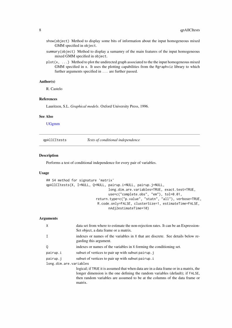
qpAllCItests Tests of conditional independence

Description

Performs a test of conditional independence for every pair of variables.

Usage

## S4 method for signature 'matrix'qpAllCItests(X, I=NULL, Q=NULL, pairup.i=NULL, pairup.j=NULL,

long.dim.are.variables=TRUE, exact.test=TRUE,use=c("complete.obs", "em"), tol=0.01,

return.type=c("p.value", "statn", "all"), verbose=TRUE,R.code.only=FALSE, clusterSize=1, estimateTime=FALSE,

nAdj2estimateTime=10)

Arguments

X data set from where to estimate the non-rejection rates. It can be an Expression-Set object, a data frame or a matrix.

I indexes or names of the variables in X that are discrete. See details below re-garding this argument.

Q indexes or names of the variables in X forming the conditioning set.

pairup.i subset of vertices to pair up with subset pairup.j

pairup.j subset of vertices to pair up with subset pairup.ilong.dim.are.variables

logical; if TRUE it is assumed that when data are in a data frame or in a matrix, thelonger dimension is the one defining the random variables (default); if FALSE,then random variables are assumed to be at the columns of the data frame ormatrix.

qpAllCItests 9

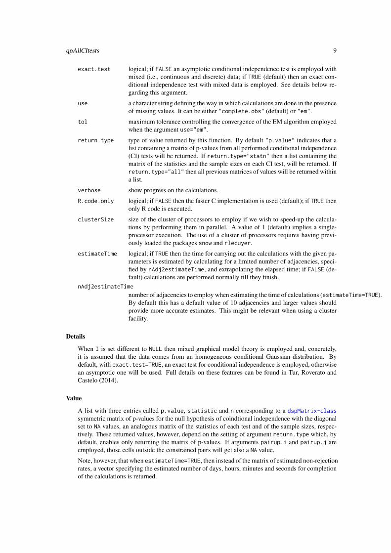
exact.test logical; if FALSE an asymptotic conditional independence test is employed withmixed (i.e., continuous and discrete) data; if TRUE (default) then an exact con-ditional independence test with mixed data is employed. See details below re-garding this argument.

use a character string defining the way in which calculations are done in the presenceof missing values. It can be either "complete.obs" (default) or "em".

tol maximum tolerance controlling the convergence of the EM algorithm employedwhen the argument use="em".

return.type type of value returned by this function. By default "p.value" indicates that alist containing a matrix of p-values from all performed conditional independence(CI) tests will be returned. If return.type="statn" then a list containing thematrix of the statistics and the sample sizes on each CI test, will be returned. Ifreturn.type="all" then all previous matrices of values will be returned withina list.

verbose show progress on the calculations.

R.code.only logical; if FALSE then the faster C implementation is used (default); if TRUE thenonly R code is executed.

clusterSize size of the cluster of processors to employ if we wish to speed-up the calcula-tions by performing them in parallel. A value of 1 (default) implies a single-processor execution. The use of a cluster of processors requires having previ-ously loaded the packages snow and rlecuyer.

estimateTime logical; if TRUE then the time for carrying out the calculations with the given pa-rameters is estimated by calculating for a limited number of adjacencies, speci-fied by nAdj2estimateTime, and extrapolating the elapsed time; if FALSE (de-fault) calculations are performed normally till they finish.

nAdj2estimateTime

number of adjacencies to employ when estimating the time of calculations (estimateTime=TRUE).By default this has a default value of 10 adjacencies and larger values shouldprovide more accurate estimates. This might be relevant when using a clusterfacility.

Details

When I is set different to NULL then mixed graphical model theory is employed and, concretely,it is assumed that the data comes from an homogeneous conditional Gaussian distribution. Bydefault, with exact.test=TRUE, an exact test for conditional independence is employed, otherwisean asymptotic one will be used. Full details on these features can be found in Tur, Roverato andCastelo (2014).

Value

A list with three entries called p.value, statistic and n corresponding to a dspMatrix-classsymmetric matrix of p-values for the null hypothesis of coindtional independence with the diagonalset to NA values, an analogous matrix of the statistics of each test and of the sample sizes, respec-tively. These returned values, however, depend on the setting of argument return.type which, bydefault, enables only returning the matrix of p-values. If arguments pairup.i and pairup.j areemployed, those cells outside the constrained pairs will get also a NA value.

Note, however, that when estimateTime=TRUE, then instead of the matrix of estimated non-rejectionrates, a vector specifying the estimated number of days, hours, minutes and seconds for completionof the calculations is returned.

10 qpAnyGraph

Author(s)

R. Castelo, A. Roverato and I. Tur

References

Castelo, R. and Roverato, A. A robust procedure for Gaussian graphical model search from mi-croarray data with p larger than n, J. Mach. Learn. Res., 7:2621-2650, 2006.


See Also

qpCItest

Examples

library(mvtnorm)

nVar <- 50 ## number of variablesmaxCon <- 3 ## maximum connectivity per variablenObs <- 30 ## number of observations to simulate

set.seed(123)

A <- qpRndGraph(p=nVar, d=maxCon)Sigma <- qpG2Sigma(A, rho=0.5)X <- rmvnorm(nObs, sigma=as.matrix(Sigma))

alltests <- qpAllCItests(X, verbose=FALSE)

## distribution of p-values for the present edgessummary(alltests$p.value[upper.tri(alltests$p.value) & A])

## distribution of p-values for the missing edgessummary(alltests$p.value[upper.tri(alltests$p.value) & !A])

qpAnyGraph A graph

Description

Obtains an undirected graph from a matrix of pairwise measurements

Usage

qpAnyGraph(measurementsMatrix, threshold=NA_real_, remove=c("below", "above"),topPairs=NA_integer_, decreasing=TRUE, pairup.i=NULL, pairup.j=NULL)

qpAnyGraph 11

Arguments

measurementsMatrix

matrix of pairwise measurements.

threshold threshold on the measurements below or above which pairs of variables are as-sumed to be disconnected in the resulting graph.

remove direction of the removal with the threshold. It should be either "below" (default)or "above".

topPairs number of edges from the top of the ranking, defined by the pairwise measure-ments in measurementsMatrix, to use to form the resulting graph. This param-eter is incompatible with a value different from NULL in threshold.

decreasing logical, only applies when topPairs is set; if TRUE then the ranking is made indecreasing order; if FALSE then is made in increasing order.


pairup.j subset of vertices to pair up with subset pairup.i

Details

This is a general purpose function for thresholding a matrix of pairwise measurements to selectpairs of variables corresponding to selected edges in an undirected graph.

Value

The resulting undirected graph as a graphBAM object. Note that when some gold-standard graphis available for comparison, a value for the parameter threshold can be found by calculating aprecision-recall curve with qpPrecisionRecall with respect to this gold-standard, and then usingqpPRscoreThreshold. Parameters threshold and topPairs are mutually exclusive, that is, whenwe specify with topPairs=n that we want a graph with n edges then threshold cannot be used.

Author(s)


References


See Also

qpNrr qpAvgNrr qpEdgeNrr qpGraph qpGraphDensity qpClique qpPrecisionRecall qpPRscoreThreshold

Examples

require(mvtnorm)require(graph)


set.seed(123)

12 qpAvgNrr


## estimate Pearson correlationspcc.estimates <- qpPCC(X)

## the higher the thresholdg <- qpAnyGraph(abs(pcc.estimates$R), threshold=0.9,

remove="below")

## the sparser the qp-graphnumEdges(g) / choose(numNodes(g), 2)

## the lower the thresholdg <- qpAnyGraph(abs(pcc.estimates$R), threshold=0.5,

remove="below")

# the denser the graphnumEdges(g) / choose(numNodes(g), 2)

qpAvgNrr Average non-rejection rate estimation

Description

Estimates average non-rejection rates for every pair of variables.

Usage

## S4 method for signature 'ExpressionSet'qpAvgNrr(X, qOrders=4, I=NULL, restrict.Q=NULL,

fix.Q=NULL, nTests=100, alpha=0.05,pairup.i=NULL, pairup.j=NULL, type=c("arith.mean"),

verbose=TRUE, identicalQs=TRUE,exact.test=TRUE, use=c("complete.obs", "em"),tol=0.01, R.code.only=FALSE, clusterSize=1,estimateTime=FALSE, nAdj2estimateTime=10)

## S4 method for signature 'data.frame'qpAvgNrr(X, qOrders=4, I=NULL, restrict.Q=NULL,

fix.Q=NULL, nTests=100, alpha=0.05, pairup.i=NULL,pairup.j=NULL, long.dim.are.variables=TRUE,type=c("arith.mean"), verbose=TRUE,identicalQs=TRUE, exact.test=TRUE,

use=c("complete.obs", "em"), tol=0.01, R.code.only=FALSE,clusterSize=1, estimateTime=FALSE, nAdj2estimateTime=10)

## S4 method for signature 'matrix'qpAvgNrr(X, qOrders=4, I=NULL, restrict.Q=NULL, fix.Q=NULL,

nTests=100, alpha=0.05, pairup.i=NULL,pairup.j=NULL, long.dim.are.variables=TRUE,type=c("arith.mean"), verbose=TRUE,identicalQs=TRUE, exact.test=TRUE,


qpAvgNrr 13

Arguments

X data set from where to estimate the average non-rejection rates. It can be anExpressionSet object, a data frame or a matrix.

qOrders either a number of partial-correlation orders or a vector of vector of particularorders to be employed in the calculation.

I indexes or names of the variables in X that are discrete. When X is an ExpressionSetthen I may contain only names of the phenotypic variables in X. See details be-low regarding this argument.

restrict.Q indexes or names of the variables in X that restrict the sample space of condi-tioning subsets Q.

fix.Q indexes or names of the variables in X that should be fixed within every condi-tioning conditioning subsets Q.

nTests number of tests to perform for each pair for variables.

alpha significance level of each test.



logical; if TRUE it is assumed that when the data is a data frame or a matrix,the longer dimension is the one defining the random variables; if FALSE, thenrandom variables are assumed to be at the columns of the data frame or matrix.

type type of average. By now only the arithmetic mean is available.


identicalQs use identical conditioning subsets for every pair of vertices (default), otherwisesample a new collection of nTests subsets for each pair of vertices.

exact.test logical; if FALSE an asymptotic conditional independence test is employed withmixed (i.e., continuous and discrete) data; if TRUE (default) then an exact condi-tional independence test with mixed data is employed.






nAdj2estimateTime


14 qpAvgNrr

Details

Note that when specifying a vector of particular orders q, these values should be in the range 1 tomin(p, n-3), where p is the number of variables and n the number of observations. The computa-tional cost increases linearly within each q value and quadratically in p. When setting identicalQsto FALSE the computational cost may increase between 2 times and one order of magnitude (depend-ing on p and q) while asymptotically the estimation of the non-rejection rate converges to the samevalue.

When I is set different to NULL then mixed graphical model theory is employed and, concretely,it is assumed that the data comes from an homogeneous conditional Gaussian distribution. In thissetting further restrictions to the maximum value of q apply, concretely, it cannot be smaller than pplus the number of levels of the discrete variables involved in the marginal distributions employedby the algorithm. By default, with exact.test=TRUE, an exact test for conditional independence isemployed, otherwise an asymptotic one will be used. Full details on these features can be found inTur, Roverato and Castelo (2014).

Value

A dspMatrix-class symmetric matrix of estimated average non-rejection rates with the diago-nal set to NA values. When using the arguments pairup.i and pairup.j, those cells outside theconstraint pairs will get also a NA value.

Note, however, that when estimateTime=TRUE, then instead of the matrix of estimated averagenon-rejection rates, a vector specifying the estimated number of days, hours, minutes and secondsfor completion of the calculations is returned.

Author(s)


References



See Also

qpNrr qpEdgeNrr qpHist qpGraphDensity qpClique

Examples

require(mvtnorm)


set.seed(123)


qpBoundary 15

avgnrr.estimates <- qpAvgNrr(X, verbose=FALSE)

## distribution of average non-rejection rates for the present edgessummary(avgnrr.estimates[upper.tri(avgnrr.estimates) & A])

## distribution of average non-rejection rates for the missing edgessummary(avgnrr.estimates[upper.tri(avgnrr.estimates) & !A])

## Not run:library(snow)library(rlecuyer)

## only for moderate and large numbers of variables the## use of a cluster of processors speeds up the calculations

nVar <- 500maxCon <- 3A <- qpRndGraph(p=nVar, d=maxCon)Sigma <- qpG2Sigma(A, rho=0.5)X <- rmvnorm(nObs, sigma=as.matrix(Sigma))

system.time(avgnrr.estimates <- qpAvgNrr(X, q=10, verbose=TRUE))system.time(avgnrr.estimates <- qpAvgNrr(X, q=10, verbose=TRUE, clusterSize=4))

## End(Not run)

qpBoundary Maximum boundary size of the resulting qp-graphs

Description

Calculates and plots the size of the largest vertex boundary as function of the non-rejection rate.

Usage

qpBoundary(nrrMatrix, n=NA, threshold.lim=c(0,1), breaks=5, vertexSubset=NULL,plot=TRUE, qpBoundaryOutput=NULL, density.digits=0, logscale.bdsize=FALSE,titlebd="Maximum boundary size as function of threshold", verbose=FALSE)

Arguments

nrrMatrix matrix of non-rejection rates.

n number of observations from where the non-rejection rates were estimated.

threshold.lim range of threshold values on the non-rejection rate.

breaks either a number of threshold bins or a vector of threshold breakpoints.

vertexSubset subset of vertices for which their maximum boundary size is calculated withrespect to all other vertices.

plot logical; if TRUE makes a plot of the result; if FALSE it does not.qpBoundaryOutput

output from a previous call to qpBoundary. This allows one to plot the resultchanging some of the plotting parameters without having to do the calculationagain.

16 qpBoundary

density.digits number of digits in the reported graph densities.logscale.bdsize

logical; if TRUE then the scale for the maximum boundary size is logarithmicwhich is useful when working with more than 1000 variables; FALSE otherwise(default).

titlebd main title to be shown in the plot.

verbose show progress on calculations.

Details

The maximum boundary is calculated as the largest degree among all vertices of a given qp-graph.

Value

A list with the maximum boundary size and graph density as function of threshold, the threshold onthe non-rejection rate that provides a maximum boundary size strictly smaller than the sample sizen and the resulting maximum boundary size.

Author(s)


References


See Also

qpHTF qpGraphDensity

Examples

require(mvtnorm)


set.seed(123)


## the higher the q the less complex the qp-graph

nrr.estimates <- qpNrr(X, q=1, verbose=FALSE)

qpBoundary(nrr.estimates, plot=FALSE)


qpBoundary(nrr.estimates, plot=FALSE)

qpCItest 17

qpCItest Conditional independence test

Description

Performs a conditional independence test between two variables given a conditioning set.

Usage

## S4 method for signature 'ExpressionSet'qpCItest(X, i=1, j=2, Q=c(), exact.test=TRUE, use=c("complete.obs", "em"),

tol=0.01, R.code.only=FALSE)## S4 method for signature 'cross'qpCItest(X, i=1, j=2, Q=c(), exact.test=TRUE, use=c("complete.obs", "em"),

tol=0.01, R.code.only=FALSE)## S4 method for signature 'data.frame'qpCItest(X, i=1, j=2, Q=c(), I=NULL, long.dim.are.variables=TRUE,

exact.test=TRUE, use=c("complete.obs", "em"), tol=0.01, R.code.only=FALSE)## S4 method for signature 'matrix'qpCItest(X, i=1, j=2, Q=c(), I=NULL, long.dim.are.variables=TRUE,

exact.test=TRUE, use=c("complete.obs", "em"), tol=0.01, R.code.only=FALSE)## S4 method for signature 'SsdMatrix'qpCItest(X, i=1, j=2, Q=c(), R.code.only=FALSE)

Arguments

X data set where the test should be performed. It can be either an ExpressionSetobject, a qtl::cross object, a data frame, a matrix or an SsdMatrix-classobject. In the latter case, the input matrix should correspond to a sample covari-ance matrix of data on which we want to test for conditional independence. Thefunction qpCov() can be used to estimate such matrices.

i index or name of one of the two variables in X to test.

j index or name of the other variable in X to test.

Q indexes or names of the variables in X forming the conditioning set.


long.dim.are.variables

logical; if TRUE it is assumed that when data are in a data frame or in a ma-trix, the longer dimension is the one defining the random variables (default);if FALSE, then random variables are assumed to be at the columns of the dataframe or matrix.

exact.test logical; if FALSE an asymptotic likelihood ratio test of conditional independencetest is employed with mixed (i.e., continuous and discrete) data; if TRUE (default)then an exact likelihood ratio test of conditional independence with mixed datais employed. See details below regarding this argument.



18 qpCItest

R.code.only logical; if FALSE then the faster C implementation is used (default); if TRUEthen only R code is executed.

Details

When variables in i, j and Q are continuous and I=NULL, this function performs a conditionalindependence test using a t-test for zero partial regression coefficient (Lauritzen, 1996, pg. 150).Note that the size of possible Q sets should be in the range 1 to min(p,n-3), where p is the numberof variables and n the number of observations. The computational cost increases linearly with thenumber of variables in Q.

When variables in i, j and Q are continuous and discrete (mixed data), indicated with the I ar-gument when X is a matrix, then mixed graphical model theory (Lauritzen and Wermuth, 1989) isemployed and, concretely, it is assumed that data come from an homogeneous conditional Gaussiandistribution. By default, with exact.test=TRUE, an exact likelihood ratio test for conditional inde-pendence is performed (Lauritzen, 1996, pg. 192-194; Tur, Roverato and Castelo, 2014), otherwisean asymptotic one is used.

In this setting further restrictions to the maximum value of q apply, concretely, it cannot be smallerthan p plus the number of levels of the discrete variables involved in the marginal distributionsemployed by the algorithm.

Value

A list with class "htest" containing the following components:

statistic in case of pure continuous data and I=NULL, the t-statistic for zero partial re-gression coefficient; when I!=NULL, the value Lambda of the likelihood ratio ifexact.test=TRUE and -n log Lambda otherwise.

parameter in case of pure continuous data and I=NULL, the degrees of freedom for the t-statistic (n-q-2); when I!=NULL, the degrees of freedom for -n log Lambdaof a chi-square distribution under the null hypothesis if exact.test=FALSE andthe (a, b) parameters of a beta distribution under the null if exact.test=TRUE.

p.value the p-value for the test.

estimate in case of pure continuous data (I=NULL), the estimated partial regression coeffi-cient. In case of mixed continuous and discrete data with I!=NULL, the estimatedpartial eta-squared: the fraction of variance from i or j explained by the othertested variable after excluding the variance explained by the variables in Q. Ifone of the tested variables i or j is discrete, then the partial eta-squared is cal-culated on the tested continuous variable. If both, i and j are continuous, thenthe partial eta-squared is calculated on variable i.

alternative a character string describing the alternative hypothesis.

method a character string indicating what type of conditional independence test wasperformed.

data.name a character string giving the name(s) of the random variables involved in theconditional independence test.

Author(s)


qpClique 19

References



Lauritzen, S.L and Wermuth, N. Graphical Models for associations between variables, some ofwhich are qualitative and some quantitative. Ann. Stat., 17(1):31-57, 1989.


See Also

qpCov qpNrr qpEdgeNrr

Examples

require(mvtnorm)

nObs <- 100 ## number of observations to simulate

## the following adjacency matrix describes an undirected graph## where vertex 3 is conditionally independent of 4 given 1 AND 2A <- matrix(c(FALSE, TRUE, TRUE, TRUE,

TRUE, FALSE, TRUE, TRUE,TRUE, TRUE, FALSE, FALSE,TRUE, TRUE, FALSE, FALSE), nrow=4, ncol=4, byrow=TRUE)

Sigma <- qpG2Sigma(A, rho=0.5)

X <- rmvnorm(nObs, sigma=as.matrix(Sigma))

qpCItest(X, i=3, j=4, Q=1, long.dim.are.variables=FALSE)

qpCItest(X, i=3, j=4, Q=c(1,2), long.dim.are.variables=FALSE)

qpClique Complexity of the resulting qp-graphs

Description

Calculates and plots the size of the largest maximal clique (the so-called clique number or maximumclique size) as function of the non-rejection rate.

Usage

qpClique(nrrMatrix, n=NA, threshold.lim=c(0,1), breaks=5, plot=TRUE,exact.calculation=TRUE, approx.iter=100,qpCliqueOutput=NULL, density.digits=0,logscale.clqsize=FALSE,titleclq="maximum clique size as function of threshold",verbose=FALSE)

20 qpClique

Arguments


n number of observations from where the non-rejection rates were estimated.



plot logical; if TRUE makes a plot of the result; if FALSE it does not.exact.calculation

logical; if TRUE then the exact clique number is calculated; if FALSE then alower bound is given instead.

approx.iter number of iterations to be employed in the calculation of the lower bound (i.e.,only applies when exact.calculation=FALSE).

qpCliqueOutput output from a previous call to qpClique. This allows one to plot the resultchanging some of the plotting parameters without having to do the calculationagain.

density.digits number of digits in the reported graph densities.logscale.clqsize

logical; if TRUE then the scale for the maximum clique size is logarithmic whichis useful when working with more than 1000 variables; FALSE otherwise (de-fault).

titleclq main title to be shown in the plot.


Details

The estimate of the complexity of the resulting qp-graphs is calculated as the area enclosed underthe curve of maximum clique sizes.

The maximum clique size, or clique number, is obtained by calling the function qpCliqueNumberThe calculation of the clique number of an undirected graph is an NP-complete problem whichmeans that its computational cost is bounded by an exponential running time (Pardalos and Xue,1994). Therefore, giving breakpoints between 0.95 and 1.0 may result into very dense graphs whichcan lead to extremely long execution times. If it is necessary to look at that range of breakpoints itis recommended either to use the lower bound on the clique number (exact.calculation=FALSE)or to look at qpGraphDensity.

Value

A list with the maximum clique size and graph density as function of threshold, an estimate ofthe complexity of the resulting qp-graphs across the thresholds, the threshold on the non-rejectionrate that provides a maximum clique size strictly smaller than the sample size n and the resultingmaximum clique size.

Author(s)


References


Pardalos, P.M. and Xue, J. The maximum clique problem. J. Global Optim., 4:301-328, 1994.

qpCliqueNumber 21

See Also

qpCliqueNumber qpGraphDensity

Examples

require(mvtnorm)


set.seed(123)


## the higher the q the less complex the qp-graph


qpClique(nrr.estimates, plot=FALSE)$complexity


qpClique(nrr.estimates, plot=FALSE)$complexity

qpCliqueNumber Clique number

Description

Calculates the size of the largest maximal clique (the so-called clique number or maximum cliquesize) in a given undirected graph.

Usage

qpCliqueNumber(g, exact.calculation=TRUE, return.vertices=FALSE,approx.iter=100, verbose=TRUE, R.code.only)

Arguments

g either a graphNEL object or an adjacency matrix of the given undirected graph.exact.calculation

logical; if TRUE then the exact clique number is calculated; if FALSE then alower bound is given instead.

return.vertices

logical; if TRUE a set of vertices forming a maximal clique of maximum size isreturned; if FALSE only the maximum clique size is returned.

approx.iter number of iterations to be employed in the calculation of the lower bound (i.e.,only applies when exact.calculation=FALSE.


22 qpCliqueNumber


Details

The calculation of the clique number of an undirected graph is one of the basic NP-complete prob-lems (Karp, 1972) which means that its computational cost is bounded by an exponential runningtime (Pardalos and Xue, 1994). The current implementation uses C code from the GNU GPL Cli-quer library by Niskanen and Ostergard (2003) based on the, probably the fastest to date, algorithmby Ostergard (2002).

The lower bound on the maximum clique size is calculated by ranking the vertices by their connec-tivity degree, put the first vertex in a set and go through the rest of the ranking adding those verticesto the set that form a clique with the vertices currently within the set. Once the entire ranking hasbeen examined a large clique should have been built and eventually one of the largests ones. Thisprocess is repeated a number of times (approx.iter) each of which the ranking is altered withincreasing levels of randomness acyclically (altering 1 to $p$ vertices and again). Larger values ofapprox.iter should provide tighter lower bounds although it has been proven that no polynomialtime algorithm can approximate the maximum clique size within a factor of nε (ε > 0), unlessP=NP (Feige et al, 1991; Pardalos and Xue, 1994).

Value

a lower bound of the size of the largest maximal clique in the given graph, also known as its cliquenumber.

Author(s)

R. Castelo

References


Feige, U., Goldwasser, S., Lov\’asz, L., Safra, S. and Szegedy, M. Approximating the maximumclique is almost NP-Complete. Proc. 32nd IEEE Symp. on Foundations of Computer Science, 2-12,1991.

Karp, R.M. Reducibility among combinatorial problems. Complexity of computer computations,43:85-103, 1972.

Niskanen, S. Ostergard, P. Cliquer User’s Guide, Version 1.0. Communications Laboratory, HelsinkiUniversity of Technology, Espoo, Finland, Tech. Rep. T48, 2003. (http://users.tkk.fi/~pat/cliquer.html)

Ostergard, P. A fast algorithm for the maximum clique problem. Discrete Appl. Math. 120:197-207,2002.

Pardalos, P.M. and Xue, J. The maximum clique problem. J. Global Optim., 4:301-328, 1994.

See Also

qpClique

http://users.tkk.fi/~pat/cliquer.html


qpCov 23

Examples

require(graph)

nVar <- 50

set.seed(123)

g1 <- randomEGraph(V=as.character(1:nVar), p=0.3)qpCliqueNumber(g1, verbose=FALSE)

g2 <- randomEGraph(V=as.character(1:nVar), p=0.7)qpCliqueNumber(g2, verbose=FALSE)

qpCov Calculation of the sample covariance matrix

Description

Calculates the sample covariance matrix, just as the function cov() but returning a dspMatrix-classobject which efficiently stores such a dense symmetric matrix.

Usage

qpCov(X, corrected=TRUE)

Arguments

X data set from where to calculate the sample covariance matrix. As the cov()function, it assumes the columns correspond to random variables and the rowsto multivariate observations.

corrected flag set to TRUE when calculating the sample covariance matrix (default; and setto FALSE when calculating the uncorrected sum of squares and deviations.

Details

This function makes the same calculation as the cov function but returns a sample covariance matrixstored in the space-efficient class dspMatrix-class and, moreover, allows one for calculating theuncorrected sum of squares and deviations which equals (n-1) * cov().

Value

A sample covariance matrix stored as a dspMatrix-class object. See the Matrix package for fulldetails on this object class.

Author(s)

R. Castelo

See Also

qpPCC

24 qpEdgeNrr

Examples

require(graph)require(mvtnorm)

nVar <- 50 ## number of variablesnObs <- 10 ## number of observations to simulate

set.seed(123)

g <- randomEGraph(as.character(1:nVar), p=0.15)

Sigma <- qpG2Sigma(g, rho=0.5)X <- rmvnorm(nObs, sigma=as.matrix(Sigma))

S <- qpCov(X)

## estimate Pearson correlation coefficients by scaling the sample covariance matrixR <- cov2cor(as(S, "matrix"))

## get the corresponding boolean adjacency matrixA <- as(g, "matrix") == 1

## Pearson correlation coefficients of the present edgessummary(abs(R[upper.tri(R) & A]))

## Pearson correlation coefficients of the missing edgessummary(abs(R[upper.tri(R) & !A]))

qpEdgeNrr Non-rejection rate estimation for a pair of variables

Description

Estimates the non-rejection rate for one pair of variables.

Usage

## S4 method for signature 'ExpressionSet'qpEdgeNrr(X, i=1, j=2, q=1, restrict.Q=NULL, fix.Q=NULL,

nTests=100, alpha=0.05, exact.test=TRUE,use=c("complete.obs", "em"), tol=0.01,R.code.only=FALSE)

## S4 method for signature 'data.frame'qpEdgeNrr(X, i=1, j=2, q=1, I=NULL, restrict.Q=NULL, fix.Q=NULL,

nTests=100, alpha=0.05, long.dim.are.variables=TRUE,exact.test=TRUE, use=c("complete.obs", "em"), tol=0.01,

R.code.only=FALSE)## S4 method for signature 'matrix'qpEdgeNrr(X, i=1, j=2, q=1, I=NULL, restrict.Q=NULL, fix.Q=NULL,

nTests=100, alpha=0.05, long.dim.are.variables=TRUE,exact.test=TRUE, use=c("complete.obs", "em"), tol=0.01,

R.code.only=FALSE)

qpEdgeNrr 25

## S4 method for signature 'SsdMatrix'qpEdgeNrr(X, i=1, j=2, q=1, restrict.Q=NULL, fix.Q=NULL,

nTests=100, alpha=0.05, R.code.only=FALSE)

Arguments

X data set from where the non-rejection rate should be estimated. It can be eitheran ExpressionSet object a data frame, a matrix or an SsdMatrix-class object.In the latter case, the input matrix should correspond to a sample covariancematrix of data from which we want to estimate the non-rejection rate for a pairof variables. The function qpCov() can be used to estimate such matrices.

i index or name of one of the two variables in X to test.

j index or name of the other variable in X to test.

q order of the conditioning subsets employed in the calculation.

I indexes or names of the variables in X that are discrete when X is a matrix or adata frame.




alpha significance level of each test.long.dim.are.variables

logical; if TRUE it is assumed that when data are in a data frame or in a ma-trix, the longer dimension is the one defining the random variables (default);if FALSE, then random variables are assumed to be at the columns of the dataframe or matrix.

exact.test logical; if FALSE an asymptotic conditional independence test is employed withmixed (i.e., continuous and discrete) data; if TRUE (default) then an exact condi-tional independence test with mixed data is employed.See details below regard-ing this argument.




Details

The estimation of the non-rejection rate for a pair of variables is calculated as the fraction of teststhat accept the null hypothesis of conditional independence given a set of randomly sampled q-orderconditionals.

Note that the possible values of q should be in the range 1 to min(p,n-3), where p is the numberof variables and n the number of observations. The computational cost increases linearly with q.

When I is set different to NULL then mixed graphical model theory is employed and, concretely,it is assumed that the data comes from an homogeneous conditional Gaussian distribution. In thissetting further restrictions to the maximum value of q apply, concretely, it cannot be smaller than p

26 qpEdgeNrr

plus the number of levels of the discrete variables involved in the marginal distributions employedby the algorithm. By default, with exact.test=TRUE, an exact test for conditional independence isemployed, otherwise an asymptotic one will be used. Full details on these features can be found inTur, Roverato and Castelo (2014).

The argument I specifying what variables are discrete actually applies only when X is a matrixobject since in the other cases data types are specified for each data columns or slot.

Value

An estimate of the non-rejection rate for the particular given pair of variables.

Author(s)


References



See Also

qpNrr qpAvgNrr qpHist qpGraphDensity qpClique qpCov

Examples

require(mvtnorm)

nObs <- 100 ## number of observations to simulate

## the following adjacency matrix describes an undirected graph## where vertex 3 is conditionally independent of 4 given 1 AND 2A <- matrix(c(FALSE, TRUE, TRUE, TRUE,

TRUE, FALSE, TRUE, TRUE,TRUE, TRUE, FALSE, FALSE,TRUE, TRUE, FALSE, FALSE), nrow=4, ncol=4, byrow=TRUE)

Sigma <- qpG2Sigma(A, rho=0.5)

X <- rmvnorm(nObs, sigma=as.matrix(Sigma))

qpEdgeNrr(X, i=3, j=4, q=1, long.dim.are.variables=FALSE)

qpEdgeNrr(X, i=3, j=4, q=2, long.dim.are.variables=FALSE)

qpFunctionalCoherence 27

qpFunctionalCoherence Functional coherence estimation

Description

Estimates functional coherence for a given transcriptional regulatory network specified either asan adjacency matrix with a list of transcription factor gene identifiers or as a list of transcriptionalregulatory modules, whose element names determine which genes encode for transcription factorproteins.

Usage

## S4 method for signature 'lsCMatrix'qpFunctionalCoherence(object, TFgenes, geneUniverse=rownames(object),

chip, minRMsize=5, removeGOterm="transcription",verbose=FALSE, clusterSize=1)

## S4 method for signature 'lspMatrix'qpFunctionalCoherence(object, TFgenes, geneUniverse=rownames(object),


## S4 method for signature 'lsyMatrix'qpFunctionalCoherence(object, TFgenes, geneUniverse=rownames(object),


## S4 method for signature 'matrix'qpFunctionalCoherence(object, TFgenes, geneUniverse=rownames(object),


## S4 method for signature 'list'qpFunctionalCoherence(object, geneUniverse=unique(c(names(object), unlist(object, use.names=FALSE))),


Arguments

object object containing the transcriptional regulatory modules for which we want toestimate their functional coherence. It can be an adjacency matrix of the undi-rected graph representing the transcriptional regulatory network or a list of genetarget sets where the name of the entry should be the transcription factor geneidentifier.

TFgenes when the input object is a matrix, it is required to provide a vector of tran-scription factor gene identifiers (which should match somewhere in the row andcolumn names of the matrix.

geneUniverse vector of all genes considered in the analysis. By default it equals the rows andcolumn names of object when it is a matrix, or the set of all different geneidentifiers occuring in object when it is a list.

chip name of the .db package containing the Gene Ontology (GO) annotations.

minRMsize minimum size of the target gene set in each regulatory module where functionalenrichment will be calculated and thus where functional coherence will be esti-mated.

28 qpFunctionalCoherence

removeGOterm word, or regular pattern, matching GO terms that should be excluded in thetranscription factor gene GO annotations, and in the target gene if the regulatorymodule has only one gene, prior to the calculation of functional coherence.

verbose logical; if TRUE the function will show progress on the calculations; if FALSEthe function will remain quiet (default).


Details

This function estimates the functional coherence of a transcriptional regulatory network representedby means of an undirected graph encoded by either an adjacency matrix and a vector of transcrip-tion factor genes, or a list of regulatory modules each of them defined by a transcription factor geneand its targets. The functional coherence of a transcriptional regulatory network is calculated asspecified by Castelo and Roverato (2009) and corresponds to the distribution of individual func-tional coherence values of every of the regulatory modules of the network each of them definedas a transcription factor and its set of putatively regulated target genes. In the calculation of thefunctional coherence value of a regulatory module, Gene Ontology (GO) annotations are employedthrough the given annotation .db package and the conditional hyper-geometric test implemented inthe GOstats package from Bioconductor.

When a regulatory module has only one target gene, then no functional enrichment is calculatedand, instead, the GO trees, grown from the GO annotations of the transcription factor gene and itstarget, are directly compared.

Value

A list with the following elements: the transcriptional regulatory network as a list of regulatorymodules and their targets; the previous list of regulatory modules but excluding those with noenriched GO BP terms. When the regulatory module has only one target, then instead the GO BPannotations of the target gene are included; a vector of functional coherence values.

Author(s)


References


See Also

qpAvgNrr qpGraph

Examples

## example below takes about minute and a half to execute and for## that reason it is not executed by default## Not run:library(GOstats)library(org.EcK12.eg.db)

qpG2Sigma 29

## load RegulonDB data from this packagedata(EcoliOxygen)

## pick two TFs from the RegulonDB data in this package

TFgenes <- c("mhpR", "iscR")

## get their Entrez Gene IdentifiersTFgenesEgIDs <- unlist(mget(TFgenes, AnnotationDbi::revmap(org.EcK12.egSYMBOL)))

## get all genes involved in their regulatory modules from## the RegulonDB data in this packagemt <- match(filtered.regulon6.1[,"EgID_TF"], TFgenesEgIDs)

allGenes <- as.character(unique(as.vector(as.matrix(filtered.regulon6.1[!is.na(mt),

c("EgID_TF","EgID_TG")]))))

mtTF <- match(filtered.regulon6.1[,"EgID_TF"],allGenes)mtTG <- match(filtered.regulon6.1[,"EgID_TG"],allGenes)

## select the corresponding subset of the RegulonDB data in this packagesubset.filtered.regulon6.1 <- filtered.regulon6.1[!is.na(mtTF) & !is.na(mtTG),]TFi <- match(subset.filtered.regulon6.1[,"EgID_TF"], allGenes)TGi <- match(subset.filtered.regulon6.1[,"EgID_TG"], allGenes)subset.filtered.regulon6.1 <- cbind(subset.filtered.regulon6.1,

idx_TF=TFi, idx_TG=TGi)

## build an adjacency matrix representing the transcriptional regulatory## relationships from these regulatory modulesp <- length(allGenes)adjacencyMatrix <- matrix(FALSE, nrow=p, ncol=p)rownames(adjacencyMatrix) <- colnames(adjacencyMatrix) <- allGenesidxTFTG <- as.matrix(subset.filtered.regulon6.1[,c("idx_TF","idx_TG")])adjacencyMatrix[idxTFTG] <-

adjacencyMatrix[cbind(idxTFTG[,2],idxTFTG[,1])] <- TRUE

## calculate functional coherence on these regulatory modulesfc <- qpFunctionalCoherence(adjacencyMatrix, TFgenes=TFgenesEgIDs,

chip="org.EcK12.eg.db")

print(sprintf("the %s module has a FC value of %.2f",mget(names(fc$functionalCoherenceValues),org.EcK12.egSYMBOL),fc$functionalCoherenceValues))

## End(Not run)

qpG2Sigma Random covariance matrix

Description

Builds a positive definite matrix from an undirected graph G that can be used as a covariance matrixfor a Gaussian graphical model with graph G. The inverse of the resulting matrix contains zeroes atthe missing edges of the given undirected graph G.

30 qpG2Sigma

Usage

qpG2Sigma(g, rho=0, matrix.completion=c("HTF", "IPF"), tol=0.001,verbose=FALSE, R.code.only=FALSE)

Arguments

g undirected graph specified either as a graphNEL object or as an adjacency matrix.

rho real number between -1/(n.var-1) and 1 corresponding to the mean marginalcorrelation

matrix.completion

algorithm to employ in the matrix completion operations employed to constructa positive definite matrix with the zero pattern specified in g

tol tolerance under which the matrix completion algorithm stops.


R.code.only logical; if FALSE then the faster C implementation is used in the internal call tothe HTF, or IPF, algorithm (default); if TRUE then only R code is executed.

Details

The random covariance matrix is built by first generating a random matrix with the function qpRndWishartfrom a Wishart distribution whose expected value is a matrix with unit diagonal and constant off-diagonal entries equal to rho.

Value

A random positive definite matrix that can be used as a covariance matrix for a Gaussian graphicalmodel with graph G.

Author(s)

A. Roverato

References

Tur, I., Roverato, A. and Castelo, R. Mapping eQTL networks with mixed graphical Markov mod-els. Genetics, 198(4):1377-1393, 2014.

See Also

qpRndGraph qpGetCliques qpIPF qpRndWishart rmvnorm

Examples

set.seed(123)G <- qpRndGraph(p=5, d=2)

Sigma <- qpG2Sigma(G, rho=0.5)

round(solve(Sigma), digits=2)

as(G, "matrix")

qpGenNrr 31

qpGenNrr Generalized non-rejection rate estimation

Description

Estimates generalized non-rejection rates for every pair of variables from two or more data sets.

Usage

## S4 method for signature 'ExpressionSet'qpGenNrr(X, datasetIdx=1, qOrders=NULL, I=NULL, restrict.Q=NULL,

fix.Q=NULL, return.all=FALSE, nTests=100, alpha=0.05,pairup.i=NULL, pairup.j=NULL, verbose=TRUE, identicalQs=TRUE,exact.test=TRUE, use=c("complete.obs", "em"), tol=0.01,R.code.only=FALSE, clusterSize=1, estimateTime=FALSE,

nAdj2estimateTime=10)## S4 method for signature 'data.frame'qpGenNrr(X, datasetIdx=1, qOrders=NULL, I=NULL, restrict.Q=NULL,

fix.Q=NULL, return.all=FALSE, nTests=100, alpha=0.05,pairup.i=NULL, pairup.j=NULL, long.dim.are.variables=TRUE,

verbose=TRUE, identicalQs=TRUE, exact.test=TRUE,use=c("complete.obs", "em"), tol=0.01, R.code.only=FALSE,clusterSize=1, estimateTime=FALSE, nAdj2estimateTime=10)

## S4 method for signature 'matrix'qpGenNrr(X, datasetIdx=1, qOrders=NULL, I=NULL, restrict.Q=NULL,

fix.Q=NULL, return.all=FALSE, nTests=100, alpha=0.05,pairup.i=NULL, pairup.j=NULL, long.dim.are.variables=TRUE,

verbose=TRUE, identicalQs=TRUE, exact.test=TRUE,use=c("complete.obs", "em"), tol=0.01, R.code.only=FALSE,clusterSize=1, estimateTime=FALSE, nAdj2estimateTime=10)

Arguments

X data set from where to estimate the average non-rejection rates. It can be anExpressionSet object, a data frame or a matrix.

datasetIdx either a single number, or a character string, indicating the column in the phe-notypic data of the ExpressionSet object, or in the input matrix or data frame,containing the indexes to the data sets. Alternatively, it can be a vector of theseindexes with as many positions as samples.

qOrders either a NULL value (default) indicating that a default guess on the q-order willbe employed for each data set or a vector of particular orders with one for eachdata set. The default guess corresponds to the floor of the median value amongthe valid q orders of the data set.

I indexes or names of the variables in X that are discrete. When X is an ExpressionSetthen I may contain only names of the phenotypic variables in X. See details be-low regarding this argument.



32 qpGenNrr

return.all logical; if TRUE all intervining non-rejection rates will be return in a matrixper dataset within a list; FALSE (default) if only generalized non-rejection ratesshould be returned.





logical; if TRUE it is assumed that when the data is a data frame or a matrix,the longer dimension is the one defining the random variables; if FALSE, thenrandom variables are assumed to be at the columns of the data frame or matrix.



exact.test logical; if FALSE an asymptotic conditional independence test is employed withmixed (i.e., continuous and discrete) data; if TRUE (default) then an exact condi-tional independence test with mixed data is employed.






nAdj2estimateTime


Details

Note that when specifying a vector of particular orders q, these values should be in the range 1 tomin(p,n-3), where p is the number of variables and n the number of observations for the corre-sponding data set. The computational cost increases linearly within each q value and quadraticallyin p. When setting identicalQs to FALSE the computational cost may increase between 2 timesand one order of magnitude (depending on p and q) while asymptotically the estimation of thenon-rejection rate converges to the same value.

When I is set different to NULL then mixed graphical model theory is employed and, concretely,it is assumed that the data comes from an homogeneous conditional Gaussian distribution. In thissetting further restrictions to the maximum value of q apply, concretely, it cannot be smaller than p

qpGenNrr 33

plus the number of levels of the discrete variables involved in the marginal distributions employedby the algorithm. By default, with exact.test=TRUE, an exact test for conditional independence isemployed, otherwise an asymptotic one will be used. Full details on these features can be found inTur, Roverato and Castelo (2014).

Value

A list containing the following two or more entries: a first one with name genNrr with a dspMatrix-classsymmetric matrix of estimated generalized non-rejection rates with the diagonal set to NA values.When using the arguments pairup.i and pairup.j, those cells outside the constraint pairs will getalso a NA value; a second one with name qOrders with the q-orders employed in the calculationfor each data set; if return.all=TRUE then there will be one additional entry for each data setcontaining the matrix of the non-rejection rates estimated from that data set with the correspondingq-order, using the indexing value of the data set as entry name.

Note, however, that when estimateTime=TRUE, then instead of the list with matrices of estimated(generalized) non-rejection rates, a vector specifying the estimated number of days, hours, minutesand seconds for completion of the calculations is returned.

Author(s)


References



See Also

qpNrr qpAvgNrr qpEdgeNrr qpHist qpGraphDensity qpClique

Examples


set.seed(123)

## simulate two independent Gaussian graphical models determined## by two undirected d-regular graphsmodel1 <- rUGgmm(dRegularGraphParam(p=nVar, d=maxCon), rho=0.5)model2 <- rUGgmm(dRegularGraphParam(p=nVar, d=maxCon), rho=0.5)

## simulate two independent data sets from the previous graphical modelsX1 <- rmvnorm(nObs, model1)dim(X1)X2 <- rmvnorm(nObs, model2)dim(X2)

## estimate generalized non-rejection rates from the joint datanrr.estimates <- qpGenNrr(rbind(X1, X2),

datasetIdx=rep(1:2, each=nObs),

34 qpGetCliques

qOrders=c("1"=5, "2"=5),long.dim.are.variables=FALSE, verbose=FALSE)

## create adjacency matrices from the undirected graphs## determining the two Gaussian graphical modelsA1 <- as(model1$g, "matrix") == 1A2 <- as(model2$g, "matrix") == 1

## distribution of generalized non-rejection rates for the common present edgessummary(nrr.estimates$genNrr[upper.tri(nrr.estimates$genNrr) & A1 & A2])

## distribution of generalized non-rejection rates for the present edges specific to A1summary(nrr.estimates$genNrr[upper.tri(nrr.estimates$genNrr) & A1 & !A2])

## distribution of generalized non-rejection rates for the present edges specific to A2summary(nrr.estimates$genNrr[upper.tri(nrr.estimates$genNrr) & !A1 & A2])

## distribution of generalized non-rejection rates for the common missing edgessummary(nrr.estimates$genNrr[upper.tri(nrr.estimates$genNrr) & !A1 & !A2])

## compare with the average non-rejection rate on the pooled data setavgnrr.estimates <- qpNrr(rbind(X1, X2), q=5, long.dim.are.variables=FALSE, verbose=FALSE)

## distribution of average non-rejection rates for the common present edgessummary(avgnrr.estimates[upper.tri(avgnrr.estimates) & A1 & A2])

## distribution of average non-rejection rates for the present edges specific to A1summary(avgnrr.estimates[upper.tri(avgnrr.estimates) & A1 & !A2])

## distribution of average non-rejection rates for the present edges specific to A2summary(avgnrr.estimates[upper.tri(avgnrr.estimates) & !A1 & A2])

## distribution of average non-rejection rates for the common missing edgessummary(avgnrr.estimates[upper.tri(avgnrr.estimates) & !A1 & !A2])

qpGetCliques Clique list

Description

Finds the set of (maximal) cliques of a given undirected graph.

Usage

qpGetCliques(g, clqspervtx=FALSE, verbose=TRUE)

Arguments

g either a graphNEL object or an adjacency matrix of the given undirected graph.

clqspervtx logical; if TRUE then the resulting list returned by the function includes addi-tionally p entries at the beginning (p=number of variables) each correspondingto a vertex in the graph and containing the indices of the cliques where thatvertex belongs to; if FALSE these additional entries are not included (default).


qpGetCliques 35

Details

To find the list of all (maximal) cliques in an undirected graph is an NP-hard problem which meansthat its computational cost is bounded by an exponential running time (Garey and Johnson, 1979).For this reason, this is an extremely time and memory consuming computation for large densegraphs. The current implementation uses C code from the GNU GPL Cliquer library by Niskanenand Ostergard (2003).

Value

A list of maximal cliques. When clqspervtx=TRUE the first p entries (p=number of variables)contain, each of them, the indices of the cliques where that particular vertex belongs to.

Author(s)

R. Castelo

References


Garey, M.R. and Johnson D.S. Computers and intractability: a guide to the theory of NP-completeness.W.H. Freeman, San Francisco, 1979.

Niskanen, S. Ostergard, P. Cliquer User’s Guide, Version 1.0. Communications Laboratory, HelsinkiUniversity of Technology, Espoo, Finland, Tech. Rep. T48, 2003. (http://users.tkk.fi/~pat/cliquer.html)

See Also

qpCliqueNumber qpIPF

Examples

require(graph)

set.seed(123)nVar <- 50g1 <- randomEGraph(V=as.character(1:nVar), p=0.3)clqs1 <- qpGetCliques(g1, verbose=FALSE)

length(clqs1)

summary(sapply(clqs1, length))

g2 <- randomEGraph(V=as.character(1:nVar), p=0.7)clqs2 <- qpGetCliques(g2, verbose=FALSE)

length(clqs2)

clqs2 <- qpGetCliques(g2, verbose=FALSE)

summary(sapply(clqs2, length))



36 qpGraph-class

qpGraph-class The qp-graph

Description

The "qpGraph" class is the class to store and manipulate q-order (partial) correlation graphs, or qp-graphs for short. See Castelo and Roverato (2006, 2009) for a mathematical and statistical definitionof a qp-graph.

In earlier versions 1.x of the qpgraph package there was a function called qpGraph() to obtain aqp-graph from a matrix of non-rejection rates. This function, as it was written, has been deprecatedand replaced by this class and corresponding constructor methods of the same name. The main dif-ference with respect to earlier 1.x versions is that the argument threshold is now called epsilon,the argument return.type has been removed and the current version returns an object of this classqpGraph described in this manual page.

Arguments

epsilon maximum cutoff value met by the edges present in the qp-graph.

topPairs number of edges from the top of the ranking, defined by the non-rejection ratesin nrrMatrix, to use to form the resulting qp-graph. This parameter is incom-patible with a value different from NULL in epsilon.


pairup.j subset of vertices to pair up with subset pairup.i

q q-order employed to derive the input matrix of non-rejection rates nrrMatrix.

n when the input matrix of non-rejection rates nrrMatrix has been estimated fromdata, this is the number of observations in the data set.


Objects can be created by calls of the form qpGraph(nrrMatrix, ...) corresponding to construc-tor methods that take as input a matrix of non-rejection rates, calculated with qpNrr.

Slots

p: number of vertices, in one-to-one correspondence with random variables.

q: order of the qp-graph, always smaller than p-2.

n: when the qp-graph has been estimated from data, this is the number of observations in the dataset, which must be larger than q+2.

epsilon: maximum cutoff value of the non-rejection rate met by the edges that are present in theqp-graph.

g: undirected graph structure of the qp-graph stored as a graphBAM-class object.

Methods

qpGraph(nrrMatrix, ...) Constructor method where nrrMatrix is a matrix of non-rejectionrates.

show(object) Method to display some bits of information about the qp-graph stored in the inputargument object.

qpGraphDensity 37

Author(s)

R. Castelo

References



See Also

qpNrr

qpGraphDensity Densities of resulting qp-graphs

Description

Calculates and plots the graph density as function of the non-rejection rate.

Usage

qpGraphDensity(nrrMatrix, threshold.lim=c(0,1), breaks=5,plot=TRUE, qpGraphDensityOutput=NULL,density.digits=0,titlegd="graph density as function of threshold")

Arguments




plot logical; if TRUE makes a plot of the result; if FALSE it does not.qpGraphDensityOutput

output from a previous call to qpGraphDensity. This allows one to plot theresult changing some of the plotting parameters without having to do the calcu-lation again.

density.digits number of digits in the reported graph densities.

titlegd main title to be shown in the plot.

Details

The estimate of the sparseness of the resulting qp-graphs is calculated as one minus the area en-closed under the curve of graph densities.

38 qpHist

Value

A list with the graph density as function of threshold and an estimate of the sparseness of theresulting qp-graphs across the thresholds.

Author(s)


References


See Also

qpNrr qpAvgNrr qpEdgeNrr qpClique

Examples

require(mvtnorm)


set.seed(123)


## the higher the q the sparser the qp-graph


qpGraphDensity(nrr.estimates, plot=FALSE)$sparseness


qpGraphDensity(nrr.estimates, plot=FALSE)$sparseness

qpHist Histograms of non-rejection rates

Description

Plots the distribution of non-rejection rates.

Usage

qpHist(nrrMatrix, A=NULL,titlehist = "all estimated\nnon-rejection rates", freq=TRUE)

qpHist 39

Arguments


A adjacency matrix of an undirected graph whose present and missing edges willbe employed to show separately the distribution of non-rejection rates.

titlehist main title of the histogram(s).

freq logical; if TRUE, the histograms show frequencies (counts) of occurrence ofthe different non-rejection rate values; if FALSE, then probability densities areplotted

Details

This function plots histograms using the R-function hist and therefore the way they are displayedfollows that of this R-function.

Value

None

Author(s)


References


See Also

qpNrr qpAvgNrr qpEdgeNrr qpGraphDensity qpClique

Examples

require(mvtnorm)




qpHist(nrr.estimates, A)

40 qpHTF

qpHTF Hastie Tibshirani Friedman iterative regression algorithm

Description

Performs maximum likelihood estimation of a covariance matrix given the independence constraintsfrom an input undirected graph.

Usage

qpHTF(S, g, tol = 0.001, verbose = FALSE, R.code.only = FALSE)

Arguments

S input matrix, in the context of this package, the sample covariance matrix.

g input undirected graph.

tol tolerance under which the iterative algorithm stops.



Details

This is an alternative to the Iterative Proportional Fitting (IPF) algorithm (see, Whittaker, 1990,pp. 182-185 and qpIPF) which also adjusts the input matrix to the independence constraints inthe input undirected graph. However, differently to the IPF, it works by going through each of thevertices fitting the marginal distribution over the corresponding vertex boundary. It stops when theadjusted matrix at the current iteration differs from the matrix at the previous iteration in less orequal than a given tolerance value. This algorithm is described by Hastie, Tibshirani and Friedman(2009, pg. 634), hence we name it here HTF, and it has the advantage over the IPF that it does notrequire the list of maximal cliques of the graph which may be exponentially large. In contrast, itrequires that the maximum boundary size of the graph is below the number of samples where theinput sample covariance matrix S was estimated. For the purpose of exploring qp-graphs that meetsuch a requirement, one can use the function qpBoundary.

Value

The input matrix adjusted to the constraints imposed by the input undirected graph, i.e., a maximumlikelihood estimate of the sample covariance matrix that includes the independence constraints en-coded in the undirected graph.

Note

Thanks to Giovanni Marchetti for bringing us our attention to this algorithm and sharing an earlyversion of its implementation on the R package ggm.

Author(s)

R. Castelo

qpImportNrr 41

References


Hastie, T., Tibshirani, R. and Friedman, J.H. The Elements of Statistical Learning, Springer, 2009.


Whittaker, J. Graphical Models in Applied Multivariate Statistics. Wiley, 1990.

See Also

qpBoundary qpIPF qpPAC

Examples



set.seed(123)



## MLE of the sample covariance matrixS <- cov(X)

## more efficient MLE of the sample covariance matrix using HTFS_htf <- qpHTF(S, g)

## get the adjacency matrix and put the diagonal to oneA <- as(g, "matrix")diag(A) <- 1

## entries in S and S_htf for present edges in g should coincidemax(abs(S_htf[A==1] - S[A==1]))

## entries in the inverse of S_htf for missing edges in g should be zeromax(solve(S_htf)[A==0])

qpImportNrr Import non-rejection rates

Description

Imports non-rejection rates from an external flat file.

Usage

qpImportNrr(filename, nTests)

42 qpIPF

Arguments

filename name of the flat file with the data on the non-rejection rates.

nTests number of tests performed in the estimation of these non-rejection rates.

Details

This function expects a flat file with three tab-separated columns corresponding to, respectively,0-based index of one of the variables, 0-based index of the other variable, number of non-rejectedtests for the pair of variables of that row in the text file. An example of a few lines of that file wouldbe:

6 3 956 4 986 5 237 0 947 1 94

After reading the file the function builds a matrix of non-rejection rates by dividing the number ofnon-rejected tests by nTests. Note that if the flat file to be imported would eventually have directlythe rates instead of the number of tests, these can be also imported by setting nTests=1.

This function is thought to be used to read files obtained from the standalone parallel version ofqpNrr which can be downloaded from http://functionalgenomics.upf.edu/qp.

Value

A symmetric matrix of non-rejection rates with the diagonal set to the NA value.

Author(s)


References


See Also

qpNrr

qpIPF Iterative proportional fitting algorithm

Description

Performs maximum likelihood estimation of a covariance matrix given the independence constraintsfrom an input list of (maximal) cliques.

Usage

qpIPF(vv, clqlst, tol = 0.001, verbose = FALSE, R.code.only = FALSE)

http://functionalgenomics.upf.edu/qp

qpIPF 43

Arguments

vv input matrix, in the context of this package, the sample covariance matrix.

clqlst list of maximal cliques obtained from an undirected graph by using the functionqpGetCliques.

tol tolerance under which the iterative algorithm stops.



Details

The Iterative proportional fitting algorithm (see, Whittaker, 1990, pp. 182-185) adjusts the inputmatrix to the independence constraints in the undirected graph from where the input list of cliquesbelongs to, by going through each of the cliques fitting the marginal distribution over the cliquefor the fixed conditional distribution of the clique. It stops when the adjusted matrix at the currentiteration differs from the matrix at the previous iteration in less or equal than a given tolerancevalue.

Value

The input matrix adjusted to the constraints imposed by the list of cliques, i.e., a maximum likeli-hood estimate of the sample covariance matrix that includes the independence constraints encodedin the undirected graph formed by the given list of cliques.

Author(s)


References



Whittaker, J. Graphical models in applied multivariate statistics. Wiley, 1990.

See Also

qpGetCliques qpPAC

Examples



set.seed(123)


44 qpK2ParCor


## MLE of the sample covariance matrixS <- cov(X)

## more efficient MLE of the sample covariance matrix using IPFclqs <- qpGetCliques(g, verbose=FALSE)S_ipf <- qpIPF(S, clqs)

## get the adjacency matrix and put the diagonal to oneA <- as(g, "matrix")diag(A) <- 1

## entries in S and S_ipf for present edges in g should coincidemax(abs(S_ipf[A==1] - S[A==1]))

## entries in the inverse of S_ipf for missing edges in g should be zeromax(solve(S_ipf)[A==0])

qpK2ParCor Partial correlation coefficients

Description

Obtains partial correlation coefficients from a given concentration matrix.

Usage

qpK2ParCor(K)

Arguments

K positive definite matrix, typically a concentration matrix.

Details

This function applies cov2cor to the given concentration matrix and then changes the sign of theoff-diagonal entries in order to obtain a partial correlation matrix.

Value

A partial correlation matrix.

Author(s)


References


qpNrr 45

See Also

qpG2Sigma

Examples

require(graph)

n.var <- 5 # number of variablesset.seed(123)g <- randomEGraph(as.character(1:n.var), p=0.15)

Sigma <- qpG2Sigma(g, rho=0.5)K <- solve(Sigma)

round(qpK2ParCor(K), digits=2)

as(g, "matrix")

qpNrr Non-rejection rate estimation

Description

Estimates non-rejection rates for every pair of variables.

Usage

## S4 method for signature 'ExpressionSet'qpNrr(X, q=1, restrict.Q=NULL, fix.Q=NULL, nTests=100,

alpha=0.05, pairup.i=NULL, pairup.j=NULL,verbose=TRUE, identicalQs=TRUE, exact.test=TRUE,


## S4 method for signature 'cross'qpNrr(X, q=1, restrict.Q=NULL, fix.Q=NULL, nTests=100,

alpha=0.05, pairup.i=NULL, pairup.j=NULL, verbose=TRUE,identicalQs=TRUE, exact.test=TRUE, use=c("complete.obs", "em"),tol=0.01, R.code.only=FALSE, clusterSize=1, estimateTime=FALSE,

nAdj2estimateTime=10)## S4 method for signature 'data.frame'qpNrr(X, q=1, I=NULL, restrict.Q=NULL, fix.Q=NULL, nTests=100,

alpha=0.05, pairup.i=NULL, pairup.j=NULL,long.dim.are.variables=TRUE, verbose=TRUE,

identicalQs=TRUE, exact.test=TRUE, use=c("complete.obs", "em"),tol=0.01, R.code.only=FALSE, clusterSize=1,estimateTime=FALSE, nAdj2estimateTime=10)

## S4 method for signature 'matrix'qpNrr(X, q=1, I=NULL, restrict.Q=NULL, fix.Q=NULL, nTests=100,

alpha=0.05, pairup.i=NULL, pairup.j=NULL,long.dim.are.variables=TRUE, verbose=TRUE, identicalQs=TRUE,

exact.test=TRUE, use=c("complete.obs", "em"), tol=0.01,R.code.only=FALSE, clusterSize=1, estimateTime=FALSE,nAdj2estimateTime=10)

46 qpNrr

Arguments

X data set from where to estimate the non-rejection rates. It can be an ExpressionSetobject, a qtl/cross object, a data.frame object or a matrix object.

q partial-correlation order to be employed.








logical; if TRUE it is assumed that when data are in a data frame or in a matrix, thelonger dimension is the one defining the random variables (default); if FALSE,then random variables are assumed to be at the columns of the data frame ormatrix.



exact.test logical; if FALSE an asymptotic conditional independence test is employed withmixed (i.e., continuous and discrete) data; if TRUE (default) then an exact con-ditional independence test with mixed data is employed. See details below re-garding this argument.






nAdj2estimateTime


qpNrr 47

Details

Note that for pure continuous data the possible values of q should be in the range 1 to min(p, n-3),where p is the number of variables and n the number of observations. The computational cost in-creases linearly with q and quadratically in p. When setting identicalQs to FALSE the computa-tional cost may increase between 2 times and one order of magnitude (depending on p and q) whileasymptotically the estimation of the non-rejection rate converges to the same value. Full details onthe calculation of the non-rejection rate can be found in Castelo and Roverato (2006).

When I is set different to NULL then mixed graphical model theory is employed and, concretely,it is assumed that the data comes from an homogeneous conditional Gaussian distribution. In thissetting further restrictions to the maximum value of q apply, concretely, it cannot be smaller than pplus the number of levels of the discrete variables involved in the marginal distributions employedby the algorithm. By default, with exact.test=TRUE, an exact test for conditional independence isemployed, otherwise an asymptotic one will be used. Full details on these features can be found inTur, Roverato and Castelo (2014).

The argument I specifying what variables are discrete actually applies only when X is a matrixobject since in the other cases data types are specified for each data columns or slot.

In the case that X is a qtl/cross object, the default NULL values in arguments pairup.i andpairup.j actually imply pairing all markers and phenotypes with numerical phenotypes only (in-cluding integer phenotypes). Likewise, the default argument restrict.Q=NULL implies settingrestrict.Q to all numeric phenotypes. Setting these arguments to values other than NULL allowsthe user to use those particular values being set.

Value

A dspMatrix-class symmetric matrix of estimated non-rejection rates with the diagonal set to NAvalues. If arguments pairup.i and pairup.j are employed, those cells outside the constrainedpairs will get also a NA value.

Note, however, that when estimateTime=TRUE, then instead of the matrix of estimated non-rejectionrates, a vector specifying the estimated number of days, hours, minutes and seconds for completionof the calculations is returned.

Author(s)

R. Castelo, A. Roverato and I. Tur

References



See Also

qpAvgNrr qpEdgeNrr qpHist qpGraphDensity qpClique

Examples


48 qpPAC

set.seed(123)

## simulate an undirected Gaussian graphical model## determined by some random undirected d-regular graphmodel <- rUGgmm(dRegularGraphParam(p=nVar, d=maxCon), rho=0.5)model

## simulate data from this modelX <- rmvnorm(nObs, model)dim(X)

## estimate non-rejection rates with q=3nrr.estimates <- qpNrr(X, q=3, verbose=FALSE)

## create an adjacency matrix of the undirected graph## determining the undirected Gaussian graphical modelA <- as(model$g, "matrix") == 1

## distribution of non-rejection rates for the present edgessummary(nrr.estimates[upper.tri(nrr.estimates) & A])

## distribution of non-rejection rates for the missing edgessummary(nrr.estimates[upper.tri(nrr.estimates) & !A])

## Not run:## using R code only this would take much more timeqpNrr(X, q=3, R.code.only=TRUE, estimateTime=TRUE)

## only for moderate and large numbers of variables the## use of a cluster of processors speeds up the calculations

library(snow)library(rlecuyer)

nVar <- 500maxCon <- 3model <- rUGgmm(dRegularGraphParam(p=nVar, d=maxCon), rho=0.5)X <- rmvnorm(nObs, model)

system.time(nrr.estimates <- qpNrr(X, q=10, verbose=TRUE))system.time(nrr.estimates <- qpNrr(X, q=10, verbose=TRUE, clusterSize=4))

## End(Not run)

qpPAC Estimation of partial correlation coefficients

Description

Estimates partial correlation coefficients (PACs) for a Gaussian graphical model with undirectedgraph G and their corresponding p-values for the null hypothesis of zero-partial correlation.

Usage

## S4 method for signature 'ExpressionSet'

qpPAC 49

qpPAC(X, g, return.K=FALSE, tol=0.001,matrix.completion=c("HTF", "IPF"), verbose=TRUE,R.code.only=FALSE)

## S4 method for signature 'data.frame'qpPAC(X, g, return.K=FALSE, long.dim.are.variables=TRUE,

tol=0.001, matrix.completion=c("HTF", "IPF"),verbose=TRUE, R.code.only=FALSE)

## S4 method for signature 'matrix'qpPAC(X, g, return.K=FALSE, long.dim.are.variables=TRUE,

tol=0.001, matrix.completion=c("HTF", "IPF"),verbose=TRUE, R.code.only=FALSE)

Arguments

X data set from where to estimate the partial correlation coefficients. It can be anExpressionSet object, a data frame or a matrix.

g either a qpGraph object, or a graphNEL, graphAM or graphBAM object, or anadjacency matrix of an undirected graph.

return.K logical; if TRUE this function also returns the concentration matrix K; if FALSEit does not return it (default).


logical; if TRUE it is assumed that when X is a data frame or a matrix, the longerdimension is the one defining the random variables (default); if FALSE, thenrandom variables are assumed to be at the columns of the data frame or matrix.

tol maximum tolerance in the application of the IPF algorithm.matrix.completion

algorithm to employ in the matrix completion operations employed to constructa positive definite matrix with the zero pattern specified in g



Details

In the context of maximum likelihood estimation (MLE) of PACs it is a necessary condition for theexistence of MLEs that the sample size n is larger than the clique number w(G) of the graph G. If thesample size n is larger than the maximum boundary of the input graph bd(G), then the default matrixcompletion algorithm HTF by Hastie, Tibshirani and Friedman (2009) can be used (see the functionqpHTF() for details), which has the avantage that is faster than IPF (see the function qpIPF() fordetails).

The PAC estimation is done by first obtaining a MLE of the covariance matrix using the qpIPFfunction and the p-values are calculated based on the estimation of the standard errors (see Roveratoand Whittaker, 1996) and performing Wald tests based on the asymptotic chi-squared distribution.

Value

A list with two matrices, one with the estimates of the PACs and the other with their p-values. Ifreturn.K=TRUE then the MLE of the inverse covariance is also returned as part of the list.

Author(s)


50 qpPathWeight

References



Hastie, T., Tibshirani, R. and Friedman, J.H. The Elements of Statistical Learning, Springer, 2009.

Roverato, A. and Whittaker, J. Standard errors for the parameters of graphical Gaussian models.Stat. Comput., 6:297-302, 1996.

See Also

qpGraph qpCliqueNumber qpClique qpGetCliques qpIPF

Examples

require(mvtnorm)


set.seed(123)


nrr.estimates <- qpNrr(X, verbose=FALSE)

qpg <- qpGraph(nrr.estimates, epsilon=0.5)qpg$g

pac.estimates <- qpPAC(X, g=qpg, verbose=FALSE)

## distribution absolute values of the estimated## partial correlation coefficients of the present edgessummary(abs(pac.estimates$R[upper.tri(pac.estimates$R) & A]))

## distribution absolute values of the estimated## partial correlation coefficients of the missing edgessummary(abs(pac.estimates$R[upper.tri(pac.estimates$R) & !A]))

qpPathWeight Calculation of path weights

Description

Calculates the path weight for a path of an undirected graph.

qpPathWeight 51

Usage

## S4 method for signature 'matrix'qpPathWeight(X, path, Q=integer(0), M=integer(0),

normalized=TRUE, R.code.only=TRUE)

Arguments

X covariance matrix.

path character vector of consecutive vertex names defining a path in an undirectedgraph.

Q indexes or names of the variables in sigma that should be used for conditioning.

M indexes or names of the variables in sigma over which we want to marginalize.

normalized logical; TRUE (default) when the calculated path weight should be normalizedso that weights are comparable between paths with different endpoints, and falseotherwise.

R.code.only logical; if FALSE then the faster C implementation is used (not yet available);if TRUE then only R code is executed (default).

Details

Calculation of path weights. This implementation is still under development and will give onlycorrect results with either population covariance matrices or sample covariance matrices estimatedfrom data with n » p. Consult (Roverato and Castelo, 2017) for further details.

Value

The calculated path weight for the given path.

Author(s)


References

Roverato, A. and Castelo, R. The networked partial correlation and its application to the analysis ofgenetic interactions. J. R. Stat. Soc. Ser. C-Appl. Stat., 66:647-665, 2017. http://dx.doi.org/10.1111/rssc.12166

Examples

## example in Figure 1 from (Castelo and Roverato, 2017)

## undirected graph on 9 verticesedg <- matrix(c(1, 4,

2, 4,3, 4,4, 5,5, 6,5, 7,8, 9),

ncol=2, byrow=TRUE)

## create a corresponding synthetic precision matrix with

http://dx.doi.org/10.1111/rssc.12166

http://dx.doi.org/10.1111/rssc.12166

52 qpPCC

## partial correlation values set to -0.4 for all present edgesK <- matrix(0, nrow=9, ncol=9, dimnames=list(1:9, 1:9))K[edg] <- -0.4K <- K + t(K)diag(K) <- 1

## calculate the corresponding covariance matrixS <- solve(K)

## calculate networked partial correlations for all present## edgesnpc <- sapply(1:nrow(edg), function(i) qpPathWeight(S, edg[i, ]))

## note that while all partial correlations are zero for missing## edges and are equal to -0.4 for present edges, the corresponding## networked partial correlations are also zero for missing edges## but may be different between them for present edges, depending on## the connections between the verticescbind(edg, npc)

qpPCC Estimation of Pearson correlation coefficients

Description

Estimates Pearson correlation coefficients (PCCs) and their corresponding P-values between allpairs of variables from an input data set.

Usage

## S4 method for signature 'ExpressionSet'qpPCC(X)## S4 method for signature 'data.frame'qpPCC(X, long.dim.are.variables=TRUE)## S4 method for signature 'matrix'qpPCC(X, long.dim.are.variables=TRUE)

Arguments

X data set from where to estimate the Pearson correlation coefficients. It can be anExpressionSet object, a data frame or a matrix.


logical; if TRUE it is assumed that when X is a data frame or a matrix, the longerdimension is the one defining the random variables (default); if FALSE, thenrandom variables are assumed to be at the columns of the data frame or matrix.

Details

The calculations made by this function are the same as the ones made for a single pair of variablesby the function cor.test but for all the pairs of variables in the data set, with the exception of thetreatment of missing values, since only complete observations across all variables in X are used.

qpPlotMap 53

Value

A list with two matrices, one with the estimates of the PCCs and the other with their P-values.

Author(s)


See Also

qpPAC

Examples



set.seed(123)



pcc.estimates <- qpPCC(X)

## get the corresponding boolean adjacency matrixA <- as(g, "matrix") == 1

## Pearson correlation coefficients of the present edgessummary(abs(pcc.estimates$R[upper.tri(pcc.estimates$R) & A]))

## Pearson correlation coefficients of the missing edgessummary(abs(pcc.estimates$R[upper.tri(pcc.estimates$R) & !A]))

qpPlotMap Plots a map of associated pairs

Description

Plots a map of associated pairs defined by adjusted p-values

Usage

qpPlotMap(p.valueMatrix, markerPos, genePos, chrLen,p.value=0.05, adjust.method="holm",xlab="Ordered Markers", ylab="Ordered Genes",main="", ...)

54 qpPlotMap

Arguments

p.valueMatrix squared symmetric matrix with raw p-values for all pairs.

markerPos two-column matrix containing chromosome and position of each genetic marker.

genePos two-column matrix containing chromosome and position of each gene.

chrLen named vector with chromosome lengths. Vector names should correspond tochromosome names, which are displayed in the axes of the plot. This vectorshould be ordered following the same convention for chromosomes in argumentsmarkerPos and genePos.

p.value adjusted p-value cutoff.

adjust.method method employed to adjust the raw p-values. It is passed in a call to p.adjust()in its method argument.

xlab label for the x-axis.

ylab label for the y-axis.

main main title of the plot, set to the empty string by default.

... further arguments passed to the plot() function.

Details

This function plots a map of present associations, typically between genetic markers and geneexpression profiles (i.e., eQTL associations), according to the chromosomal locations of both thegenetic markers and the genes. The input argument p.valueMatrix should contain the raw p-valuesof these associations. Present associations are selected by a cutoff given in the p.value argumentapplied to the adjusted p-values.

The input raw p-values can be obtained with the function qpAllCItests.

Value

The selected present associations are invisibly returned.

Author(s)

R. Castelo

See Also

qpAllCItests

Examples

## generate uniformly random p-values for synthetic associations## between m genetic markers and g genes into a symmetric matrixm <- 100g <- 100p <- m + gmarkerids <- paste0("m", 1:m)geneids <- paste0("g", 1:g)rndpvalues <- matrix(0, nrow=p, ncol=p,

dimnames=list(c(markerids, geneids), c(markerids, geneids)))rndpvalues[1:m,(m+1):p] <- runif(m*g)

## put significant cis associations

qpPlotNetwork 55

rndpvalues[cbind(1:m, (m+1):p)] <- rnorm(m, mean=1e-4, sd=1e-2)^2

## put one hotspot locus with significant, but somehat weaker, trans associationshotspotmarker <- sample(1:m, size=1)rndpvalues[cbind(hotspotmarker, (m+1):p)] <- rnorm(g, mean=1e-2, sd=1e-2)^2

## make matrix symmetricrndpvalues <- rndpvalues + t(rndpvalues)stopifnot(isSymmetric(rndpvalues))rndpvalues[1:m, 1:m] <- rndpvalues[(m+1):p,(m+1):p] <- NA

## create chromosomal mapchrlen <- c("chr1"=1000)posmarkers <- matrix(c(rep(1, m), seq(1, chrlen, length.out=m)), nrow=m)posgenes <- matrix(c(rep(1, g), seq(1, chrlen, length.out=g)), nrow=g)rownames(posmarkers) <- paste0("m", 1:m)rownames(posgenes) <- paste0("g", 1:g)

qpPlotMap(rndpvalues, posmarkers, posgenes, chrlen, cex=3)

qpPlotNetwork Plots a graph

Description

Plots a graph using the Rgraphviz library

Usage

qpPlotNetwork(g, vertexSubset=graph::nodes(g), boundary=FALSE,minimumSizeConnComp=2, pairup.i=NULL, pairup.j=NULL,

highlight=NULL, annotation=NULL, layout=c("twopi", "dot", "neato", "circo", "fdp"))

Arguments

g graph to plot provided as a graphNEL-class object.

vertexSubset subset of vertices that define the induced subgraph to be plotted.

boundary flag set to TRUE when we wish that the subset specified in vertexSubset alsoincludes the vertices connected to them; FALSE otherwise.

minimumSizeConnComp

minimum size of the connected components to be plotted.

pairup.i subset of vertices to pair up with subset pairup.j.

pairup.j subset of vertices to pair up with subset pairup.i.

highlight subset of vertices to highlight by setting the color font to red.

annotation name of an annotation package to transform gene identifiers into gene symbolswhen vertices correspond to genes.

layout layout argument for the Rgraphviz library that plots the network. Possible valuesare twopi (default), dot, neato, circo, fdp.

56 qpPrecisionRecall

Details

This function acts as a wrapper for the functionality provided by the Rgraphviz package to plotgraphs in R. It should help to plot networks obtained with methods from theqpgraph package.

Value

The plotted graph is invisibly returned as a graphNEL-class object.

Author(s)

R. Castelo

See Also

qpGraph qpAnyGraph

Examples

## Not run:require(Rgraphviz)

rndassociations <- qpUnifRndAssociation(10)g <- qpAnyGraph(abs(rndassociations), threshold=0.7, remove="below")qpPlotNetwork(g) ## this does not work at the moment and should be fixed

## End(Not run)

qpPrecisionRecall Calculation of precision-recall curves

Description

Calculates the precision-recall curve (see Fawcett, 2006) for a given measure of association betweenall pairs of variables in a matrix.

Usage

qpPrecisionRecall(measurementsMatrix, refGraph, decreasing=TRUE, pairup.i=NULL,pairup.j=NULL, recallSteps=seq(0, 1, by=0.1))

Arguments

measurementsMatrix

matrix containing the measure of association between all pairs of variables.

refGraph a reference graph from which to calculate the precision-recall curve providedeither as an adjacency matrix, a two-column matrix of edges, a graphNEL-classobject or a graphAM-class object.

decreasing logical; if TRUE then the measurements are ordered in decreasing order; ifFALSE then in increasing order.



recallSteps steps of the recall on which to calculate precision.

qpPrecisionRecall 57

Details

The measurementsMatrix should be symmetric and may have also contain NA values which will notbe taken into account. That is an alternative way to restricting the variable pairs with the parameterspairup.i and pairup.j.

Value

A matrix where rows correspond to recall steps and columns correspond, respetively, to the actualrecall, the precision, the number of true positives at that recall rate and the threshold score thatyields that recall rate.

Author(s)


References

Fawcett, T. An introduction to ROC analysis. Pattern Recogn. Lett., 27:861-874, 2006.

See Also

qpPRscoreThreshold qpGraph qpAvgNrr qpPCC

Examples

require(mvtnorm)


set.seed(123)


## estimate non-rejection ratesnrr.estimates <- qpNrr(X, q=5, verbose=FALSE)

## estimate Pearson correlation coefficientspcc.estimates <- qpPCC(X)

## calculate area under the precision-recall curve## for both sets of estimated values of associationnrr.prerec <- qpPrecisionRecall(nrr.estimates, refGraph=A, decreasing=FALSE,

recallSteps=seq(0, 1, 0.1))f <- approxfun(nrr.prerec[, c("Recall", "Precision")])integrate(f, 0, 1)$value

pcc.prerec <- qpPrecisionRecall(abs(pcc.estimates$R), refGraph=A,recallSteps=seq(0, 1, 0.1))

f <- approxfun(pcc.prerec[, c("Recall", "Precision")])integrate(f, 0, 1)$value

58 qpPRscoreThreshold

qpPRscoreThreshold Calculation of scores thresholds attaining nominal precision or recalllevels

Description

Calculates the score threshold at a given precision or recall level from a given precision-recall curve.

Usage

qpPRscoreThreshold(preRecFun, level, recall.level=TRUE, max.score=9999999)

Arguments

preRecFun precision-recall function (output from qpPrecisionRecall).

level recall or precision level.

recall.level logical; if TRUE then it is assumed that the value given in the level parametercorresponds to a desired level of recall; if FALSE then it is assumed a desiredlevel of precision.

max.score maximum score given by the method that produced the precision-recall functionto an association.

Value

The score threshold at which a given level of precision or recall is attained by the given precision-recall function. For levels that do not form part of the given function their score is calculatedby linear interpolation and for this reason is important to carefully specify a proper value for themax.score parameter.

Author(s)


References

Fawcett, T. An introduction to ROC analysis. Pattern Recogn. Lett., 27:861-874, 2006.

See Also

qpPrecisionRecall qpGraph

Examples

require(mvtnorm)


set.seed(123)

A <- qpRndGraph(p=nVar, d=maxCon)

qpRndGraph 59

Sigma <- qpG2Sigma(A, rho=0.5)X <- rmvnorm(nObs, sigma=as.matrix(Sigma))


nrr.prerec <- qpPrecisionRecall(nrr.estimates, A, decreasing=FALSE,recallSteps=seq(0, 1, by=0.1))

qpPRscoreThreshold(nrr.prerec, level=0.5, recall.level=TRUE, max.score=0)

qpPRscoreThreshold(nrr.prerec, level=0.5, recall.level=FALSE, max.score=0)

qpRndGraph Undirected random d-regular graphs

Description

Samples an undirected d-regular graph approximately uniformly at random.

Usage

qpRndGraph(p=6, d=2, labels=1:p, exclude=NULL, verbose=FALSE,return.type=c("adjacency.matrix", "edge.list", "graphBAM", "graphNEL"),

R.code.only=FALSE)

Arguments

p number of vertices.d degree of every vertex.labels vertex labels.exclude vector of vertices inducing edges that should be excluded from the sampled d-

regular graph.verbose show progress on the calculations.return.type class of object to be returned by the functionR.code.only logical; if FALSE then the faster C implementation is used (default); if TRUE then

only R code is executed.

Details

This function implements the algorithm from Steger and Wormald (1999) for sampling undirectedd-regular graphs from a probability distribution of all d-regular graphs on p vertices which is ap-proximately uniform. More concretely, for all vertex degree values d that grow as a small powerof p, all d-regular graphs on p vertices will have in the limit the same probability as p grows large.Steger and Wormald (1999, pg. 396) believe that for d » sqrt(p) the resulting probability distributionwill no longer be approximately uniform.

This function is provided in order to generate a random undirected graph as input to the functionqpG2Sigma which samples a random covariance matrix whose inverse (aka, precision matrix) haszeroes on those cells corresponding to the missing edges in the input graph. d-regular graphs areuseful for working with synthetic graphical models for two reasons: one is that d-regular graphdensity is a linear function of d and the other is that the minimum connectivity degree of twodisconnected vertices is an upper bound of their outer connectivity (see Castelo and Roverato, 2006,pg. 2646).

60 qpRndWishart

Value

The adjacency matrix of the resulting graph.

Author(s)


References


Steger, A. and Wormald, N.C. Generating random regular graphs quickly, Combinatorics, Probab.and Comput., 8:377-396.

See Also

qpG2Sigma

Examples

set.seed(123)

A <- qpRndGraph(p=50, d=3)

summary(apply(A, 1, sum))

qpRndWishart Random Wishart distribution

Description

Random generation for the (n.var * n.var) Wishart distribution (see Press, 1972) with matrixparameter A=diag(delta)%*%P%*%diag(delta) and degrees of freedom df.

Usage

qpRndWishart(delta=1, P=0, df=NULL, n.var=NULL)

Arguments

delta a numeric vector of n.var positive values. If a scalar is provided then this isextended to form a vector.

P a (n.var * n.var) positive definite matrix with unit diagonal. If a scalar isprovided then this number is used as constant off-diagonal entry for P.

df degrees of freedom.

n.var dimension of the Wishart matrix. It is required only when both delata and P arescalar.

Details

The degrees of freedom are df > n.var-1 and the expected value of the distribution is equal todf * A. The random generator is based on the algorithm of Odell and Feiveson (1966).

qpTopPairs 61

Value

A list of two n.var * n.var matrices rW and meanW where rW is a random value from the Wishartand meanW is the expected value of the distribution.

Author(s)

A. Roverato

References

Odell, P.L. and Feiveson, A.G. A numerical procedure to generate a sample covariance matrix. J.Am. Statist. Assoc. 61, 199-203, 1966.

Press, S.J. Applied Multivariate Analysis: Using Bayesian and Frequentist Methods of Inference.New York: Holt, Rinehalt and Winston, 1972.


See Also

qpG2Sigma

Examples

## Construct an adjacency matrix for a graph on 6 vertices

nVar <- 6A <- matrix(0, nVar, nVar)A[1,2] <- A[2,3] <- A[3,4] <- A[3,5] <- A[4,6] <- A[5,6] <- 1A=A + t(A)Aset.seed(123)M <- qpRndWishart(delta=sqrt(1/nVar), P=0.5, n.var=nVar)Mset.seed(123)d=1:6M <- qpRndWishart(delta=d, P=0.7, df=20)M

qpTopPairs Report pairs of variables

Description

Report a top number of pairs of variables according to either some association measure and/oroccurring in a given reference graph.

Usage

qpTopPairs(measurementsMatrix=NULL, refGraph=NULL, n=6L, file=NULL,decreasing=FALSE, pairup.i=NULL, pairup.j=NULL,annotation=NULL, fcOutput=NULL, fcOutput.na.rm=FALSE,digits=NULL)

62 qpTopPairs

Arguments

measurementsMatrix

matrix containing the measure of association between all pairs of variables.

refGraph a reference graph containing the pairs that should be reported and provided ei-ther as an adjacency matrix, a graphNEL-class object or a graphAM-classobject.

n number of pairs to report, 6 by default, use Inf for reporting all of them.

file file name to dump the pairs information as tab-separated column text.

decreasing logical; if TRUE then the measurements are employed to be ordered in decreas-ing order; if FALSE then in increasing order.



annotation name of an annotation package to transform gene identifiers into gene symbolswhen variables correspond to genes.

fcOutput output of qpFunctionalCoherence.

fcOutput.na.rm flag set to TRUE when pairs with NA values from fcOutput should not be re-ported; FALSE (default) otherwise.

digits number of decimal digits reported in the values of measurementsMatrix andfunctional coherence values. By default digits=NULL, and therefore, no round-ing is performed.

Details

The measurementsMatrix should be symmetric and may have also contain NA values which will notbe taken into account. That is an alternative way to restricting the variable pairs with the parameterspairup.i and pairup.j. The same holds for refGraph. One of these two, should be specified.

Value

The ranking of pairs is invisibly returned.

Author(s)

R. Castelo

See Also

qpGraph qpPrecisionRecall qpFunctionalCoherence

Examples

qpTopPairs(matrix(runif(100), nrow=10, dimnames=list(1:10,1:10)))

qpUnifRndAssociation 63

qpUnifRndAssociation Uniformly random association values

Description

Builds a matrix of uniformly random association values between -1 and +1 for all pairs of variablesthat follow from the number of variables given as input argument.

Usage

qpUnifRndAssociation(n.var, var.names=as.character(1:n.var))

Arguments

n.var number of variables.

var.names names of the variables to use as row and column names in the resulting matrix.

Details

This function simply generates uniformly random association values with no independence patternassociated to them. For generating a random covariance matrix that reflects such a pattern use thefunction qpG2Sigma.

Value

A symmetric matrix of uniformly random association values between -1 and +1.

Author(s)

R. Castelo

See Also

qpG2Sigma

Examples

rndassociation <- qpUnifRndAssociation(100)summary(rndassociation[upper.tri(rndassociation)])

64 qpUpdateCliquesRemoving

qpUpdateCliquesRemoving

Update clique list when removing one edge

Description

Updates the set of (maximal) cliques of a given undirected graph when removing one edge.

Usage

qpUpdateCliquesRemoving(g, clqlst, v, w, verbose=TRUE)

Arguments

g either a graphNEL object or an adjacency matrix of the given undirected graph.

clqlst list of cliques of the graph encoded in g. this list should start on element n+1(for n vertices) while between elements 1 to n there should be references tothe cliques to which each of the 1 to n vertices belong to (i.e., the output ofqpGetCliques) with parameter clqspervtx=TRUE.

v vertex of the edge being removed.

w vertex of the edge being removed.


Details

To find the list of all (maximal) cliques in an undirected graph is an NP-hard problem which meansthat its computational cost is bounded by an exponential running time (Garey and Johnson, 1979).For this reason, this is an extremely time and memory consuming computation for large densegraphs. If we spend the time to obtain one such list of cliques and we remove one edge of the graphwith this function we may be able to update the set of maximal cliques instead of having to generateit again entirely with qpGetCliques but it requires that in the first call to qpGetCliques we setclqspervtx=TRUE. It calls a C implementation of the algorithm from Stix (2004).

Value

The updated list of maximal cliques after removing one edge from the input graph. Note that be-cause the corresponding input clique list had to be generated with the argument clqspervtx=TRUEin the call to qpGetCliques, the resulting updated list of cliques also includes in its first p entries(p=number of variables) the indices of the cliques where that particular vertex belongs to. Noticealso that although this strategy might be in general more efficient than generating again the entirelist of cliques, when removing one edge from the graph, the clique enumeration problem remainsNP-hard (see Garey and Johnson, 1979) and therefore depending on the input graph its computationmay become unfeasible.

Author(s)

R. Castelo

SsdMatrix-class 65

References

Garey, M.R. and Johnson D.S. Computers and intractability: a guide to the theory of NP-completeness.W.H. Freeman, San Francisco, 1979.

Stix, V. Finding all maximal cliques in dynamic graphs Comput. Optimization and Appl., 27:173-186, 2004.

See Also

qpCliqueNumber qpGetCliques qpIPF

Examples

## the example below takes about 30 seconds to execute and for that reason## it is not executed by default## Not run:require(graph)

set.seed(123)nVar <- 1000g1 <- randomEGraph(V=as.character(1:nVar), p=0.1)g1clqs1 <- qpGetCliques(g1, clqspervtx=TRUE, verbose=FALSE)

length(clqs1)

g2 <- removeEdge(from="1", to=edges(g1)[["1"]][1], g1)g2

system.time(clqs2a <- qpGetCliques(g2, verbose=FALSE))

system.time(clqs2b <- qpUpdateCliquesRemoving(g1, clqs1, "1", edges(g1)[["1"]][1], verbose=FALSE))

length(clqs2a)

length(clqs2b)-nVar

## End(Not run)

SsdMatrix-class Sum of squares and deviations Matrices

Description

The "SsdMatrix" class is the class of symmetric, dense matrices in packed storage (just as adspMatrix-class, i.e., only the upper triangle is stored) defined within the qpgraph package tostore corrected, or uncorrected, matrices of the sum of squares and deviations (SSD) of pairs ofrandom variables. A corrected SSD matrix corresponds to a sample covariance matrix.


Objects can be created by calls of the form new("SsdMatrix", ...) or by using qpCov() whichestimates a sample covariance matrix from data returning an object of this class.

66 UGgmm-class

Slots

ssd: Object of class dspMatrix-class storing the SSD matrix.

n: Object of class "numeric" storing the sample size employed to estimate the SSD matrix storedin the slot ssd. This is specially relevant when the SSD matrix was estimated from data withmissing values by using complete observations only, which is the default mode of operationof qpCov().

Extends

"SsdMatrix" extends class "dspMatrix", directly.

Methods

dim signature(x = "SsdMatrix")

dimnames signature(x = "SsdMatrix")

show signature(object = "SsdMatrix")

det signature(object = "SsdMatrix")

determinant signature(object = "SsdMatrix", logarithm = "missing")

determinant signature(object = "SsdMatrix", logarithm = "logical")

UGgmm-class Undirected Gaussian graphical Markov model

Description

The "UGgmm" class is the class of undirected Gaussian graphical Markov models defined within theqpgraph package to store simulate and manipulate this type of graphical Markov models (GMMs).

An undirected Gaussian GMM is a family of multivariate normal distributions sharing a set ofconditional independences encoded by means of an undirected graph. Further details can be foundin the book of Lauritzen (1996).


Objects can be created by calls of the form UGgmm(g, ...) corresponding to constructor methodsor rUGgmm(n, g, ...) corresponding to random simulation methods.

Slots

p: Object of class "integer" storing the dimension of the undirected Gaussian GMM correspond-ing to the number of random variables.

g: Object of class graphBAM-class storing the associated undirected labeled graph.

mean: Object of class "numeric" storing the mean vector.

sigma: Object of class dspMatrix-class storing the covariance matrix.

UGgmm-class 67

Methods

UGgmm(g) Constructor method where g can be either an adjacency matrix or a graphBAM-classobject.

rUGgmm(n, g) Constructor simulation method that allows one to simulate undirected GaussianGMMs where n is the number of GMMs to simulate and g can be either a graphParam object,an adjacency matrix or a graphBAM-class object.

names(x) Accessor method to obtain the names of the elements in the object x that can be retrievedwith the $ accessor operator.

$ Accessor operator to retrieve elements of the object in an analogous way to a list.

dim(x) Dimension of the undirected Gaussian GMM corresponding to the total number of randomvariables.

dimnames(x) Names of the random variables in the undirected Gaussian GMM.

show(object) Method to display some bits of information about the input undirected GaussianGMM specified in object.

summary(object) Method to display a sumamry of the main features of the input undirected Gaus-sian GMM specified in object.

plot(x, ...) Method to plot the undirected graph associated to the the input undirected GaussianGMM specified in x. It uses the plotting capabilities from the Rgraphviz library to whichfurther arguments specified in ... are further passed.

Author(s)

R. Castelo

References


See Also

HMgmm

Index

∗Topic classeseQTLcross-class, 5eQTLnetwork-class, 5eQTLnetworkEstimate, 6eQTLnetworkEstimationParam-class,

6graphParam-class, 6HMgmm-class, 7qpGraph-class, 36SsdMatrix-class, 65UGgmm-class, 66

∗Topic datasetsEcoliOxygen, 4

∗Topic graphsqpgraph-package, 2

∗Topic modelsqpAllCItests, 8qpAnyGraph, 10qpAvgNrr, 12qpBoundary, 15qpCItest, 17qpClique, 19qpCliqueNumber, 21qpCov, 23qpEdgeNrr, 24qpFunctionalCoherence, 27qpG2Sigma, 29qpGenNrr, 31qpGetCliques, 34qpgraph-package, 2qpGraphDensity, 37qpHist, 38qpHTF, 40qpImportNrr, 41qpIPF, 42qpK2ParCor, 44qpNrr, 45qpPAC, 48qpPathWeight, 50qpPCC, 52qpPlotMap, 53qpPlotNetwork, 55qpPrecisionRecall, 56

qpPRscoreThreshold, 58qpRndGraph, 59qpRndWishart, 60qpTopPairs, 61qpUnifRndAssociation, 63qpUpdateCliquesRemoving, 64

∗Topic multivariateqpAllCItests, 8qpAnyGraph, 10qpAvgNrr, 12qpBoundary, 15qpCItest, 17qpClique, 19qpCliqueNumber, 21qpCov, 23qpEdgeNrr, 24qpFunctionalCoherence, 27qpG2Sigma, 29qpGenNrr, 31qpGetCliques, 34qpgraph-package, 2qpGraphDensity, 37qpHist, 38qpHTF, 40qpImportNrr, 41qpIPF, 42qpK2ParCor, 44qpNrr, 45qpPAC, 48qpPathWeight, 50qpPCC, 52qpPlotMap, 53qpPlotNetwork, 55qpPrecisionRecall, 56qpPRscoreThreshold, 58qpRndGraph, 59qpRndWishart, 60qpTopPairs, 61qpUnifRndAssociation, 63qpUpdateCliquesRemoving, 64

∗Topic packageqpgraph-package, 2

$,HMgmm-method (HMgmm-class), 7

68

INDEX 69

$,UGgmm-method (UGgmm-class), 66$,eQTLcross-method (eQTLcross-class), 5$,qpGraph-method (qpGraph-class), 36

addeQTL (eQTLcross-class), 5addeQTL,eQTLcross-method

(eQTLcross-class), 5addGeneAssociation (eQTLcross-class), 5addGeneAssociation,eQTLcross-method

(eQTLcross-class), 5addGenes (eQTLcross-class), 5addGenes,eQTLcross,integer-method

(eQTLcross-class), 5addGenes,eQTLcross,missing-method

(eQTLcross-class), 5addGenes,eQTLcross,numeric-method

(eQTLcross-class), 5alleQTL (eQTLnetwork-class), 5alleQTL,eQTLcross-method

(eQTLcross-class), 5alleQTL,eQTLnetwork-method

(eQTLnetwork-class), 5allGeneAssociations

(eQTLnetwork-class), 5allGeneAssociations,eQTLnetwork-method

(eQTLnetwork-class), 5

ciseQTL (eQTLnetwork-class), 5ciseQTL,eQTLcross,missing-method

(eQTLcross-class), 5ciseQTL,eQTLcross,numeric-method

(eQTLcross-class), 5ciseQTL,eQTLnetwork,missing-method

(eQTLnetwork-class), 5ciseQTL,eQTLnetwork,numeric-method

(eQTLnetwork-class), 5cor.test, 52cov, 23cov2cor, 44

det,SsdMatrix-method (SsdMatrix-class),65

determinant,SsdMatrix,logical-method(SsdMatrix-class), 65

determinant,SsdMatrix,missing-method(SsdMatrix-class), 65

dim,HMgmm-method (HMgmm-class), 7dim,SsdMatrix-method (SsdMatrix-class),

65dim,UGgmm-method (UGgmm-class), 66dimnames,HMgmm-method (HMgmm-class), 7dimnames,SsdMatrix-method

(SsdMatrix-class), 65

dimnames,UGgmm-method (UGgmm-class), 66dRegularGraphParam (graphParam-class), 6dRegularGraphParam-class

(graphParam-class), 6dRegularMarkedGraphParam

(graphParam-class), 6dRegularMarkedGraphParam-class

(graphParam-class), 6

EcoliOxygen, 4eQTLcross (eQTLcross-class), 5eQTLcross,map,matrix,graphBAM-method

(eQTLcross-class), 5eQTLcross,map,matrix,HMgmm-method

(eQTLcross-class), 5eQTLcross,map,matrix,matrix-method

(eQTLcross-class), 5eQTLcross,map,missing,HMgmm-method

(eQTLcross-class), 5eQTLcross,map,missing,matrix-method

(eQTLcross-class), 5eQTLcross,map,missing,missing-method

(eQTLcross-class), 5eQTLcross-class, 5eQTLcrossParam (eQTLcross-class), 5eQTLcrossParam-class (eQTLcross-class),

5eQTLnetwork (eQTLnetwork-class), 5eQTLnetwork-class, 5eQTLnetworkEstimate, 6, 6eQTLnetworkEstimate,eQTLnetworkEstimationParam,formula,eQTLnetwork-method

(eQTLnetworkEstimate), 6eQTLnetworkEstimate,eQTLnetworkEstimationParam,formula,missing-method

(eQTLnetworkEstimate), 6eQTLnetworkEstimate,eQTLnetworkEstimationParam,missing,eQTLnetwork-method

(eQTLnetworkEstimate), 6eQTLnetworkEstimationParam, 6eQTLnetworkEstimationParam

(eQTLnetworkEstimationParam-class),6

eQTLnetworkEstimationParam-class, 6erGraphParam (graphParam-class), 6erGraphParam-class (graphParam-class), 6erMarkedGraphParam (graphParam-class), 6erMarkedGraphParam-class


filtered.regulon6.1 (EcoliOxygen), 4

gds680.eset (EcoliOxygen), 4geneAnnotation


70 INDEX

geneAnnotation,eQTLnetwork-method(eQTLnetwork-class), 5

geneAnnotation,eQTLnetworkEstimationParam-method(eQTLnetworkEstimationParam-class),6

geneNames(eQTLnetworkEstimationParam-class),6

geneNames,eQTLcross-method(eQTLcross-class), 5

geneNames,eQTLnetwork-method(eQTLnetwork-class), 5

geneNames,eQTLnetworkEstimationParam-method(eQTLnetworkEstimationParam-class),6

geneticMap(eQTLnetworkEstimationParam-class),6

geneticMap,eQTLnetwork-method(eQTLnetwork-class), 5

geneticMap,eQTLnetworkEstimationParam-method(eQTLnetworkEstimationParam-class),6

ggData(eQTLnetworkEstimationParam-class),6

ggData,eQTLnetworkEstimationParam-method(eQTLnetworkEstimationParam-class),6

graph (eQTLnetwork-class), 5graph,eQTLnetwork-method

(eQTLnetwork-class), 5graphParam, 67graphParam-class, 6

hist, 39HMgmm, 67HMgmm (HMgmm-class), 7HMgmm,graphBAM-method (HMgmm-class), 7HMgmm,matrix-method (HMgmm-class), 7HMgmm,missing-method (HMgmm-class), 7HMgmm-class, 7

markedGraphParam, 7markedGraphParam-class

(graphParam-class), 6markerNames


markerNames,eQTLcross-method(eQTLcross-class), 5

markerNames,eQTLnetwork-method(eQTLnetwork-class), 5

markerNames,eQTLnetworkEstimationParam-method(eQTLnetworkEstimationParam-class),6

names,eQTLcross-method(eQTLcross-class), 5

names,HMgmm-method (HMgmm-class), 7names,qpGraph-method (qpGraph-class), 36names,UGgmm-method (UGgmm-class), 66

physicalMap(eQTLnetworkEstimationParam-class),6

physicalMap,eQTLnetwork-method(eQTLnetwork-class), 5

physicalMap,eQTLnetworkEstimationParam-method(eQTLnetworkEstimationParam-class),6

plot,eQTLcross,ANY-method(eQTLcross-class), 5

plot,eQTLnetwork,ANY-method(eQTLnetwork-class), 5

plot,graphBAM,ANY-method(graphParam-class), 6

plot,HMgmm,ANY-method (HMgmm-class), 7plot,UGgmm,ANY-method (UGgmm-class), 66

qpAllCItests, 8, 54qpAllCItests,matrix-method

(qpAllCItests), 8qpAnyGraph, 3, 10, 56qpAvgNrr, 3, 11, 12, 26, 28, 33, 38, 39, 47, 57qpAvgNrr,data.frame-method (qpAvgNrr),

12qpAvgNrr,ExpressionSet-method

(qpAvgNrr), 12qpAvgNrr,matrix-method (qpAvgNrr), 12qpBoundary, 15, 15, 40, 41qpCItest, 3, 10, 17qpCItest,cross-method (qpCItest), 17qpCItest,data.frame-method (qpCItest),

17qpCItest,ExpressionSet-method

(qpCItest), 17qpCItest,matrix-method (qpCItest), 17qpCItest,SsdMatrix-method (qpCItest), 17qpClique, 3, 11, 14, 19, 20, 22, 26, 33, 38, 39,

47, 50qpCliqueNumber, 3, 20, 21, 21, 35, 50, 65qpCov, 3, 17, 19, 23, 25, 26, 65, 66qpEdgeCor (qpEdgeNrr), 24qpEdgeCor,matrix-method (qpEdgeNrr), 24qpEdgeCor,UGgmm-method (qpEdgeNrr), 24

INDEX 71

qpEdgeNrr, 3, 11, 14, 19, 24, 33, 38, 39, 47qpEdgeNrr,data.frame-method

(qpEdgeNrr), 24qpEdgeNrr,ExpressionSet-method

(qpEdgeNrr), 24qpEdgeNrr,matrix-method (qpEdgeNrr), 24qpEdgeNrr,SsdMatrix-method (qpEdgeNrr),

24qpFunctionalCoherence, 3, 27, 62qpFunctionalCoherence,list-method

(qpFunctionalCoherence), 27qpFunctionalCoherence,lsCMatrix-method

(qpFunctionalCoherence), 27qpFunctionalCoherence,lspMatrix-method

(qpFunctionalCoherence), 27qpFunctionalCoherence,lsyMatrix-method

(qpFunctionalCoherence), 27qpFunctionalCoherence,matrix-method

(qpFunctionalCoherence), 27qpG2Sigma, 3, 29, 45, 59–61, 63qpGenNrr, 3, 31qpGenNrr,data.frame-method (qpGenNrr),

31qpGenNrr,ExpressionSet-method

(qpGenNrr), 31qpGenNrr,list-method (qpGenNrr), 31qpGenNrr,matrix-method (qpGenNrr), 31qpGetCliques, 3, 30, 34, 43, 50, 64, 65qpGraph, 3, 11, 28, 50, 56–58, 62qpGraph (qpGraph-class), 36qpgraph, 7, 36, 65, 66qpgraph (qpgraph-package), 2qpGraph,dspMatrix-method

(qpGraph-class), 36qpGraph,matrix-method (qpGraph-class),

36qpGraph-class, 36qpgraph-package, 2qpGraphDensity, 3, 11, 14, 16, 20, 21, 26, 33,

37, 37, 39, 47qpHist, 3, 14, 26, 33, 38, 47qpHTF, 16, 40, 49qpImportNrr, 41qpIPF, 3, 30, 35, 40, 41, 42, 49, 50, 65qpK2ParCor, 3, 44qpNrr, 3, 11, 14, 19, 26, 33, 36–39, 42, 45qpNrr,cross-method (qpNrr), 45qpNrr,data.frame-method (qpNrr), 45qpNrr,ExpressionSet-method (qpNrr), 45qpNrr,matrix-method (qpNrr), 45qpPAC, 3, 41, 43, 48, 53qpPAC,data.frame-method (qpPAC), 48

qpPAC,ExpressionSet-method (qpPAC), 48qpPAC,matrix-method (qpPAC), 48qpPathWeight, 50qpPathWeight,dspMatrix-method

(qpPathWeight), 50qpPathWeight,matrix-method

(qpPathWeight), 50qpPCC, 3, 23, 52, 57qpPCC,data.frame-method (qpPCC), 52qpPCC,ExpressionSet-method (qpPCC), 52qpPCC,matrix-method (qpPCC), 52qpPlotMap, 53qpPlotNetwork, 4, 55qpPrecisionRecall, 3, 11, 56, 58, 62qpPRscoreThreshold, 3, 11, 57, 58qpRndGraph, 3, 30, 59qpRndWishart, 3, 30, 60qpTopPairs, 3, 61qpUnifRndAssociation, 3, 63qpUpdateCliquesRemoving, 64

rcmvnorm (HMgmm-class), 7rcmvnorm,ANY,HMgmm-method

(HMgmm-class), 7reQTLcross (eQTLcross-class), 5reQTLcross,eQTLcross,missing-method

(eQTLcross-class), 5reQTLcross,eQTLcrossParam,missing-method

(eQTLcross-class), 5reQTLcross,integer,eQTLcross-method

(eQTLcross-class), 5reQTLcross,integer,eQTLcrossParam-method

(eQTLcross-class), 5reQTLcross,missing,eQTLcross-method

(eQTLcross-class), 5reQTLcross,missing,eQTLcrossParam-method

(eQTLcross-class), 5reQTLcross,numeric,eQTLcross-method

(eQTLcross-class), 5reQTLcross,numeric,eQTLcrossParam-method

(eQTLcross-class), 5resetCutoffs (eQTLnetwork-class), 5resetCutoffs,eQTLnetwork-method

(eQTLnetwork-class), 5rgraphBAM (graphParam-class), 6rgraphBAM,dRegularGraphParam,missing-method

(graphParam-class), 6rgraphBAM,erGraphParam,missing-method

(graphParam-class), 6rgraphBAM,graphParam,missing-method

(graphParam-class), 6rgraphBAM,integer,dRegularGraphParam-method


72 INDEX

rgraphBAM,integer,erGraphParam-method(graphParam-class), 6

rgraphBAM,integer,graphParam-method(graphParam-class), 6

rgraphBAM,missing,dRegularGraphParam-method(graphParam-class), 6

rgraphBAM,missing,erGraphParam-method(graphParam-class), 6

rgraphBAM,missing,graphParam-method(graphParam-class), 6

rgraphBAM,numeric,dRegularGraphParam-method(graphParam-class), 6

rgraphBAM,numeric,erGraphParam-method(graphParam-class), 6

rgraphBAM,numeric,graphParam-method(graphParam-class), 6

rHMgmm (HMgmm-class), 7rHMgmm,graphBAM,missing-method

(HMgmm-class), 7rHMgmm,integer,graphBAM-method

(HMgmm-class), 7rHMgmm,integer,markedGraphParam-method

(HMgmm-class), 7rHMgmm,integer,matrix-method

(HMgmm-class), 7rHMgmm,markedGraphParam,missing-method

(HMgmm-class), 7rHMgmm,matrix,missing-method

(HMgmm-class), 7rHMgmm,missing,graphBAM-method

(HMgmm-class), 7rHMgmm,missing,markedGraphParam-method

(HMgmm-class), 7rHMgmm,missing,matrix-method

(HMgmm-class), 7rHMgmm,numeric,graphBAM-method

(HMgmm-class), 7rHMgmm,numeric,markedGraphParam-method

(HMgmm-class), 7rHMgmm,numeric,matrix-method

(HMgmm-class), 7rmvnorm, 30rmvnorm (UGgmm-class), 66rmvnorm,integer,numeric-method

(UGgmm-class), 66rmvnorm,numeric,numeric-method

(UGgmm-class), 66rmvnorm,numeric,UGgmm-method

(UGgmm-class), 66rUGgmm (UGgmm-class), 66rUGgmm,graphBAM,missing-method

(UGgmm-class), 66

rUGgmm,graphParam,missing-method(UGgmm-class), 66

rUGgmm,integer,graphBAM-method(UGgmm-class), 66

rUGgmm,integer,graphParam-method(UGgmm-class), 66

rUGgmm,integer,matrix-method(UGgmm-class), 66

rUGgmm,matrix,missing-method(UGgmm-class), 66

rUGgmm,missing,graphBAM-method(UGgmm-class), 66

rUGgmm,missing,graphParam-method(UGgmm-class), 66

rUGgmm,missing,matrix-method(UGgmm-class), 66

rUGgmm,numeric,graphBAM-method(UGgmm-class), 66

rUGgmm,numeric,graphParam-method(UGgmm-class), 66

rUGgmm,numeric,matrix-method(UGgmm-class), 66

show,eQTLcross-method(eQTLcross-class), 5

show,eQTLcrossParam-method(eQTLcross-class), 5

show,eQTLnetwork-method(eQTLnetwork-class), 5

show,eQTLnetworkEstimationParam-method(eQTLnetworkEstimationParam-class),6

show,graphParam-method(graphParam-class), 6

show,HMgmm-method (HMgmm-class), 7show,HMgmmSummary-method (HMgmm-class),

7show,qpGraph-method (qpGraph-class), 36show,SsdMatrix-method

(SsdMatrix-class), 65show,UGgmm-method (UGgmm-class), 66show,UGgmmSummary-method (UGgmm-class),

66sim.cross (eQTLcross-class), 5sim.cross,map,eQTLcross-method

(eQTLcross-class), 5sim.cross,map,matrix-method

(eQTLcross-class), 5SsdMatrix-class, 65subset.filtered.regulon6.1

(EcoliOxygen), 4subset.gds680.eset (EcoliOxygen), 4summary,HMgmm-method (HMgmm-class), 7

INDEX 73

summary,UGgmm-method (UGgmm-class), 66

transeQTL (eQTLcross-class), 5transeQTL,eQTLcross,missing-method

(eQTLcross-class), 5transeQTL,eQTLcross,numeric-method

(eQTLcross-class), 5

UGgmm, 8UGgmm (UGgmm-class), 66UGgmm,graphBAM-method (UGgmm-class), 66UGgmm,matrix-method (UGgmm-class), 66UGgmm,missing-method (UGgmm-class), 66UGgmm-class, 66

varExplained (eQTLnetwork-class), 5varExplained,eQTLnetworkEstimationParam,eQTLnetwork-method

(eQTLnetwork-class), 5

package ‘qpgraph’ - bioconductor · package ‘qpgraph’ november 28, 2018 title estimation of...

Documents