package ‘mda’ - the comprehensive r archive network · package ‘mda’ november 2, 2017...
TRANSCRIPT

Package ‘mda’November 2, 2017
Version 0.4-10
Date 2017-11-02
Author S original by Trevor Hastie & Robert Tibshirani. Origi-nal R port by Friedrich Leisch, Kurt Hornik and Brian D. Ripley.
Maintainer Trevor Hastie <[email protected]>
Description Mixture and flexible discriminant analysis, multivariateadaptive regression splines (MARS), BRUTO, ...
Title Mixture and Flexible Discriminant Analysis
Depends R (>= 1.9.0), stats, class
Suggests earth
License GPL-2
Repository CRAN
Date/Publication 2017-11-02 16:15:22 UTC
NeedsCompilation yes
R topics documented:bruto . . . . . . . . . . . . . . . . . . . . . . . . . . . . . . . . . . . . . . . . . . . . . 2coef.fda . . . . . . . . . . . . . . . . . . . . . . . . . . . . . . . . . . . . . . . . . . . 4confusion . . . . . . . . . . . . . . . . . . . . . . . . . . . . . . . . . . . . . . . . . . 5ESL.mixture . . . . . . . . . . . . . . . . . . . . . . . . . . . . . . . . . . . . . . . . . 6fda . . . . . . . . . . . . . . . . . . . . . . . . . . . . . . . . . . . . . . . . . . . . . . 7gen.ridge . . . . . . . . . . . . . . . . . . . . . . . . . . . . . . . . . . . . . . . . . . 9glass . . . . . . . . . . . . . . . . . . . . . . . . . . . . . . . . . . . . . . . . . . . . . 10laplacian . . . . . . . . . . . . . . . . . . . . . . . . . . . . . . . . . . . . . . . . . . . 11mars . . . . . . . . . . . . . . . . . . . . . . . . . . . . . . . . . . . . . . . . . . . . . 12mda . . . . . . . . . . . . . . . . . . . . . . . . . . . . . . . . . . . . . . . . . . . . . 14mda.start . . . . . . . . . . . . . . . . . . . . . . . . . . . . . . . . . . . . . . . . . . . 17model.matrix.mars . . . . . . . . . . . . . . . . . . . . . . . . . . . . . . . . . . . . . 18mspline . . . . . . . . . . . . . . . . . . . . . . . . . . . . . . . . . . . . . . . . . . . 19plot.fda . . . . . . . . . . . . . . . . . . . . . . . . . . . . . . . . . . . . . . . . . . . 20polyreg . . . . . . . . . . . . . . . . . . . . . . . . . . . . . . . . . . . . . . . . . . . 21
1

2 bruto
predict.bruto . . . . . . . . . . . . . . . . . . . . . . . . . . . . . . . . . . . . . . . . . 21predict.fda . . . . . . . . . . . . . . . . . . . . . . . . . . . . . . . . . . . . . . . . . . 22predict.mars . . . . . . . . . . . . . . . . . . . . . . . . . . . . . . . . . . . . . . . . . 23predict.mda . . . . . . . . . . . . . . . . . . . . . . . . . . . . . . . . . . . . . . . . . 24softmax . . . . . . . . . . . . . . . . . . . . . . . . . . . . . . . . . . . . . . . . . . . 25
Index 26
bruto Fit an Additive Spline Model by Adaptive Backfitting
Description
Fit an additive spline model by adaptive backfitting.
Usage
bruto(x, y, w, wp, dfmax, cost, maxit.select, maxit.backfit,thresh = 0.0001, trace.bruto = FALSE, start.linear = TRUE,fit.object, ...)
Arguments
x a matrix of numeric predictors (does not include the column of 1s).
y a vector or matrix of responses.
w optional observation weight vector.
wp optional weight vector for each column of y; the RSS and GCV criteria use aweighted sum of squared residuals.
dfmax a vector of maximum df (degrees of freedom) for each term.
cost cost per degree of freedom; default is 2.
maxit.select maximum number of iterations during the selection stage.
maxit.backfit maximum number of iterations for the final backfit stage (with fixed lambda).
thresh convergence threshold (default is 0.0001); iterations cease when the relativechange in GCV is below this threshold.
trace.bruto logical flag. If TRUE (default) a progress report is printed during the fitting.
start.linear logical flag. If TRUE (default), the model starts with the linear fit.
fit.object This the object returned by bruto(); if supplied, the same model is fit to thepresumably new y.
... further arguments to be passed to or from methods.

bruto 3
Value
A multiresponse additive model fit object of class "bruto" is returned. The model is fit by adaptivebackfitting using smoothing splines. If there are np columns in y, then np additive models are fit,but the same amount of smoothing (df) is used for each term. The procedure chooses betweendf = 0 (term omitted), df = 1 (term linear) or df > 0 (term fitted by smoothing spline). Themodel selection is based on an approximation to the GCV criterion, which is used at each step ofthe backfitting procedure. Once the selection process stops, the model is backfit using the chosenamount of smoothing.
A bruto object has the following components of interest:
lambda a vector of chosen smoothing parameters, one for each column of x.
df the df chosen for each column of x.
type a factor with levels "excluded", "linear" or "smooth", indicating the statusof each column of x.
gcv.select gcv.backfit df.select
The sequence of gcv values and df selected during the execution of the function.
nit the number of iterations used.
fitted.values a matrix of fitted values.
residuals a matrix of residuals.
call the call that produced this object.
References
Trevor Hastie and Rob Tibshirani, Generalized Additive Models, Chapman and Hall, 1990 (page262).
Trevor Hastie, Rob Tibshirani and Andreas Buja “Flexible Discriminant Analysis by Optimal Scor-ing” JASA 1994, 89, 1255-1270.
See Also
predict.bruto
Examples
data(trees)fit1 <- bruto(trees[,-3], trees[3])fit1$typefit1$df## examine the fitted functionspar(mfrow=c(1,2), pty="s")Xp <- matrix(sapply(trees[1:2], mean), nrow(trees), 2, byrow=TRUE)for(i in 1:2) {
xr <- sapply(trees, range)Xp1 <- Xp; Xp1[,i] <- seq(xr[1,i], xr[2,i], len=nrow(trees))Xf <- predict(fit1, Xp1)plot(Xp1[ ,i], Xf, xlab=names(trees)[i], ylab="", type="l")
}

4 coef.fda
coef.fda Produce coefficients for an fda or mda object
Description
a method for coef for extracting the canonical coefficients from an fda or mda object
Usage
## S3 method for class 'fda'coef(object, ...)
Arguments
object an fda or mda object.
... not relevant
Details
See the references for details.
Value
A coefficient matrix
Author(s)
Trevor Hastie and Robert Tibshirani
References
“Flexible Disriminant Analysis by Optimal Scoring” by Hastie, Tibshirani and Buja, 1994, JASA,1255-1270.
“Penalized Discriminant Analysis” by Hastie, Buja and Tibshirani, 1995, Annals of Statistics, 73-102.
“Elements of Statisical Learning - Data Mining, Inference and Prediction” (2nd edition, Chapter12) by Hastie, Tibshirani and Friedman, 2009, Springer
See Also
predict.fda, plot.fda, mars, bruto, polyreg, softmax, confusion,

confusion 5
Examples
data(iris)irisfit <- fda(Species ~ ., data = iris)coef(irisfit)mfit=mda(Species~.,data=iris,subclass=2)coef(mfit)
confusion Confusion Matrices
Description
Compute the confusion matrix between two factors, or for an fda or mda object.
Usage
## Default S3 method:confusion(object, true, ...)## S3 method for class 'fda'confusion(object, data, ...)
Arguments
object the predicted factor, or an fda or mda model object.
true the true factor.
data a data frame (list) containing the test data.
... further arguments to be passed to or from methods.
Details
This is a generic function.
Value
For the default method essentially table(object, true), but with some useful attribute(s).
See Also
fda, predict.fda
6 ESL.mixture
Examples
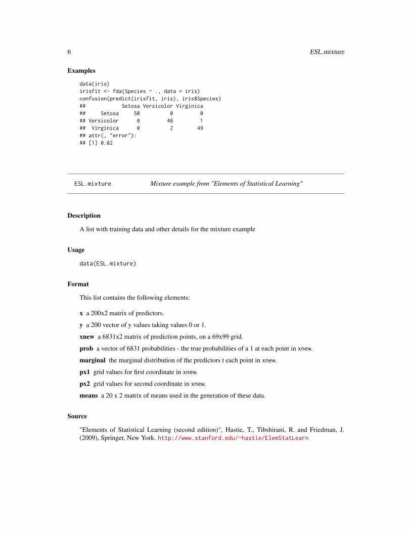
data(iris)irisfit <- fda(Species ~ ., data = iris)confusion(predict(irisfit, iris), iris$Species)## Setosa Versicolor Virginica## Setosa 50 0 0## Versicolor 0 48 1## Virginica 0 2 49## attr(, "error"):## [1] 0.02
ESL.mixture Mixture example from "Elements of Statistical Learning"
Description
A list with training data and other details for the mixture example
Usage
data(ESL.mixture)
Format
This list contains the following elements:
x a 200x2 matrix of predictors.
y a 200 vector of y values taking values 0 or 1.
xnew a 6831x2 matrix of prediction points, on a 69x99 grid.
prob a vector of 6831 probabilities - the true probabilities of a 1 at each point in xnew.
marginal the marginal distribution of the predictors t each point in xnew.
px1 grid values for first coordinate in xnew.
px2 grid values for second coordinate in xnew.
means a 20 x 2 matrix of means used in the generation of these data.
Source
"Elements of Statistical Learning (second edition)", Hastie, T., Tibshirani, R. and Friedman, J.(2009), Springer, New York. http://www.stanford.edu/~hastie/ElemStatLearn

fda 7
fda Flexible Discriminant Analysis
Description
Flexible discriminant analysis.
Usage
fda(formula, data, weights, theta, dimension, eps, method,keep.fitted, ...)
Arguments
formula of the form y~x it describes the response and the predictors. The formula can bemore complicated, such as y~log(x)+z etc (see formula for more details). Theresponse should be a factor representing the response variable, or any vector thatcan be coerced to such (such as a logical variable).
data data frame containing the variables in the formula (optional).
weights an optional vector of observation weights.
theta an optional matrix of class scores, typically with less than J-1 columns.
dimension The dimension of the solution, no greater than J-1, where J is the numberclasses. Default is J-1.
eps a threshold for small singular values for excluding discriminant variables; de-fault is .Machine$double.eps.
method regression method used in optimal scaling. Default is linear regression via thefunction polyreg, resulting in linear discriminant analysis. Other possibilitiesare mars and bruto. For Penalized Discriminant analysis gen.ridge is appro-priate.
keep.fitted a logical variable, which determines whether the (sometimes large) component"fitted.values" of the fit component of the returned fda object should bekept. The default is TRUE if n * dimension < 5000.
... additional arguments to method.
Value
an object of class "fda". Use predict to extract discriminant variables, posterior probabilities orpredicted class memberships. Other extractor functions are coef, confusion and plot.
The object has the following components:
percent.explained
the percent between-group variance explained by each dimension (relative to thetotal explained.)

8 fda
values optimal scaling regression sum-of-squares for each dimension (see reference).The usual discriminant analysis eigenvalues are given by values / (1-values),which are used to define percent.explained.
means class means in the discriminant space. These are also scaled versions of the finaltheta’s or class scores, and can be used in a subsequent call to fda (this onlymakes sense if some columns of theta are omitted—see the references).
theta.mod (internal) a class scoring matrix which allows predict to work properly.
dimension dimension of discriminant space.
prior class proportions for the training data.
fit fit object returned by method.
call the call that created this object (allowing it to be update-able)
confusion confusion matrix when classifying the training data.
The method functions are required to take arguments x and y where both can be matrices, andshould produce a matrix of fitted.values the same size as y. They can take additional argumentsweights and should all have a ... for safety sake. Any arguments to method can be passed onvia the ... argument of fda. The default method polyreg has a degree argument which allowspolynomial regression of the required total degree. See the documentation for predict.fda forfurther requirements of method. The package earth is suggested for this package as well; earth isa more detailed implementation of the mars model, and works as a method argument.
Author(s)
Trevor Hastie and Robert Tibshirani
References
“Flexible Disriminant Analysis by Optimal Scoring” by Hastie, Tibshirani and Buja, 1994, JASA,1255-1270.
“Penalized Discriminant Analysis” by Hastie, Buja and Tibshirani, 1995, Annals of Statistics, 73-102.
“Elements of Statisical Learning - Data Mining, Inference and Prediction” (2nd edition, Chapter12) by Hastie, Tibshirani and Friedman, 2009, Springer
See Also
predict.fda, plot.fda, mars, bruto, polyreg, softmax, confusion,
Examples
data(iris)irisfit <- fda(Species ~ ., data = iris)irisfit## fda(formula = Species ~ ., data = iris)#### Dimension: 2#### Percent Between-Group Variance Explained:

gen.ridge 9
## v1 v2## 99.12 100.00#### Degrees of Freedom (per dimension): 5#### Training Misclassification Error: 0.02 ( N = 150 )
confusion(irisfit, iris)## Setosa Versicolor Virginica## Setosa 50 0 0## Versicolor 0 48 1## Virginica 0 2 49## attr(, "error"):## [1] 0.02
plot(irisfit)
coef(irisfit)## [,1] [,2]## [1,] -2.126479 -6.72910343## [2,] -0.837798 0.02434685## [3,] -1.550052 2.18649663## [4,] 2.223560 -0.94138258## [5,] 2.838994 2.86801283
marsfit <- fda(Species ~ ., data = iris, method = mars)marsfit2 <- update(marsfit, degree = 2)marsfit3 <- update(marsfit, theta = marsfit$means[, 1:2])## this refits the model, using the fitted means (scaled theta's)## from marsfit to start the iterations
gen.ridge Penalized Regression
Description
Perform a penalized regression, as used in penalized discriminant analysis.
Usage
gen.ridge(x, y, weights, lambda=1, omega, df, ...)
Arguments
x, y, weights the x and y matrix and possibly a weight vector.
lambda the shrinkage penalty coefficient.
omega a penalty object; omega is the eigendecomposition of the penalty matrix, andneed not have full rank. By default, standard ridge is used.

10 glass
df an alternative way to prescribe lambda, using the notion of equivalent degreesof freedom.
... currently not used.
Value
A generalized ridge regression, where the coefficients are penalized according to omega. Seethe function definition for further details. No functions are provided for producing one dimen-sional penalty objects (omega). laplacian() creates a two-dimensional penalty object, suitablefor (small) images.
See Also
laplacian
glass Glass Identification Database
Description
The glass data frame has 214 observations and 10 variables, representing glass fragments.
Usage
data(glass)
Format
This data frame contains the following columns:
RI refractive indexNa weight percent in corresponding oxideMg weight percent in corresponding oxideAl weight percent in corresponding oxideSi weight percent in corresponding oxideK weight percent in corresponding oxideCa weight percent in corresponding oxideBa weight percent in corresponding oxideFe weight percent in corresponding oxideType Type of glass:
1 building\_windows\_float\_processed,2 building\_windows\_non\_float\_processed,3 vehicle\_windows\_float\_processed,4 vehicle\_windows\_non\_float\_processed (none in this database),5 containers,6 tableware,7 headlamps

laplacian 11
Source
P. M. Murphy and D. W. Aha (1999), UCI Repository of Machine Learning Databases, http://ftp.ics.uci.edu/pub/machine-learning-databases
laplacian create penalty object for two-dimensional smoothing.
Description
Creates a penalty matrix for use by gen.ridge for two-dimensional smoothing.
Usage
laplacian(size, compose)laplacian(size = 16, compose = FALSE)
Arguments
size dimension of the image is size x size; default is 16.
compose default is compose=FALSE, which means the penalty is returned as an eigen-decomposition. If compose=TRUE, a penalty matrix is returned.
Details
Formulas are used to construct a laplacian for smoothing a square image.
Value
If compose=FALSE, an eigen-decomposition object is returned. The vectors component is a size^2 x size^2orthogonal matrix, and the $values component is a size^2 vector of non-negative eigen-values. Ifcompose=TRUE, these are multiplied together to form a single matrix.
Author(s)
Trevor Hastie <[email protected]
References
Here we follow very closely the material on page 635 in JASA 1991 of O’Sullivan’s article ondiscretized Laplacian Smoothing
See Also
gen.ridge,fda

12 mars
mars Multivariate Adaptive Regression Splines
Description
Multivariate adaptive regression splines.
Usage
mars(x, y, w, wp, degree, nk, penalty, thresh, prune, trace.mars,forward.step, prevfit, ...)
Arguments
x a matrix containing the independent variables.
y a vector containing the response variable, or in the case of multiple responses, amatrix whose columns are the response values for each variable.
w an optional vector of observation weights (currently ignored).
wp an optional vector of response weights.
degree an optional integer specifying maximum interaction degree (default is 1).
nk an optional integer specifying the maximum number of model terms.
penalty an optional value specifying the cost per degree of freedom charge (default is 2).
thresh an optional value specifying forward stepwise stopping threshold (default is0.001).
prune an optional logical value specifying whether the model should be pruned in abackward stepwise fashion (default is TRUE).
trace.mars an optional logical value specifying whether info should be printed along theway (default is FALSE).
forward.step an optional logical value specifying whether forward stepwise process shouldbe carried out (default is TRUE).
prevfit optional data structure from previous fit. To see the effect of changing thepenalty parameter, one can use prevfit with forward.step = FALSE.
... further arguments to be passed to or from methods.
Value
An object of class "mars", which is a list with the following components:
call call used to mars.
all.terms term numbers in full model. 1 is the constant term. Remaining terms are in pairs(2 3, 4 5, and so on). all.terms indicates nonsingular set of terms.
selected.terms term numbers in selected model.
penalty the input penalty value.
mars 13
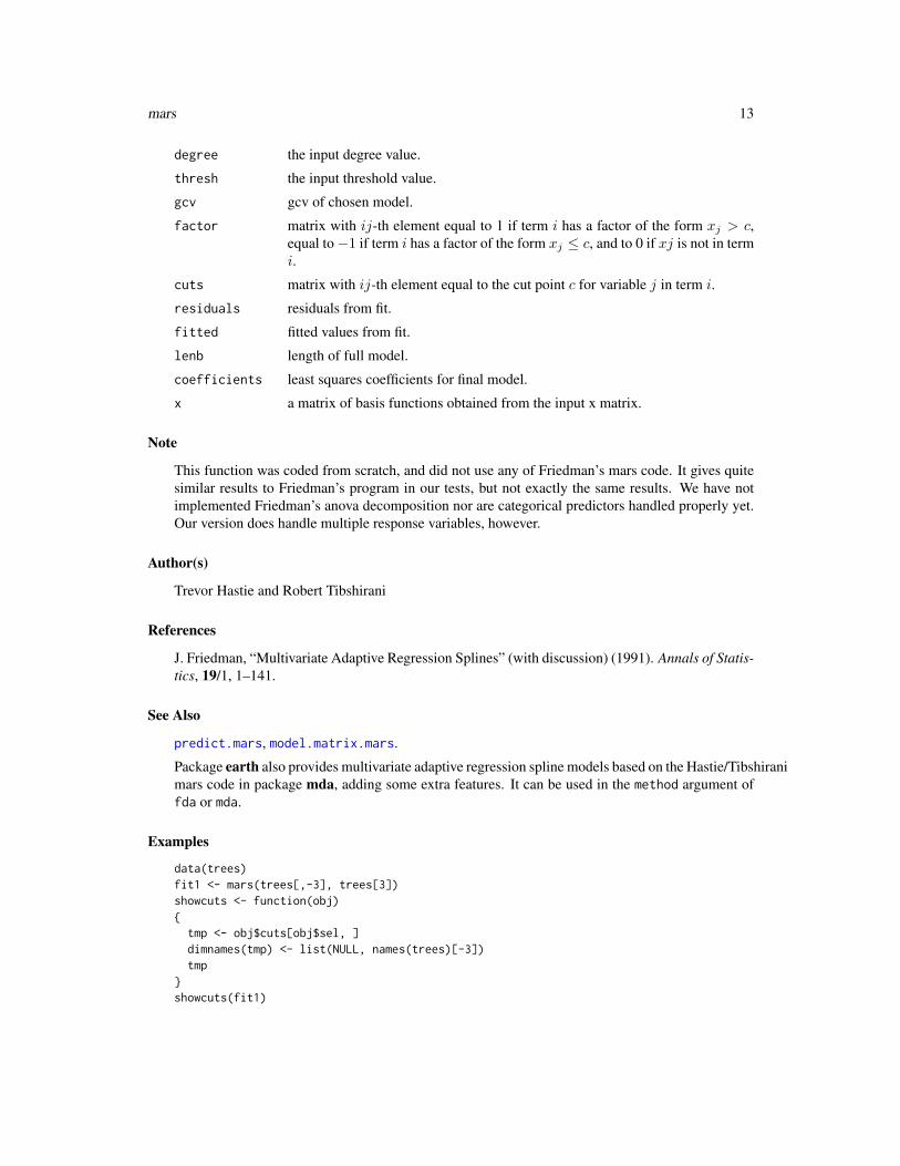
degree the input degree value.
thresh the input threshold value.
gcv gcv of chosen model.
factor matrix with ij-th element equal to 1 if term i has a factor of the form xj > c,equal to −1 if term i has a factor of the form xj ≤ c, and to 0 if xj is not in termi.
cuts matrix with ij-th element equal to the cut point c for variable j in term i.
residuals residuals from fit.
fitted fitted values from fit.
lenb length of full model.
coefficients least squares coefficients for final model.
x a matrix of basis functions obtained from the input x matrix.
Note
This function was coded from scratch, and did not use any of Friedman’s mars code. It gives quitesimilar results to Friedman’s program in our tests, but not exactly the same results. We have notimplemented Friedman’s anova decomposition nor are categorical predictors handled properly yet.Our version does handle multiple response variables, however.
Author(s)
Trevor Hastie and Robert Tibshirani
References
J. Friedman, “Multivariate Adaptive Regression Splines” (with discussion) (1991). Annals of Statis-tics, 19/1, 1–141.
See Also
predict.mars, model.matrix.mars.
Package earth also provides multivariate adaptive regression spline models based on the Hastie/Tibshiranimars code in package mda, adding some extra features. It can be used in the method argument offda or mda.
Examples
data(trees)fit1 <- mars(trees[,-3], trees[3])showcuts <- function(obj){
tmp <- obj$cuts[obj$sel, ]dimnames(tmp) <- list(NULL, names(trees)[-3])tmp
}showcuts(fit1)

14 mda
## examine the fitted functionspar(mfrow=c(1,2), pty="s")Xp <- matrix(sapply(trees[1:2], mean), nrow(trees), 2, byrow=TRUE)for(i in 1:2) {
xr <- sapply(trees, range)Xp1 <- Xp; Xp1[,i] <- seq(xr[1,i], xr[2,i], len=nrow(trees))Xf <- predict(fit1, Xp1)plot(Xp1[ ,i], Xf, xlab=names(trees)[i], ylab="", type="l")
}
mda Mixture Discriminant Analysis
Description
Mixture discriminant analysis.
Usage
mda(formula, data, subclasses, sub.df, tot.df, dimension, eps,iter, weights, method, keep.fitted, trace, ...)
Arguments
formula of the form y~x it describes the response and the predictors. The formula can bemore complicated, such as y~log(x)+z etc (see formula for more details). Theresponse should be a factor representing the response variable, or any vector thatcan be coerced to such (such as a logical variable).
data data frame containing the variables in the formula (optional).
subclasses Number of subclasses per class, default is 3. Can be a vector with a number foreach class.
sub.df If subclass centroid shrinking is performed, what is the effective degrees of free-dom of the centroids per class. Can be a scalar, in which case the same numberis used for each class, else a vector.
tot.df The total df for all the centroids can be specified rather than separately per class.
dimension The dimension of the reduced model. If we know our final model will be con-fined to a discriminant subspace (of the subclass centroids), we can specify thisin advance and have the EM algorithm operate in this subspace.
eps A numerical threshold for automatically truncating the dimension.
iter A limit on the total number of iterations, default is 5.
weights NOT observation weights! This is a special weight structure, which for eachclass assigns a weight (prior probability) to each of the observations in thatclass of belonging to one of the subclasses. The default is provided by a callto mda.start(x, g, subclasses, trace, ...) (by this time x and g are

mda 15
known). See the help for mda.start. Arguments for mda.start can be pro-vided via the ... argument to mda, and the weights argument need never beaccessed. A previously fit mda object can be supplied, in which case the fi-nal subclass responsibility weights are used for weights. This allows theiterations from a previous fit to be continued.
method regression method used in optimal scaling. Default is linear regression via thefunction polyreg, resulting in the usual mixture model. Other possibilities aremars and bruto. For penalized mixture discriminant models gen.ridge is ap-propriate.
keep.fitted a logical variable, which determines whether the (sometimes large) component"fitted.values" of the fit component of the returned mda object should bekept. The default is TRUE if n * dimension < 5000.
trace if TRUE, iteration information is printed. Note that the deviance reported is forthe posterior class likelihood, and not the full likelihood, which is used to drivethe EM algorithm under mda. In general the latter is not available.
... additional arguments to mda.start and to method.
Value
An object of class c("mda", "fda"). The most useful extractor is predict, which can make manytypes of predictions from this object. It can also be plotted, and any functions useful for fda objectswill work here too, such as confusion and coef.
The object has the following components:
percent.explained
the percent between-group variance explained by each dimension (relative to thetotal explained.)
values optimal scaling regression sum-of-squares for each dimension (see reference).
means subclass means in the discriminant space. These are also scaled versions of thefinal theta’s or class scores, and can be used in a subsequent call to mda (thisonly makes sense if some columns of theta are omitted—see the references)
theta.mod (internal) a class scoring matrix which allows predict to work properly.
dimension dimension of discriminant space.
sub.prior subclass membership priors, computed in the fit. No effort is currently spent intrying to keep these above a threshold.
prior class proportions for the training data.
fit fit object returned by method.
call the call that created this object (allowing it to be update-able).
confusion confusion matrix when classifying the training data.
weights These are the subclass membership probabilities for each member of the trainingset; see the weights argument.
assign.theta a pointer list which identifies which elements of certain lists belong to individualclasses.

16 mda
deviance The multinomial log-likelihood of the fit. Even though the full log-likelihooddrives the iterations, we cannot in general compute it because of the flexibilityof the method used. The deviance can increase with the iterations, but generallydoes not.
The method functions are required to take arguments x and y where both can be matrices, andshould produce a matrix of fitted.values the same size as y. They can take additional argumentsweights and should all have a ... for safety sake. Any arguments to method() can be passed onvia the ... argument of mda. The default method polyreg has a degree argument which allowspolynomial regression of the required total degree. See the documentation for predict.fda forfurther requirements of method. The package earth is suggested for this package as well; earth isa more detailed implementation of the mars model, and works as a method argument.
The function mda.start creates the starting weights; it takes additional arguments which can bepassed in via the ... argument to mda. See the documentation for mda.start.
Author(s)
Trevor Hastie and Robert Tibshirani
References
“Flexible Disriminant Analysis by Optimal Scoring” by Hastie, Tibshirani and Buja, 1994, JASA,1255-1270.
“Penalized Discriminant Analysis” by Hastie, Buja and Tibshirani, 1995, Annals of Statistics, 73-102
“Discriminant Analysis by Gaussian Mixtures” by Hastie and Tibshirani, 1996, JRSS-B, 155-176.
“Elements of Statisical Learning - Data Mining, Inference and Prediction” (2nd edition, Chapter12) by Hastie, Tibshirani and Friedman, 2009, Springer
See Also
predict.mda, mars, bruto, polyreg, gen.ridge, softmax, confusion
Examples
data(iris)irisfit <- mda(Species ~ ., data = iris)irisfit## Call:## mda(formula = Species ~ ., data = iris)#### Dimension: 4#### Percent Between-Group Variance Explained:## v1 v2 v3 v4## 96.02 98.55 99.90 100.00#### Degrees of Freedom (per dimension): 5#### Training Misclassification Error: 0.02 ( N = 150 )

mda.start 17
#### Deviance: 15.102
data(glass)# random sample of size 100samp <- c(1, 3, 4, 11, 12, 13, 14, 16, 17, 18, 19, 20, 27, 28, 31,
38, 42, 46, 47, 48, 49, 52, 53, 54, 55, 57, 62, 63, 64, 65,67, 68, 69, 70, 72, 73, 78, 79, 83, 84, 85, 87, 91, 92, 94,99, 100, 106, 107, 108, 111, 112, 113, 115, 118, 121, 123,124, 125, 126, 129, 131, 133, 136, 139, 142, 143, 145, 147,152, 153, 156, 159, 160, 161, 164, 165, 166, 168, 169, 171,172, 173, 174, 175, 177, 178, 181, 182, 185, 188, 189, 192,195, 197, 203, 205, 211, 212, 214)
glass.train <- glass[samp,]glass.test <- glass[-samp,]glass.mda <- mda(Type ~ ., data = glass.train)predict(glass.mda, glass.test, type="post") # abbreviations are allowedconfusion(glass.mda,glass.test)
mda.start Initialization for Mixture Discriminant Analysis
Description
Provide starting weights for the mda function which performs discriminant analysis by gaussianmixtures.
Usage
mda.start(x, g, subclasses = 3, trace.mda.start = FALSE,start.method = c("kmeans", "lvq"), tries = 5,criterion = c("misclassification", "deviance"), ...)
Arguments
x The x data, or an mda object.
g The response vector g.
subclasses number of subclasses per class, as in mda.trace.mda.start
Show results of each iteration.
start.method Either "kmeans" or "lvq". The latter requires package class (from the VRpackage bundle.
tries Number of random starts.
criterion By default, classification errors on the training data. Posterior deviance is alsoan option.
... arguments to be passed to the mda fitter when using posterior deviance.

18 model.matrix.mars
Value
A list of weight matrices, one for each class.
model.matrix.mars Produce a Design Matrix from a ‘mars’ Object
Description
Produce a design matrix from a ‘mars’ object.
Usage
## S3 method for class 'mars'model.matrix(object, x, which, full = FALSE, ...)
Arguments
object a mars object.
x optional argument; if supplied, the mars basis functions are evaluated at thesenew observations.
which which columns should be used. The default is to use the columns described bythe component selected.terms on object.
full if TRUE the entire set of columns are selected, even redundant ones. This is usedfor updating a mars fit.
... further arguments to be passed from or to methods.
Value
A model matrix corresponding to the selected columns.
See Also
mars, predict.mars

mspline 19
mspline Vector Smoothing Spline
Description
Fit a smoothing spline to a matrix of responses, single x.
Usage
mspline(x, y, w, df = 5, lambda, thresh = 1e-04, ...)
Arguments
x x variable (numeric vector).y response matrix.w optional weight vector, defaults to a vector of ones.df requested degrees of freedom, as in smooth.spline.lambda can provide penalty instead of df.thresh convergence threshold for df inversion (to lambda).... holdall for other arguments.
Details
This function is based on the ingredients of smooth.spline, and allows for simultaneous smoothingof multiple responses
Value
A list is returned, with a number of components, only some of which are of interest. These are
lambda The value of lambda used (in case df was supplied)df The df used (in case lambda was supplied)s A matrix like y of smoothed responseslev Self influences (diagonal of smoother matrix)
Author(s)
Trevor Hastie
See Also
smooth.spline
Examples
x=rnorm(100)y=matrix(rnorm(100*10),100,10)fit=mspline(x,y,df=5)

20 plot.fda
plot.fda Plot for Flexible Discriminant Analysis
Description
Plot in discriminant (canonical) coordinates a fda or (by inheritance) a mda object.
Usage
## S3 method for class 'fda'plot(x, data, coords, group, colors, pch, mcolors, mpch, pcex, mcex, ...)
Arguments
x an object of class "fda".data the data to plot in the discriminant coordinates. If group="true", then data
should be a data frame with the same variables that were used in the fit. Ifgroup="predicted", data need not contain the response variable, and can infact be the correctly-sized "x" matrix.
coords vector of coordinates to plot, with default coords="c(1,2)". All pairs of plotsare produced.
group if group="true" (the default), each point is color and symbol coded accord-ing to the response in data. If group="predicted", the class of each point ispredicted from the model, and used instead.
colors a vector of colors to be used in the plotting.pch a vector of plotting characters.mcolors a vector of colors for the class centroids; default is colors.mpch a vector of plotting characters for the centroids.pcex character expansion factor for the points; defualt is pcex="0.5".mcex character expansion factor for the centroids; defualt is pcex="2.5".... further arguments to be passed to or from methods.
See Also
fda, mda, predict.fda
Examples
data(iris)irisfit <- fda(Species ~ ., data = iris)plot(irisfit)data(ESL.mixture)## Not a data framemixture.train=ESL.mixture[c("x","y")]mixfit=mda(y~x, data=mixture.train)plot(mixfit, mixture.train)plot(mixfit, data=ESL.mixture$xnew, group="pred")

polyreg 21
polyreg Polynomial Regression
Description
Simple minded polynomial regression.
Usage
polyreg(x, y, w, degree = 1, monomial = FALSE, ...)
Arguments
x predictor matrix.
y response matrix.
w optional (positive) weights.
degree total degree of polynomial basis (default is 1).
monomial If TRUE a monomial basis is used (no cross terms). Default is FALSE.
... currently not used.
Value
A polynomial regression fit, containing the essential ingredients for its predict method.
predict.bruto Predict method for BRUTO Objects
Description
Predicted values based on ‘bruto’ additive spline models which are fit by adaptive backfitting.
Usage
## S3 method for class 'bruto'predict(object, newdata, type=c("fitted", "terms"), ...)
Arguments
object a fitted bruto object
newdata values at which predictions are to be made.
type if type is "fitted", the fitted values are returned. If type is "terms", a list offitted terms is returned, each with an x and y component. These can be used toshow the fitted functions.
... further arguments to be passed to or from methods.

22 predict.fda
Value
Either a fit matrix or a list of fitted terms.
See Also
bruto, predict
Examples
data(trees)fit1 <- bruto(trees[,-3], trees[3])fitted.terms <- predict(fit1, as.matrix(trees[,-3]), type = "terms")par(mfrow=c(1,2), pty="s")for(tt in fitted.terms) plot(tt, type="l")
predict.fda Classify by Flexible Discriminant Analysis
Description
Classify observations in conjunction with fda.
Usage
## S3 method for class 'fda'predict(object, newdata, type, prior, dimension, ...)
Arguments
object an object of class "fda".
newdata new data at which to make predictions. If missing, the training data is used.
type kind of predictions: type = "class" (default) produces a fitted factor, type = "variates"produces a matrix of discriminant (canonical) variables, type = "posterior"produces a matrix of posterior probabilities (based on a gaussian assumption),and type = "hierarchical" produces the predicted class in sequence formodels of all dimensions.
prior the prior probability vector for each class; the default is the training sampleproportions.
dimension the dimension of the space to be used, no larger than the dimension componentof object.
... further arguments to be passed to or from methods.
Value
An appropriate object depending on type. object has a component fit which is regression fitproduced by the method argument to fda. There should be a predict method for this object whichis invoked. This method should itself take as input object and optionally newdata.

predict.mars 23
See Also
fda, mars, bruto, polyreg, softmax, confusion
Examples
data(iris)irisfit <- fda(Species ~ ., data = iris)irisfit## Call:## fda(x = iris$x, g = iris$g)#### Dimension: 2#### Percent Between-Group Variance Explained:## v1 v2## 99.12 100confusion(predict(irisfit, iris), iris$Species)## Setosa Versicolor Virginica## Setosa 50 0 0## Versicolor 0 48 1## Virginica 0 2 49## attr(, "error"):## [1] 0.02
predict.mars Predict method for MARS Objects
Description
Predicted values based on ‘mars’ multivariate adaptive regression spline models.
Usage
## S3 method for class 'mars'predict(object, newdata, ...)
Arguments
object an object of class "mars".newdata values at which predictions are to be made.... further arguments to be passed to or from methods.
Value
the fitted values.
See Also
mars, predict, model.matrix.mars
24 predict.mda
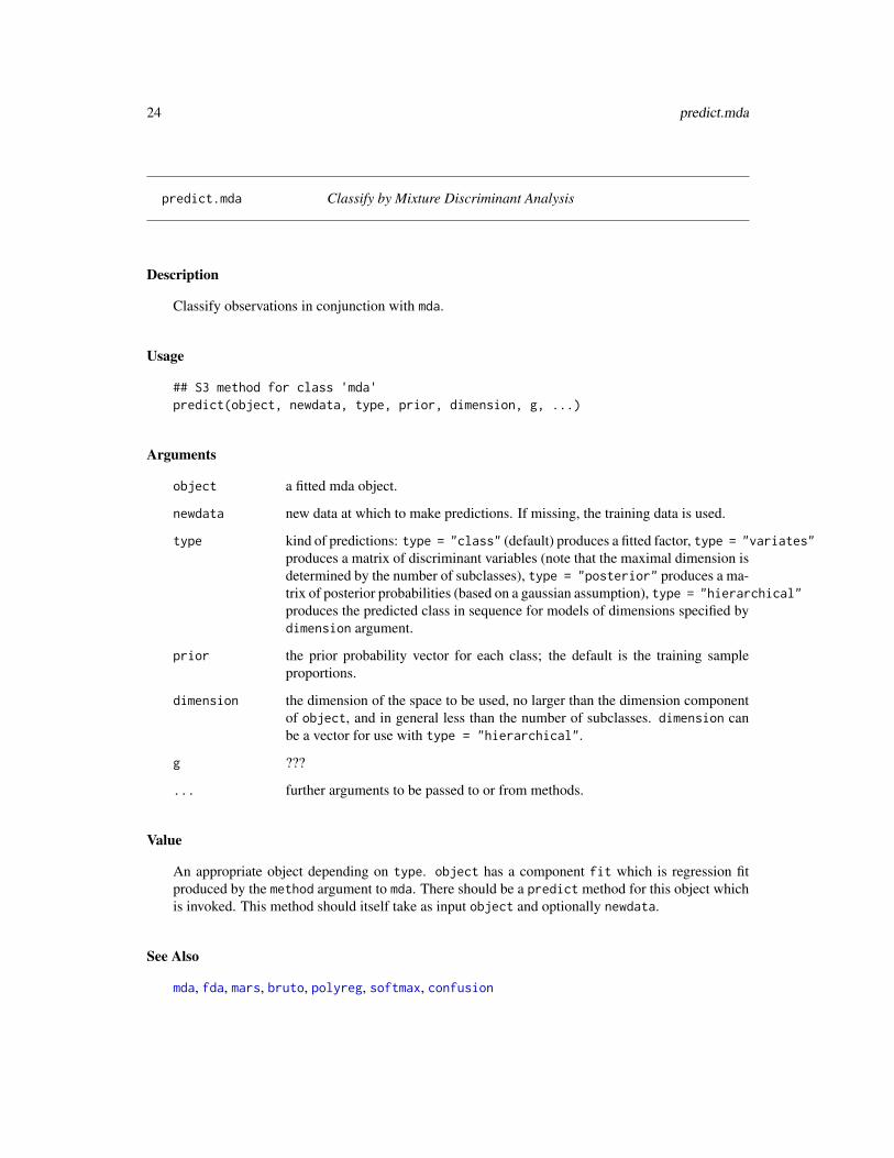
predict.mda Classify by Mixture Discriminant Analysis
Description
Classify observations in conjunction with mda.
Usage
## S3 method for class 'mda'predict(object, newdata, type, prior, dimension, g, ...)
Arguments
object a fitted mda object.
newdata new data at which to make predictions. If missing, the training data is used.
type kind of predictions: type = "class" (default) produces a fitted factor, type = "variates"produces a matrix of discriminant variables (note that the maximal dimension isdetermined by the number of subclasses), type = "posterior" produces a ma-trix of posterior probabilities (based on a gaussian assumption), type = "hierarchical"produces the predicted class in sequence for models of dimensions specified bydimension argument.
prior the prior probability vector for each class; the default is the training sampleproportions.
dimension the dimension of the space to be used, no larger than the dimension componentof object, and in general less than the number of subclasses. dimension canbe a vector for use with type = "hierarchical".
g ???
... further arguments to be passed to or from methods.
Value
An appropriate object depending on type. object has a component fit which is regression fitproduced by the method argument to mda. There should be a predict method for this object whichis invoked. This method should itself take as input object and optionally newdata.
See Also
mda, fda, mars, bruto, polyreg, softmax, confusion

softmax 25
Examples
data(glass)samp <- sample(1:nrow(glass), 100)glass.train <- glass[samp,]glass.test <- glass[-samp,]glass.mda <- mda(Type ~ ., data = glass.train)predict(glass.mda, glass.test, type = "post") # abbreviations are allowedconfusion(glass.mda, glass.test)
softmax Find the Maximum in Each Row of a Matrix
Description
Find the maximum in each row of a matrix.
Usage
softmax(x, gap = FALSE)
Arguments
x a numeric matrix.
gap if TRUE, the difference between the largest and next largest column is returned.
Value
A factor with levels the column labels of x and values the columns corresponding to the maximumcolumn. If gap = TRUE a list is returned, the second component of which is the difference betweenthe largest and next largest column of x.
See Also
predict.fda, confusion, fda mda
Examples
data(iris)irisfit <- fda(Species ~ ., data = iris)posteriors <- predict(irisfit, type = "post")confusion(softmax(posteriors), iris[, "Species"])

Index
∗Topic categoryconfusion, 5
∗Topic classifcoef.fda, 4fda, 7mda, 14mda.start, 17plot.fda, 20predict.fda, 22predict.mda, 24
∗Topic datasetsESL.mixture, 6glass, 10
∗Topic modelsmodel.matrix.mars, 18
∗Topic regressiongen.ridge, 9laplacian, 11polyreg, 21
∗Topic smoothbruto, 2mars, 12predict.bruto, 21predict.mars, 23
∗Topic utilitiessoftmax, 25
bruto, 2, 4, 8, 16, 22–24
coef.fda, 4coef.mda (coef.fda), 4confusion, 4, 5, 8, 16, 23–25
ESL.mixture, 6
fda, 5, 7, 11, 20, 23–25formula, 7, 14
gen.ridge, 9, 11, 16glass, 10
laplacian, 10, 11
mars, 4, 8, 12, 16, 18, 23, 24mda, 14, 20, 24, 25mda.start, 15, 17model.matrix.mars, 13, 18, 23mspline, 19
plot.fda, 4, 8, 20polyreg, 4, 8, 16, 21, 23, 24predict, 22, 23predict.bruto, 3, 21predict.fda, 4, 5, 8, 16, 20, 22, 25predict.gen.ridge (gen.ridge), 9predict.mars, 13, 18, 23predict.mda, 16, 24predict.polyreg (polyreg), 21print.fda (fda), 7print.mda (mda), 14
smooth.spline, 19softmax, 4, 8, 16, 23, 24, 25
26