package ‘lctools’ - r · package ‘lctools ’ april 23, 2019 ... gression methods including...

Package ‘lctools’April 23, 2019

Version 0.2-7

Date 2019-05-22

Type Package

Title Local Correlation, Spatial Inequalities, Geographically WeightedRegression and Other Tools

Author Stamatis Kalogirou [aut, cre]

Maintainer Stamatis Kalogirou <[email protected]>

Depends R (>= 3.5.0), reshape (>= 0.8.8), weights (>= 1.0), pscl (>=1.5.2), MASS (>= 7.3-51.3)

Description Provides researchers and educators with easy-to-learn user friendly tools for calculatingkey spatial statistics and to apply simple as well as advanced methods of spatial analy-sis in real data.These include: Local Pearson and Geographically Weighted Pearson Correlation Coefficients,Spatial Inequality Measures (Gini, Spatial Gini, LQ, Focal LQ), Spatial Autocorrelation(Global and Local Moran's I), several Geographically Weighted Regression techniques and otherSpatial Analysis tools (other geographically weighted statistics). This package also con-tains functions formeasuring the significance of each statistic calculated, mainly based on Monte Carlo simulations.

License GPL (>= 2)

VignetteBuilder knitr

URL http://lctools.science/

Suggests knitr, sp

NeedsCompilation no

Repository CRAN

Date/Publication 2019-04-23 05:50:03 UTC

R topics documented:lctools-package . . . . . . . . . . . . . . . . . . . . . . . . . . . . . . . . . . . . . . . 2acc . . . . . . . . . . . . . . . . . . . . . . . . . . . . . . . . . . . . . . . . . . . . . . 4FLQ . . . . . . . . . . . . . . . . . . . . . . . . . . . . . . . . . . . . . . . . . . . . . 5

1

http://lctools.science/

2 lctools-package

GR.Municipalities . . . . . . . . . . . . . . . . . . . . . . . . . . . . . . . . . . . . . . 6gw.glm . . . . . . . . . . . . . . . . . . . . . . . . . . . . . . . . . . . . . . . . . . . 8gw.glm.bw . . . . . . . . . . . . . . . . . . . . . . . . . . . . . . . . . . . . . . . . . . 10gw.glm.cv . . . . . . . . . . . . . . . . . . . . . . . . . . . . . . . . . . . . . . . . . . 12gw.glm.light . . . . . . . . . . . . . . . . . . . . . . . . . . . . . . . . . . . . . . . . . 13gw.glm.mc.test . . . . . . . . . . . . . . . . . . . . . . . . . . . . . . . . . . . . . . . 14gw.zi . . . . . . . . . . . . . . . . . . . . . . . . . . . . . . . . . . . . . . . . . . . . . 16gw.zi.bw . . . . . . . . . . . . . . . . . . . . . . . . . . . . . . . . . . . . . . . . . . . 18gw.zi.cv . . . . . . . . . . . . . . . . . . . . . . . . . . . . . . . . . . . . . . . . . . . 20gw.zi.light . . . . . . . . . . . . . . . . . . . . . . . . . . . . . . . . . . . . . . . . . . 21gw.zi.mc.test . . . . . . . . . . . . . . . . . . . . . . . . . . . . . . . . . . . . . . . . 23gwr . . . . . . . . . . . . . . . . . . . . . . . . . . . . . . . . . . . . . . . . . . . . . 25gwr.bw . . . . . . . . . . . . . . . . . . . . . . . . . . . . . . . . . . . . . . . . . . . 27gwr.cv . . . . . . . . . . . . . . . . . . . . . . . . . . . . . . . . . . . . . . . . . . . . 29gw_variable . . . . . . . . . . . . . . . . . . . . . . . . . . . . . . . . . . . . . . . . . 30l.moransI . . . . . . . . . . . . . . . . . . . . . . . . . . . . . . . . . . . . . . . . . . 31lat2w . . . . . . . . . . . . . . . . . . . . . . . . . . . . . . . . . . . . . . . . . . . . 33lcorrel . . . . . . . . . . . . . . . . . . . . . . . . . . . . . . . . . . . . . . . . . . . . 34mc.lcorrel . . . . . . . . . . . . . . . . . . . . . . . . . . . . . . . . . . . . . . . . . . 36mc.spGini . . . . . . . . . . . . . . . . . . . . . . . . . . . . . . . . . . . . . . . . . . 38moransI . . . . . . . . . . . . . . . . . . . . . . . . . . . . . . . . . . . . . . . . . . . 40moransI.v . . . . . . . . . . . . . . . . . . . . . . . . . . . . . . . . . . . . . . . . . . 42moransI.w . . . . . . . . . . . . . . . . . . . . . . . . . . . . . . . . . . . . . . . . . . 44random.test.data . . . . . . . . . . . . . . . . . . . . . . . . . . . . . . . . . . . . . . . 46spg.sim.test . . . . . . . . . . . . . . . . . . . . . . . . . . . . . . . . . . . . . . . . . 47spGini . . . . . . . . . . . . . . . . . . . . . . . . . . . . . . . . . . . . . . . . . . . . 49spGini.w . . . . . . . . . . . . . . . . . . . . . . . . . . . . . . . . . . . . . . . . . . . 50VotesGR . . . . . . . . . . . . . . . . . . . . . . . . . . . . . . . . . . . . . . . . . . . 51w.matrix . . . . . . . . . . . . . . . . . . . . . . . . . . . . . . . . . . . . . . . . . . . 52

Index 54

lctools-package Local Correlation, Spatial Inequalities, Spatial Regression and OtherTools

Description

The main purpose of lctools is to assist spatial analysis researchers and educators to use simple,yet powerful, transparent and user friendly tools for calculating key spatial statistics and fitting spa-tial models. lctools was originally created to help testing the existence of local multi-collinearityamong the explanatory variables of local regression models. The main function (lcorrel) allows forthe computation of Local Pearson and Geographically Weighted Pearson Correlation Coefficientsand their significance. However, the latter could also be used for examining the existence of localassociation between pairs of variables. As spatial analysis techniques develop, this package hasother spatial statistical tools: the spatial decomposition of the Gini coefficient, the spatial/Focal LQ,global and local Moran’s I and tools that help computing variables for Spatial Interaction Models.

lctools-package 3

Since the version 0.2-4, lctools allows for the application of various Geographically Weighted Re-gression methods including the Geographically Weighted Zero Inflated Poisson Regression recentlyproposed in the literature (Kalogirou, 2016). This package also contains functions for measuringthe significance level for each statistic calculated. The latter mainly refers to Monte Carlo simula-tions. The package comes with two datasets one of which is a spatial data frame that refers to theMunicipalities in Greece.

Details

Package: lctoolsType: PackageVersion: 0.2-7Date: 2018-05-20License: GPL (>= 2)

Note

Acknowledgement: I am grateful to the University of Luxembourg and would like to personallythank Ass. Professor Geoffrey Caruso, Professor Markus Hesse and Professor Christian Schulzfor their support during my research visit at the Institute of Geography and Spatial Planning (Sept.2013 - Feb. 2014) where this package was originally developed.

Author(s)

Stamatis Kalogirou

Maintainer: Stamatis Kalogirou <[email protected]>

References

Hope, A.C.A. (1968) A Simplified Monte Carlo Significance Test Procedure, Journal of the RoyalStatistical Society. Series B (Methodological), 30 (3), pp. 582 - 598.

Kalogirou, S. (2003) The Statistical Analysis and Modelling of Internal Migration Flows withinEngland and Wales, PhD Thesis, School of Geography, Politics and Sociology, University of New-castle upon Tyne, UK. http://gisc.gr/?mdocs-file=1245&mdocs-url=false

Kalogirou, S. (2012) Testing local versions of correlation coefficients, Review of Regional Research- Jahrbuch fur Regionalwissenschaft, 32(1), pp. 45-61, doi: 10.1007/s10037-011-0061-y. http://link.springer.com/article/10.1007/s10037-011-0061-y

Kalogirou, S. (2013) Testing geographically weighted multicollinearity diagnostics, GISRUK 2013,Department of Geography and Planning, School of Environmental Sciences, University of Liver-pool, Liverpool, UK, 3-5 April 2013. http://gisc.gr/?mdocs-file=1140&mdocs-url=false

Kalogirou, S. (2015) Spatial Analysis: Methodology and Applications with R. [ebook] Athens:Hellenic Academic Libraries Link. ISBN: 978-960-603-285-1 (in Greek). https://repository.kallipos.gr/handle/11419/5029?locale=en

http://gisc.gr/?mdocs-file=1245&mdocs-url=false

http://link.springer.com/article/10.1007/s10037-011-0061-y



https://repository.kallipos.gr/handle/11419/5029?locale=en


4 acc

Kalogirou, S. (2016) Destination Choice of Athenians: an application of geographically weightedversions of standard and zero inflated Poisson spatial interaction models, Geographical Analy-sis, 48(2),pp. 191-230. DOI: 10.1111/gean.12092 http://onlinelibrary.wiley.com/doi/10.1111/gean.12092/abstract

Rey, S.J., Smith, R.J. (2013) A spatial decomposition of the Gini coefficient, Letters in Spatial andResource Sciences, 6 (2), pp. 55-70.

acc Spatial Interaction Models: Destination Accessibility

Description

Destination accessibility or centrality or competition is a variable that when added to a destinationchoice model forms the competing destinations choice model. A simple formula for this variableis:

Aj = Σ(Wm/Djm)|m <> j

where Aj is the potential accessibility of destination j to all other potential destinations m, Wm isa weight generally measured by population, and Djm is the distance between j and m.

Usage

acc(X, Y, Pop, Power=1)

Arguments

X a numeric vector of x coordinates

Y a numeric vector of y coordinates

Pop a numeric vector of the weights, usually a population variable

Power a power of the distance; default is 1

Value

AccMeasure a single column numeric matrix of accessibility scores

Note

X,Y should be Cartesian coordinates for the distances to be measured in meters. In the sampledataset GR.Municipalities the projection used is the EPSG:2100 (GGRS87 / Greek Grid)

Author(s)

Stamatis Kalogirou <[email protected]>

http://onlinelibrary.wiley.com/doi/10.1111/gean.12092/abstract


FLQ 5

References



Examples

data(GR.Municipalities)attr<-GR.Municipalities@dataaMeasure<-acc(attr$X[1:100], attr$Y[1:100],attr$PopTot01[1:100],1)

FLQ Focal Location Quotient

Description

This is the implementation of the Focal Location Quotients proposed by Cromley and Hanink(2012). The function calculates the standard LQ and the Focal LQ based on a kernel of nearestneighbours. Two weighted schemes are currently supported: binary and bi-square weights for afixed number of nearest neighbours set by the user.

Usage

FLQ(Coords, Bandwidth, e, E, Denominator, WType = "Bi-square")

Arguments

Coords a numeric matrix or vector or dataframe of two columns giving the X,Y co-ordinates of the observations (data points or geometric / population weightedcentroids)

Bandwidth a positive value that defines the number of nearest neighbours for the calculationof the weights

e a numeric vector of a variable e_i as in the nominator of the Equation 1 (Crom-ley and Hanink, 2012) referring to the employment in a given sector for eachlocation

E a numeric vector of a variable E_i as in the nominator of the Equation 1 (Crom-ley and Hanink, 2012) referring to the total employment in a given sector foreach location

Denominator a ratio as in the denominator (e/E) of the Equation 1 (Cromley and Hanink,2012), where e and E are total employment in the given sector and overall em-ployment in the reference economy, respectively.




6 GR.Municipalities

WType string giving the weighting scheme used to compute the weights matrix. Optionsare: "Binary", "Bi-square". Default is "Bi-square".Binary: weight = 1 for distances less than or equal to the distance of the furthestneighbour (H), 0 otherwise;Bi-square: weight = (1-(ndist/H)^2)^2 for distances less than or equal to H, 0otherwise

Value

FLQ returns a list of 2 vectors:

LQ A numeric vector with the Location Quotient values

FLQ A numeric vector with the Focal Location Quotient values

Author(s)


References

Cromley, R. G. and Hanink, D. M. (2012), Focal Location Quotients: Specification and Application,Geographical Analysis, 44 (4), pp. 398-410. doi: 10.1111/j.1538-4632.2012.00852.x


Examples

data(VotesGR)res<-FLQ(cbind(VotesGR$X, VotesGR$Y),4,VotesGR$NDJune12,VotesGR$AllJune12,0.2966)boxplot(res)

GR.Municipalities Municipalities in Greece in 2011

Description

Municipality boundaries and socioeconomic variables aggregated to the new local authority geog-raphy (Programme Kallikratis).

Usage

data(GR.Municipalities)



GR.Municipalities 7

Format

A data frame with 325 observations on the following 14 variables.

OBJECTID a numeric vector of area IDs

X a numeric vector of x coordinates

Y a numeric vector of y coordinates

Name a character vector of municipality names (in greeklish)

CodeELSTAT a character vector of municipality codes to link with data from the Hellenic StatisticalAuthority (EL.STAT.)

PopM01 a numeric vector of the total population for males in 2001 (Census)

PopF01 a numeric vector of the total population for females in 2001 (Census)

PopTot01 a numeric vector of the total population in 2001 (Census)

UnemrM01 a numeric vector of unemployment rate for males in 2001 (Census)

UnemrF01 a numeric vector of unemployment rate for females in 2001 (Census)

UnemrT01 a numeric vector of total unemployment rate in 2001 (Census)

PrSect01 a numeric vector of the proportion of economically active working in the primary finan-cial sector (mainly agriculture; fishery; and forestry in 2001 (Census))

Foreig01 a numeric vector of proportion of people who do not have the Greek citizenship in 2001(Census)

Income01 a numeric vector of mean recorded household income (in Euros) earned in 2001 anddeclared in 2002 tax forms

Details

The X,Y coordinates refer to the geometric centroids of the new 325 Municipalities in Greece(Programme Kallikratis) in 2011. The boundary data of the original shapefile have been simplifiedto reduce its detail and size. The polygon referring to Mount Athos has been removed as there is nodata available for this politically autonomous area of Greece.

Source

The shapefile of the corresponding polygons is available from the Hellenic Statistical Authority(EL.STAT.) at http://www.statistics.gr/el/digital-cartographical-data. The popula-tion, employment, citizenship and employment sector data is available from the Hellenic StatisticalAuthority (EL.STAT.) at http://www.statistics.gr/en/home but were aggregated to the newmunicipalities by the author. The income data are available from the General Secretariat of Infor-mation Systems in Greece at http://www.gsis.gr/ at the postcode level of geography and wereaggregated to the new municipalities by the author.

References

Kalogirou, S., and Hatzichristos, T. (2007). A spatial modelling framework for income estimation.Spatial Economic Analysis, 2(3), 297-316. http://www.tandfonline.com/doi/abs/10.1080/17421770701576921

http://www.statistics.gr/el/digital-cartographical-data

http://www.statistics.gr/en/home

http://www.gsis.gr/

http://www.tandfonline.com/doi/abs/10.1080/17421770701576921

http://www.tandfonline.com/doi/abs/10.1080/17421770701576921

8 gw.glm

Kalogirou, S. (2010). Spatial inequalities in income and post-graduate educational attainment inGreece. Journal of Maps, 6(1), 393-400.http://www.tandfonline.com/doi/abs/10.4113/jom.2010.1095


Examples

data(GR.Municipalities)boxplot(GR.Municipalities@data$Income01)hist(GR.Municipalities@data$PrSect01)

gw.glm Generalised Geographically Weighted Regression (GGWR)

Description

This function allows for the calibration of a local model using a Generalised Geographically WeightedRegression (GGWR). At the moment this function has been coded in order to fit a GeographicallyWeighted Poisson Regression (GWPR) model.

Usage

gw.glm(formula, family, dframe, bw, kernel, coords)

Arguments

formula the local model to be fitted using the same syntax used in the glm function in R.This is a sting that is passed to the sub-models’ glm function. For more detailslook at the class formula.

family a description of the error distribution and link function to be used in the localmodel as in the glm function. Currently the only option tested is "poisson".

dframe a numeric data frame of at least two suitable variables (one dependent and oneindependent)

bw a positive number that may be an integer in the case of an "adaptive kernel" ora real in the case of a "fixed kernel". In the first case the integer denotes thenumber of nearest neighbours, whereas in the latter case the real number refersto the bandwidth (in meters if the coordinates provided are Cartesian). Thisargument can be also the result of a bandwidth selection algorithm such as thoseavailable in the function gw.glm.bw

kernel the kernel to be used in the regression. Options are "adaptive" or "fixed". Theweighting scheme used here is defined by the bi-square function (weight =(1− (ndist/H)2)2 for distances less than or equal to H , 0 otherwise)

coords a numeric matrix or data frame of two columns giving the X,Y coordinates ofthe observations

http://www.tandfonline.com/doi/abs/10.4113/jom.2010.1095

http://www.tandfonline.com/doi/abs/10.4113/jom.2010.1095


gw.glm 9

Details

The Generalised Geographically Weighted Regression is a method recently proposed building onthe simple GWR. It allows for the investigation of the existence of spatial non-stationarity in therelationship between a dependent and a set of independent variables in the cases in which the de-pendent function does not follow a normal distribution. This is possible by fitting a sub-model foreach observation is space, taking into account the neighbour observations weighted by distance. Adetailed description of the Geographically Weighted Poisson Regression currently supported herealong with examples from internal migration modelling can be found in two publication by Kalo-girou (2003, 2015). The difference of this functions to existing ones is that each time the sub-datasetis selected and the sub-model is fitted using R’s glm function instead of fitting the complete localmodel with matrix algebra. The latter approach may be faster but more prone to rounding error andcode crashing.

Value

GGLM_LEst a numeric data frame with the local intercepts and the local parameter estimatesfor each independent variable in the model’s formula.

GGLM_LPvalues a numeric data frame with the local p-value for the local intercepts and the localparameter estimates for each independent variable in the model’s formula.

GGLM_GofFit a numeric data frame with residuals and local goodness of fit statistics (AIC,Deviance)

Warning

Large datasets may take long to calibrate.

Note

This function is under development. There should be improvements in future versions of the pack-age lctools. Any suggestion is welcome!

Author(s)


References



See Also

gw.glm.bw gw.zi gwr




10 gw.glm.bw

Examples

RDF <- random.test.data(12,12,3,"poisson")gwpr <- gw.glm(dep ~ X1 + X2, "poisson", RDF, 50, kernel = 'adaptive', cbind(RDF$X,RDF$Y))

gw.glm.bw Optimal bandwidth estimation for Generalised GeographicallyWeighted Regression (GGWR)

Description

This function helps choosing the optimal bandwidth for the Generalised Geographically WeightedRegression (GGWR). At the moment the latter refers to the Geographically Weighted Poisson Re-gression (GWPR).

Usage

gw.glm.bw(formula, family, dframe, coords, kernel, algorithm="exhaustive",optim.method="Nelder-Mead", b.min=NULL, b.max=NULL, step=NULL)

Arguments





kernel the kernel to be used in the regression. Options are "adaptive" or "fixed". Theweighting scheme used here is defined by the bi-square function (weight = (1-(ndist/H)^2)^2for distances less than or equal to H, 0 otherwise)

algorithm a character argument that specifies whether the function will use an exhaustiveor a heuristic algorithm. In the first case all possible bandwidths within arange are being tested. In the second case the optim function is being usedallowing for the choice of various optimisation methods (such as Brent or BFGS)that may find a global or local optimum. The default algorithm is "exhaustive"

optim.method the optimisation method to be used. A detailed discussion is available at the ’De-tails’ section of the function optim (stats). Example methods are "Nelder-Mead","Brent", "BFGS", "CG" and "L-BFGS-B". The default method is "Nelder-Mead".

b.min the minimum bandwidth. This is important for both algorithms. In the case ofthe exhaustive algorithm it sets the lower boundary for the range in which thefunction will compute the CV score for each possible bandwidth. In the caseof the heuristic algorithm it provides the initial value for the bandwidth to be

gw.glm.bw 11

optimised which is very important. In the latter case b.min and b.max should beprovided if the optimisation method "L-BFGS-B" or "Brent" has been selected.

b.max the maximum bandwidth. This is important for both algorithms. In the caseof the exhaustive algorithm it sets the upper boundary for the range in whichthe function will compute the CV score for each possible bandwidth. In thecase of the heuristic algorithm b.max and b.min should be provided if theoptimisation method "L-BFGS-B" or "Brent" has been selected.

step this numeric argument is used only in the case of a fixed kernel indicating theincrement of the sequence of bandwidths in between the b.min and the b.max.In the case of the adaptive kernel the increment is 1 neighbour.

Details

Please carefully read the function optim(stats) when using a heuristic algorithm.

Value

bw The optimal bandwidth (fixed or adaptive)

CV The corresponding Cross Validation score for the optimal bandwidth

CVs Available only in the case of the exhaustive algorithm. This is a numericmatrix in which the first column refers to the bandwidth in test and the secondto the corresponding CV score.

Warning

Large datasets increase the processing time.

Note

Please select the optimisation algorithm carefully. This function needs further testing. Please reportany bugs!

Author(s)


References


See Also

gwr



12 gw.glm.cv

Examples

RDF <- random.test.data(12,12,3,"poisson")gwpr.bw <-gw.glm.bw(dep ~ X1 + X2, "poisson", RDF, cbind(RDF$X,RDF$Y),

kernel = 'adaptive', b.min = 48, b.max=50)

gw.glm.cv A specific version of the function gw.glm

Description

A specific version of the function gw.glm returning only the leave-one-out Cross Validation (CV)score. gw.glm.cv exludes the observation for which a sub-model fits.

Usage

gw.glm.cv(bw, formula, family, dframe, obs, kernel, dmatrix)

Arguments

bw a positive number that may be an integer in the case of an "adaptive kernel" ora real in the case of a "fixed kernel". In the first case the integer denotes thenumber of nearest neighbours, whereas in the latter case the real number refersto the bandwidth (in meters if the coordinates provided are Cartesian).




obs number of observations in the global dataset


dmatrix eucledian distance matrix between the observations

Details

Only used by gw.glm.bw

Value

Leave-one-out Cross Validation (CV) score

gw.glm.light 13

Author(s)


References



See Also

gw.glm.bw

gw.glm.light A light version of the Generalised Geographically Weighted Regres-sion (GGWR)

Description

This function allows for the calibration of a local model using the Generalised GeographicallyWeighted Regression (GGWR) but reports and returns fewer results compared to the functiongw.glm.

Usage

gw.glm.light(formula, family, dframe, bw, kernel, coords)

Arguments








14 gw.glm.mc.test



Details

For more details look at the function gw.glm. gw.glm.light is only used by the function gw.glm.mc.testin order to asses if the local parameter estimates of the Generalised Geographically Weighted Re-gression (GGWR) exhibit a significant spatial variation.

Value

A numeric data frame with the local intercepts and the local parameter estimates for each indepen-dent variable in the model’s formula.

Author(s)


References


See Also

gw.glm, gw.glm.mc.test

gw.glm.mc.test Significance test for the spatial variation of the Generalised Geo-graphically Weighted Regression local parameter estimates

Description

This function provides one approach for testing the significance of the spatial variation of the lo-cal parameter estimates resulted in by fitting a Generalised Geographically Weighted Regression(GGWR) model. The approach consists of a Monte Carlo simulation according to which: a) thedata are spatially reallocated in a random way; b) GGWR models fit for the original and simulatedspatial data sets; c) the variance of each variable for the original and simulated sets is then calcu-lated; d) a pseudo p-value for each variable V is calculated as p = (1+C)/(1+M) where C is thenumber of cases in which the simulated data sets generated variances of the local parameter esti-mates of the variable V that were as extreme as the observed local parameter estimates variance ofthe variable in question and M is the number of permutations. If p <= 0.05 it can be argued thatthe spatial variation of the local parameters estimates for a variable V is statistically significant. Forthis approach, a minimum of 19 simulations is required.



gw.glm.mc.test 15

Usage

gw.glm.mc.test(Nsim = 19, formula, family, dframe, bw, kernel, coords)

Arguments

Nsim a positive integer that defines the number of the simulation’s iterations







Details

For 0.05 level of significance in social sciences, a minimum number of 19 simulations (Nsim >=19) is required. We recommend at least 99 and at best 999 iterations.

Value

Returns a list of the simulated values, the observed the pseudo p-value of significance

var.lpest.obs a vector with the variances of the observed local parameter estimates for eachvariable in the model.

var.SIM a matrix with the variance of the simulated local parameter estimates for eachvariable in the model

var.SIM.c a matrix with the number of cases in which the simulated data set generatedvariances of the local parameter estimates of a variable V that were as extremeas the observed local parameter estimates variance of the variable in question

pseudo.p a vector of pseudo p-values for all the parameters in the model (constant andvariables).

Warning

Large datasets may take way too long to perform this test.

16 gw.zi

Note

This function will be developed along with gw.glm.

Author(s)


References


See Also

gw.glm.bw gw.glm gwr

gw.zi Geographically Weighted Zero Inflated Poisson Regression (GWZIPR)

Description

This function allows for the calibration of a local model using the Geographically Weighted ZeroInflated Poisson Regression (GWZIPR).

Usage

gw.zi(formula, family, dframe, bw, kernel, coords)

Arguments

formula the local model to be fitted using the same syntax used in the zeroinfl function ofthe R package pscl. This is a sting (a symbolic description of the model) that ispassed to the sub-models’ zeroinfl function. For more details look at the detailsof the zeroinfl function.

family a specification of the count model family to be used in the local model as in thezeroinfl function. Currently the only option tested is "poisson".


bw a positive number that may be an integer in the case of an "adaptive kernel" ora real in the case of a "fixed kernel". In the first case the integer denotes thenumber of nearest neighbours, whereas in the latter case the real number refersto the bandwidth (in meters if the coordinates provided are Cartesian). Thisargument can be also the result of a bandwidth selection algorithm such as thoseavailable in the function gw.zi.bw



gw.zi 17



Details

The Geographically Weighted Zero Inflated Poisson Regression (GWZIPR) is a method recentlyproposed by Kalogirou(2015). It can be used with count data that follow a Poisson distribution andcontain many zero values. The GWZIPR allows for the investigation of the existence of spatialnon-stationarity in the relationship between a dependent and a set of independent variables whileaccounting for excess zeros. This is possible by fitting two seperate sub-models for each observationis space, taking into account the neighbour observations weighted by distance. The first submodel(count) models the non-zero values of the dependent variable while the second submodel (zero)models the zero values of the dependent variable. A detailed description of the GWZIPR along withexamples from internal migration modelling is presented in the paper mentioned above (Kalogirou,2015).

Value

ZI_LEst_count a numeric data frame with the local intercepts and the local parameter estimatesfor each independent variable in the model’s formula for the count part of theZero Inflated model.

ZI_LEst_zero a numeric data frame with the local intercepts and the local parameter estimatesfor each independent variable in the model’s formula for the zero part of theZero Inflated model.

ZI_LPvalues_count

a numeric data frame with the local p-value for the local intercepts and the localparameter estimates for each independent variable in the model’s formula forthe count part of the Zero Inflated model.

ZI_LPvalues_zero

a numeric data frame with the local p-value for the local intercepts and the localparameter estimates for each independent variable in the model’s formula forthe zero part of the Zero Inflated model.

ZI_GofFit a numeric data frame with residuals and local goodness of fit statistics (AIC)

Warning


Note


Author(s)


18 gw.zi.bw

References


See Also

gw.zi.bw gw.glm gwr

Examples

RDF <- random.test.data(10,10,3,"zip")gw.zip <- gw.zi(dep ~ X1 + X2, "poisson", RDF, 60, kernel = 'adaptive', cbind(RDF$X,RDF$Y))

gw.zi.bw Optimal bandwidth estimation for Geographically Weighted Zero In-flated Poisson Regression (GWZIPR)

Description

This function helps choosing the optimal bandwidth for the Geographically Weighted Zero InflatedPoisson Regression (GWZIPR).

Usage

gw.zi.bw(formula, family, dframe, coords, kernel, algorithm="exhaustive",optim.method="Nelder-Mead", b.min=NULL, b.max=NULL, step=NULL)

Arguments

formula the local model to be fitted using the same syntax used in the zeroinfl functionof the R package pscl. This is a sting (a symbolic description of the model) thatis passed to the sub-models’ zeroinfl function. For more details look at thedetails of the zeroinfl function.







gw.zi.bw 19



b.min the minimum bandwidth. This is important for both algorithms. In the case ofthe exhaustive algorithm it sets the lower boundary for the range in which thefunction will compute the CV score for each possible bandwidth. In the caseof the heuristic algorithm it provides the initial value for the bandwidth to beoptimised which is very important. In the latter case b.min and b.max should beprovided if the optimisation method "L-BFGS-B" or "Brent" has been selected.



Details

Please carefully read the function optim(stats) when using a heuristic algorithm.

Value




Warning


Note

Please select the optimisation algorithm carefully. This function needs further testing. Please reportany bugs!

Author(s)


20 gw.zi.cv

References


See Also

gwr

Examples

RDF <- random.test.data(9,9,3,"zip")gw.zip.bw <- gw.zi.bw(dep ~ X1 + X2, "poisson", RDF, cbind(RDF$X,RDF$Y),

kernel = 'adaptive', b.min = 54, b.max=55)

gw.zi.cv A specific version of the function gw.zi

Description

A specific version of the function gw.zi returning only the leave-one-out Cross Validation (CV)score. gw.zi.cv exludes the observation for which a sub-model fits.

Usage

gw.zi.cv(bw, formula, family, dframe, obs, kernel, dmatrix)

Arguments








gw.zi.light 21



Details

Only used by gw.zi.bw

Value


Author(s)


References


See Also

gw.zi.bw

gw.zi.light A light version of the Geographically Weighted Zero Inflated PoissonRegression (GWZIPR)

Description

This function allows for the calibration of a local model using the Geographically Weighted Zero In-flated Poisson Regression (GWZIPR) but reports and returns fewer results compared to the functiongw.zi.

Usage

gw.zi.light(formula, family, dframe, bw, kernel, coords)



22 gw.zi.light

Arguments







Details

For more details look at the function gw.zi. gw.zi.light is only used by the function gw.zi.mc.testin order to asses if the local parameter estimates of the Geographically Weighted Zero Inflated Pois-son Regression (GWZIPR) exhibit a significant spatial variation.

Value

ZI_LEst_count a numeric data frame with the local intercepts and the local parameter estimatesfor each independent variable in the model’s formula for the count part of theZero Inflated model.

ZI_LEst_zero a numeric data frame with the local intercepts and the local parameter estimatesfor each independent variable in the model’s formula for the zero part of theZero Inflated model.

Author(s)


References




gw.zi.mc.test 23

See Also

gw.zi gw.zi.mc.test

gw.zi.mc.test Significance test for the spatial variation of the GWZIPR local param-eter estimates

Description

This function provides one approach for testing the significance of the spatial variation of the localparameter estimates resulted in by fitting a Geographically Weighted Zero Inflated Poisson Regres-sion (GWZIPR) model. The approach consists of a Monte Carlo simulation according to which:a) the data are spatially reallocated in a random way; b) GWZIPR models fit for the original andsimulated spatial data sets; c) the variance of each variable for the original and simulated sets isthen calculated; d) a pseudo p-value for each variable V is calculated as p = (1+C)/(1+M) where Cis the number of cases in which the simulated data sets generated variances of the local parameterestimates of the variable V that were as extreme as the observed local parameter estimates varianceof the variable in question and M is the number of permutations. If p <= 0.05 it can be argued thatthe spatial variation of the local parameters estimates for a variable V is statistically significant. Forthis approach, a minimum of 19 simulations is required.

Usage

gw.zi.mc.test(Nsim = 19, formula, family, dframe, bw, kernel, coords)

Arguments

Nsim a positive integer that defines the number of the simulation’s iterationsformula the local model to be fitted using the same syntax used in the zeroinfl function

of the R package pscl. This is a sting (a symbolic description of the model) thatis passed to the sub-models’ zeroinfl function. For more details look at thedetails of the zeroinfl function.






24 gw.zi.mc.test

Details

For 0.05 level of significance in social sciences, a minimum number of 19 simulations (Nsim >=19) is required. We recommend at least 99 and at best 999 iterations.

Value

Returns a list of the simulated values, the observed the pseudo p-value of significance

var.lpest.obs a vector with the variances of the observed local parameter estimates for eachvariable in the model.

var.SIM a matrix with the variance of the simulated local parameter estimates for eachvariable in the model

var.SIM.c a matrix with the number of cases in which the simulated data set generatedvariances of the local parameter estimates of a variable V that were as extremeas the observed local parameter estimates variance of the variable in question

pseudo.p a vector of pseudo p-values for all the parameters in the model (constant andvariables).

Warning

Large datasets may take way too long to perform this test.

Note

This function will be developed along with gw.zi.

Author(s)


References


See Also

gw.zi.bw gw.glm gwr



gwr 25

gwr Geographically Weighted Regression (GWR)

Description

This function allows for the calibration of a local model using a simple Geographically WeightedRegression (GWR)

Usage

gwr(formula, dframe, bw, kernel, coords)

Arguments

formula the local model to be fitted using the same syntax used in the lm function in R.This is a sting that is passed to the sub-models’ lm function. For more detailslook at the class formula.


bw a positive number that may be an integer in the case of an "adaptive kernel" ora real in the case of a "fixed kernel". In the first case the integer denotes thenumber of nearest neighbours, whereas in the latter case the real number refersto the bandwidth (in meters if the coordinates provided are Cartesian). Thisargument can be also the result of a bandwidth selection algorithm such as thoseavailable in the function gwr.bw



Details

The Geographically Weighted Regression (GWR) is a method of local regression introduced inthe late 1990s. It allows for the investigation of the existence of spatial non-stationarity in therelationship between a dependent and a set of independent variables. This is possible by fitting asub-model for each observation is space, taking into account the neighbour observations weightedby distance. A detailed description of the GWR method along with examples from the real estatemarket can be found in the book by Fotheringham et al. (2000). An application of GWR in internalmigration modelling has been presented by Kalogirou (2003). The difference of this functions toexisting ones is that each time the sub-dataset is selected and the sub-model is fitted using R’s lmfunction instead of fitting the complete GWR model with matrix algebra. The latter approach maybe faster but more prone to rounding error and code crashing.

26 gwr

Value

LM_LEst a numeric data frame with the local intercepts and the local parameter estimatesfor each independent variable in the model’s formula.

LM_LPvalues a numeric data frame with the local p-value for the local intercepts and the localparameter estimates for each independent variable in the model’s formula.

LM_GofFit a numeric data frame with residuals and local goodness of fit statistics (AIC,Deviance)

Warning


Note


Author(s)


References

Fotheringham, A.S., Brunsdon, C., Charlton, M. (2000). Geographically Weighted Regression: theanalysis of spatially varying relationships. John Wiley and Sons, Chichester.


See Also

gwr.bw gw.glm gw.zi

Examples

data(GR.Municipalities)Coords<-cbind(GR.Municipalities@data$X, GR.Municipalities@data$Y)local.model<-gwr(Income01 ~ UnemrT01, GR.Municipalities@data, 50, kernel = 'adaptive', Coords)


gwr.bw 27

gwr.bw Optimal bandwidth estimation for Geographically Weighted Regres-sion (GWR)

Description

This function helps choosing the optimal bandwidth for the simple Geographically Weighted Re-gression (GWR).

Usage

gwr.bw(formula, dframe, coords, kernel, algorithm="exhaustive",optim.method="Nelder-Mead", b.min=NULL, b.max=NULL, step=NULL)

Arguments

formula the local model formula using the same syntax used in the lm function in R. Thisis a sting that is passed to the sub-models’ lm function. For more details look atthe class formula.






b.min the minimum bandwidth. This is important for both algorithms. In the case ofthe exhaustive algorithm it sets the lower boundary for the range in which thefunction will compute the CV score for each possible bandwidth. In the caseof the heuristic algorithm it provides the initial value for the bandwidth to beoptimised which is very important. In the latter case b.min and b.max should beprovided if the optimisation method "L-BFGS-B" or "Brent" has been selected.


28 gwr.bw


Details

Please carefully read the optim (stats) when using a heuristic algorithm.

Value




Warning


Note

Please select the optimisation algorithm carefully. To be on safe grounds use the "Brent" optim.methodwith well defined b.min and b.max. This function needs further testing. Please report any bugs!

Author(s)


References



See Also

gwr

Examples

RDF <- random.test.data(9,9,3,"normal")bw <- gwr.bw(dep ~ X1 + X2, RDF, cbind(RDF$X,RDF$Y), kernel = 'adaptive',

b.min = 54, b.max=55)


gwr.cv 29

gwr.cv A specific version of the function gwr

Description

A specific version of the function gwr returning only the leave-one-out Cross Validation (CV) score.gwr.cv exludes the observation for which a sub-model fits.

Usage

gwr.cv(bw, formula, dframe, obs, kernel, dmatrix)

Arguments

bw a positive number that may be an integer in the case of an "adaptive kernel" ora real in the case of a "fixed kernel". In the first case the integer denotes thenumber of nearest neighbours, whereas in the latter case the real number refersto the bandwidth (in meters if the coordinates provided are Cartesian). Thisargument can be also the result of a bandwidth selection algorithm such as thoseavailable in the function gwr.bw

formula the local model to be fitted using the same syntax used in the lm function in R.This is a sting that is passed to the sub-models’ lm function. For more detailslook at the class formula.





Details

Only used by gwr.bw

Value


Author(s)


30 gw_variable

References



See Also

gwr.bw gwr

gw_variable Spatial Interaction Models: gw / regional variable

Description

Regional variables are meant to capture the possible pull effects on internal out-migration causedby conditions elsewhere in the country (Fotheringham et al., 2002; 2004). For example (see codebelow), the regional variable of the total population is calculated as an index that compares thetotal population in a zone with the total population of the surrounding zones weighted by a secondpower of distance. It is used to capture a pull effect produced when an origin is surrounded byvery populous zones that draw migrants from the origin (Kalogirou, 2013). Nearby locations areweighted more heavily in the calculation than more distant ones, adopting the idea of the Tobler’sfirst law of Geography. Thus, this variable could be referred to as gw (geographically weighted)variable.

Usage

gw_variable(Coords, InputVariable)

Arguments

Coords a numeric matrix or vector or dataframe of two columns giving the X,Y co-ordinates of the observations (data points or geometric / population weightedcentroids)

InputVariable a numeric vector of a variable

Value

Regional a single column numeric matrix of the regional variable

Note

This code has been tested with Cartesian coordinates for the distances to be measured in meters.In the sample dataset GR.Municipalities the projection used is the EPSG:2100 (GGRS87 / GreekGrid)


l.moransI 31

Author(s)


References

Fotheringham, A.S., Barmby, T., Brunsdon, C., Champion, T., Charlton, M., Kalogirou, S., Tremayne,A., Rees, P., Eyre, H., Macgill, J., Stillwell, J., Bramley, G., and Hollis, J., 2002, Develop-ment of a Migration Model: Analytical and Practical Enhancements, Office of the Deputy PrimeMinister. URL: https://www.academia.edu/5274441/Development_of_a_Migration_Model_Analytical_and_Practical_Enhancements

Fotheringham, A.S., Rees, P., Champion, T., Kalogirou, S., and Tremayne, A.R., 2004, The De-velopment of a Migration Model for England and Wales: Overview and Modelling Out-migration,Environment and Planning A, 36, pp. 1633 - 1672. doi:10.1068/a36136

Kalogirou, S. (2003) The Statistical Analysis And Modelling Of Internal Migration Flows WithinEngland And Wales, PhD Thesis, School of Geography, Politics and Sociology, University of New-castle upon Tyne, UK. http://gisc.gr/?mdocs-file=1245&mdocs-url=false

Examples

data(GR.Municipalities)GrCoords<-cbind(GR.Municipalities@data$X[1:100], GR.Municipalities@data$Y[1:100])Regional_Population <-gw_variable(GrCoords,GR.Municipalities@data$PopTot01[1:100])

l.moransI Local Moran’s I classic statistic for assessing spatial autocorrelation

Description

The local Moran’s I proposed by Anselin (1995). The formula to calculate the local Ii which is nowused in most textbooks and software is:

Ii = ((xi −mean(x))/m2) ∗ (Σwij ∗ zj)

where n is number of observations, wij are the weights, zj = xj −mean(x), x being the value ofthe variable at location i and mean(x) being the mean value of the variable in question, and m2 =(Σ(xi −mean(x))2)/n. This function calculates the local Moran’s I values for each observationalong with goodness of fit statistics, it classifies the observations into five classes (High-High, Low-Low, Low-High, High-Low, and Not Significant) and optionally plots a Moran’s I Scatter Plot.

Usage

l.moransI(Coords, Bandwidth, x, WType='Binary', scatter.plot = TRUE, family = "adaptive")

https://www.academia.edu/5274441/Development_of_a_Migration_Model_Analytical_and_Practical_Enhancements

https://www.academia.edu/5274441/Development_of_a_Migration_Model_Analytical_and_Practical_Enhancements


32 l.moransI

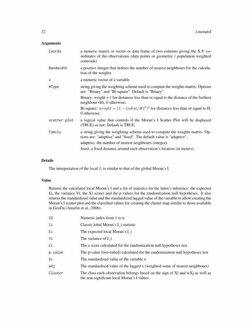
Arguments

Coords a numeric matrix or vector or data frame of two columns giving the X,Y co-ordinates of the observations (data points or geometric / population weightedcentroids)

Bandwidth a positive integer that defines the number of nearest neighbours for the calcula-tion of the weights

x a numeric vector of a variable

WType string giving the weighting scheme used to compute the weights matrix. Optionsare: "Binary" and "Bi-square". Default is "Binary".Binary: weight = 1 for distances less than or equal to the distance of the furthestneighbour (H), 0 otherwise;Bi-square: weight = (1 − (ndist/H)2)2 for distances less than or equal to H,0 otherwise.

scatter.plot a logical value that controls if the Moran’s I Scatter Plot will be displayed(TRUE) or not. Default is TRUE.

family a string giving the weighting scheme used to compute the weights matrix. Op-tions are: "adaptive" and "fixed". The default value is "adaptive".adaptive: the number of nearest neighbours (integer).fixed: a fixed distance around each observation’s location (in meters).

Details

The interpretation of the local Ii is similar to that of the global Moran’s I.

Value

Returns the calculated local Moran’s I and a list of statistics for the latter’s inference: the expectedEi, the variance Vi, the Xi scores and the p-values for the randomization null hypotheses. It alsoreturns the standardized value and the standardized lagged value of the variable to allow creating theMoran’s I scatter plot and the classified values for creating the cluster map similar to those availablein GeoDa (Anselin et al., 2006).

ID Numeric index from 1 to n

Ii Classic lobal Moran’s I_i statistic

Ei The expected local Moran’s I_i

Vi The variance of I_i

Zi The z score calculated for the randomization null hypotheses test

p.value The p-value (two-tailed) calculated for the randomization null hypotheses test

Xi The standardised value of the variable x

wXj The standardised value of the lagged x (weighted some of nearest neighbours)

Cluster The class each observation belongs based on the sign of Xi and wXj as well asthe non-significant local Moran’s I values

lat2w 33

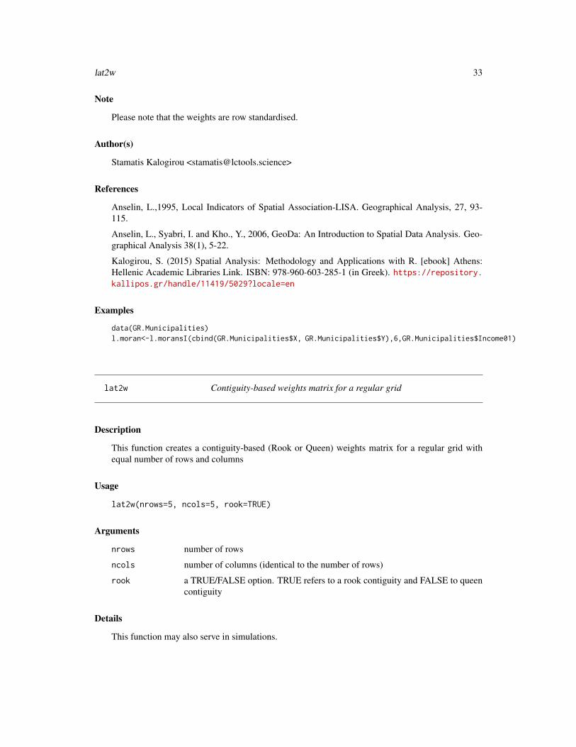
Note

Please note that the weights are row standardised.

Author(s)


References

Anselin, L.,1995, Local Indicators of Spatial Association-LISA. Geographical Analysis, 27, 93-115.

Anselin, L., Syabri, I. and Kho., Y., 2006, GeoDa: An Introduction to Spatial Data Analysis. Geo-graphical Analysis 38(1), 5-22.


Examples

data(GR.Municipalities)l.moran<-l.moransI(cbind(GR.Municipalities$X, GR.Municipalities$Y),6,GR.Municipalities$Income01)

lat2w Contiguity-based weights matrix for a regular grid

Description

This function creates a contiguity-based (Rook or Queen) weights matrix for a regular grid withequal number of rows and columns

Usage

lat2w(nrows=5, ncols=5, rook=TRUE)

Arguments

nrows number of rows

ncols number of columns (identical to the number of rows)

rook a TRUE/FALSE option. TRUE refers to a rook contiguity and FALSE to queencontiguity

Details

This function may also serve in simulations.



34 lcorrel

Value

Returns a list of neighbours for each cell of the grid as well as a weights matrix.

nbs a list of neighbours for each observation

w a matrix of weights

Author(s)


References



See Also

w.matrix, moransI.w, spGini.w

Examples

#rook weights matrix for a 5 by 5 gridw.mat <- lat2w(nrows=5, ncols=5)

lcorrel Local Pearson and GW Pearson Correlation

Description

This function computes Local Pearson and Geographically Weighted Pearson Correlation Coeffi-cients and tests for their statistical significance. Because the local significant tests are not indepen-dent, under the multiple hypotheses testing theory, a Bonferroni correction of the local coefficientstakes place. The function results in tables with results for all possible pairs of the input variables.

Usage

lcorrel(DFrame, bw, Coords)




lcorrel 35

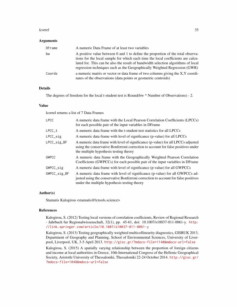
Arguments

DFrame A numeric Data Frame of at least two variablesbw A positive value between 0 and 1 to define the proportion of the total observa-

tions for the local sample for which each time the local coefficients are calcu-lated for. This can be also the result of bandwidth selection algorithms of localregression techniques such as the Geographically Weighted Regression (GWR)

Coords a numeric matrix or vector or data frame of two columns giving the X,Y coordi-nates of the observations (data points or geometric centroids)

Details

The degrees of freedom for the local t-student test is Round(bw * Number of Observations) - 2.

Value

lcorrel returns a list of 7 Data Frames

LPCC A numeric data frame with the Local Pearson Correlation Coefficients (LPCCs)for each possible pair of the input variables in DFrame

LPCC_t A numeric data frame with the t-student test statistics for all LPCCsLPCC_sig A numeric data frame with level of significance (p-value) for all LPCCsLPCC_sig_BF A numeric data frame with level of significance (p-value) for all LPCCs adjusted

using the conservative Bonferroni correction to account for false positives underthe multiple hypothesis testing theory

GWPCC A numeric data frame with the Geographically Weighted Pearson CorrelationCoefficients (GWPCCs) for each possible pair of the input variables in DFrame

GWPCC_sig A numeric data frame with level of significance (p-value) for all GWPCCsGWPCC_sig_BF A numeric data frame with level of significance (p-value) for all GWPCCs ad-

justed using the conservative Bonferroni correction to account for false positivesunder the multiple hypothesis testing theory

Author(s)


References

Kalogirou, S. (2012) Testing local versions of correlation coefficients, Review of Regional Research- Jahrbuch fur Regionalwissenschaft, 32(1), pp. 45-61, doi: 10.1007/s10037-011-0061-y. http://link.springer.com/article/10.1007/s10037-011-0061-y


Kalogirou, S. (2015) A spatially varying relationship between the proportion of foreign citizensand income at local authorities in Greece, 10th International Congress of the Hellenic GeographicalSociety, Aristotle University of Thessaloniki, Thessaloniki 22-24 October 2014. http://gisc.gr/?mdocs-file=1048&mdocs-url=false






36 mc.lcorrel

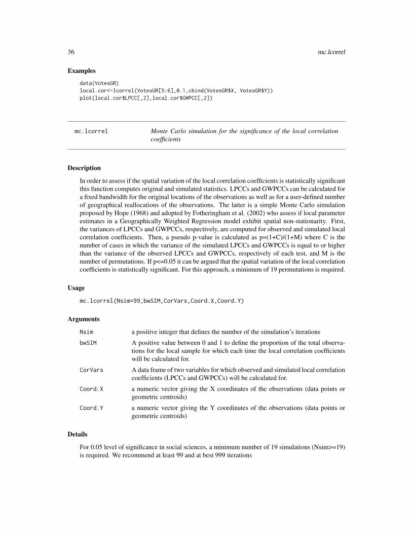
Examples

data(VotesGR)local.cor<-lcorrel(VotesGR[5:6],0.1,cbind(VotesGR$X, VotesGR$Y))plot(local.cor$LPCC[,2],local.cor$GWPCC[,2])

mc.lcorrel Monte Carlo simulation for the significance of the local correlationcoefficients

Description

In order to assess if the spatial variation of the local correlation coefficients is statistically significantthis function computes original and simulated statistics. LPCCs and GWPCCs can be calculated fora fixed bandwidth for the original locations of the observations as well as for a user-defined numberof geographical reallocations of the observations. The latter is a simple Monte Carlo simulationproposed by Hope (1968) and adopted by Fotheringham et al. (2002) who assess if local parameterestimates in a Geographically Weighted Regression model exhibit spatial non-stationarity. First,the variances of LPCCs and GWPCCs, respectively, are computed for observed and simulated localcorrelation coefficients. Then, a pseudo p-value is calculated as p=(1+C)/(1+M) where C is thenumber of cases in which the variance of the simulated LPCCs and GWPCCs is equal to or higherthan the variance of the observed LPCCs and GWPCCs, respectively of each test, and M is thenumber of permutations. If p<=0.05 it can be argued that the spatial variation of the local correlationcoefficients is statistically significant. For this approach, a minimum of 19 permutations is required.

Usage

mc.lcorrel(Nsim=99,bwSIM,CorVars,Coord.X,Coord.Y)

Arguments


bwSIM A positive value between 0 and 1 to define the proportion of the total observa-tions for the local sample for which each time the local correlation coefficientswill be calculated for.

CorVars A data frame of two variables for which observed and simulated local correlationcoefficients (LPCCs and GWPCCs) will be calculated for.

Coord.X a numeric vector giving the X coordinates of the observations (data points orgeometric centroids)

Coord.Y a numeric vector giving the Y coordinates of the observations (data points orgeometric centroids)

Details

For 0.05 level of significance in social sciences, a minimum number of 19 simulations (Nsim>=19)is required. We recommend at least 99 and at best 999 iterations

mc.lcorrel 37

Value

Returns a list of summary statistics for the simulated values of LPCCs and GWPCCs, the observedLPCCs and GWPCCs and the pseudo p-value of significance for the spatial variation of the LPCCsand GWPCCs, respectivelly

SIM a dataframe with simulated values: SIM.ID is the simulation ID, SIM.gwGiniis the simulated Gini of neighbours, SIM.nsGini is the simulated Gini of non-neighbours, SIM.SG is the simulated share of the overall Gini that is associ-ated with non-neighbour pairs of locations, SIM.Extr = 1 if the simulated SG isgreater than or equal to the observed SG

LC.Obs list of 7 Data Frames as in lcorrel

pseudo.p.lpcc pseudo p-value for the significance of the spatial variation of the LPCCs: if thisis lower than or equal to 0.05 it can be argued that the the spatial variation of theLPCCs is statistically significant.

pseudo.p.gwpcc pseudo p-value for the significance of the spatial variation of the GWPCCs: ifthis is lower than or equal to 0.05 it can be argued that the the spatial variationof the GWPCCs is statistically significant.

Author(s)


References

Hope, A.C.A. (1968) A Simplified Monte Carlo Significance Test Procedure, Journal of the RoyalStatistical Society. Series B (Methodological), 30 (3), pp. 582 - 598.

Fotheringham, A.S, Brunsdon, C., Charlton, M. (2002) Geographically Weighted Regression: theanalysis of spatially varying relationships, Chichester: John Wiley and Sons.

Examples

X<-rep(11:14, 4)Y<-rev(rep(1:4, each=4))var1<-c(1,1,1,1,1,1,2,2,2,2,3,3,3,4,4,5)var2<-rev(var1)Nsim= 19bwSIM<-0.5

SIM20<-mc.lcorrel(Nsim,bwSIM, cbind(var1,var2),X,Y)

SIM20$pseudo.p.lpccSIM20$pseudo.p.gwpcc

38 mc.spGini

mc.spGini Monte Carlo simulation for the significance of the Spatial Gini coeffi-cient

Description

This function provides one approach for inference on the spatial Gini inequality measure. This is asmall Monte Carlo simulation according to which: a) the data are spatially reallocated in a randomway; b) the share of overall inequality that is associated with non-neighbour pairs of locations -SG (Eq. 5 in Rey & Smith, 2013) - is calculated for the original and simulated spatial data sets; c)a pseudo p-value is calculated as p=(1+C)/(1+M) where C is the number of the permutation datasets that generated SG values that were as extreme as the observed SG value for the original data(Eq. 6 in Rey & Smith, 2013). If p<=0.05 it can be argued that the component of the Gini for non-neighbour inequality is statistically significant. For this approach, a minimum of 19 simulations isrequired.

Usage

mc.spGini(Nsim=99,Bandwidth,x,Coord.X,Coord.Y,WType='Binary')

Arguments




Coord.X a numeric vector giving the X coordinates of the observations (data points orgeometric centroids)

Coord.Y a numeric vector giving the Y coordinates of the observations (data points orgeometric centroids)

WType string giving the weighting scheme used to compute the weights matrix. Optionsare: "Binary", "Bi-square", "RSBi-square". Default is "Binary".Binary: weight = 1 for distances less than or equal to the distance of the furthestneighbour (H), 0 otherwise;Bi-square: weight = (1-(ndist/H)^2)^2 for distances less than or equal to H, 0otherwise;RSBi-square: weight = Bi-square weights / sum (Bi-square weights) for eachrow in the weights matrix

Details

For 0.05 level of significance in social sciences, a minimum number of 19 simulations (Nsim>=19)is required. We recommend at least 99 and at best 999 iterations

mc.spGini 39

Value

Returns a list of the simulated values, the observed Gini and its spatial decomposition, the pseudop-value of significance

SIM a dataframe with simulated values: SIM.ID is the simulation ID, SIM.gwGiniis the simulated Gini of neighbours, SIM.nsGini is the simulated Gini of non-neighbours, SIM.SG is the simulated share of the overall Gini that is associ-ated with non-neighbour pairs of locations, SIM.Extr = 1 if the simulated SG isgreater than or equal to the observed SG

spGini.Observed

Observed Gini (Gini) and its spatial components (gwGini, nsGini)

pseudo.p pseudo p-value: if this is lower than or equal to 0.05 it can be argued that thecomponent of the Gini for non-neighbour inequality is statistically significant.

Note

Acknowledgement: I would like to thank LI Zai-jun, PhD student at Nanjing Normal University,China for encouraging me to develop this function and for testing this package.

Author(s)


References

Rey, S.J., Smith, R. J. (2013) A spatial decomposition of the Gini coefficient, Letters in Spatial andResource Sciences, 6 (2), pp. 55-70.


Examples

data(GR.Municipalities)Nsim=19Bd1<-4x1<-GR.Municipalities@data$Income01[1:45]WType1<-'Binary'

SIM20<-mc.spGini(Nsim,Bd1,x1,GR.Municipalities@data$X[1:45], GR.Municipalities@data$Y[1:45],WType1)SIM20

hist(SIM20$SIM$SIM.nsGini,col = "lightblue", main = "Observed and simulated nsGini",xlab = "Simulated nsGini", ylab = "Frequency",xlim = c(min(SIM20$SIM$SIM.nsGini),SIM20$spGini.Observed[[3]]))abline(v=SIM20$spGini.Observed[[3]], col = 'red')



40 moransI

moransI Moran’s I classic statistic for assessing spatial autocorrelation

Description

Moran’s I is one of the oldest statistics used to examine spatial autocorrelation. This global statisticwas first proposed by Moran (1948, 1950). Later, Cliff and Ord (1973, 1981) present a comprehen-sive work on spatial autocorrelation and suggested a formula to calculate the I which is now used inmost textbooks and software:

I = (n/W ) ∗ (ΣΣwij ∗ zi ∗ zj/Σz2i )

where n is number of observations, W is the sum of the weights w_ij for all pairs in the system,zi = xi −mean(x) where x is the value of the variable at location i and mean(x) the mean valueof the variable in question (Eq. 5.2 Kalogirou, 2003).The implementation here allows only nearestneighbour weighting schemes. Resampling and randomization null hypotheses have been testedfollowing the discussion of Goodchild (1986, pp. 24-26).

Usage

moransI(Coords, Bandwidth, x, WType = 'Binary')

Arguments




WType a string giving the weighting scheme used to compute the weights matrix. Op-tions are: "Binary" and "Bi-square". Default is "Binary".Binary: weight = 1 for distances less than or equal to the distance of the furthestneighbour (H), 0 otherwise;Bi-square: weight = (1 − (ndist/H)2)2 for distances less than or equal to H,0 otherwise.

Details

The Moran’s I statistic ranges from -1 to 1. Values in the interval (-1, 0) indicate negative spatialautocorrelation (low values tend to have neighbours with high values and vice versa), values near0 indicate no spatial autocorrelation (no spatial pattern - random spatial distribution) and values inthe interval (0,1) indicate positive spatial autocorrelation (spatial clusters of similarly low or highvalues between neighbour municipalities should be expected.)

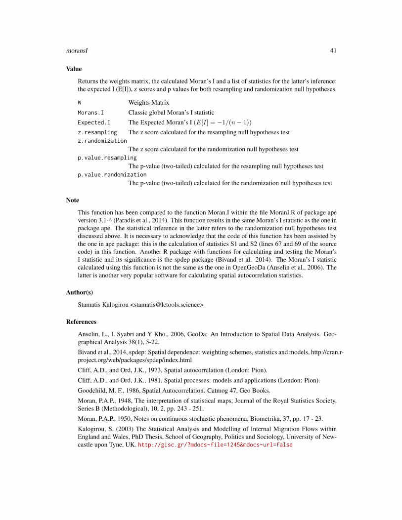
moransI 41

Value

Returns the weights matrix, the calculated Moran’s I and a list of statistics for the latter’s inference:the expected I (E[I]), z scores and p values for both resampling and randomization null hypotheses.

W Weights Matrix

Morans.I Classic global Moran’s I statistic

Expected.I The Expected Moran’s I (E[I] = −1/(n− 1))

z.resampling The z score calculated for the resampling null hypotheses testz.randomization

The z score calculated for the randomization null hypotheses testp.value.resampling

The p-value (two-tailed) calculated for the resampling null hypotheses testp.value.randomization

The p-value (two-tailed) calculated for the randomization null hypotheses test

Note

This function has been compared to the function Moran.I within the file MoranI.R of package apeversion 3.1-4 (Paradis et al., 2014). This function results in the same Moran’s I statistic as the one inpackage ape. The statistical inference in the latter refers to the randomization null hypotheses testdiscussed above. It is necessary to acknowledge that the code of this function has been assisted bythe one in ape package: this is the calculation of statistics S1 and S2 (lines 67 and 69 of the sourcecode) in this function. Another R package with functions for calculating and testing the Moran’sI statistic and its significance is the spdep package (Bivand et al. 2014). The Moran’s I statisticcalculated using this function is not the same as the one in OpenGeoDa (Anselin et al., 2006). Thelatter is another very popular software for calculating spatial autocorrelation statistics.

Author(s)


References

Anselin, L., I. Syabri and Y Kho., 2006, GeoDa: An Introduction to Spatial Data Analysis. Geo-graphical Analysis 38(1), 5-22.

Bivand et al., 2014, spdep: Spatial dependence: weighting schemes, statistics and models, http://cran.r-project.org/web/packages/spdep/index.html

Cliff, A.D., and Ord, J.K., 1973, Spatial autocorrelation (London: Pion).

Cliff, A.D., and Ord, J.K., 1981, Spatial processes: models and applications (London: Pion).

Goodchild, M. F., 1986, Spatial Autocorrelation. Catmog 47, Geo Books.

Moran, P.A.P., 1948, The interpretation of statistical maps, Journal of the Royal Statistics Society,Series B (Methodological), 10, 2, pp. 243 - 251.

Moran, P.A.P., 1950, Notes on continuous stochastic phenomena, Biometrika, 37, pp. 17 - 23.



42 moransI.v


Paradis et al., 2014, ape: Analyses of Phylogenetics and Evolution, http://ape-package.ird.fr/

Examples

data(GR.Municipalities)attr<[email protected]<-moransI(cbind(attr$X, attr$Y),6,attr$UnemrT01)

t(as.matrix(m.I[2:7]))

moransI.v Computes a vector of Moran’s I statistics.

Description



where n is number of observations, W is the sum of the weights w_ij for all pairs in the system,zi = xi −mean(x) where x is the value of the variable at location i and mean(x) the mean valueof the variable in question (Eq. 5.2 Kalogirou, 2003).

This function allows the computation of an number of Moran’s I statistics of the same family (fixedor adaptive) with different kernel size. To achieve this it first computes the weights matrix using thew.matrix function and then computes the Moran’s I using the moransI.w function for each kernel.The function returns a table with the results and a simple scatter plot with the Moran’s I and thekernel size. The latter can be disabled by the user.

Usage

moransI.v(Coords, Bandwidths, x, WType='Binary', family='adaptive', plot = TRUE)

Arguments


Bandwidths a vector of positive integers that defines the number of nearest neighbours for thecalculation of the weights or a vector of Bandwidths relevant to the coordinatesystems the spatial analysis refers to.



http://ape-package.ird.fr/


moransI.v 43


WType a string giving the weighting function used to compute the weights matrix. Op-tions are: "Binary", "Bi-square", and "RSBi-square". The default value is "Bi-nary".Binary: weight = 1 for distances less than or equal to the distance of the furthestneighbour (H), 0 otherwise;Bi-square: weight = (1-(ndist/H)^2)^2 for distances less than or equal to H, 0otherwise;RSBi-square: weight = Bi-square weights / sum (Bi-square weights) for eachrow in the weights matrix


plot a logical value (TRUE/FALSE) denoting whether a scatter plot with the Moran’sI and the kernel size will be created (if TRUE) or not.

Details


Value

Returns a matrix with 8 columns and plots a scatter plot. These columns present the followingstatistics for each kernel size:

ID an integer in the sequence 1:m, where m is the number of kernel sizes in thevector Bandwidths

k the kernel size (number of neighbours or distance)

Moran’s I Classic global Moran’s I statistic

Expected I The Expected Moran’s I (E[I]=-1/(n-1))

Z resampling The z score calculated for the resampling null hypotheses testP-value resampling

The p-value (two-tailed) calculated for the resampling null hypotheses testZ randomization

The z score calculated for the randomization null hypotheses testP-value randomization


Author(s)


44 moransI.w

References








See Also

moransI.w, w.matrix

Examples

data(GR.Municipalities)Coords<-cbind(GR.Municipalities@data$X, GR.Municipalities@data$Y)

#using an adaptive kernelbws <- c(3, 4, 6, 9, 12, 18, 24)moransI.v(Coords, bws, GR.Municipalities@data$Income01)

moransI.w Moran’s I classic statistic for assessing spatial autocorrelation usinga ready made weights matrix.

Description



where n is number of observations, W is the sum of the weights w_ij for all pairs in the system,zi = xi −mean(x) where x is the value of the variable at location i and mean(x) the mean valueof the variable in question (Eq. 5.2 Kalogirou, 2003).

The implementation here allows for the use of a weights matrix that could use any weighting schemecreated either within lctools (using the w.matrix function) or other R packages. Resampling andrandomization null hypotheses have been tested following the discussion of Goodchild (1986, pp.24-26).




moransI.w 45

Usage

moransI.w(x, w)

Arguments


w Weights Matrix usin w.matrix or other R function

Details


Value

Returns the calculated Moran’s I and a list of statistics for the latter’s inference: the expected I(E[I]), z scores and p values for both resampling and randomization null hypotheses.

Morans.I Classic global Moran’s I statistic

Expected.I The Expected Moran’s I (E[I]=-1/(n-1))

z.resampling The z score calculated for the resampling null hypotheses testz.randomization

The z score calculated for the randomization null hypotheses testp.value.resampling

The p-value (two-tailed) calculated for the resampling null hypotheses testp.value.randomization


Note

I would like to acknowledge the use of some lines of code from the file MoranI.R of the packageape and I would like to thank Paradis et al. (2016) and all authors involved in the Moran’s I functionfor this.

Author(s)


References

Anselin, L., I. Syabri and Y Kho., 2006, GeoDa: An Introduction to Spatial Data Analysis. Geo-graphical Analysis 38(1), 5-22.

Bivand et al., 2014, spdep: Spatial dependence: weighting schemes, statistics and models, http://cran.r-project.org/web/packages/spdep/index.html

46 random.test.data








Paradis et al., 2016, ape: Analyses of Phylogenetics and Evolution, http://ape-package.ird.fr/

See Also

moransI, w.matrix

Examples

data(GR.Municipalities)attr <- GR.Municipalities@data

#using an adaptive kernelw.ad <- w.matrix(cbind(attr$X, attr$Y),6)mI.ad <- moransI.w(attr$UnemrT01,w.ad)as.data.frame(mI.ad)

#using a fixed kernelw.fixed<-w.matrix(cbind(attr$X, attr$Y), 50000, WType='Binary', family='fixed')mI.fixed<-moransI.w(attr$UnemrT01,w.fixed)as.data.frame(mI.fixed)

random.test.data Radmom data generator

Description

Generates datasets with random data for modelling including a dependent variable, independentvariables and X,Y coordinates.

Usage

random.test.data(nrows = 10, ncols = 10, vars.no = 3, dep.var.dis = "normal",xycoords = TRUE)






spg.sim.test 47

Arguments

nrows an integer referring to the number of rows for a regular grid

ncols an integer referring to the number of columns for a regular grid

vars.no an integer referring to the number of independent variables

dep.var.dis a character referring to the distribution of the dependent variable. Options are"normal" (default), "poisson", and "zip"

xycoords a logical value indicating whether X,Y coordinates will be created (default) ornot.

Details

The creation of a random dataset was necessary here to provide examples to some functions. How-ever, random datasets may be used in simulation studies.

Value

a dataframe

Author(s)


Examples

RDF <- random.test.data(12,12,3,"poisson")

spg.sim.test Simulation test (Rey & Smith, 2013))

Description

This is a simulation test presented by Rey & Smith (2013) as part of the inference for the spatialdecomposition of the Gini coefficient.

Usage

spg.sim.test(realizations = 1000, nperm = 99)

Arguments

realizations Number of realizations of the simulation.

nperm Number of permutations of simulated spatial autocorrelation and spatial ginisimulations for each realization.

48 spg.sim.test

Details

This function implements the simulation presented in pages 63-66 of the paper by Rey & Smith(2013). The results of this function should be comparable to the Figures 1, 2 and 3. However, thecurrent implementation of this function results in different frequencies.

Value

A list of results:

res

moran_res

gini_mean

gini_std

moran_mean

Warning

This simulation takes time to complete and the results may not match those presented in the paperby Rey and Smith (2013).

Note

This function is under development.

Author(s)


References


See Also

mc.spGini spGini

spGini 49

spGini Spatial Gini coefficient

Description

This is the implementation of the spatial decomposition of the Gini coefficient introduced by Reyand Smith (2013). The function calculates the global Gini and the two components of the spa-tial Gini: the inequality among nearest (geographically) neighbours and the inequality of non-neighbours. Three weighted schemes are currently supported: binary, bi-square and row standard-ised bi-square.

Usage

spGini(Coords, Bandwidth, x, WType = 'Binary')

Arguments



x a numeric vector of a variableWType a string giving the weighting scheme used to compute the weights matrix. Op-

tions are: "Binary", "Bi-square", "RSBi-square". Default is "Binary".Binary: weight = 1 for distances less than or equal to the distance of the furthestneighbour (H), 0 otherwise;Bi-square: weight = (1-(ndist/H)^2)^2 for distances less than or equal to H, 0otherwise;RSBi-square: weight = Bi-square weights / sum (Bi-square weights) for eachrow in the weights matrix

Value

Returns a list of five values Gini, gwGini, nsGini, gwGini.frac, nsGini.frac

Gini Global GinigwGini First component of the spatial Gini: the inequality among nearest (geographi-

cally) neighboursnsGini Second component of the spatial Gini: the inequality among non-neighboursgwGini.frac The fraction of the first component of the spatial GininsGini.frac The fraction of the second component of the spatial Gini

Author(s)


50 spGini.w

References



Examples

data(GR.Municipalities)Coords1<-cbind(GR.Municipalities@data$X, GR.Municipalities@data$Y)Bandwidth1<-12x1<-GR.Municipalities@data$Income01WType1<-'Binary'spGini(Coords1,Bandwidth1,x1,WType1)

spGini.w Spatial Gini coefficient with a given weights matrix

Description

This is the implementation of the spatial decomposition of the Gini coefficient introduced by Reyand Smith (2013) as in the function spGini. In this function, the calculation of the global Gini andthe two components of the spatial Gini is performed using matrix algebra and a ready made weightsmatrix. Thus, it is possible to use weighting schemes other than those currently supported in spGini.

Usage

spGini.w(x, w)

Arguments


w Weights Matrix usin w.matrix or other R function

Value

Returns a list of five values Gini, gwGini, nsGini, gwGini.frac, nsGini.frac

Gini Global Gini

gwGini First component of the spatial Gini: the inequality among nearest (geographi-cally) neighbours

nsGini Second component of the spatial Gini: the inequality among non-neighbours

gwGini.frac The fraction of the first component of the spatial Gini

nsGini.frac The fraction of the second component of the spatial Gini



VotesGR 51

Author(s)


References



Examples

data(GR.Municipalities)w<-w.matrix(cbind(GR.Municipalities@data$X, GR.Municipalities@data$Y),12,WType='Binary')spGini.w(GR.Municipalities@data$Income01,w)

VotesGR New Democracy and Total Votes in Greece in 2012

Description

New Democracy and Total Votes per prefecture in the double parliamentary elections in Greece inMay and June 2012, respectively

Usage

data(VotesGR)

Format

A data frame with 51 observations on the following 8 variables.

MapCode2 a numeric vector of codes for joining this data to a mapNAME_ENG a alphanumeric vector of prefecture names in greeklishX a numeric vector of x coordinatesY a numeric vector of y coordinatesNDJune12 a numeric vector of votes for New Democracy in June 2012 parliamentary electionsNDMay12 a numeric vector of votes for New Democracy in May 2012 parliamentary electionsAllJune12 a numeric vector of total valid votes in June 2012 parliamentary electionsAllMay12 a numeric vector of total valid votes in May 2012 parliamentary elections

Details

The X,Y coordinates refer to the geometric centroids of the 51 Prefectures in Greece in 2011. Allelectoral districts in the Attica Region have been merged to one. The two electoral regions inThessaloniki have also been merged to a single region matching the NUTS II regions geography.



52 w.matrix

Source

The shapefile of the corresponding polygons is available from the Public Open Data of the GreekGovernment at http://geodata.gov.gr/en/dataset/oria-nomon-okkhe. The election results(votes) are available from the Hellenic Ministry of Interior at http://www.ypes.gr/en/Elections/NationalElections/Results/.

References

Georganos, S., Kalogirou, S. (2014) Spatial analysis of voting patterns of national elections inGreece, 10th International Congress of the Hellenic Geographical Society, Aristotle University ofThessaloniki, Thessaloniki 22-24 October 2014.

Examples

data(VotesGR)plot(VotesGR$NDJune12,VotesGR$NDMay12)abline(0,1)

w.matrix Weights Matrix based on a number of nearest neighbours or a fixeddistance

Description

This function constructs an n by n weights matrix for a geography with n geographical elements(e.g. points or polygons) using a number of nearest neighbours or a fixed distance.

Usage

w.matrix(Coords, Bandwidth, WType = "Binary", family = "adaptive")

Arguments

Coords a numeric matrix or vector or data frame of two columns giving the X,Y co-ordinates of the geographical elements (data points or geometric / populationweighted centroids for polygons)

Bandwidth either a positive integer that defines the number of nearest neighbours for thecalculation of the weights of an adaptive kernel (family = ’adaptive’) or a fixeddistance in meters for a fixed kernel (family = ’fixed’).

WType a string giving the weighting function used to compute the weights matrix. Op-tions are: "Binary", "Bi-square", and "RSBi-square". The default value is "Bi-nary".Binary: weight = 1 for distances less than or equal to the distance of the furthestneighbour (H), 0 otherwise;Bi-square: weight = (1-(ndist/H)^2)^2 for distances less than or equal to H, 0otherwise;RSBi-square: weight = Bi-square weights / sum (Bi-square weights) for eachrow in the weights matrix

http://geodata.gov.gr/en/dataset/oria-nomon-okkhe

http://www.ypes.gr/en/Elections/NationalElections/Results/

http://www.ypes.gr/en/Elections/NationalElections/Results/

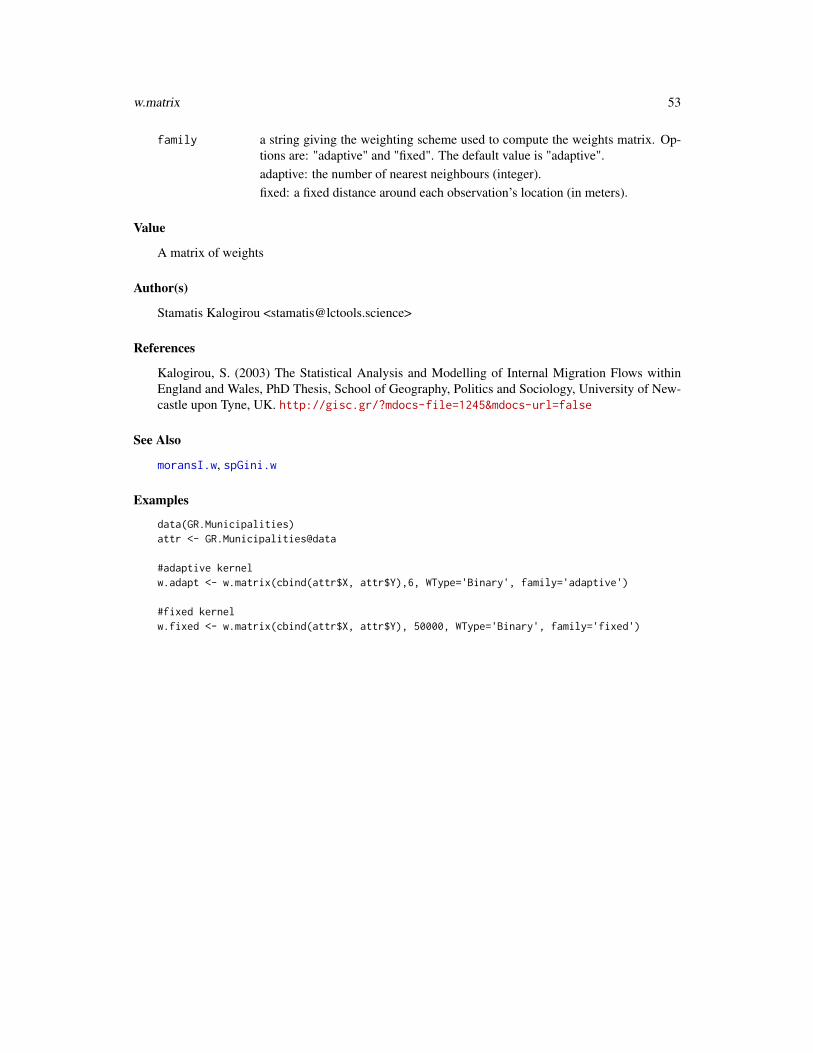
w.matrix 53


Value

A matrix of weights

Author(s)


References


See Also

moransI.w, spGini.w

Examples

data(GR.Municipalities)attr <- GR.Municipalities@data

#adaptive kernelw.adapt <- w.matrix(cbind(attr$X, attr$Y),6, WType='Binary', family='adaptive')

#fixed kernelw.fixed <- w.matrix(cbind(attr$X, attr$Y), 50000, WType='Binary', family='fixed')


Index

∗Topic Competing Destinations Modelacc, 4

∗Topic FLQFLQ, 5

∗Topic Focal Location QuotientFLQ, 5

∗Topic GGWRgw.glm.light, 13gw.glm.mc.test, 14

∗Topic GWPCCs inferencemc.lcorrel, 36

∗Topic GWPCClcorrel, 34

∗Topic GWPRgw.glm, 8gw.glm.cv, 12

∗Topic GWRgw.glm.bw, 10gw.zi.bw, 18gwr, 25gwr.bw, 27gwr.cv, 29lctools-package, 2

∗Topic GWZIPRgw.zi, 16gw.zi.cv, 20gw.zi.light, 21gw.zi.mc.test, 23

∗Topic GinispGini, 49spGini.w, 50

∗Topic Greek MunicipalitiesGR.Municipalities, 6

∗Topic Inferencegw.glm.mc.test, 14gw.zi.mc.test, 23mc.spGini, 38

∗Topic LISAl.moransI, 31

∗Topic LPCCs inferencemc.lcorrel, 36

∗Topic LPCClcorrel, 34

∗Topic LQFLQ, 5

∗Topic Location QuotientFLQ, 5

∗Topic Monte Carlo Simulationgw.glm.mc.test, 14gw.zi.mc.test, 23mc.lcorrel, 36mc.spGini, 38

∗Topic Moran’s I Clustersl.moransI, 31

∗Topic Moran’s I significance testmoransI, 40moransI.v, 42moransI.w, 44

∗Topic Moran’s ImoransI, 40moransI.v, 42moransI.w, 44

∗Topic Regular Grid Weights Matrixlat2w, 33

∗Topic Simulationspg.sim.test, 47

∗Topic Spatial Analysislat2w, 33w.matrix, 52

∗Topic Spatial Ginimc.spGini, 38spg.sim.test, 47spGini, 49spGini.w, 50

∗Topic Spatial Inequalitymc.spGini, 38spg.sim.test, 47spGini, 49

54

INDEX 55

spGini.w, 50∗Topic Spatial autocorrelation

mc.spGini, 38moransI, 40moransI.v, 42moransI.w, 44spg.sim.test, 47spGini, 49spGini.w, 50

∗Topic Weights Matrixw.matrix, 52

∗Topic accessibilityacc, 4

∗Topic centralityacc, 4

∗Topic datasetsGR.Municipalities, 6VotesGR, 51

∗Topic geographical boundariesGR.Municipalities, 6

∗Topic geographically weightedvariable

gw_variable, 30∗Topic geostatistics

lctools-package, 2∗Topic local Moran’s I

l.moransI, 31∗Topic local multi-collinearity

lcorrel, 34mc.lcorrel, 36

∗Topic local regressiongw.glm, 8gw.glm.cv, 12gw.glm.light, 13gw.glm.mc.test, 14gw.zi, 16gw.zi.cv, 20gw.zi.light, 21gw.zi.mc.test, 23gwr, 25gwr.cv, 29

∗Topic optimal bandwidthgw.glm.bw, 10gw.zi.bw, 18gwr.bw, 27

∗Topic packagelctools-package, 2

∗Topic random data

random.test.data, 46∗Topic regional variable

gw_variable, 30∗Topic spatial analysis

lctools-package, 2∗Topic spatial inequalities

lctools-package, 2

acc, 4

FLQ, 5formula, 8, 10, 12, 13, 15, 25, 27, 29

glm, 8–10, 12, 13, 15GR.Municipalities, 6gw.glm, 8, 12–14, 16, 18, 24, 26gw.glm.bw, 9, 10, 13, 16gw.glm.cv, 12, 12gw.glm.light, 13, 14gw.glm.mc.test, 14, 14gw.zi, 9, 16, 20–23, 26gw.zi.bw, 18, 18, 21, 24gw.zi.cv, 20, 20gw.zi.light, 21, 22gw.zi.mc.test, 22, 23, 23gw_variable, 30gwr, 9, 11, 16, 18, 20, 24, 25, 28–30gwr.bw, 26, 27, 30gwr.cv, 29, 29

l.moransI, 31lat2w, 33lcorrel, 34lctools (lctools-package), 2lctools-package, 2lm, 25, 27, 29

mc.lcorrel, 36mc.spGini, 38, 48moransI, 40, 46moransI.v, 42moransI.w, 34, 44, 44, 53

optim, 10, 11, 19, 27, 28

random.test.data, 46

spg.sim.test, 47spGini, 48, 49spGini.w, 34, 50, 53

56 INDEX

VotesGR, 51

w.matrix, 34, 44, 46, 52

zeroinfl, 16, 18, 20, 22, 23

package ‘lctools’ - r · package ‘lctools ’ april 23, 2019 ... gression methods including...

Documents